


Introduction
The extent and nature of the polar ice sheets are of interest to workers in a variety of fields, particularly climatology and navigation. Passive microwave radiation observations of the Arctic and Antarctic have been used successfully in mapping the spatial and temporal evolution of the ice water boundary and the percentage of old ice as opposed to new ice (Reference Campbell, Campbell, Gloersen, Nordberg, Wilheit, Bock and BockCampbell and others, 1974, Reference Campbell, Campbell, Weeks, Ramseier and Gloersen1975; Reference Gloersen, Gloersen, Zwally, Chang, Hall, Campbell and RamseierGloersen and others, 1978). Differences in the microwave signatures between old ice, new ice, and water have also been observed (Reference Wilheit, Wilheit, Nordberg, Blinn, Campbell and EdgertonWilheit and others, 1972; Reference Gloersen, Gloersen, Nordberg, Schmugge, Wilheit and CampbellGloersen and others, 1973; Reference Tooma, Tooma, Mennella, Hollinger and KetchumTooma and others, 1975). Moreover, the long-term snow-accumulation rates for Greenland and Antarctica have been estimated from microwave signatures (Reference ZwallyZwally, 1977; Reference Rotman, Rotman, Fisher and StaelinRotman and others, in press).
Cluster-analysis techniques were applied to satellite observations of brightness temperature at two frequencies v (22.235 and 31.65 GHz) and seven angles θ over the polar regions, (lat. 70–80°, north and south); thus 14-dimensional feature vectors were formed. Unsupervised “hierarchical” techniques were employed (making no a priori assumptions about the possible classes) in order to study the basic information content of these data (Reference NagyNagy, 1968). Well-defined clusters were produced which tended to include data from points in geographical proximity. In fact, the clustering process effectively performed automatic pattern recognition for a variety of snow and ice classes. Additionally, the average of all the data in each class at a given angle θ and frequency v provided typical brightness-temperature “signatures” T b(θ, v) for the various snow and ice types (Reference Fisher, Fisher, Rotman and StaelinFisher and others, [1978]). The angular data have proven efficient in distinguishing mixtures of new ice with water from uniform old ice. This longstanding problem is encountered when observations at only a single angle are employed, because the brightness temperature for some mixtures of new ice and water can be identical with that for old ice (Reference Gloersen, Gloersen, Wilheit, Chang, Nordberg and CampbellGloersen and others, 1974; Reference Webster, Webster, Wilheit, Chang, Gloersen and SchmuggeWebster and others, 1975).
Satellite and ground-truth data
The Scanning Microwave Spectrometer (SCAMS) on board the Nimbus-6 satellite observed the Earth’s surface at 22.235 and 31.65 GHz from July 1975 to May 1976. At these frequencies, the Earth’s surface was mapped with spatial resolutions of 145 km near nadir and 330 km at the scan limit; the seven angles θ from the satellite relative to nadir were: 0.0°, 7.2°, 14.4°, 21.6°, 28.8°, 36.0°, and 43.2° (Reference Staelin, Staelin, Rosenkranz, Barath, Johnston and WatersStaelin and others, 1977). Because SCAMS incorporated a rotating mirror, the polarization vector rotated with scan angle θ such that the observed brightness temperature T b was T h cos2 θ + T v sin2 θ, where T h and T v were the brightness temperatures due to the horizontally and vertically polarized radiation components respectively. Due to the Earth’s curvature, the zenith angles of observation ϕ at the terrestrial surface were 0.0°, 8.4°, 16.9°, 25.6°, 34.4°, 43.5°, and 53.3°.
Fourteen-dimensional “feature vectors” (brightness temperatures from seven angles at two frequencies) were generated from the satellite observations for 900 locations in the Arctic and 900 in the Antarctic at each of three periods (approximately one-week intervals in September, November, and January). After vectors with missing components were excluded, approximately seven hundred valid vectors remained from each of the original data sets.
The results of our analysis of the microwave data were compared with the actual known surface conditions. Knowledge of this ground truth was available from two sources. First, long-term data were available for the accumulation rate of snow in Antarctica and Greenland (Reference FristrupFristrup, 1966, p. 234; Bentley and others, 1964) and for the extent of the permanent ice pack (Reference Brush and BrushBrush and others, 1966, p. 180). Second, seasonal data for the partial ice cover in the Arctic and Antarctic have been obtained for specific years (U.S. Navy Dept. Fleet Weather Facility, [1976[a], [b]], [1977]) based on the ESMR radiometers on the Nimbus-5 and Nimbus-6 satellites (Reference Gloersen, Gloersen, Wilheit, Chang, Nordberg and CampbellGloersen and others, 1974) and on ground observations.
Clustering theory
The overall objective of cluster analysis is to lump “similar” feature vectors into a common class, while dissimilar feature vectors are placed in distinct classes (Reference NagyNagy, 1968).
An agglomerative hierarchical approach was employed in which the clustering process was initiated by treating each vector as a one-member cluster. The Euclidian distance between each possible pair of vectors in the data set was computed and stored as a “similarity” measure. Then the similarity threshold for which two clusters are combined was increased monotonically to form new clusters, until all the vectors in the data set were combined into one cluster. All the clusters at a given intermediate threshold could be reproduced later. Many options exist for computing the distances between newly formed clusters; the techniques used were single-link and complete-link clustering. In the complete-link approach, the similarity between any two clusters is taken as the furthest Euclidian distance between the elements (14-dimensional vectors) in each cluster; in single-link clustering, the least distance is used (Reference AnderbergAnderberg, 1973).
Once the clusters were formed, two processing methods were used. First, contours of clusters at various distance thresholds were replotted into the geographic maps of Antarctica and Greenland. Second, signatures were created for each cluster by plotting the mean values of the brightness temperatures as a function of angle for both 31 and 22 GHz.
These unsupervised clustering techniques have the advantage of providing an “objective” indication of the information embedded in the basic variation of brightness temperature with angle and frequency. No theoretical model or a priori information is employed. There is a danger that the primary data T b(θ, v) represent such a complex mixture of meaningful parameters that mere position in 14-dimensional feature space will have no bearing on the kinds of information desired. However, a variety of techniques can be employed to evaluate the clusters. In particular, geographically connected areas should tend to be grouped in the same class since neighboring areas will often have the same physical characteristics; the clusters should indicate physically meaningful geographic areas. For example, clusters should follow contours of constant accumulation and temperature—or combinations thereof—of the ice-water boundary.
Moreover, reduction of the size of our vector space is possible by using the Karhunen- Loève method (Reference Duda and HartDuda and Hart, 1973). In this analysis, the correlation matrix is computed, and the coordinate system is then rotated to point along orthogonal trends in the data set. Preliminary studies show that our 14-dimensional data set can be reduced to seven dimensions in this newly rotated coordinate system without losing significant information (Reference Fisher, Fisher, Rotman and StaelinFisher and others, [1978]); these seven orthogonal vectors have no simple relationship to identifiable physical parameters.

Fig. 1. Map of the Antarctic region for September 1975 with six clusters (elliptical projection). The symbols for different clusters are arbitrary.
Experimental results
Excellent results were obtained for the clustering of the brightness-temperature data. Distinct geographical clusters appeared for both the Arctic and Antarctic regions for all three seasons with both complete- and single-link clustering. The maps presented in this paper were produced by complete-link clustering.
Figure 1 shows Antarctica in September 1975 (winter in this area) with six clusters within the latitudes of 70° to 80° S. The band structure of the clusters in Eastern Antarctica is closely related to the accumulation rate and temperature contours (which to some extent are correlated with each other) as determined by surface information and other satellite observations (Reference Rotman, Rotman, Fisher and StaelinRotman and others, in press; Reference Bentley, Bentley, Cameron, Bull, Kojima and GowBentley and others, 1964). A cluster which seems to represent the lowest accumulation-rate areas, formed in the regions (1) lat. 76° to 79° S., long. 30° E., and (2) lat. 76° to 79° S., long. 140° E. (symbol “o”). Clusters “o”, “1”, “2”, “3”, and “4” represent the areas of firn in Eastern Antarctica in order of increasing accumulation rate and temperature as determined from ground data (Reference Bentley, Bentley, Cameron, Bull, Kojima and GowBentley and others, 1964), Cluster “4” is also firn in Western Antarctica with a slight overlap onto sea ice. The area of low accumulation rate at approximately 120° W., 78-79° S., stands out clearly. Sea ice is shown by cluster “5”.
In Figure 2, the data from the Arctic region are grouped into 14 clusters for November 1975. The clustering contours in Greenland (clusters “0”-“5”) seem to follow accumulation contours rather than temperature contours (Reference FristrupFristrup, 1966. p. 230; Gloersen and others, 1974 Reference Zwally; Zwally, 1977). Clusters “6”, “9”, and “10” are representative of the permanent ice pack; its outline is indicated in Figure 2 by the broken line, as determined from ground-truth observations (Reference Brush and BrushBrush and others, 1966, p. 180). Old sea ice is also found cast of Greenland, as shown by the presence of data points grouped into clusters “6” and “9”. The open expanses of water are indicated by the low brightness temperature of cluster “13”; bare ground in Siberia is contained in cluster “12”.

Fig. 2. Map of the Arctic region for November 1975 with fourteen clusters.
The mean values of the brightness temperatures for each cluster were plotted as a function of angle. Typical signatures can be seen in Figures 3, 4, 5, and 6. Observations of the surface show the following general order of increasing brightness temperatures: (1) water, (2) firn (brightness temperature increasing with accumulation), (3) multi-year sea ice (brightness temperature decreasing with age), (4) first-year ice, and (5) bare ground. The shapes of the curves are very informative although separate polarization information is lacking. Additional study of these signatures should clarify the degree to which the volume-scattering in the medium arises from spherical or layered inhomogeneities (Reference Tsang and KongTsang and Kong, 1975, Reference Tsang and Kong1976; Reference Chang, Chang, Gloersen, Schmugge, Wilheit and ZwallyChang and others, 1976; Reference FisherFisher, 1977).

Fig. 3. Typical microwave signatures of Antarctic firn for September 1975 (clusters “0”, “1”, and “3” from Figure 1 for low, medium, and high accumulation rates, respectively)


Fig. 5. Typical microwave signatures of Arctic multi-year sea ice and water for September 1975 (clusters “10” and “13” from Figure 2 for multi-year sea ice and water, respectively)

Fig. 6. Typical microwave signature of Arctic bare ground for September 1975 (cluster “12” from Figure 2).
Applications
Microwave signatures can differentiate between new sea ice mixed with water and old sea ice. This distinction is difficult to obtain from nadir data alone. Since the brightness temperature of new sea ice is very high (240 K) and that from water relatively low (160 K), an equal mixture of the two will be approximately 200 K, which is the same temperature as old sea ice. However, the angular data will differ for the two surfaces since the brightness temperature of a mixture of new sea ice and water shows an increase with angle from nadir, corresponding to the behavior for sea-water alone (Reference Edgerton, Edgerton, Ruskey, Williams, Stogryn, Poe, Meeks and RussellEdgerton and others, 1971), while that of multi-year sea ice decreases.
A simple algorithm was developed to classify SCAMS observations as originating from either old ice or a mixture of new ice and water. Each experimental vector was compared to theoretical signatures for a mixture of new ice and water and assigned to that percentage of new ice with which it best agreed in a least-squares sense. Then the experimental signatures were tested to determine whether they represent old ice or a mixture of new ice and water. Their angular variations were compared to the angular variations of the signature which was obtained previously for the ice-water mixture and to those of the signature for old ice. In this last comparison, the average brightness temperature over all angles was eliminated from the signatures. This reduced the effects of variations of physical temperatures.
Figure 7 shows these results for the North Pole in September; they agree well with the permanent ice pack which is known to exist between long. 120° E. and 120° W. and at long. 20° W. (Reference Campbell, Campbell, Weeks, Ramseier and GloersenCampbell and others, 1975; Reference Brush and BrushBrush and others, 1966, p. 180). Mixtures of ice and water appear to the east of Greenland while wide expanses of water appear between long. 0° and 90° W. and at long. 60° E.
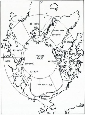
Fig. 7. The partial ice cover of the Arctic region derived from microwave data between lat. 70°-80° N. for September 1975. Percentages shown are the amounts of open water compared to sea ice within each resolution cell of the radiometer (150 km by 150 km) in increments of 10%. The dashed line is the multi-year sea-ice limit (Reference Brush and BrushBrush and others, 1966, p. 180).
Figure 8 shows the seasonal changes from Figure 7 for the North Pole region in January. As we would expect, the area of permanent ice pack has not grown over the winter. However, new sea ice now replaces the open water or partial ice cover seen in September at long. 70° W. and 60° to 120° E. The partial ice cover located east of Greenland has expanded; open water still remains north of Norway. These seasonal observations agree well with ground observations (U.S. Navy Dept. Fleet Weather Facility, [1976[a], [b]], [1977]). It is interesting to note that most of the non-permanent ice-pack area is either c. 100% new ice or c. 100% water; mixtures comprise only c. 10% of the observed area.

Fig. 8. The partial ice cover of the Arctic region derived from SCAMS data between lat. 70°-80° N. for January 1976.
Moreover, the age of the permanent ice pack can be determined by its brightness temperature. As the ice ages, the brightness temperature decreases (Figs 4 and 5) while the temperature difference between the 22 and 31 GHz signatures increases strongly (Reference Kunzi, Kunzi, Fisher, Staelin and WatersKunzi and others, 1976; Reference Campbell and CampbellCampbell and others, 1978). One possible explanation of these effects is that the brine drains from the ice, gradually creating empty voids and increasing the volume scattering. This would account for the observed frequency dependence and the decrease in brightness temperature. Analysis of the microwave data indicates that, as one travels eastward from long. 150° W. to 120° E., the brightness temperature of the permanent ice decreases while the difference between the brightness temperatures at the two microwave frequencies increases (Reference Kunzi, Kunzi, Fisher, Staelin and WatersKunzi and others, 1976). This observation is consistent with a progressive aging of the ice with longitude from west to east.
Summary and conclusions
Through automatic pattern-recognition techniques, microwave observations of the Arctic and Antarctic regions have been analyzed and found to cluster in accordance with the type of terrain. The microwave signatures of ice and snow surfaces have been observed at seven angles, including nadir, and at two frequencies (22.2 and 31.6 GHz). For both polar regions, examination of the characteristic curves for firn, sea ice, and water showed that valuable information is contained in the angular changes of the brightness temperatures. These observations enabled the determination of the percentage of partial iee coverage and the discrimination of old ice from mixtures of new ice and water. Models have been developed to relate brightness temperatures to volume scattering (Reference Tsang and KongTsang and Kong, 1975, Reference Tsang and Kong1976; Reference Chang, Chang, Gloersen, Schmugge, Wilheit and ZwallyChang and others, 1976; Reference FisherFisher, 1977). It is expected that the use of these theories, particularly through the inclusion of anisotropic scattering effects, will prove helpful not only in explaining the available observations, but also for interpreting new data which are becoming available from the Nimbus-7 satellite.
Acknowledgement
We thank Leung Tsang for many useful discussions. This work was supported by NASA Contract NAS5-21980.


