


1. Introduction
A quasi-permanent, surface-intensified anticyclonic vortex resides near the centre of the Lofoten Basin in the Nordic Seas (Köhl Reference Köhl2007; Søiland & Rossby Reference Søiland and Rossby2013; Raj et al. Reference Raj, Chafik, Nilsen, Eldevik and Halo2015; Søiland, Chafik & Rossby Reference Søiland, Chafik and Rossby2016; Yu et al. Reference Yu, Bosse, Fer, Orvik, Bruvik, Hessevik and Kvalsund2017; Fer et al. Reference Fer, Bosse, Ferron and Bouruet-Aubertot2018; Bosse et al. Reference Bosse, Fer, Lilly and Søiland2019). The vortex is exceptionally long-lived and clearly seen in satellite data. Most oceanic vortices are transient features, but the Lofoten vortex has persisted over the five decades of available observational records (Søiland et al. Reference Søiland, Chafik and Rossby2016). Similar such vortices in the area have even been described in fiction (notably Edgar Allen Poe's A Descent into the Maelstrom (1841) and Jules Verne's Twenty Thousand Leagues under the Sea (1870)). The vortex core lies in the upper 1000–1500 m of the water column and its radius ( $R_e \approx 20$ km) is somewhat larger than the local deformation radius.
Originally it was suggested the Lofoten vortex formed by wintertime convection, by steepening the isopycnals and intensifying the azimuthal flow (Ivanov & Korablev Reference Ivanov and Korablev1995a,Reference Ivanov and Korablevb). Subsequent model simulations suggested instead that the vortex is maintained by mergers with anticyclonic vortices from the adjacent continental slope (Köhl Reference Köhl2007). These migrate into the basin and align vertically with the central anticyclone (Trodahl et al. Reference Trodahl, Isachsen, Lilly, Nilsson and Melsom Kristensen2020; de Marez, Le Corre & Gula Reference de Marez, Le Corre and Gula2021). Wintertime convection then homogenizes the vertical structure by penetrating through the multiple cores.
Long-lived anticyclones are found in other regions as well, including the Rockall Trough Eddy southwest of Scotland (Mann Reference Mann1967; Meinen Reference Meinen2001; Smilenova et al. Reference Smilenova, Gula, Le Corre, Houpert and Reecht2020) and the Mann Eddy in the central Newfoundland Basin (Rossby Reference Rossby1996). They are also found in the Iceland Basin (Zhao et al. Reference Zhao, Bower, Yang, Lin and Zhou2018), over the Kuril-Kamchatka trench, near the deep Bussol Strait and over the Hikurangi Trough (Chiswell Reference Chiswell2005; Prants et al. Reference Prants, Budyansky, Lobanov, Sergeev and Uleysky2020; L'Her et al. Reference L'Her, Reinert, Prants, Carton and Morvan2021). In most cases, the anticyclones have been linked to same-signed vortices originating outside the basin or trench (e.g. Itoh & Yasuda Reference Itoh and Yasuda2010; Prants et al. Reference Prants, Lobanov, Budyansky and Uleysky2016).
Surface anticyclones have been observed in numerical experiments, and these demonstrate the importance of bottom topography (Cummins & Holloway Reference Cummins and Holloway1994; Shchepetkin Reference Shchepetkin1995). Belonenko et al. (Reference Belonenko, Travkin, Koldunov and Volkov2021) showed that the Lofoten vortex disappeared when the bathymetry was flattened out. Using an extensive set of single-layer simulations with idealized bathymetry, Solodoch, Stewart & McWilliams (Reference Solodoch, Stewart and McWilliams2021) observed that random initial conditions produce isolated anticyclones over an idealized depression. They suggested the fate of the vortex depends on a nonlinearity parameter measuring the vortex strength relative to the topographic gradient (see also McWilliams & Flierl Reference McWilliams and Flierl1979; Carnevale, Kloosterziel & Van Heijst Reference Carnevale, Kloosterziel and Van Heijst1991; Grimshaw, Tang & Broutman Reference Grimshaw, Tang and Broutman1994; LaCasce Reference LaCasce1998). While weaker vortices were trapped in the centre of the depression, stronger vortices exited. Similar results were obtained in two-layer simulations, with central anticyclones forming in both layers.
Interestingly, the formation of an anticyclone over a depression is counter to expectations from theories of two-dimensional (2-D) turbulence over bathymetry (Bretherton & Haidvogel Reference Bretherton and Haidvogel1976; Salmon, Holloway & Hendershott Reference Salmon, Holloway and Hendershott1976; Carnevale & Frederiksen Reference Carnevale and Frederiksen1987; Merryfield Reference Merryfield1998; Venaille Reference Venaille2012). These predict that random initial flows should produce a cyclonic flow over a depression and an anticyclonic flow over a seamount. The presence of an anticyclone in the centre of a depression is thus unexpected. Generally, the anticyclone is attributed to vortex self-propagation across bathymetry, following studies with isolated vortices (Carnevale et al. Reference Carnevale, Kloosterziel and Van Heijst1991; van Heijst Reference van Heijst1994; LaCasce Reference LaCasce1998; Köhl Reference Köhl2007; Solodoch et al. Reference Solodoch, Stewart and McWilliams2021). Anticyclones might also be favoured because they are linearly stable over a depression (Zhao, Chieusse-Gerard & Flierl Reference Zhao, Chieusse-Gerard and Flierl2019).
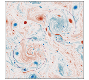
A snapshot of the vorticity from a simulation of the Lofoten Basin, from Trodahl et al. (Reference Trodahl, Isachsen, Lilly, Nilsson and Melsom Kristensen2020), is shown in figure 1. The Lofoten vortex is in the centre, near the Greenwich meridian at 72N. This merges with other anticyclones and is coherent over the entire eight year simulation. However the surface flow is remarkably turbulent, with vortices of both signs present. The cyclones also merge, but are preferentially strained out and do not grow in size. This yields a distinct asymmetry in the vortex evolution. Such an asymmetry is unusual for balanced (quasi-geostrophic) flows, and ageostrophic effects are usually invoked to explain such differences (e.g. Polvani et al. Reference Polvani, McWilliams, Spall and Ford1994; Graves, McWilliams & Montgomery Reference Graves, McWilliams and Montgomery2006). Moreover, the vortices in the figure are not isolated. Thus, self-propagation, which is due to the spin up of secondary ‘beta gyres’ near the bottom (e.g. LaCasce Reference LaCasce1998), would likely be overwhelmed by interactions with nearby vortices at the surface.

Figure 1. The surface relative vorticity from a high-resolution simulation of the Lofoten Basin (§ 4). The figure is rotated so that west is upward. The flow is significantly turbulent and a prominent anticyclone is seen near the basin centre. The isobaths are shown in black for every 1000 m and the contours show the Rossby number, i.e. the relative vorticity normalized by the Coriolis parameter,  $f$. The solid contours are the isobaths, in 500 m increments.
Hereafter we revisit the theory relevant to a turbulent flow over a depression. A variational solution in two layers predicts a cyclonic flow resembling the topography, as in the barotropic case. The flow is steady and bottom intensified, as seen in previous studies with continuous stratification (Merryfield Reference Merryfield1998; Venaille, Vallis & Smith Reference Venaille, Vallis and Smith2011). The surface potential vorticity (PV) is anticyclonic and strongest at intermediate energies. Thereafter, we test the predictions using solutions from an idealized (quasi-geostrophic) model and a full complexity general circulation model.
2. Theory
In 2-D turbulence, energy cascades to larger scales while enstrophy cascades to smaller (Fjørtoft Reference Fjørtoft1953; Kraichnan Reference Kraichnan1967). Thus, small-scale dissipation preferentially removes enstrophy while energy is approximately conserved. Bretherton & Haidvogel (Reference Bretherton and Haidvogel1976) proposed that 2-D turbulence should therefore evolve to a state with minimum enstrophy while conserving energy. With bathymetry the predicted flow is correlated with topography, as follows.
2.1. Single layer
For a barotropic (single layer), quasi-geostrophic (QG) flow, the motion is governed by
 \begin{equation} \frac{\partial}{\partial t} \zeta + J(\psi,\zeta+h) = 0 ,\end{equation}
where  $J(a,b)$ is the Jacobian operator and
  $\zeta$ the relative vorticity,
 \begin{equation} \zeta=\nabla^2 \psi \end{equation}
(Pedlosky Reference Pedlosky1987). Here  $\psi$ is the geostrophic streamfunction and
  $h=f L h_b/(U H)$ is the scaled bottom elevation, with
  $f$ the Coriolis parameter (assumed constant),
  $L$ the lateral domain scale,
  $H$ the mean depth of the layer,
  $U$ the velocity scale and
  $h_b$ the dimensional topographic height. Equation (2.1) admits a set of conserved quantities, one of which is the potential enstrophy
 \begin{equation} \iint Z \, {\rm d}\,A \equiv \iint \frac{1}{2}(\zeta +h)^2 \, {\rm d}\,A , \end{equation}
and the other the kinetic energy
 \begin{equation} \iint E \, {\rm d}\,A \equiv \iint \frac{1}{2} |\boldsymbol{\nabla} \psi|^2 \, {\rm d}\,A . \end{equation}
Bretherton & Haidvogel (Reference Bretherton and Haidvogel1976) defined a functional
 \begin{equation} \mathcal{L} = \iint Z + \lambda (E-E_0) \, {\rm d}\,A, \end{equation}
where  $\lambda$ is a Lagrange multiplier. By minimizing this they obtained enstrophy extrema subject to the constraint that the energy equals its initial value,
  $E_0$. The first variation of
  $\mathcal {L}$ is given by
 \begin{equation} \delta \mathcal{L} = \iint (\zeta+h) \delta \zeta + \lambda \delta E \, {\rm d}\,A = 0 . \end{equation}
Following integration by parts, this reduces to
 \begin{equation} \iint \nabla^2[\nabla^2 \psi +h - \lambda \psi] \delta \psi \, {\rm d}\,A = 0. \end{equation}
This yields an Euler–Lagrange equation
 \begin{equation} \nabla^2 \psi - \lambda \psi ={-} h .\end{equation}
Assuming a doubly periodic domain, one can Fourier transform the streamfunction and bathymetry, i.e.
 \begin{equation} (\psi,h)=\sum_{k,l} (\hat \psi, \hat h) \,{\rm exp}({\rm i}kx+{\rm i}ly). \end{equation}
Then the solution to (2.8) is
 \begin{equation} \hat \psi = \sum_{k,l} \frac{\hat h}{K^2 + \lambda} ,\end{equation}
where  $K^2=k^2+l^2$. If
  $\lambda > 0$, the streamfunction is a low-pass filtered representation of the bathymetry,
  $h$, with cyclonic flow over depressions and anticyclonic flow over seamounts. If
  $\lambda < 0$, the flow can be reversed and singularities occur (Carnevale & Frederiksen Reference Carnevale and Frederiksen1987; LaCasce, Nøst & Isachsen Reference LaCasce, Nøst and Isachsen2008).
The second variation of  $\mathcal {L}$ can be shown to be
 \begin{equation} \delta^2 \mathcal{L} = \frac{1}{2} \iint (\nabla^2 \delta \psi)^2 + \lambda |\boldsymbol{\nabla} \delta \psi |^2 \, {\rm d}\,A . \end{equation}
Expanding the perturbation  $\delta \psi$ also in a Fourier series yields
 \begin{equation} \delta^2 \mathcal{L} = \frac{1}{2} \sum_{k,l} K^2(K^2+\lambda) |\delta \hat \psi|^2 . \end{equation}
This is positive definite if  $\lambda >-K^2_{min}$, indicating a minimum enstrophy solution (Carnevale & Frederiksen Reference Carnevale and Frederiksen1987). Solutions with smaller
  $\lambda$ are saddle points, such that the second variation can be positive or negative, depending on the wavenumber (e.g. Gray & Taylor Reference Gray and Taylor2007).
The minimum enstrophy solution is steady, as any such solution to (2.1) has
 \begin{equation} \zeta + h =\mathcal{F}(\psi) , \end{equation}
where  $\mathcal {F}$ is a function. Assuming the linear relation
  $\mathcal {F}=\lambda \psi$ yields the solution in (2.10). The solution is also nonlinearly stable. Carnevale & Frederiksen (Reference Carnevale and Frederiksen1987) demonstrated this by defining a norm based on the enstrophy and energy, identical to the second variation in (2.12). That this is positive for
  $\lambda > -K_{min}^2$ indicates that arbitrary perturbations, no matter how large, cannot grow in time.
The solution with  $\lambda =1$ is shown in figure 2. The bathymetry (upper left panel) is an elliptical depression, given by
 \begin{equation} h=h_0 \exp\left[-\left(\frac{x}{1.5}\right)^2-y^2\right] , \end{equation}
with  $h_0=-1$. The relative vorticity (upper right) is positive and about half as strong, so that the total vorticity,
  $\zeta + h$, is negative (lower left). The streamfunction is also negative (lower right), corresponding to cyclonic flow. It is more circular than the depression, indicating the flow crosses the isobaths. However, the streamfunction is identical to the total PV,
  $\zeta + h$ (lower left), as expected with
  $\lambda =1$.

Figure 2. Single-layer minimum enstrophy solution for an elliptical depression with  $\lambda =1$. The bathymetry is plotted in the upper left panel, the relative vorticity in the upper right, the total PV (the sum of the relative vorticity and topography,
  $h$) in the lower left and the streamfunction in the lower right. The domain is
  $2 {\rm \pi}\times 2 {\rm \pi}$, so that
  $K_{min}=1$.
The Lagrange multiplier,  $\lambda$, is determined by the total (kinetic) energy, given by
 \begin{equation} KE = \frac{1}{2} \sum_{k,l} \frac{K^2 |\hat h|^2}{(K^2 + \lambda)^2} .\end{equation}
The dependence on  $\lambda$ is shown in the left panel of figure 3. The figure closely resembles those of Carnevale & Frederiksen (Reference Carnevale and Frederiksen1987) and LaCasce et al. (Reference LaCasce, Nøst and Isachsen2008). The kinetic energy decreases monotonically for positive
  $\lambda$ and exhibits singularities for negative values (at wavenumbers where the denominator of (2.15) is zero). As the domain scale is
  $2 {\rm \pi}\times 2 {\rm \pi}$, these occur at integer wavenumbers, with
  $K_{min}=1$.

Figure 3. (a) Total energy as a function of  $\lambda$ for the solution shown in figure 2. (b) A cross-section in the middle of the depression of the total PV,
  $\zeta +h$, for different
  $\lambda$. Note that
  $K_{min}=1$.
The value of  $\lambda$ also affects the PV. Cross-sections of
  $\zeta +h$ for various
  $\lambda$ are plotted in the right panel of figure 3. With large positive
  $\lambda$, the relative vorticity is less than
  $h$ and the latter dominates the total PV. As
  $\lambda \rightarrow 0$, the vorticity is comparable to
  $h$ and of opposite sign, so that the total PV is approximately constant, i.e. it is homogenized (also noted by Siegelman & Young Reference Siegelman and Young2023). With
  $-K_{min}^2<\lambda <0$, the PV is positive and dominated by the relative vorticity. As
  $\lambda$ approaches
  $-K_{min}^2$, the PV increases without bound, in tandem with the energy.
2.2. Two layers
Now consider the case with two fluid layers. Under the QG approximation, the layer potential vorticities evolve according to (Pedlosky Reference Pedlosky1987; Vallis Reference Vallis2006)
 \begin{equation} \frac{\partial}{\partial t} q_1 + J(\psi_1,q_1) = 0, \quad \frac{\partial}{\partial t} q_2 + J(\psi_2,q_2 +h) = 0,\end{equation}
with the perturbation PVs given by
 \begin{equation} q_{1}=\nabla^2 \psi_1 + F_1(\psi_{2} - \psi_1), \quad q_2= \nabla^2 \psi_2 + F_2(\psi_1 -\psi_2). \end{equation}
The PVs are a combination of the ‘relative vorticity’ in the layer and the ‘stretching vorticity’, which is proportional to the layer interface displacement. Here
 \begin{equation} F_i=\frac{f^2 L^2}{g' H_i} \end{equation}
are inverse Burger numbers, with  $g'=(\rho _2-\rho _1)g/\rho _0$ the ‘reduced gravity’ and
  $H_i$ the undisturbed layer depths. The
  $F_i$ are the squared non-dimensional ratio between the domain scale and the ‘deformation radius’,
  $\sqrt {g'H_i}/f$, in the corresponding layer.
From (2.16a,b), it can be shown that total energy is conserved. This is a combination of the layer kinetic and potential energies,
 \begin{equation} \iint E \, {\rm d}\,A \equiv \frac{1}{2} \iint [\gamma_1 |\boldsymbol{\nabla} \psi_1|^2 +\gamma_2 |\boldsymbol{\nabla} \psi_2|^2 + F (\psi_1-\psi_2)^2] \, {\rm d}\,A, \end{equation}
where  $\gamma _i=H_i/(H_1+H_2)$ are relative layer depths and
  $F \equiv F_1 + F_2 = f^2 L^2 (H_1 + H_2)/(g' H_1H_2)$.
We minimize the total enstrophy while conserving total energy. To this end, we employ the functional
 \begin{equation} \mathcal{L} = \iint \frac{\gamma_1 q_1^2}{2} + \frac{\gamma_2 (q_2+h)^2}{2} + \lambda (E-E_0) \, {\rm d}\,A . \end{equation}
Note the layer potential enstrophies, the first two terms, are weighted by the respective layer depths. The first variation of  $\mathcal {L}$ is
 \begin{equation} \delta \mathcal{L} = \iint \gamma_1 q_1 \delta q_1 + \gamma_2 q_2 \delta q_2 + \lambda \delta E \, {\rm d}\,A = 0 . \end{equation}
Integrating the energy term by parts, this can be rewritten as
 \begin{equation} \delta \mathcal{L} = \iint \gamma_1 (q_1 - \lambda \psi_1) \delta q_1 + \gamma_2 (q_2 + h - \lambda \psi_2) \delta q_2 \, {\rm d}\,A = 0 . \end{equation}
Thus, the Euler–Lagrange equations are simply
 \begin{equation} q_1 = \lambda \psi_1, \quad q_2 + h = \lambda \psi_2 . \end{equation}
As in the single-layer case, the condition for minimum enstrophy is equivalent to that for a steady state of the PV equations (2.16a,b); again, the variational solutions are also steady solutions.
The solutions are obtained from (2.23a,b), using the PV definitions (2.16a,b). After Fourier transforming, we have
 $$\begin{gather} -(K^2+F_1+\lambda) \hat \psi_1 + F_1 \hat \psi_2 = 0 , \end{gather}$$
 $$\begin{gather}F_2 \hat \psi_1 - (K^2+F_2+\lambda) \hat \psi_2 ={-} \hat h . \end{gather}$$
Multiplying the first equation by  $\gamma _1$ and the second by
  $\gamma _2$ and adding yields
 \begin{equation} \psi_B \equiv \gamma_1 \psi_1 + \gamma_2 \psi_2 = \frac{\gamma_2 \hat h}{K^2 + \lambda} , \end{equation}
where  $\psi _B$ is the ‘barotropic streamfunction’, representing the depth-averaged flow. Thus, the barotropic solution is very similar to that from the single-layer derivation (2.10). Subtracting the equations instead yields the baroclinic streamfunction
 \begin{equation} \psi_T \equiv \psi_1 - \psi_2 ={-} \frac{\hat h}{K^2 + F+ \lambda} . \end{equation}
This has the opposite sign as the topographic perturbation, implying the solution is bottom intensified if the denominator is positive.
In terms of the layer streamfunctions, the solution can be obtained from (2.25) using Cramer's rule
 \begin{equation} \hat \psi_1 = \frac{F_1 \hat h}{\triangle}, \quad \hat \psi_2 = \frac{(K^2 + \lambda + F_1) \hat h}{\triangle}, \end{equation}
with
 \begin{equation} \triangle= (K^2+\lambda)(K^2 + F + \lambda) .\end{equation}
The potential vorticities are then proportional to the streamfunctions, from (2.23a,b). Again, the solution is bottom intensified if  $\triangle$ is positive.
In addition, the second variation of  $\mathcal {L}$ can be shown to be
 \begin{align} \delta^2 \mathcal{L} &= \frac{1}{2} \sum_{k,l} |F_1 \delta \hat \psi_2 -(K^2 +F_1) \delta \hat \psi_1|^2 + |F_2 \delta \hat \psi_1 -(K^2 +F_2) \delta \hat \psi_2|^2 \nonumber\\ &\quad + \lambda [\gamma_1 K^2 |\delta \hat \psi_1|^2 + \gamma_2 K^2 |\delta \hat \psi_2|^2 + F|\delta \hat \psi_1- \delta \hat \psi_2|^2] . \end{align}
While more complicated than in the single-layer case, the right-hand side is clearly positive if  $\lambda >0$. As in the single-layer case, one can define a norm based on the potential enstrophies and the energy, following Carnevale & Frederiksen (Reference Carnevale and Frederiksen1987). The result is the same, indicating the steady solutions are stable if
  $\lambda$ is positive.
The two-layer solution with  $\lambda =1$ is plotted in figure 4. The bathymetry is the same elliptical depression used for figure 2. The inverse Burger numbers are
  $F_1=25$ and
  ${F_2=6.25}$, so that the domain is five times the surface deformation radius and the layer depth ratio,
  $H_1/H_2=1/4$. The latter is preferable to having equal layer depths, which excludes a particular triad interaction (Flierl Reference Flierl1978); the chosen value is comparable to the typical depth ratio in the ocean.

Figure 4. Two-layer minimum enstrophy solution for an elliptical depression with  $F_1=25$,
  $F_2=6.25$ and
  $\lambda =1$. The relative vorticities are in the left panels and the potential vorticities in the right panels.
Shown are the relative vorticities (left panels) and the potential vorticities (right) (the streamfunctions are not plotted but are identical to the PVs). The flow is bottom intensified, but the surface flow is nearly as strong as that at depth. This is because the depression is significantly larger than the deformation radius; with smaller depressions the surface flow is weaker. The bottom-intensified solution is in line with previous studies with continuous stratification (Merryfield Reference Merryfield1998; Venaille Reference Venaille2012).
The perturbation PV in the lower layer (not shown) is positive and primarily reflects the relative vorticity (lower left). Nevertheless, the total PV, dominated by the topographic contribution, is negative. The surface PV (upper right panel) is also negative and nearly as strong as that at depth. However, this is due to the stretching term,  $F_1(\psi _2-\psi _1)$, which is larger because the upper layer is thinner (
 $F_1$ is four times larger than
  $F_2$). As such, the PV does not change sign in the vertical, signifying the flow is baroclinically stable (Pedlosky Reference Pedlosky1987).
The deep PV (right panel of figure 5) varies with  $\lambda$ as in the single-layer case. For large
  $\lambda$, the PV is negative and dominated by topography while with
  $-K_{min}^2<\lambda < 0$ it is positive and dominated by the cyclonic relative vorticity. With
  $\lambda$ near zero the two contributions approximately cancel and the total PV is homogenized.

Figure 5. Cross-sections in the middle of the depression of the upper layer PV (a) and the lower layer PV(b) for different  $\lambda$, and
  $F_1=25$ and
  $F_2=6.25$.
The surface PV on the other hand exhibits a non-monotonic dependence on  $\lambda$ (left panel of figure 5). For large positive
  $\lambda$, the PV is near zero and the surface flow is weak. Decreasing
  $\lambda$, the PV becomes more negative, reaching a minimum near
  $\lambda =10$. As
  $\lambda$ approaches zero, the PV becomes homogenized. Thus, the surface PV is most pronounced at intermediate values of positive
  $\lambda$. For negative
  $\lambda$, the surface PV is positive and increases indefinitely as
  $\lambda$ approaches
  $-K_{min}^2$.
It is useful to compare these fields with those of topographic waves. Bottom intensification is a signature of the latter, but the waves have a surface PV that is identically zero (LaCasce Reference LaCasce1998). It can be shown that the surface flow of the minimum enstrophy solution is somewhat weaker. The surface PV will be a central concern when discussing the numerical results below.
As before, the Lagrange multiplier determines the energy (figure 6). This closely resembles the single-layer case, with the energy decreasing monotonically for positive  $\lambda$ and exhibiting singularities for negative values, where
  $\triangle$ in (2.29) is zero. There are evidently two sets of singularities, for
  $\lambda$ greater and less than roughly
  $-30$. Those with larger
  $\lambda$ are associated with the barotropic modes and the others with the baroclinic modes. Though the solutions are provably enstrophy minima for
  $\lambda >0$, from (2.30), it is plausible that all the solutions with
  $-K_{min}^2<\lambda <0$ are minima as well, as in the one-layer case.

Figure 6. Total energy for the two-layer minimum enstrophy solution as a function of  $\lambda$ with
  $F_1=25$ and
  $F_2=6.25$.
To summarize, the two-layer solutions with positive  $\lambda$ are largely consistent with the single-layer case, with cyclonic flow in a depression and anticyclonic flow over a seamount. The flow is bottom intensified, as in previous studies with continuous stratification (Merryfield Reference Merryfield1998; Venaille Reference Venaille2012), and the bottom PV is homogenized as
  $\lambda \rightarrow 0$. The flow also has negative PV at the surface (over a depression); this is homogenized both for large
  $\lambda$ and at
  $\lambda =0$. The surface PV is strongest with positive
  $\lambda$ at intermediate energies.
3. Quasi-geostrophic simulations
We now consider simulations using a QG model, with one and two layers. The model solves (2.1) and (2.16a,b), respectively, with a doubly periodic domain and  $N = 512$ grid points in both lateral directions. The code is implemented with the GeophysicalFlows.jl pseudo-spectral package (Constantinou et al. Reference Constantinou, Wagner, Siegelman, Pearson and Palóczy2021). Time stepping is with a fourth-order Runge–Kutta scheme and an exponential filter is employed to remove enstrophy near the grid scale (Canuto et al. Reference Canuto, Hussaini, Quarteroni and Zang1988). Total energy is conserved to within 0.5 % in all cases. The flow is initialized with a random perturbation PV that is barotropic, surface trapped or bottom trapped, with specified initial energies. The initial perturbations are derived from a uniform (white) spectrum with random phases. The spectrum is truncated between two wavenumbers
  $K_l$ and
  $K_r$. Various
  $K_l$ and
  $K_r$ were tested, but the results shown hereafter are based on runs with
  $K_l = 4$ and
  $K_r = 10$ (the deformation wavenumber in the two-layer experiments is
  $K = 11$). Both the late time flow and energy spectra were insensitive to this choice, and it minimized energy dissipation across all experiments.
The bathymetry consists of a depression and a seamount, of identical dimensions. We examine both symmetric (circular) and asymmetric (elliptical) features. Specifically, the topographic height  $h$ is given by
 \begin{align} h &= h_0 \exp[-(x - x_{0s})^2/(2\sigma_x^2) -(y - y_{0s})^2/(2\sigma_y^2)]\nonumber\\ &\quad - h_0 \exp[-(x - x_{0b})^2/(2\sigma_x^2) -(y - y_{0b})^2/(2\sigma_y^2)] , \end{align}
where  $h_0 = 3$,
  $\sigma _x$ and
  $\sigma _y$ are respectively the semi-major and semi-minor axes (
 $\sigma _x = \sigma _y$ for the circular topography simulations). The centres of the depression and elevation are given respectively by (
 $x_{0b}$,
  $y_{0b}$) and (
 $x_{0s}$,
  $y_{0s}$). In discussing the results we focus primarily on the depression, for brevity. The situation over the seamount is qualitatively the same but with the circulations reversed. All experiments are performed on the
  $f$ plane. The single-layer experiments (figures 7, 8 and 10) all have an initial energy of
  $E=0.05$. Different initial conditions and energies are employed in the two-layer experiments, as listed in table 1 below.
Table 1. Initial conditions for the two-layer QG experiments with corresponding figure numbers. The dashes indicate the fields were calculated from the specified PV or streamfunctions.


Figure 7. Evolution of the flow in a single-layer circular depression at early (top row) and late (bottom row) times. The former is at roughly one advective time scale,  $T=L/U$, and the latter at about 30
  $T$. The energy is
  $E=0.05$. Left column: relative vorticity; right column: streamfunction. The maximum topographic height is
  $h=\pm 3.0$ and the ellipse axes are
  $\sigma _x=\sigma _y=0.7$. The solid and dashed circles indicate the
  $h=-0.5$ and
  $h=0.5$ contours, respectively.

Figure 8. As in figure 7, but for an elliptical depression. The topographic height is the same, but now  $\sigma _x=1.4=2 \sigma _y$.
3.1. Single layer
Shown in figure 7 are snapshots of the relative vorticity and streamfunction for a single-layer simulation, with a circular depression and seamount. The ellipse axes are  $\sigma _x=\sigma _y=0.7$. The depression lies in the lower left of the panels and the seamount in the upper right. The upper panels are from early in the simulation and the lower from a late phase, after the flow has settled into a statistically stationary state.
Early on, vortices merge throughout the domain. Significantly, there is an asymmetry between cyclones and anticyclones. Over the depression, the cyclones (in red) are strained out while the anticyclones (blue) retain an approximately axisymmetric shape. At the late stage there is a large-scale cyclonic flow with a single anticyclone at the centre (lower left panel). The cyclonic flow dominates the streamfunction, while the anticyclone is barely visible (lower right panel). As noted, the situation over the seamount is similar, but with the circulations reversed.
The streamfunctions agree qualitatively with those of Bretherton & Haidvogel (Reference Bretherton and Haidvogel1976). However they did not observe the central anticyclone, most likely as their simulations were of low resolution ( $64 \times 64$ grid points). When we used the same resolution, the anticyclones were lost to dissipation. The solution agrees well though with those described by Solodoch et al. (Reference Solodoch, Stewart and McWilliams2021), who found both the cyclonic circulation and the strong anticyclone in the centre, across a range of simulations with a circular depression.
The corresponding fields for an elliptical depression and seamount are shown in figure 8. The semi-major axis in this case is twice the semi-minor, with  $\sigma _x=1.4$ while
  $\sigma _y=0.7$. Again the mergers are asymmetric, with the cyclonic vortices preferentially sheared out over the depression. But in contrast with the circular depression, the final central anticyclone is much smaller and weaker (lower left panel). As such, the result is even more sensitive to model resolution. With
  $256^2$ grid points, the anticyclone appeared less often, and was rarely observed with
  $128^2$ grid points. In the high-resolution simulations with different random initial conditions, we sometimes found two small vortices orbiting the centre or no central anticyclone at all, but cases with a strong anticyclone were rare.
Why do the symmetric and asymmetric basins differ? With a single layer and radially symmetric topography, angular momentum is conserved in the absence of lateral fluxes (Nycander & LaCasce Reference Nycander and LaCasce2004):
 \begin{equation} \frac{{\rm d}}{{\rm d} t} \iint r^2 (\zeta + h) \, {\rm d}\,A = 0. \end{equation}
Thus, if the angular momentum is nearly zero initially, a cyclonic circulation would have to be balanced by an anticyclonic flow in the interior. In reality there are lateral fluxes and these alter the net circulation, as seen next. But the fact remains that a symmetric depression is probably a special case.
The cyclonic circulation spins up at the expense of the cyclonic vortices strained out during mergers, but cross-boundary vorticity fluxes also contribute, as noted above. Integrating (2.1) over a region bounded by an outer isobath (the  $h=0.05$ contour, indicated by the solid ellipse in figure 8) and in time, we have
 \begin{equation} \iint \zeta(t) - \zeta(0) \, {\rm d}\,A + \int \, {\rm d} t \oint \zeta {\boldsymbol{u}} \boldsymbol{\cdot} \hat n \, {\rm d} l = 0 . \end{equation}
The two terms are plotted in figure 9. The circulation, initially near zero, is briefly negative before the cyclonic (positive) circulation is established at roughly  $t=80$. The integrated flux mirrors this, with an initially positive flux followed by a negative one. The latter primarily reflects an inward drift of cyclones.

Figure 9. The PV budget terms in the single-layer elliptical depression experiment (figure 8) as the flow approaches the final state. The blue and red curves are respectively the area-integrated vorticity (the circulation) and the time-integrated vorticity flux across an isobath bounding the depression.
Such a drift is contrary to the behaviour of solitary cyclones, which tend to propagate out of a depression (Carnevale et al. Reference Carnevale, Kloosterziel and Van Heijst1991). The net convergence of cyclones here occurs because they are preferentially strained out during mergers. As such, there is a ‘sink’ for cyclonic vortices in the depression; those that enter often do not leave. This is not the case with anticyclones, which survive the mergers and can exit the depression again.
Whether the central anticyclone is trapped in the depression depends on the PV; consistent with the minimum enstrophy solution, the PV becomes homogenized for more energetic flows. Shown in figure 10 are two cases, one with  $E=0.05$ (left panel) and one with a kinetic energy ten times larger (right panel). As seen in the inserts, the total PV is negative with
  $E=0.05$, but near zero with
  $E=0.5$. In the former case, an anticyclone/cyclone settles in the middle of the depression/seamount while in the high energy case, the vortices move freely about, as over a flat bottom. Thus, having PV gradients in the depression is essential to trapping the anticyclone, as would be expected with self-propagation of the vortex (§ 5).

Figure 10. Late time snapshots of total PV  $\zeta + h$, with the circular depression in single-layer experiments with
  $E=0.05$ (a) and
  $E=0.5$ (b). The relative and total PV across the centre of the depression (as indicated by the dashed line) are shown in the inserts.
Interestingly, the PV is homogenized at the largest energies, corresponding to the  $\lambda =0$ minimum enstrophy solution. Cases corresponding to the range
  $-K_{min}^2 <\lambda <0$, in which the cyclonic relative vorticity exceeds the topographic contribution, were never observed. So it appears only the positive
  $\lambda$ solutions are relevant for the simulations.
Lastly, consider the  $q-\psi$ relation, shown for the elliptical depression case in figure 11. The dependence is nearly linear, approximately obeying
 \begin{equation} q \approx 2.7 \psi . \end{equation}
This too is consistent with the minimum enstrophy solution. The central anticyclone and cyclone contribute only by producing the sharp deviations seen at the extremes of the distribution.

Figure 11. A scatterplot for the total PV versus the streamfunction in the single-layer, elliptical depression case with  $E=0.05$.
3.2. Two layers
Now consider the two-layer case. We restrict attention to the elliptical depression and seamount, and set the parameters so that the domain scale is roughly 10 times the surface deformation radius and the layer depth ratio is 1/4. The different experiments are summarized in table 1.
We begin with experiments in which the perturbation PV in the lower layer,  $q_2$, is random and that in the upper layer,
  $q_1$, is zero. In these, the bottom layer evolves as before, with cyclones preferentially strained out in the depression as the cyclonic topographic flow spins up (figure 12). In the final state, a small anticyclone remains in the centre (bottom left panel), as with a single layer (figure 8).

Figure 12. Late time configuration of the flow in two layers with initially random  $q_2$ and
  $q_1=0$. (a) Surface PV, (b) surface streamfunction, (c) bottom PV, (d) bottom streamfunction.
The surface streamfunction (upper right panel of figure 12) indicates cyclonic circulation above the depression, somewhat weaker than that at depth (lower right). The surface PV (upper left) is nearly zero, as required from the conservation of upper layer PV. Thus, the vertical structure of the mean flow is that of topographic waves. As noted, this differs from the minimum enstrophy solution, which has negative surface PV, but it is straightforward to obtain a minimum enstrophy solution with zero surface PV imposed. This yields a nearly identical flow (not shown).
The PV fluxes can be obtained by integrating (2.16a,b) over an area bounded by an isobath, i.e.
 \begin{equation} \iint q_j(t) - q_j(0) \, {\rm d}\,A + \int \, {\rm d} t \oint q_j {\boldsymbol{u}}_j \boldsymbol{\cdot} \hat n \,{\rm d} l = 0 , \end{equation}
where the index,  $j=1,2$, indicates the layer. The surface fluxes are necessarily near zero, while those in the lower layer (not shown) closely resemble the fluxes in the single layer. Thus, again the net cyclonic circulation over the depression is supported by a net influx of cyclones.
As with a single layer, the  $q_2+h-\psi _2$ scatterplot (blue curve in the left panel of figure 13) is nearly linear with a positive slope. The
  $q_1-\psi _1$ curve instead lies mostly along the
  $q_1=0$ axis, with small deviations due to numerical noise.

Figure 13. Scatterplots of the total layer PVs versus the streamfunctions for the simulations with initially bottom-trapped (a) and surface-trapped PV (b).
Thus, the bottom-trapped PV case is very similar to that with a single layer, with a bottom-intensified cyclonic circulation dominating the flow and the upper layer largely passive.
The evolution with an initially surface-trapped PV is somewhat different. Shown in figure 14 are the fields that result with a random initial  $q_1$, with
  $q_2=0$. A bottom-intensified cyclonic flow spins up, but no central anticyclone forms over the depression. Because
  ${q_2=0}$ initially, the anticyclones that form are weak and do not survive. Instead, and strikingly, a large anticyclone appears at the surface.

Figure 14. As in figure 12, but for an initially random surface PV.
Vortices form initially at the surface and merge actively thereafter. The surface vortices are approximately deformation scale and ‘compensated’, i.e. they have no deep flow. As such, their horizontal flow does not extend far beyond the PV contours (upper panels of figure 14). This is as expected for vortices above a resting lower layer (e.g. Flierl et al. Reference Flierl, Larichev, McWilliams and Reznik1980; Larichev & McWilliams Reference Larichev and McWilliams1991). As is typical in 2-D turbulence simulations, only a dipole remains at the end, but here with the anticyclone trapped over the depression and the cyclone over the seamount.
The vortex mergers are again asymmetric, but in a different way than before. After the cyclonic flow spins up, only anticyclones merge over the depression. The cyclones enter and leave, but merge instead outside, and over the seamount. Thus, there is a sink for surface anticyclones over the depression. Notably though, the cyclones are not strained out as the bottom-intensified flow spins up (animations are available in the supplementary movies available at https://doi.org/10.1017/jfm.2023.1084).
The potential circulation over the depression and integrated PV fluxes are shown in figure 15. The evolution in the lower layer (b) resembles that with a single layer, with a strengthening cyclonic circulation (blue curve) balanced by negative PV fluxes (red curve). As before, cyclones enter the depression and are lost to the large-scale circulation. The circulation in the upper layer (blue curve, left panel) evolves more sporadically, reflecting the motion of individual vortices. It eventually hovers around a negative value, due to the lone central anticyclone. The integrated flux is accordingly positive, consistent with a net inward drift of anticyclones. Significantly, the surface circulation is consistently negative only after the deep flow is established (by roughly  $t=200$ in the figure). This suggests the merger asymmetry is related to the cyclonic flow.

Figure 15. As in figure 9, but for the upper (a) and lower (b) layers in the experiment with initially surface-trapped PV.
The  $q_2+h-\psi _2$ curve is linear with a positive slope, as in the bottom-trapped PV case (left panel of figure 13). However, the surface layer curve (in red) exhibits two regions with negative slopes. These correspond to the two surface vortices, a negative one over the depression and a positive one over the seamount.
As in the single-layer case, vortex trapping is dependent on the total energy. The late stage PV for three cases with an initially surface-trapped PV are shown in figure 16. The initial energies are  $E=0.0125$,
  $0.05$ and
  $1.0$. In all three cases,
  $q_1$ is dominated by solitary vortices. With
  $E=0.05$, a cyclone is trapped over the seamount and two anticyclones over the depression (these subsequently merge). In contrast, with
  $E=0.0125$ the vortices are less confined; the cyclone lingers near the seamount, while the anticyclone moves about the domain. The same is true with
  $E=1.0$, as both vortices move freely about the domain. Thus, trapping occurs primarily at intermediate energies.

Figure 16. Late time snapshots of layer total PVs with an elliptical depression in two-layer experiments with an initially surface-trapped PV. The initial energies are  $E=0.0125$ (a,d),
  $E=0.05$ (b,e) and
  $E=0.5$ (c, f). The insets show
  $q_1$,
  $q_2$ and
  $q_2 + h$ distributions across the middle of the depression, indicated by the horizontal dashed line on panels (a–f). Results are shown for (a)
  $q_1, E = 0.0125$; (b)
  $q_1, E = 0.05$; (c)
  $q_1, E = 1.0$;(d)
  $q_2, + h, E = 0.0125$; (e)
  $q_2, + h, E = 0.05$ and ( f)
  $q_2, + h, E = 1.0$.
The free motion at large energies, as in the single-layer case, happens because the PV in both layers is homogenized. The latter is seen in the PV slices shown in the inserts in figure 16(c, f). This is as expected for the minimum enstrophy solution with  $\lambda \approx 0$. The (nearly) free motion at the weakest energy is unexpected though. In this case the deep PV, dominated by topography, is strongly negative (figure 16d), which should favour vortex self-propagation. Perhaps most noticeably, the surface PV over the depression is near zero outside the vortices in all three cases. This is a striking deviation from the minimum enstrophy prediction.
Evidently the surface vortices disrupt the formation of the large-scale surface PV. The latter is seen however in simulations with more quiescent vortex fields. Two examples, with surface-trapped initial flows that follow the isobaths, are shown in figure 17. The circulation over the depression is anticyclonic in one experiment and cyclonic in the other. In both cases, energy is transferred to the lower layer, yielding the large-scale cyclonic flow and a lone anticyclone in the centre (upper right). But a large-scale negative PV also appears. This is also true when the surface flow is initially cyclonic (lower panels of figure 17). Then the cyclones shift to the seamount and the anticyclones to the depression. But in both cases, the less energetic vortices permit the formation of a large-scale surface PV.

Figure 17. Two simulations with initially surface-trapped flow over an elliptical depression and seamount. Here,  $\psi _1$ initially follows the bathymetry and
  $\psi _2=0$. The initial perturbation PVs are shown on the left and the final PVs on the right; the top/bottom rows show the surface/bottom fields, respectively. Note the domain is
  $4 {\rm \pi}\times 4 {\rm \pi}$. The solid and dashed circles indicate the
  $h=-0.02$ and
  $h=0.02$ contours, respectively, and the initial energy is
  $E=0.05$. (a) Anticyclone
  $q_1$, initial; (b) anticyclone
  $q_1$, late; (c) cyclone
  $q_1$, initial and(d) cyclone
  $q_1$, late.
The symmetric depression differs in these experiments as well. If one starts with a surface-trapped flow with negative PV over a circular depression, the flow does not evolve at all (not shown). Indeed, such a flow is a stable steady state if the bathymetry is symmetric.
Additional experiments were made with an initially barotropic PV as well (not shown). In these, the evolution is essentially a combination of the initially surface- and bottom-trapped PV cases above. Most strikingly, the vortex evolution is independent in the layers. Thus, there is no alignment of like-signed features in the layers, as occurs over a flat bottom (McWilliams Reference McWilliams1990). Lone anticyclones form over the depression in both layers, but the surface vortex is smaller than in the initially surface-trapped case due to more active straining by the stronger cyclonic flow. Otherwise, the results are consistent with those described above.
4. Primitive equation model
The preceding simulations and the minimum enstrophy solutions are based on the two-layer QG equations. To see to what extent the results apply in a more realistic environment, we employ a full complexity ocean model. This allows testing configurations (e.g. finite amplitude interfacial and topographic deviations) beyond the formal requirements of QG.
The simulations were performed with the coastal and regional ocean community (CROCO) version of the regional ocean modelling system (ROMS; Shchepetkin & McWilliams Reference Shchepetkin and McWilliams2005; Haidvogel et al. Reference Haidvogel2008).
The simulations were run with a constant Coriolis parameter,  $f=1.37\times 10^{-4}$ s
 $^{-1}$ and density is determined solely by temperature, for simplicity. The background temperature stratification was set to an exponential profile,
  $T = T_s \exp (z/h_e)$, with
  $h_e\approx 400$ m. The buoyancy frequency,
  $N$, was chosen so that the (flat bottom) deformation radius,
  $L_d \approx \int _{-H}^{0}{N\, {\rm d} z/f{\rm \pi} }$ (Chelton et al. Reference Chelton, DeSzoeke, Schlax, El Naggar and Siwertz1998), was roughly 20 km. A random perturbation was added to the initial density field, with corresponding (balanced) velocities obtained by integrating the thermal wind relation from the bottom. The perturbation was surface intensified, with an e-folding scale equal to that of the background stratification,
  $h_e$. Spin down experiments were run for 5–7 years. In the simulations with bottom drag, quadratic friction with a drag coefficient
  $C_d=10^{-3}$ was used.
The model geometry is a doubly periodic square box with sides  $L = 1205$ km, and a lateral grid spacing of 5 km. We examine an isolated elliptical depression and random topographic relief. The former is a Gaussian-shaped depression
  $600$ m deep, surrounded by a flat region
  $1500$ m deep. For the random relief, a Gaussian random field with an amplitude of
  $100$ m was added to a mean depth of
  $D=1900$ m. The resulting depth perturbations have a dominant scale of approximately
  $3\unicode{x2013}5L_d$. We also examine a full complexity simulation with the Lofoten bathymetry, with a deformation radius of 10 km, a horizontal resolution of 800 m and topography from the general bathymetric chart of the oceans (GEBCO) database (Weatherall et al. Reference Weatherall, Marks, Jakobsson, Schmitt, Tani, Arndt, Rovere, Chayes, Ferrini and Wigley2015). Further details are given by Trodahl et al. (Reference Trodahl, Isachsen, Lilly, Nilsson and Melsom Kristensen2020).
The relative vorticity for the elliptical depression case is shown in figure 18. We focus on the relative vorticity as this is straightforward to calculate and avoids potential differences, say, between the Ertel and QG forms of the PV. The upper/lower panels were run without/with bottom drag.

Figure 18. Relative vorticity (colours) in simulations over an elliptical depression, without (top) and with bottom drag (bottom). The left panels show the surface vorticity 150 days after initiation while the middle and right panels show the surface (middle) and bottom (right) vorticities averaged for one month after 5 years of the simulations. The vorticity is normalized by the Coriolis parameter,  $f$, and the solid contours indicate the isobaths in 100 m increments.
Mergers occur during the initial period (left panels). The asymmetry between anticyclones and cyclones is clear, with the latter preferentially sheared out and the former retaining more axisymmetric shapes. The same is true with bottom friction, although the vortices are consistently smaller (lower left panel). Thus, friction affects even the early evolution, as seen previously in QG simulations (LaCasce & Brink Reference LaCasce and Brink2000; Arbic & Flierl Reference Arbic and Flierl2004). At late times, a surface anticyclone is found over the depression, with an outer cyclonic ring (middle and right upper panels), and the deep flow is cyclonic (lower middle and right panels).
The vortex vertical structure, obtained by azimuthally averaging the time mean relative vorticity and velocities, is shown in figure 19. The vortex is surface trapped and the deep flow dominated by the cyclonic circulation. The vortex has a radius of about 25 km, comparable to the deformation radius, and the outer ring of positive vorticity, which is surface intensified, merges with the deep cyclonic vorticity. Bottom friction weakens the deep flow, leaving the surface anticyclone intact (lower middle and right panels of figure 18). But the vortex now clearly extends to the bottom (figure 19b).

Figure 19. Azimuthally averaged relative vorticity and velocity (grey contours) in the bowl-trapped vortex from the run without (a) and with (b) bottom drag. The profiles represent one month averages after 5 years of the simulation. Note the deformation radius is 20 km, comparable to the vortex.
The evolution over random topography proceeds similarly. The time mean vorticity at the surface and the bottom from a representative run are shown in figure 20, without and with bottom friction. Surface vortices are seen in many locations, anticyclonic over depressions and cyclonic over seamounts. Most have significant bottom flows, and are also shielded. As in the single depression experiments, the outer ring of vorticity is connected to deep features of the same sign, but now there is no scale separation between topography and vortices, so that the deep flow is more vortex-like than topographically locked. In several locations, the flow is arranged in baroclinic tripoles, with a surface anticyclone wedged between two bottom-intensified cyclones. The arrangement persists and is stable. Barotropic and baroclinic tripoles have been discussed previously by, e.g. Carton, Flierl & Polvani (Reference Carton, Flierl and Polvani1989); van Heijst & Kloosterziel (Reference van Heijst and Kloosterziel1989); Reinaud & Carton (Reference Reinaud and Carton2019). They emerge here due to the flow preference over the depression and because of the asymmetric bathymetric shapes.

Figure 20. Turbulence runs over two randomly generated topography fields. Shown are the time mean, normalized relative vorticity, with velocity vectors superimposed. (a) Surface and (b) bottom without bottom friction, and (c) surface and (d) bottom with bottom friction. The solid contours indicate negative (solid) and positive elevation contours, in 100 m increments.
Bottom friction again weakens the deep flow, leaving the surface vortices intact (lower left panel). Interestingly, the surface vortices are more numerous and also larger with friction. Note too that the surface vortices are found over both closed topographic contours as well as open ridges and troughs. This is in line with observations of anticyclones over features such as the Rockall Trough and in the Icelandic Basin (Zhao et al. Reference Zhao, Bower, Yang, Lin and Zhou2018; Smilenova et al. Reference Smilenova, Gula, Le Corre, Houpert and Reecht2020).
Lastly we consider the Lofoten case. Despite the increase in complexity, the adjusted state resembles that in the previous examples. This is seen in figure 21, the time-averaged vorticity corresponding to the run shown in figure 1. The anticyclone is seen in the basin centre, surrounded by cyclonic vorticity. Here too, cyclones are preferentially strained out during mergers while the anticyclones retain their axisymmetric shapes and grow in size. The vortices emanate from the unstable Norwegian Current to the east, on the continental slope (in the bottom of the figure) (Köhl Reference Köhl2007; Trodahl et al. Reference Trodahl, Isachsen, Lilly, Nilsson and Melsom Kristensen2020; de Marez et al. Reference de Marez, Le Corre and Gula2021). In animations, the Lofoten vortex circles cyclonically in the region bounded by the 3000 m depth contour. This motion has been noted previously and is often attributed to the topographic beta effect (Søiland & Rossby Reference Søiland and Rossby2013; Raj et al. Reference Raj, Chafik, Nilsen, Eldevik and Halo2015; Yu et al. Reference Yu, Bosse, Fer, Orvik, Bruvik, Hessevik and Kvalsund2017). But here the motion is due to advection by the surface expression of the cyclonic flow.

Figure 21. Time mean relative vorticity at the surface, corresponding to the run shown in figure 1. The isobaths are contoured in 500 m increments.
The vortex vertical structure is shown in figure 22. The vortex core lies in the upper 1000 m. The radius is approximately 10 km, comparable to the deformation radius in the run. As with the bowl experiment with bottom drag (right panel of figure 19), the flow extends to the bottom, with velocities of up to 10 cm s $^{-1}$ (bottom drag is applied here as well). A cyclonic outer shield of vorticity is present in the upper water column, and this merges with the cyclonic vorticity present at depth, as before.

Figure 22. Time mean (8 years) azimuthally averaged relative vorticity and velocity (grey contours) in the Lofoten vortex. The deformation radius is 10 km, again comparable to the vortex radius.
Thus, the results of the primitive equation (PE) simulations are largely in line with those from the QG experiments. Random initial conditions yield bottom-intensified cyclonic flow over depressions and, frequently, a surface-trapped anticyclone. The latter extends to the bottom with bottom friction. The asymmetry in vortex mergers is even clearer in these simulations, with the cyclones preferentially strained out even near the surface.
5. Discussion
The minimum enstrophy solution with a positive  $\lambda$ has bottom-intensified cyclonic flow over a depression. It is a steady solution and stable. It closely resembles the minimum enstrophy solution in a single layer, and that obtained previously for continuous stratification (Merryfield Reference Merryfield1998; Venaille et al. Reference Venaille, Vallis and Smith2011). The cyclonic flow was found in all the numerical solutions examined here, even when the PV was initially surface trapped. Spinning up the deep circulation in such cases implies an active energy transfer in the vertical.
With 2-D turbulence over a flat bottom, energy in the baroclinic mode cascades to the deformation radius and thence to larger scales in the barotropic mode (Rhines Reference Rhines1977; Salmon Reference Salmon1980). Like-sign vortices in different layers align, which increases the barotropic flow (McWilliams Reference McWilliams1990; Polvani Reference Polvani1991). The evolution over bathymetry differs because energy in the surface layer is transferred instead to topographic waves (LaCasce & Brink Reference LaCasce and Brink2000). The formation of a large-scale flow is the result of an inverse cascade, but among these bottom-intensified modes. However, as topographic waves have zero surface PV, the latter resides in surface vortices. These usually do not exceed deformation scale and are compensated (zero bottom flow). Such a description describes well the present QG simulations. One can distinguish the streamfunctions, dominated by the cyclonic topographic flow and nearly barotropic for large-scale depressions, and the PV, which is to first order independent in the layers.
This helps rationalize the numerical results, as well as deviations from the minimum enstrophy solution. The latter captures many aspects, such as the linear  $q-\psi$ relation for the bottom layer. But the solution fails to predict the surface PV, which is near zero in the simulations. Rather, the surface PV resides in axisymmetric vortices that are trapped over the bathymetry at intermediate energies.
The surface anticyclone that settles over the depression is often explained in terms of vortex self-propagation. This follows theoretical and laboratory studies of isolated barotropic vortices in the presence of a large-scale PV gradient (McWilliams & Flierl Reference McWilliams and Flierl1979; Flierl Reference Flierl1987; Carnevale et al. Reference Carnevale, Kloosterziel and Van Heijst1991; LaCasce Reference LaCasce1998). In favour of self-propagation, vortex trapping does not occur when the deep PV is homogenized, when no formation of the advecting ‘beta gyres’ is possible. Moreover, the vortex has deep flow in the PE simulations and, thus, is interacting with the bottom. But the surface anticyclone also forms over the depression in the QG simulations, despite being compensated. And even in the PE simulations, it is likely that self-propagation is overwhelmed by interactions with other surface vortices. Trapping does not occur in the QG simulations with weak energy either, when the deep PV is dominated by topography.
An alternate explanation follows from the QG linear stability analysis of Zhao et al. (Reference Zhao, Chieusse-Gerard and Flierl2019). Their results, involving surface vortices with piecewise constant PV over circular seamounts, suggest that cyclones should be destabilized over a depression but not anticyclones. Instability occurs because oscillations on the PV gradient at the vortex edge couple with topographic waves and amplify. However, the instability is strongest when the vortex is larger than deformation scale and comparable in scale to the bathymetry. The vortices in our simulations are deformation scale and much smaller than the depression. Thus, coupling between vortex edge waves and topographic waves is probably less significant.
A further rationale for trapping in the single-layer case was given recently by Siegelman & Young (Reference Siegelman and Young2023). In a set of barotropic simulations, trapping occurred when the energy was below that at  $\lambda =0$ (referred to as ‘
 $E^\#$’) and when the topographically locked flow had a stagnation point. Consistently, vortex trapping here does not occur when the energy is large enough that the deep PV is homogenized. But surface trapping does not occur when the energy is weak either, and with the simple elliptical depression the bottom-intensified flow always has a stagnation point in the centre. So while plausible, the argument would have to be modified to explain the present cases.
An alternate interpretation is as follows. The minimum enstrophy state predicts a large-scale, negative perturbation PV at the surface. This resembles the total PV at depth, is comparably strong and has cyclonic circulation. It may be that the system is evolving toward this state. This would explain why the surface anticyclone is trapped over the depression only at intermediate energies, when the predicted surface anomaly is strongest, and why the merger asymmetry is evident only after the cyclonic flow has begun to spin up (figure 15). Prior to that, both cyclones and anticyclones merge over the depression.
But the flow never attains the predicted final state. There are two likely reasons why. The surface anomaly would have to be assembled via mergers among small-scale anticyclones. But these have anticyclonic circulation, so the mergers are unlikely to produce a large-scale structure with cyclonic circulation. Second, the surface vortices in the QG experiments are compensated. Such ‘equivalent barotropic’ vortices have an azimuthal velocity that decays exponentially beyond a deformation radius from the vortex centre (Flierl et al. Reference Flierl, Larichev, McWilliams and Reznik1980), and this greatly hinders the formation of larger-scale vortices (Larichev & McWilliams Reference Larichev and McWilliams1991). If correct, the anticyclone trapping could reflect an incomplete adjustment to the minimum enstrophy state.
The merger asymmetry differs somewhat between the QG and PE simulations, as surface cyclones are preferentially strained out in the latter but not in the former. This could be a finite Rossby number effect, present even in the absence of bathymetry (Polvani et al. Reference Polvani, McWilliams, Spall and Ford1994; Graves et al. Reference Graves, McWilliams and Montgomery2006); at large Rossby numbers, anticyclones are favoured over cyclones. To separate balanced and ageostrophic effects, one could conduct PE experiments over a large-scale seamount. The merger asymmetry would favour surface cyclones, while the ageostrophic effect would shear them out. We have not examined this, but it would be straightforward to do so.
The minimum enstrophy solutions also include flows with negative  $\lambda$, such that
  $-K_{min}^2<\lambda <0$. These have a positive perturbation PV in both the single- and two-layer cases and can have very large energies. But such solutions were never observed in the simulations. Rather, as the energy is increased, the surface and bottom total PV go to zero, as for the minimum enstrophy solution with
  $\lambda =0$. The likely explanation is that the effective
  $\lambda$ is positive when the deep cyclonic flow is spinning up, and as the flow intensifies, the effective
  $\lambda$ decreases toward zero. In order for
  $\lambda$ to become negative, the PV would have to change sign and strengthen again, which evidently does not happen.
Both components of the final flow, the cyclonic bottom circulation and the surface anticyclone, are energetic in the QG experiments. Bottom friction, employed in the PE simulations, selectively weakens the cyclonic circulation. The same would occur with bottom roughness (e.g. Radko Reference Radko2022). This could explain why the surface vortices are often seen in observations while the cyclonic circulation is not. Bottom drag could also weaken the anticyclone if the latter has a significant deep flow, as seen previously in PE simulations (Solodoch et al. Reference Solodoch, Stewart and McWilliams2021). But such damping cannot destroy the surface vortex, as surface PV is not dissipated by bottom drag (LaCasce Reference LaCasce1998; LaCasce & Brink Reference LaCasce and Brink2000).
Lastly, the present simulations were conducted on the  $f$ plane. Additional runs were made with planetary
  $\beta$, which permits Rossby waves and, hence, the dispersion of surface vortices. The latter was insignificant though, because the vortices are deformation scale, below the ‘Rhines scale’ at which dispersion becomes pronounced (Rhines Reference Rhines1977). Zonal flows formed over the flat regions between the depressions, increasing vortex motion and decreasing vortex trapping. But further study is required to say to what extent these results are representative.
6. Summary and conclusions
A minimum enstrophy solution for two-layer QG flow over bathymetry was derived and compared with numerical simulations using QG and PE models. The solution predicts bottom-intensified cyclonic circulation in a depression and anticyclonic flow over a seamount. The sense of circulation is the same as predicted by barotropic theory (Bretherton & Haidvogel Reference Bretherton and Haidvogel1976; Carnevale & Frederiksen Reference Carnevale and Frederiksen1987), and the bottom intensification is as seen in previous baroclinic studies (Merryfield Reference Merryfield1998; Venaille et al. Reference Venaille, Vallis and Smith2011).
In the single-layer minimum enstrophy solution, the total PV,  $\zeta + h$, is homogeneous when the Lagrange multiplier,
  $\lambda$, is near zero. The PV is homogenized in this limit also in the two-layer case, in both layers. The surface PV also vanishes at low energies, i.e. for large positive
  $\lambda$. At intermediate energies, the surface PV is negative and nearly as strong as that in the lower layer.
In two-layer QG simulations, the bottom-intensified cyclonic flow occurs in all cases. The simulations with initially bottom-trapped PV closely resemble the single-layer experiments, with a positive  $q-\psi$ relation. An anticyclone is often seen in the centre of the depression, as with a single layer, and this is not predicted by the theory. The anticyclone is large when the depression is symmetric (circular) but much smaller when the depression is asymmetric. In two-layer QG simulations with an initially surface-trapped perturbation PV, a much larger surface anticyclone is found. This is axisymmetric and lies near the centre of the depression. The perturbation PV outside the vortex is near zero, implying the vertical structure of the large-scale cyclonic flow is like that of topographic waves.
A common feature among all experiments is that vortex mergers are asymmetric. In the bottom layer, cyclones are preferentially strained out as the large-scale cyclonic flow forms. At the surface, mergers occur instead among anticyclones while cyclones generally drift away. The result is a single compensated anticyclone trapped above the depression. But trapping occurs preferentially at intermediate energies; the vortex leaves the depression when the deep PV is homogenized and also when the energy is weak. The anticyclone may reflect the incomplete formation of a topographic-scale negative PV anomaly. A full formation does not occur though because mergers are suppressed when the surface vortices reach deformation scale and because the vortices have anticyclonic rather than cyclonic circulation.
It is less likely the anticyclone self-propagates across the bathymetry, because the vortex is compensated and interacts primarily with vortices in the surface layer. There is significant vortex flow at depth in the PE simulations, but here too the vortex is more strongly influenced by other vortices at the surface.
Surface anticyclones over depressions are common in observations and numerical simulations. The present results suggest they may be the result of a subtle, and incomplete, turbulent adjustment.
Supplementary movies
Supplementary movies are available at https://doi.org/10.1017/jfm.2023.1084.
Acknowledgements
We are grateful to Bill Young for several important suggestions and for sharing his manuscript, to three anonymous reviewers for their constructive comments, and to Xavier Carton for advice on an early draft of the paper.
Funding
J.H.L. and A.P. were supported by the Norwegian Research Council under project 302743, The Rough Ocean.
Declaration of interest
The authors report no conflict of interest.
Data availability
The data and codes used for the paper are available on request from the authors.


 Open access