Hostname: page-component-586b7cd67f-t7czq Total loading time: 0 Render date: 2024-11-25T17:02:42.789Z Has data issue: false hasContentIssue false

Variational bounds and nonlinear stability of an active nematic suspension

Published online by Cambridge University Press:  30 May 2024
Scott Weady*
Affiliation:
Center for Computational Biology, Flatiron Institute, New York, NY 10010, USA
*
Email address for correspondence: [email protected]

Abstract

We use the entropy method to analyse the nonlinear dynamics and stability of a continuum kinetic model of an active nematic suspension. From the time evolution of the relative entropy, an energy-like quantity in the kinetic model, we derive a variational bound on relative entropy fluctuations that can be expressed in terms of orientational order parameters. From this bound we show isotropic suspensions are nonlinearly stable for sufficiently low activity, and derive upper bounds on spatiotemporal averages in the unstable regime that are consistent with fully nonlinear simulations. This work highlights the self-organising role of activity in particle suspensions, and places limits on how organised such systems can be.

Type
JFM Papers
Copyright
© The Author(s), 2024. Published by Cambridge University Press

1. Introduction

Suspensions of active particles, such as swimming microorganisms or microtubules mixed with molecular motors, are a canonical class of active matter. When the number of suspended particles is large, these active suspensions can transition into large-scale collective motion characterised by persistent unsteady flows (Sanchez et al. Reference Sanchez, Chen, DeCamp, Heymann and Dogic2012; Wensink et al. Reference Wensink, Dunkel, Heidenreich, Drescher, Goldstein, Löwen and Yeomans2012; Dunkel et al. Reference Dunkel, Heidenreich, Drescher, Wensink, Bär and Goldstein2013), concentration fluctuations (Narayan, Ramaswamy & Menon Reference Narayan, Ramaswamy and Menon2007; Liu et al. Reference Liu, Zeng, Ma and Cheng2021) and long-range correlations (Dombrowski et al. Reference Dombrowski, Cisneros, Chatkaew, Goldstein and Kessler2004; Peng, Liu & Cheng Reference Peng, Liu and Cheng2021). Owing to their visual similarities with inertial turbulence, these dynamics are often called active or bacterial turbulence (Alert, Casademunt & Joanny Reference Alert, Casademunt and Joanny2022), and many methods from classical turbulence theory have been used to understand their structure.

Continuum models based on partial differential equations are powerful tools for studying active suspensions. One popular model is the Doi–Saintillan–Shelley (DSS) kinetic theory (Saintillan & Shelley Reference Saintillan and Shelley2008), which describes the configuration of particle positions and orientations through a continuous distribution function. The DSS kinetic theory is similar to well-studied models of passive polymer suspensions such as the Doi theory (Doi & Edwards Reference Doi and Edwards1986), however it is distinguished by particle motility and a consequent ‘active’ stress. Motility and the corresponding stress couple the translational and orientational degrees of freedom in a novel way that can cause instabilities and drive large concentration fluctuations.

Various works on the DSS theory and related models have explored the impact of activity on mixing (Albritton & Ohm Reference Albritton and Ohm2023; Coti Zelati, Dietert & Gérard-Varet Reference Coti Zelati, Dietert and Gérard-Varet2023), correlations (Stenhammar et al. Reference Stenhammar, Nardini, Nash, Marenduzzo and Morozov2017; Škultéty et al. Reference Škultéty, Nardini, Stenhammar, Marenduzzo and Morozov2020) and stability (Simha & Ramaswamy Reference Simha and Ramaswamy2002; Hohenegger & Shelley Reference Hohenegger and Shelley2010; Ohm & Shelley Reference Ohm and Shelley2022), primarily at the linear or weakly nonlinear levels or below the transition to instability. Linear and weakly nonlinear analyses in particular provide deep insight into the physical characteristics of instabilities in real systems, especially regarding their form and dependence on system parameters. A primary instability predicted by the DSS theory is that of the isotropic or disordered state, which typically occurs at long wavelengths as the particle number density increases (Saintillan & Shelley Reference Saintillan and Shelley2008). This instability has indeed been observed in bacterial suspensions (Peng et al. Reference Peng, Liu and Cheng2021) in which, after the bacterial volume fraction reaches a critical value, orientational order parameters and the mean flow speed rapidly increase.

At the fully nonlinear level, different tools are necessary. For classical problems in fluid mechanics, such as boundary-driven or natural convective flows, the energy method is a powerful approach that can be used to prove existence, uniqueness and/or stability of a broad class of solutions (Straughan Reference Straughan1992; Majda & Bertozzi Reference Majda and Bertozzi2001). In the context of stability, one typically looks at the time evolution of the perturbation kinetic energy $\mathcal {K}(t) = \int _\varOmega |\delta \boldsymbol {u}|^2/2\,{\rm d}\kern 0.06em \boldsymbol {x}$, where $\delta \boldsymbol {u}$ is the velocity deviation from a steady state, of arbitrary magnitude, and $\varOmega$ is the domain of interest (Doering & Gibbon Reference Doering and Gibbon1995). Other non-negative integral quantities may also be used where the method is sometimes called the Lyapunov method or the entropy method depending on the chosen functional. Entropy methods in particular are common in the analysis of Fokker–Planck-type equations, such as the DSS theory, owing to their probabilistic description (Arnold et al. Reference Arnold, Carrillo, Desvillettes, Dolbeault, Jüngel, Lederman, Markowich, Toscani and Villani2004; Chen & Liu Reference Chen and Liu2013). Tools related to the energy method, such as the background method, can also provide bounds on time-averaged quantities for turbulent flows (Doering & Constantin Reference Doering and Constantin1992; Fantuzzi, Arslan & Wynn Reference Fantuzzi, Arslan and Wynn2022). Such bounds provide insight into turbulence and hydrodynamic stability at the fully nonlinear level.

Drawing on analogies between active and inertial turbulence, it is natural to ask under what conditions active suspensions are stable and to quantify how unsteady they may be. In this paper, we address these questions in the context of the DSS kinetic theory for a suspension of immotile, yet active, particles: an example of an active nematic suspension (Gao et al. Reference Gao, Betterton, Jhang and Shelley2017; Doostmohammadi et al. Reference Doostmohammadi, Ignés-Mullol, Yeomans and Sagués2018). For ease of discussion we focus on two-dimensional suspensions, however the results extend to three dimensions with few modifications. The key quantity of interest here is the relative configuration entropy, which plays the role of an energy in this model. The paper is outlined as follows. We first describe the DSS kinetic theory for a dilute suspension of active particles. We then derive a variational bound on relative entropy fluctuations which is local in space and can be analysed using elementary methods. Using this bound, we derive explicit uniform-in-time bounds on the relative entropy. We then prove a sharp condition for nonlinear stability and derive bounds on time averages of orientational order parameters which hold in the turbulent regime. These results are validated against fully nonlinear simulations of the kinetic theory.

2. The DSS kinetic theory

In this section we summarise the DSS kinetic theory for an immotile active suspension, further details can be found in various references (Saintillan & Shelley Reference Saintillan and Shelley2008, Reference Saintillan and Shelley2013). Consider a suspension of $N$ particles in a domain $\varOmega \subseteq \mathbb {R}^2$, either bounded or periodic. Let $\varPsi ( \boldsymbol {x}, \boldsymbol {p},t)$ describe the probability of finding a particle at position $\boldsymbol {x} \in \varOmega$ with orientation $\boldsymbol {p} \in S = \{ \boldsymbol {p}\in \mathbb {R}^2:| \boldsymbol {p}|=1 \}$ such that $\int _\varOmega \int _S \varPsi \,{\rm d} \boldsymbol {p} \,{\rm d}\kern 0.06em \boldsymbol {x} = N$. Assuming the total number of particles is conserved, this distribution function satisfies a Smoluchowski equation,

(2.1) $$\begin{gather} \frac{\partial\varPsi}{\partial t} + \boldsymbol{\nabla}_x\boldsymbol{\cdot}(\dot {\boldsymbol{x}}\varPsi) + \boldsymbol{\nabla}_p\boldsymbol{\cdot}(\kern0.7pt\dot {\boldsymbol{p}}\varPsi) = 0,\quad \boldsymbol{x}\in\varOmega, \end{gather}$$
(2.2) $$\begin{gather}\dot {\boldsymbol{x}}\boldsymbol{\cdot}\hat {\boldsymbol{n}} = 0,\quad \boldsymbol{x}\in\partial\varOmega, \end{gather}$$

where $\boldsymbol {\nabla }_x = \partial _{ \boldsymbol {x}}$ is the spatial gradient operator, $\boldsymbol {\nabla }_p = ( \boldsymbol{\mathsf{I}} - \boldsymbol {p} \boldsymbol {p})\boldsymbol {\cdot }\partial _{ \boldsymbol {p}}$ is the gradient operator on the unit sphere and $\hat {\boldsymbol {n}}$ is the unit normal vector to the boundary. The configuration fluxes $\dot {\boldsymbol {x}}( \boldsymbol {x}, \boldsymbol {p},t)$ and $\dot {\boldsymbol {p}}( \boldsymbol {x}, \boldsymbol {p},t)$ describe the dynamics of a single particle and, in the dilute limit, are given by

(2.3)$$\begin{gather} \dot {\boldsymbol{x}} = \boldsymbol{u} - D_T\boldsymbol{\nabla}_x\log\varPsi, \end{gather}$$
(2.4)$$\begin{gather}\dot {\boldsymbol{p}} = ( \boldsymbol{\mathsf{I}} - \boldsymbol{p} \boldsymbol{p})\boldsymbol{\cdot}(\gamma \boldsymbol{\mathsf{E}} + \boldsymbol{\mathsf{W}})\boldsymbol{\cdot} \boldsymbol{p} - D_R\boldsymbol{\nabla}_p\log\varPsi, \end{gather}$$

where $\boldsymbol{\mathsf{E}} = (\boldsymbol {\nabla } \boldsymbol {u}+\boldsymbol {\nabla } \boldsymbol {u}^{\rm T})/2$ is the symmetric rate of strain and $\boldsymbol{\mathsf{W}} = (\boldsymbol {\nabla } \boldsymbol {u}-\boldsymbol {\nabla } \boldsymbol {u}^{\rm T})/2$ is the vorticity tensor under the convention $(\boldsymbol {\nabla } \boldsymbol {u})_{ij} = \partial u_i/\partial x_j$. (When acting on a function of space alone, we use the shorthand notation $\boldsymbol {\nabla } := \boldsymbol {\nabla }_x$.) The first equation says particles are advected by the local fluid velocity $\boldsymbol {u}( \boldsymbol {x},t)$ and diffuse in space with diffusion coefficient $D_T$, assumed to be isotropic. The second equation describes particle rotation by velocity gradients according to Jeffery's equation, where $\gamma \in [-1,1]$ is a dimensionless geometric factor that satisfies $\gamma = -1$ for plates, $\gamma = 0$ for spheres and $\gamma = 1$ for rods. The orientation dynamics also includes diffusion with coefficient $D_R$, again assumed to be isotropic.

For a passive suspension, the velocity field is often prescribed and the Smoluchowski equation can be solved accordingly. However, particles, either active or passive, will induce a stress $\boldsymbol{\varSigma} _a$ on the fluid that will modify the flow field. At leading order, this stress takes the form of a dipole, $\boldsymbol{\varSigma} _a = \sigma _a \boldsymbol{\mathsf{D}}$, where $\boldsymbol{\mathsf{D}} = \langle\, \boldsymbol {p} \boldsymbol {p} - \boldsymbol{\mathsf{I}}/2\rangle$ is the trace-free second moment of the distribution function with the notation $\langle\, f(\kern0.7pt \boldsymbol {p}) \rangle = \int _S f(\kern0.7pt \boldsymbol {p}) \varPsi \,{\rm d} \boldsymbol {p}$. The sign of $\sigma _a$ depends on the microstructure, and is positive for contractile particles and negative for extensile particles. Owing to the small scales under consideration, this stress balances the incompressible Stokes equations

(2.5)$$\begin{gather} -\nu\Delta \boldsymbol{u} + \boldsymbol{\nabla} \varPi = \boldsymbol{\nabla}\boldsymbol{\cdot}\boldsymbol{\varSigma}_a,\quad \boldsymbol{x}\in\varOmega, \end{gather}$$
(2.6)$$\begin{gather}\boldsymbol{\nabla}\boldsymbol{\cdot} \boldsymbol{u} = 0,\quad \boldsymbol{x}\in\varOmega, \end{gather}$$
(2.7)$$\begin{gather}\boldsymbol{u} = 0,\quad \boldsymbol{x}\in\partial\varOmega, \end{gather}$$

where $\varPi ( \boldsymbol {x},t)$ is the pressure which enforces the incompressibility condition (2.6) and $\nu$ is the viscosity. Note that the no-slip boundary condition $\boldsymbol {u} = 0$ implies the distribution function satisfies a homogeneous Neumann condition $\partial \varPsi /\partial n = 0$ for $\boldsymbol {x}\in \partial \varOmega$. We refer to (2.1)–(2.7) as the DSS kinetic theory.

Moments of the distribution function correspond to orientational order parameters which provide a useful characterisation of the macroscopic dynamics. Two key parameters here are the concentration $c = \langle 1 \rangle$ and the scalar nematic order parameter $\mu$, which is the largest eigenvalue of the normalised second-moment tensor $\boldsymbol{\mathsf{D}}/c$. Note that, because the suspension is nematic, the polarity vector $\langle \boldsymbol {p}\rangle /c$ does not appear in the dynamics.

2.1. Non-dimensionalisation

Similar to the procedure of Ohm & Shelley (Reference Ohm and Shelley2022), the distribution function is normalised by the number density $n = N/|\varOmega |$ so that $\int _\varOmega \int _S \varPsi \,{\rm d} \boldsymbol {p} \,{\rm d}\kern 0.06em \boldsymbol {x} = |\varOmega |$, and we non-dimensionalise by a characteristic length scale $\ell _c = 1/\lambda ^{1/2}$, where $\lambda$ is the principal eigenvalue of the Laplacian on $\varOmega$ with either Neumann or periodic boundary conditions depending on the domain of interest. For example, $\lambda = (2{\rm \pi} /L)^2$ for a periodic box of length $L$. We also non-dimensionalise by the active time scale $t_c = \nu /n|\sigma _a|$. This yields, in addition to the geometric factor $\gamma$, two dimensionless parameters, $D_T' = (\nu \lambda /n|\sigma _a|)D_T$ and $D_R' = (\nu /n|\sigma _a|)D_R$, which are the dimensionless translational and rotational diffusion coefficients, respectively. Ignoring primes on dimensionless variables, the Smoluchowski equation (2.1) and configuration fluxes (2.3) and (2.4) keep the same form, with the dimensionless Stokes equations

(2.8)$$\begin{gather} -\Delta \boldsymbol{u} + \boldsymbol{\nabla} \varPi = {\rm sgn}(\sigma_a)\boldsymbol{\nabla}\boldsymbol{\cdot} \boldsymbol{\mathsf{D}}, \end{gather}$$
(2.9)$$\begin{gather}\boldsymbol{\nabla}\boldsymbol{\cdot} \boldsymbol{u} = 0. \end{gather}$$

2.2. The relative configuration entropy

A natural quantity that arises from the kinetic theory's probabilistic description is the relative configuration entropy,

(2.10)\begin{equation} \mathcal{H}[\varPsi](t) = \int_\varOmega \int_S \varPsi\log\left(\frac{\varPsi}{\varPsi_0}\right) \,{\rm d} \boldsymbol{p} \,{\rm d} \kern 0.06em \boldsymbol{x},\end{equation}

where $\varPsi _0 = 1/|S| = 1/2{\rm \pi}$ is the isotropic distribution function. This is a non-negative quantity that is zero only in the globally isotropic state, $\varPsi ( \boldsymbol {x}, \boldsymbol {p}) = \varPsi _0$, and increases with particle alignment. Differentiating in time and using the Smoluchowski equation, one can show $\mathcal {H}$ satisfies, in two dimensions,

(2.11)\begin{equation} \frac{{\rm d}\mathcal{H}}{{\rm d} t} ={-}4\gamma{\rm sgn}(\sigma_a) \int_\varOmega | \boldsymbol{\mathsf{E}}|^2 \,{\rm d} \kern 0.06em \boldsymbol{x} - 4\int_\varOmega \int_S D_T |\boldsymbol{\nabla}_x \varPsi^{1/2}|^2 + D_R |\boldsymbol{\nabla}_p \varPsi^{1/2}|^2 \,{\rm d} \boldsymbol{p} \,{\rm d} \kern 0.06em \boldsymbol{x},\end{equation}

where $| \boldsymbol{\mathsf{A}}| = \sqrt { \boldsymbol{\mathsf{A}}: \boldsymbol{\mathsf{A}}}$ is the Frobenius norm for matrix quantities and $| \boldsymbol {a}| = \sqrt { \boldsymbol {a}\boldsymbol {\cdot } \boldsymbol {a}}$ is the Euclidean norm for vector quantities. (Note that $(\boldsymbol {\nabla }_x\varPsi ^{1/2})_i = \partial _{x_i}(\varPsi ^{1/2})$, and similarly for orientational gradients.) Equation (2.11) balances the rate of work with spatial and rotational dissipation. For suspensions with $\gamma {\rm sgn}(\sigma _a) > 0$, such as contractile rods or extensile plates, the right-hand side is strictly negative so that the relative entropy always decreases. On the other hand, when $\gamma {\rm sgn}(\sigma _a) < 0$, as is the case for extensile rods or contractile plates, the right-hand side may be positive or negative. The case $\gamma {\rm sgn}(\sigma _a) > 0$ is nearly identical to models of passive suspensions, such as the classical Doi theory, and is well studied (Constantin Reference Constantin2005; Constantin & Masmoudi Reference Constantin and Masmoudi2008). In the remainder of this work we therefore only consider extensile suspensions in the rod limit, $\gamma {\rm sgn}(\sigma _a) = -1$, for which the model exhibits complex spatiotemporal dynamics, though all of the arguments can be followed identically for any value of $\gamma$.

It is natural to ask if the relative entropy is essential here rather than another non-negative functional. To motivate this, consider for example the typical $L^2$ quantity

(2.12)\begin{equation} \mathcal{E}(t) = \tfrac{1}{2}\int_\varOmega \int_S |\varPsi - \varPsi_0|^2 \,{\rm d} \boldsymbol{p} \,{\rm d} \kern 0.06em \boldsymbol{x}. \end{equation}

Like the relative entropy, $\mathcal {E}$ is non-negative and zero only in the globally isotropic state. Differentiating in time and using the Smoluchowski equation, we arrive at

(2.13)\begin{equation} \frac{{\rm d}\mathcal{E}}{{\rm d} t} = \gamma\int_\varOmega \int_S \boldsymbol{\mathsf{E}}:(\kern0.7pt \boldsymbol{p} \boldsymbol{p}- \boldsymbol{\mathsf{I}}/2) \varPsi^2\,{\rm d} \boldsymbol{p} \,{\rm d} \kern 0.06em \boldsymbol{x} -\int_\varOmega \int_S D_T|\boldsymbol{\nabla}_x\varPsi|^2 + D_R|\boldsymbol{\nabla}_p\varPsi|^2 \,{\rm d} \boldsymbol{p} \,{\rm d} \kern 0.06em \boldsymbol{x}. \end{equation}

Fluctuations in $\mathcal {E}$ similarly balance flow alignment with spatial and rotational dissipation, but the first term, having a quadratic dependence on $\varPsi$, is significantly more challenging to estimate than the term $\int _\varOmega | \boldsymbol{\mathsf{E}}|^2 \,{\rm d}\kern 0.06em \boldsymbol {x}$ that arises in the evolution of $\mathcal {H}$, even for the stable case $\gamma {\rm sgn}(\sigma _a) > 0$. Moreover, such a functional can be non-monotonic while tending towards equilibrium in cases where the relative entropy decays monotonically (Thiffeault Reference Thiffeault2021).

3. Bounds on fluctuations

The relative entropy equation (2.11) holds for all solutions of the kinetic theory. However, through the Stokes equations, the right-hand side involves terms that are non-locally coupled in both the spatial and orientational degrees of freedom. In this section, we derive an upper bound on the fluctuation rate $d\mathcal {H}/dt$ that depends only on local orientational order parameters. A key ingredient in this analysis is a variational bound on rotational dissipation that can be expressed in terms of moments of the distribution function alone. We treat each of the terms in (2.11) individually.

3.1. Rate of work

In conservative form, the Stokes equations are

(3.1)$$\begin{gather} \boldsymbol{\nabla}\boldsymbol{\cdot}({-}2 \boldsymbol{\mathsf{E}} + \varPi \boldsymbol{\mathsf{I}}) ={-}\boldsymbol{\nabla}\boldsymbol{\cdot} \boldsymbol{\mathsf{D}}, \end{gather}$$
(3.2)$$\begin{gather}\boldsymbol{\nabla}\boldsymbol{\cdot} \boldsymbol{u} = 0. \end{gather}$$

Dotting (3.1) with $\boldsymbol {u}$ and integrating by parts gives

(3.3)\begin{equation} 2\int_\varOmega \boldsymbol{\mathsf{E}}: \boldsymbol{\mathsf{E}} \,{\rm d} \kern 0.06em \boldsymbol{x} = \int_\varOmega \boldsymbol{\mathsf{E}}: \boldsymbol{\mathsf{D}} \,{\rm d} \kern 0.06em \boldsymbol{x}, \end{equation}

where we have used the fact that $\boldsymbol{\mathsf{A}}: \boldsymbol{\mathsf{B}} = [( \boldsymbol{\mathsf{A}} + \boldsymbol{\mathsf{A}}^{\rm T}): \boldsymbol{\mathsf{B}}]/2$ for any symmetric matrix $\boldsymbol{\mathsf{B}}$. The Cauchy–Schwarz inequality then implies

(3.4)\begin{equation} 2\left(\int_\varOmega | \boldsymbol{\mathsf{E}}|^2 \,{\rm d} \kern 0.06em \boldsymbol{x}\right) \leq \left(\int_\varOmega | \boldsymbol{\mathsf{E}}|^2 \,{\rm d} \kern 0.06em \boldsymbol{x}\right)^{1/2} \left(\int_\varOmega | \boldsymbol{\mathsf{D}}|^2 \,{\rm d} \kern 0.06em \boldsymbol{x}\right)^{1/2}, \end{equation}

or

(3.5)\begin{equation} \int_\varOmega | \boldsymbol{\mathsf{E}}|^2 \,{\rm d} \kern 0.06em \boldsymbol{x} \leq \tfrac{1}{4} \int_\varOmega | \boldsymbol{\mathsf{D}}|^2 \,{\rm d} \kern 0.06em \boldsymbol{x}.\end{equation}

This inequality is formally sharp for constant $\boldsymbol{\mathsf{D}} = {\rm diag}\{ \mu,-\mu \}$ and $\boldsymbol{\mathsf{E}} = {\rm diag}\{ \mu /2,-\mu /2 \}$, corresponding to the velocity field $\boldsymbol {u} = (\mu /2)(x,-y)^{\rm T}$, though this solution is not valid on bounded domains. The advantage of the elementary inequality (3.5) is that it does not require the nonlocal coupling between the stress $\boldsymbol{\mathsf{D}}$ and the fluid velocity $\boldsymbol {u}$.

3.2. Spatial dissipation

Using the definition $c = \int _S \varPsi \,{\rm d} \boldsymbol {p}$, we have

(3.6)\begin{align} |\boldsymbol{\nabla} c| = \left|\int_S \boldsymbol{\nabla}_x\varPsi \,{\rm d} \boldsymbol{p}\right| &\leq \int_S |\boldsymbol{\nabla}_x\varPsi| \,{\rm d} \boldsymbol{p} \nonumber\\ &= \int_S \frac{\varPsi^{1/2}}{\varPsi^{1/2}} |\boldsymbol{\nabla}_x\varPsi| \,{\rm d} \boldsymbol{p} \nonumber\\ &\leq \left(\int_S \varPsi \,{\rm d} \boldsymbol{p}\right)^{1/2} \left(\int_S \frac{|\boldsymbol{\nabla}_x\varPsi|^2}{\varPsi} {\rm d} \boldsymbol{p}\right)^{1/2} \nonumber\\ &= c^{1/2} \left(4\int_S |\boldsymbol{\nabla}_x\varPsi^{1/2}|^2 \,{\rm d} \boldsymbol{p}\right)^{1/2}, \end{align}

where we used the Cauchy–Schwarz inequality in the second to last line. Squaring both sides, dividing by $c$ and integrating over $\varOmega$, we find

(3.7)\begin{equation} \int_\varOmega |\boldsymbol{\nabla} c^{1/2}|^2 \,{\rm d} \kern 0.06em \boldsymbol{x} \leq \int_\varOmega \int_S |\boldsymbol{\nabla}_x\varPsi^{1/2}|^2 \,{\rm d} \boldsymbol{p} \,{\rm d} \kern 0.06em \boldsymbol{x}.\end{equation}

This inequality is sharp, which is shown by considering orientationally isotropic distributions of the form $\varPsi = c\varPsi _0$.

3.3. Rotational dissipation

Combining inequalities (3.5) and (3.7), we have

(3.8)\begin{equation} \frac{{\rm d}\mathcal{H}}{{\rm d} t} \leq \int_\varOmega | \boldsymbol{\mathsf{D}}|^2 \,{\rm d} \kern 0.06em \boldsymbol{x} - 4D_T\int_\varOmega |\boldsymbol{\nabla} c^{1/2}|^2 \,{\rm d} \kern 0.06em \boldsymbol{x} - 4D_R \int_\varOmega \int_S |\boldsymbol{\nabla}_p\varPsi^{1/2}|^2 \,{\rm d} \boldsymbol{p} \,{\rm d} \kern 0.06em \boldsymbol{x}.\end{equation}

The last term, corresponding to rotational dissipation, frequently arises in entropy methods applied to other kinetic equations (Arnold et al. Reference Arnold, Carrillo, Desvillettes, Dolbeault, Jüngel, Lederman, Markowich, Toscani and Villani2004). In these contexts there are a useful class of inequalities known as logarithmic Sobolev inequalities (Gross Reference Gross1975), which are of the form

(3.9)\begin{equation} \int_S f \log\left(|S|\frac{f}{\int_S f \,{\rm d} \boldsymbol{p}}\right) {\rm d} \boldsymbol{p} \leq C\int_S |\boldsymbol{\nabla}_p f^{1/2}|^2 \,{\rm d} \boldsymbol{p},\end{equation}

where $C$ is the log-Sobolev constant and $f \in H^1(S)$ with $f > 0$. For arbitrary distributions in two dimensions, the optimal constant is $C = 2$, though this constant can be improved under assumptions on the distribution function (see, for example, Dolbeault & Toscani Reference Dolbeault and Toscani2016; Brigati, Dolbeault & Simonov Reference Brigati, Dolbeault and Simonov2022). Considering the case $f = \varPsi$ and assuming $\varPsi \in H^1(S)$, inequality (3.9) implies

(3.10)\begin{equation} \mathcal{H} -\int_\varOmega c\log c \,{\rm d} \kern 0.06em \boldsymbol{x} = \int_\varOmega \int_S \varPsi \log\left(\frac{\varPsi}{c\varPsi_0}\right) {\rm d} \boldsymbol{p} \,{\rm d} \kern 0.06em \boldsymbol{x} \leq C \int_\varOmega \int_S |\boldsymbol{\nabla}_p \varPsi^{1/2}|^2 \,{\rm d} \boldsymbol{p} \,{\rm d} \kern 0.06em \boldsymbol{x}.\end{equation}

Although this inequality holds for $C = 2$ in general, we can sharpen the constant using constraints on moments of $\varPsi$.

Now let $\boldsymbol {p} = (\cos \theta,\sin \theta )^{\rm T}$ where $\theta \in [0,2{\rm \pi} )$ is the polar angle. Because $c$ and $\boldsymbol{\mathsf{D}}$ appear in the upper bound (3.8), the distribution function in the rotational dissipation term must satisfy the moment constraints $c = \langle 1 \rangle$ and $\boldsymbol{\mathsf{D}} = \langle \boldsymbol {p} \boldsymbol {p}- \boldsymbol{\mathsf{I}}/2\rangle$. Letting $\mu$ be the largest eigenvalue of $\boldsymbol{\mathsf{D}}/c$, we have $| \boldsymbol{\mathsf{D}}|^2 = 2c^2\mu ^2$ so that

(3.11)\begin{equation} \frac{{\rm d}\mathcal{H}}{{\rm d} t} \leq \int_\varOmega 2c^2\mu^2 \,{\rm d} \kern 0.06em \boldsymbol{x} - 4D_T\int_\varOmega |\boldsymbol{\nabla} c^{1/2}|^2 \,{\rm d} \kern 0.06em \boldsymbol{x} - 4D_R\int_\varOmega c\left(\int_0^{2{\rm \pi}}|\partial_\theta \varPsi_\mu^{1/2}|^2 \,{\rm d}\theta \right) {\rm d} \kern 0.06em \boldsymbol{x}, \end{equation}

where at each point in space

(3.12) \begin{equation} \varPsi_\mu = {\rm argmin}_{\varPsi}\left\{\int_0^{2{\rm \pi}}|\partial_\theta \varPsi^{1/2}|^2 \,{\rm d}\theta : \begin{array}{c} \displaystyle\int_0^{2{\rm \pi}} \varPsi \,{\rm d}\theta = 1, \\ \displaystyle\int_0^{2{\rm \pi}} \tfrac{1}{2}\cos2\theta\varPsi \,{\rm d}\theta = \mu. \end{array}\right\} \end{equation}

Note that we factored the concentration $c$ out of the orientation integral in the last term. Reformulated in terms of $\phi = \varPsi ^{1/2}$, the minimisation problem can be written as

(3.13) \begin{equation} \phi_\mu = {\rm argmin}_{\phi}\left\{ \int_0^{2{\rm \pi}}|\phi'|^2 \,{\rm d}\theta : \begin{array}{c} \displaystyle\int_0^{2{\rm \pi}} \phi^2 \,{\rm d}\theta = 1, \\ \displaystyle\int_0^{2{\rm \pi}} \tfrac{1}{2}\cos2\theta\phi^2 \,{\rm d}\theta = \mu, \end{array}\right\} \end{equation}

where primes denotes derivatives with respect to $\theta$. The minimiser $\phi _\mu$ satisfies the corresponding Euler–Lagrange equation, which for this case is the Mathieu equation,

(3.14)\begin{equation} \phi_\mu'' + (a - 2q\cos2\theta)\phi_\mu = 0,\end{equation}

where $a$ and $q$ are Lagrange multipliers that enforce the moment constraints on $\phi _\mu ^2$. (A proof of this closely follows that with one constraint in Evans (Reference Evans2010, Chapter 8).)

The Mathieu equation admits a family of solutions, both periodic and non-periodic, that depend on the values of $a$ and $q$ (Arfken, Weber & Harris Reference Arfken, Weber and Harris2011). For each $q$, there is a set of characteristic numbers $a = a_n(q)$ and $a = b_{n+1}(q)$, $n = 0,1,2,\ldots,$ such that there are two orthogonal ${\rm \pi}$-periodic solutions and two orthogonal $2{\rm \pi}$-periodic solutions, respectively. Numerical computation shows the minimising function corresponds to the smallest characteristic number $a = a_0(q)$, whose corresponding Mathieu function ${\rm ce}_0(\theta ;q)$ is ${\rm \pi}$-periodic, where $q$ is itself a function of $\mu$. The minimising distribution is then given by $\varPsi _\mu = [\text {ce}_0(\theta ;q(\mu ))]^2$, and is shown in figure 1 for several values of $\mu$. Note that as $\mu \rightarrow 1/2$, which is the sharply aligned state, the distribution $\varPsi _\mu$ approaches a sum of delta functions each located at $\theta = 0$ and $\theta = {\rm \pi}$.

Figure 1. Minimising distribution $\varPsi _\mu$ of rotational dissipation subject to constraints on the largest eigenvalue $\mu$ of $\boldsymbol{\mathsf{D}}/c$. The distribution is bimodal with peaks whose amplitudes increase monotonically with $\mu$.

Because $\phi _\mu$ is ${\rm \pi}$-periodic so is $\varPsi _\mu = \phi _\mu ^2$, hence the optimal log-Sobolev constant for functions of this form is $1/2$ (Appendix A). We therefore have the bound

(3.15)\begin{equation} \int_S \varPsi_\mu\log\left(\frac{\varPsi_\mu}{\varPsi_0}\right) {\rm d} \boldsymbol{p} \leq \frac{1}{2}\int_S |\boldsymbol{\nabla}_p \varPsi_\mu^{1/2}|^2 \,{\rm d} \boldsymbol{p}.\end{equation}

Because the model is apolar, if the initial distribution is ${\rm \pi}$-periodic it will remain ${\rm \pi}$-periodic and this bound will hold generically. However, we need not assume this and, in fact, the same distribution will be a minimiser for motile suspensions whose relative entropy also evolves according to (2.11) on periodic domains.

The relative entropy of the Mathieu function on the left-hand side of (3.15) is challenging to work with as it lacks a clear analytical form. However, a standard variational calculation shows

(3.16)\begin{equation} \frac{1}{c}\int_S \varPsi_B \log\left(\frac{\varPsi_B}{c\varPsi_0}\right) {\rm d} \boldsymbol{p} \leq \int_S \varPsi_\mu\log\left(\frac{\varPsi_\mu}{\varPsi_0}\right) {\rm d} \boldsymbol{p}, \end{equation}

where $\varPsi _B = Z^{-1}\exp ( \boldsymbol{\mathsf{B}}: \boldsymbol {p} \boldsymbol {p})$ is the maximum entropy, or Bingham, distribution, which minimises the relative configuration entropy subject to the pointwise constraints $\int _S\varPsi \,{\rm d} \boldsymbol {p} = c$ and $\int _S (\kern0.7pt \boldsymbol {p} \boldsymbol {p}- \boldsymbol{\mathsf{I}}/2)\varPsi \,{\rm d} \boldsymbol {p} = \boldsymbol{\mathsf{D}}$ (Cover & Thomas Reference Cover and Thomas2012). The parameters $Z( \boldsymbol {x},t)$ and $\boldsymbol{\mathsf{B}}( \boldsymbol {x},t)$ in the Bingham distribution are Lagrange multipliers that arise from the moment constraints. This distribution function has frequently been applied in closure models of both active and passive suspensions, where it demonstrates good agreement with the kinetic theory in both its linearised behaviour as well as long-time nonlinear dynamics (Chaubal & Leal Reference Chaubal and Leal1998; Gao et al. Reference Gao, Betterton, Jhang and Shelley2017; Weady, Shelley & Stein Reference Weady, Shelley and Stein2022a; Weady, Stein & Shelley Reference Weady, Stein and Shelley2022b; Freund Reference Freund2023). Moreover, its analytical properties are well characterised (Li, Wang & Zhang Reference Li, Wang and Zhang2015).

Because the relative entropy is invariant to translations in $\theta$, we may write $\varPsi _B = c\exp (\zeta + \xi \cos 2\theta )$, where $\zeta (\mu )$ and $\xi (\mu )$ are chosen to satisfy the moment constraints. It is straightforward to show that $\mu = I_1(\xi )/2I_0(\xi )$ and $\zeta = \log (2{\rm \pi} I_0(\xi ))$, where $I_k$ is the modified Bessel function of the first kind (Weady et al. Reference Weady, Shelley and Stein2022a). In terms of these parameters, we thus have the inequality

(3.17)\begin{equation} \frac{{\rm d}\mathcal{H}}{{\rm d} t} \leq \int_\varOmega 2c^2\mu^2 - 4D_T |\boldsymbol{\nabla} c^{1/2}|^2 - 8D_Rc\eta \,{\rm d} \kern 0.06em \boldsymbol{x},\end{equation}

where we have introduced the pointwise relative entropy of the Bingham distribution $\eta = (\zeta -\zeta _0) + 2\mu \xi$ with $\zeta _0 = \log (\varPsi _0)$. This inequality depends only on the concentration $c$ and the largest eigenvalue $\mu$ of the nematic tensor $\boldsymbol{\mathsf{D}}/c$, and can be treated using elementary methods.

4. Uniform bounds, nonlinear stability and time-averaged order parameters

In this section we use inequality (3.17) to derive various bounds on the relative entropy and orientational order parameters. We first show the relative entropy is uniformly bounded in time. For sufficiently large rotational diffusion, we show isotropic suspensions are nonlinearly stable and lose stability through a supercritical bifurcation. Finally, a similar analysis admits bounds on infinite time averages which hold in the unstable regime.

4.1. Uniform-in-time bounds on the relative entropy

Consider the inequality from the previous section

(4.1)\begin{equation} \frac{{\rm d}\mathcal{H}}{{\rm d} t} \leq \int_\varOmega 2c^2\mu^2 - 4D_T |\boldsymbol{\nabla} c^{1/2}|^2 \,{\rm d} \kern 0.06em \boldsymbol{x} - 4D_R\int_\varOmega \int_S |\boldsymbol{\nabla}_p\varPsi^{1/2}|^2 \,{\rm d} \boldsymbol{p} \,{\rm d} \kern 0.06em \boldsymbol{x}, \end{equation}

where we have retained the rotational dissipation term in its original form. Applying the logarithmic Sobolev inequality (3.9) with the general constant $C = 2$, we have

(4.2)\begin{equation} \frac{{\rm d}\mathcal{H}}{{\rm d} t} \leq \int_\varOmega 2c^2\mu^2 + 2D_Rc\log c - 4D_T |\boldsymbol{\nabla} c^{1/2}|^2 \,{\rm d} \kern 0.06em \boldsymbol{x} - 2D_R\mathcal{H}. \end{equation}

Thus, if we can show

(4.3)\begin{equation} \mathcal{F}[c,\mu] := \int_\varOmega 2c^2\mu^2 + 2D_Rc\log c - 4D_T |\boldsymbol{\nabla} c^{1/2}|^2 \,{\rm d} \kern 0.06em \boldsymbol{x} \end{equation}

is uniformly bounded, then Grönwall's inequality implies $\mathcal {H}$ is uniformly bounded as well. Using the trivial inequality $\mu \leq 1/2$, we have

(4.4)\begin{align} \mathcal{F}[c,\mu] &\leq \int_\varOmega \frac{c^2}{2} + 2D_Rc\log c - 4D_T |\boldsymbol{\nabla} c^{1/2}|^2 \,{\rm d} \kern 0.06em \boldsymbol{x} \nonumber\\ &\leq \left(\frac{1}{2} + 2D_R\right)\int_\varOmega c^2 \,{\rm d} \kern 0.06em \boldsymbol{x} - 2D_R|\varOmega|, \end{align}

where we used the inequality $c\log c \leq c(c-1)$ and eliminated the strictly negative spatial dissipation term. It is straightforward to show $\int _\varOmega c^2 \,{\rm d}\kern 0.06em \boldsymbol {x}$ is strictly decreasing, in which case we have the uniform bound

(4.5)\begin{equation} \mathcal{H}(t) \leq \max\left\{\left[\left(1 + \frac{1}{4D_R}\right)\left(\int_\varOmega c_0^2 \,{\rm d} \kern 0.06em \boldsymbol{x}\right) - |\varOmega|\right],\mathcal{H}_0\right\},\end{equation}

where $\mathcal {H}_0 = \mathcal {H}(0)$ and $c_0 = c( \boldsymbol {x},0)$. For the rest of this section we assume $c_0 = 1$ in which case $c = 1$ for all time.

4.2. Nonlinear stability of the isotropic state

From (3.17) we have the inequality

(4.6)\begin{equation} \frac{{\rm d}\mathcal{H}}{{\rm d} t} \leq \int_\varOmega 2\mu^2 - 8D_R\eta \,{\rm d} \kern 0.06em \boldsymbol{x}.\end{equation}

We claim $4\mu ^2 \leq \eta$. To this end, let $h(\mu ) = \eta - 4\mu ^2$. Differentiating $h$ with respect to $\mu$, applying the identity ${\rm d} \eta /{\rm d} \mu = 2\xi$ (Appendix B), and using the fact that $\xi \geq 4\mu$ (inequality (2.21) in Ifantis & Siafarikas Reference Ifantis and Siafarikas1990), we have

(4.7)\begin{equation} \frac{{\rm d} h}{{\rm d}\mu} = 2\xi - 8\mu \geq 0. \end{equation}

Since $h(0) = 0$, this shows $h$ is strictly non-negative and so the claim holds. Applying this inequality to the integral (4.6), we find

(4.8)\begin{equation} \frac{{\rm d}\mathcal{H}}{{\rm d} t} \leq \left(\frac{1-16D_R}{2}\right)\int_\varOmega \eta \,{\rm d} \kern 0.06em \boldsymbol{x}. \end{equation}

Since $\eta \geq 0$, this shows that whenever $D_R > 1/16$ we have ${\rm d} \mathcal {H}/{\rm d} t \leq 0$, with equality only in the globally isotropic state $\mu ( \boldsymbol {x}) = \eta (\mu ( \boldsymbol {x})) = 0$. This implies $\mathcal {H}$ is a Lyapunov functional and so the isotropic state is globally attracting or nonlinearly stable. Remarkably, this condition is independent of the boundary geometry. Linear analysis shows, for vanishing translational diffusion, the isotropic state is unstable to infinitesimal perturbations for $D_R < 1/16$ so that this threshold is sharp. Because the nonlinear and linear stability thresholds coincide in this case, this implies the isotropic state loses stability through a supercritical bifurcation. Moreover, because the dimensionless rotational diffusion coefficient is inversely proportional to the active stress coefficient $|\sigma _a|$, physically this stability threshold can be crossed by increasing activity.

This inequality also provides a bound on the growth rate of $\mathcal {H}$ when $D_R$ is below the stability threshold. In particular, because $\int _\varOmega \eta \,{\rm d}\kern 0.06em \boldsymbol {x} \leq \mathcal {H}$, which follows from the fact that the Bingham distribution minimises the relative entropy, for $D_R < 1/16$ we have ${\rm d} \mathcal {H}/{\rm d} t \leq (1 - 16D_R)\mathcal {H}/2$. Grönwall's inequality then implies ${\mathcal {H}(t) \leq \mathcal {H}_0\exp [(1-16D_R)t/2]}$, however this does not provide an accurate bound on long-time solutions.

4.3. Bounds on time averages

In the case $D_R < 1/16$ for which solutions exhibit instabilities, the previous analysis is inconclusive. However, we can exploit the fact that $\mathcal {H}$ is uniformly bounded in time to derive sharper estimates on long-time behaviour. Defining $\bar {\varPhi } = \lim _{T\rightarrow \infty } [T^{-1}\int _0^{\rm T} \varPhi (t) \,{\rm d} t]$ to be the infinite time average and using the fact that $\mathcal {H}$ is bounded, taking the infinite time average of both sides of (4.6) gives

(4.9)\begin{equation} 0 \leq \overline{\int_\varOmega 2\mu^2 - 8D_R\eta \,{\rm d} \kern 0.06em \boldsymbol{x}}. \end{equation}

Letting $\varepsilon \in (0,1)$ and adding $8D_R\varepsilon (\overline {\int _\varOmega \eta \,{\rm d}\kern 0.06em \boldsymbol {x}})$ to both sides gives

(4.10)\begin{equation} \overline{\int_\varOmega \eta \,{\rm d} \kern 0.06em \boldsymbol{x}} \leq \frac{1}{8D_R\varepsilon}\left[\overline{\int_\varOmega 2\mu^2 - 8D_R(1-\varepsilon)\eta\,{\rm d} \kern 0.06em \boldsymbol{x}}\right]. \end{equation}

Critical points of the right-hand side occur when $\mu = 4D_R(1-\varepsilon )\xi (\mu )$, which is shown by differentiating the integrand with respect to $\mu$. When $D_R < 1/16$, in addition to the trivial solution $\mu = 0$, there is one non-trivial solution to this equation and this solution is the maximum. Therefore, maximising the right-hand side over $\mu$ and minimising over $\varepsilon$ implies

(4.11)\begin{equation} \overline{\frac{1}{|\varOmega|}\int_\varOmega \eta \,{\rm d} \kern 0.06em \boldsymbol{x}}\leq \eta^*(D_R), \end{equation}

where

(4.12)\begin{equation} \eta^*(D_R) = \inf_{\varepsilon\in(0,1)}\max_{\mu\in[0,1/2]}\left\{\frac{1}{8D_R\varepsilon} [2\mu^2 - 8D_R(1-\varepsilon) \eta]\right\}.\end{equation}

We solve this minimisation problem numerically over $D_R$, with the solution shown in figure 2, including the uniform bound (4.5) for comparison. For $D_R \geq 1/16$, we find $\eta ^* = 0$ as required by nonlinear stability. On the other hand, as $D_R\rightarrow 0$ we find $\eta ^*\rightarrow \infty$, similar to the uniform bound. This is unavoidable, as any spatially homogeneous distribution is a steady solution of the kinetic theory in this limit and can be taken to have arbitrarily large relative entropy.

Figure 2. Bounds on the relative entropy of the Bingham distribution. The solid line shows the time-averaged bound $\eta ^*(D_R)$ and the dot-dashed line shows the spatially averaged uniform-in-time bound. Beyond the nonlinear stability threshold $D_R > 1/16$ (dashed line), the bound is zero, consistent with nonlinear stability. As $D_R\rightarrow 0$, the bound diverges.

The upper bound (4.12) is for the relative entropy of the Bingham distribution and does not provide a bound on the relative entropy of the kinetic theory. However, we can use this to derive bounds on the nematic order parameter associated with the true distribution function. Because $\eta$ is a convex function of $\mu$ (Appendix B), Jensen's inequality implies

(4.13)\begin{equation} \eta\left(\overline{\frac{1}{|\varOmega|}\int_\varOmega \mu \,{\rm d} \kern 0.06em \boldsymbol{x}}\right) \leq \overline{\frac{1}{|\varOmega|}\int_\varOmega \eta \,{\rm d} \kern 0.06em \boldsymbol{x}} \leq \eta^*(D_R).\end{equation}

Monotonicity of $\eta$ (Appendix B), in turn, implies

(4.14)\begin{equation} \overline{\frac{1}{|\varOmega|}\int_\varOmega \mu \,{\rm d} \kern 0.06em \boldsymbol{x}} \leq \mu^*(D_R),\end{equation}

where $\mu ^*$ solves $\eta (\mu ^*(D_R)) = \eta ^*(D_R)$, which can again be determined numerically.

A similar procedure can be applied directly to the entropy evolution equation (2.11) to derive an equality between time-averaged quantities. Taking the infinite time average of this equation, we find

(4.15)\begin{equation} \bar{\mathcal{A}} := \overline{\int_\varOmega | \boldsymbol{\mathsf{E}}|^2 \,{\rm d} \kern 0.06em \boldsymbol{x}} = \overline{\int_\varOmega \int_S D_T|\boldsymbol{\nabla}_x\varPsi^{1/2}|^2 + D_R|\boldsymbol{\nabla}_p\varPsi^{1/2}|^2 \,{\rm d} \boldsymbol{p} \,{\rm d} \kern 0.06em \boldsymbol{x}} =: \bar{\mathcal{D}}. \end{equation}

Here $\bar {\mathcal {A}}$ corresponds to relative entropy production through activity, which depends only on the macroscopic velocity field, and $\bar {\mathcal {D}}$ corresponds to the total dissipation at the microscale. The utility of this identity lies in the fact that $\bar {\mathcal {A}}$ can readily be measured experimentally whereas $\bar {\mathcal {D}}$ depends on microscopic measurements. This provides a practical method for estimating the dependence of orientational dissipation on microscopic parameters, which is a central theme of active turbulence (Alert et al. Reference Alert, Casademunt and Joanny2022), through macroscopic observations.

4.4. Numerical verification

To assess the theoretical bounds, we perform numerical simulations of the kinetic theory in a two-dimensional periodic domain. The numerical method is based on a pseudo-spectral discretisation of both the spatial and orientational degrees of freedom of the distribution function, and employs a second-order, implicit–explicit time-stepping scheme. In all simulations we use $256^2$ spatial Fourier modes and $128$ orientational modes, along with the 2/3 anti-aliasing rule. The initial condition is a plane wave perturbation from isotropy $\varPsi = 1/2{\rm \pi}$.

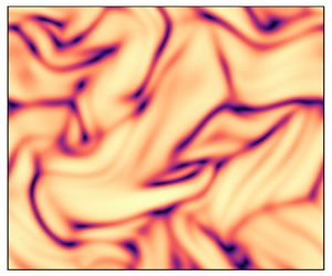
Figure 3(a) shows a snapshot of the scalar nematic order parameter $\mu$ for a simulation with $D_R = 0.01$ and $D_T = 10^{-3}$. The nematic order parameter consists of broad regions of high order $\mu \approx 0.5$, with narrow defect regions of low order $\mu \approx 0$. Figure 3(b) shows the spatiotemporal average of the nematic order parameter $\overline {\langle \mu \rangle _\varOmega } = (1/|\varOmega |)\overline {\int _\varOmega \mu \,{\rm d}\kern 0.06em \boldsymbol {x}}$ for simulations with various values of $D_R$ and $D_T$ compared with the theoretical bound $\mu ^*$ as defined by (4.13)–(4.14). The average increases with decreasing $D_R$ in agreement with the upper bound. Smaller values of the spatial diffusion coefficient tend to achieve values closer to the bound, though the bound still does not appear to be sharp in the unsteady regime as $D_T\rightarrow 0$.

Figure 3. (a) Scalar nematic order parameter $\mu$ for a simulation with $D_R = 0.01$ and $D_T = 10^{-3}$. (b) Time-averaged value $\overline {\langle \mu \rangle _\varOmega } =\overline {(\int _\varOmega \mu \,{\rm d}\kern 0.06em \boldsymbol {x})/|\varOmega |}$ compared with the theoretical bound $\mu ^*$ (solid line) for several values of $D_R$ and $D_T$. The bound holds across all parameter values tested, and is sharp past the nonlinear stability threshold (dashed line).

5. Discussion

This work provides analytical insight into the nonlinear dynamics of active nematic suspensions. Drawing on analogies with turbulent flows, the entropy method allowed us to derive rigorous bounds on the relative entropy and its fluctuations, establish a criterion for nonlinear stability, and bound time averages of orientational order parameters with relative ease. Moreover, this analysis holds independent of the boundary geometry under the provided boundary conditions. A key component of our analysis was the use of the Bingham distribution, whose properties made it possible to derive analytically tractable bounds on the rate of dissipation. All of these results extend naturally to three dimensions with slightly modified constants, though the optimal constant in the variational bound on rotational dissipation in § 3.3 requires more detailed calculation.

The behaviour of both simulations and the theoretical bound is remarkably similar to observations of bacterial turbulence in which orientation correlations and related order parameters increase with the volume fraction (Peng et al. Reference Peng, Liu and Cheng2021). This increase happens rapidly at a critical volume fraction $\phi \approx 0.01$, indicating a transition to instability, which is within the range of applicability of the dilute theory considered here (Doi & Edwards Reference Doi and Edwards1986). Under our non-dimensionalisation, the volume fraction is inversely proportional to $D_R$ so that the increasing bound as $D_R\rightarrow 0$ is both consistent with and suggestive of these observations. Detailed measurements of the diffusion coefficients would be useful to further corroborate these analytical predictions.

The entropy method is flexible and can be applied to other continuum models of active suspensions such as those that involve steric interactions (Ezhilan, Shelley & Saintillan Reference Ezhilan, Shelley and Saintillan2013; Gao & Li Reference Gao and Li2017), run and tumble dynamics (Subramanian & Koch Reference Subramanian and Koch2009) or chemotaxis (Lushi, Goldstein & Shelley Reference Lushi, Goldstein and Shelley2012). In these models other steady states may exist, in which case the relative entropy must be measured as a departure from another steady, possibly inhomogeneous, state $\tilde{\varPsi} = \tilde{\varPsi} ( \boldsymbol {x}, \boldsymbol {p})$,

(5.1)\begin{equation} \tilde{\mathcal{H}}(t) = \int_\varOmega \int_S \varPsi \log\left(\frac{\varPsi}{\tilde{\varPsi}}\right) {\rm d} \boldsymbol{p} \,{\rm d} \kern 0.06em \boldsymbol{x}. \end{equation}

This form of the relative entropy is also non-negative and vanishes only when $\varPsi = \tilde{\varPsi}$, however its rate of change involves additional terms that may include boundary contributions. The evolution of $\tilde {\mathcal {H}}$ may also depend on higher-order orientational moments of the distribution function, which could modify the constant in the logarithmic Sobolev inequality for minimisers of dissipation.

Motile suspensions in confinement are particularly interesting, since the isotropic state is not a valid solution as it violates the no-flux boundary condition $\partial \varPsi /\partial n = (\beta /D_T)(\kern 1.5pt \boldsymbol {p}\boldsymbol {\cdot }\hat {\boldsymbol {n}})\varPsi$, where $\beta$ is the swimming speed (Ezhilan & Saintillan Reference Ezhilan and Saintillan2015). Moreover, details of the particle geometry may need to be considered to account for admissible configurations near the boundary (Nitsche & Brenner Reference Nitsche and Brenner1990; Schiek & Shaqfeh Reference Schiek and Shaqfeh1995; Chen & Thiffeault Reference Chen and Thiffeault2021). Here the steady-state solution will depend on both the boundary geometry and the ratio of motility to spatial diffusion $\beta /D_T$, though the solution lacks a precise analytical form even in simple geometries. Such solutions, as well as their unsteady counterparts, are characterised by concentration boundary layers (Rothschild Reference Rothschild1963; Berke et al. Reference Berke, Turner, Berg and Lauga2008; Elgeti & Gompper Reference Elgeti and Gompper2013).

We emphasise the results here are limited to immotile suspensions, though numerical and experimental work has found motility has a weak effect on turbulent statistics (Stenhammar et al. Reference Stenhammar, Nardini, Nash, Marenduzzo and Morozov2017; Peng et al. Reference Peng, Liu and Cheng2021). The central challenge posed by particle motility is the lack of a maximum principle on concentration fluctuations from which the estimate (3.17) can be shown to have no upper bound. Nonetheless, numerical evidence suggests motile suspensions are stable at a threshold near that derived here, and further work should see whether the methods can be extended to determine more general bounds.

Acknowledgements

We thank G. Francfort and D. Stein for useful discussions, and thank M. Shelley for encouraging the publication of this work.

Declaration of interests

The author report no conflict of interest.

Appendix A. Improved constants for $2{\rm \pi} /n$-periodic functions

Suppose $f(\theta )$ is $2{\rm \pi} /n$-periodic, that is $f(\theta +2{\rm \pi} /n) = f(\theta )$, and define $g = f(\theta /n)$. Assume also that $\int _0^{2{\rm \pi} } f \,{\rm d} \theta = 1$. Making the change of variables $\theta ' = \theta /n$, we find

(A1)\begin{equation} \int_0^{2{\rm \pi}} g(\theta) \,{\rm d}\theta = \int_0^{2{\rm \pi}} f(\theta/n) \,{\rm d}\theta = n\int_0^{2{\rm \pi}/n} f(\theta') \,{\rm d}\theta'=1, \end{equation}

where we used the fact $f(\theta +2{\rm \pi} /n) = f(\theta )$. Define $\mathcal {H}[f] = \int _0^{2{\rm \pi} } f\log (2{\rm \pi} f) \,{\rm d} \theta$ and $\mathcal {I}[f] = \int _0^{2{\rm \pi} } |\partial _\theta f^{1/2}|^2 \,{\rm d} \theta$. Similar to before, we have

(A2)\begin{equation} \mathcal{H}[g] = \int_0^{2{\rm \pi}} g(\theta)\log(2{\rm \pi} g(\theta)) \,{\rm d}\theta = n \int_0^{2{\rm \pi}/n} f(\theta')\log(2{\rm \pi} f(\theta')) \,{\rm d}\theta' = \mathcal{H}[f]. \end{equation}

Applying the logarithmic Sobolev inequality to $g$ with the constant $C = 2$ gives

(A3)\begin{equation} \mathcal{H}[g] \leq 2\mathcal{I}[g]. \end{equation}

Evaluating $\mathcal {I}[g]$, we find

(A4)\begin{align} \mathcal{I}[g] &= \int_0^{2{\rm \pi}} |\partial_\theta g^{1/2}(\theta)|^2 \,{\rm d}\theta \nonumber\\ &= \frac{1}{n}\int_0^{2{\rm \pi}/n} |\partial_{\theta'} f^{1/2}(\theta')|^2 \,{\rm d}\theta' \nonumber\\ &= \frac{1}{n^2}\mathcal{I}[f]. \end{align}

We therefore have the inequality

(A5)\begin{equation} \mathcal{H}[f] \leq \frac{2}{n^2}\mathcal{I}[f]. \end{equation}

This inequality is optimal by considering the function $f_n = (1 + \varepsilon \cos n\theta )/2{\rm \pi}$ as $\varepsilon \rightarrow 0$.

Appendix B. Convexity and monotonicity of $\eta$

Let $\varPsi _B = \exp (\zeta + \xi \cos 2\theta )$ be the Bingham distribution and consider its relative entropy density $\eta = (\zeta -\zeta _0) + 2\mu \xi$, where $\zeta = -\log (2{\rm \pi} I_0(\xi ))$. Differentiating with respect to $\mu$ gives

(B1)\begin{equation} \frac{{\rm d}\eta}{{\rm d}\mu} = \frac{{\rm d}\zeta}{{\rm d}\mu} + 2\xi + 2\mu\frac{{\rm d}\xi}{{\rm d}\mu} = 2\xi \end{equation}

and

(B2)\begin{equation} \frac{{\rm d}^2\eta}{{\rm d}\mu^2} = 2\frac{{\rm d}\xi}{{\rm d}\mu}, \end{equation}

where we used $\zeta ' = -2\mu \xi '$. Since $\xi \geq 0$, we have ${\rm d} \eta /{\rm d} \mu \geq 0$ and so $\eta$ is a monotonic function of $\mu$. Using the identity $\mu = I_1(\xi )/2I_0(\xi )$, we find

(B3)\begin{equation} 2 = \left[\frac{1}{2} + \frac{1}{2}\frac{I_2(\xi)}{I_0(\xi)} - \left(\frac{I_1(\xi)}{I_0(\xi)}\right)^2\right]\frac{{\rm d}\xi}{{\rm d}\mu},\end{equation}

where we have also used $I_1'(\xi ) = (I_2(\xi ) + I_0(\xi ))/2$. It is sufficient to show the bracketed term in (B3) is positive from which we can conclude ${\rm d} \xi /{\rm d} \mu > 0$ and, hence, ${\rm d} ^2\eta /{\rm d} \mu ^2 > 0$, implying $\eta$ is convex. Now define $S = Z^{-1}\int _0^{2{\rm \pi} } \cos ^4\theta \exp ({\xi \cos 2\theta })\,{\rm d} \theta$ to be the fourth moment of the Bingham distribution. In terms of $\xi$, this can be written as

(B4)\begin{equation} S = \frac{1}{8}\left(3 + 4\frac{I_1(\xi)}{I_0(\xi)} + \frac{I_2(\xi)}{I_0(\xi)}\right). \end{equation}

Using this to solve for $I_2(\xi )/I_0(\xi )$, we find

(B5)\begin{align} \frac{1}{2} + \frac{1}{2}\frac{I_2(\xi)}{I_0(\xi)} - \left(\frac{I_1(\xi)}{I_0(\xi)}\right)^2 &={-}1 - 4\mu + 4S - 4\mu^2 \nonumber\\ &= 4S - 4(\mu + 1/2)^2 \nonumber\\ &= 4(S - m^2), \end{align}

where $m = Z^{-1} \int _0^{2{\rm \pi} } \cos ^2\theta \exp ({\xi \cos 2\theta })$ is the second moment of the Bingham distribution. The variance inequality ${\langle\, f\rangle ^2 \leq \langle\, f^2\rangle }$ with $f = \cos ^2\theta$ implies $m^2 \leq S$, so the claim holds.

References

Albritton, D. & Ohm, L. 2023 On the stabilizing effect of swimming in an active suspension. SIAM J. Math. Anal. 55 (6), 60936132.10.1137/22M1496037CrossRefGoogle Scholar
Alert, R., Casademunt, J. & Joanny, J.-F. 2022 Active turbulence. Annu. Rev. Condens. Matter Phys. 13 (1), 143170.10.1146/annurev-conmatphys-082321-035957CrossRefGoogle Scholar
Arfken, G.B., Weber, H.J. & Harris, F.E. 2011 Mathematical Methods for Physicists: A Comprehensive Guide. Academic.Google Scholar
Arnold, A., Carrillo, J.A., Desvillettes, L., Dolbeault, J., Jüngel, A., Lederman, C., Markowich, P.A., Toscani, G. & Villani, C. 2004 Entropies and equilibria of many-particle systems: an essay on recent research. In Nonlinear Differential Equation Models, pp. 35–43. Springer.10.1007/978-3-7091-0609-9_5CrossRefGoogle Scholar
Berke, A.P., Turner, L., Berg, H.C. & Lauga, E. 2008 Hydrodynamic attraction of swimming microorganisms by surfaces. Phys. Rev. Lett. 101, 038102.10.1103/PhysRevLett.101.038102CrossRefGoogle ScholarPubMed
Brigati, G., Dolbeault, J. & Simonov, N. 2022 Logarithmic Sobolev and interpolation inequalities on the sphere: constructive stability results. arXiv:2211.13180.10.4171/aihpc/106CrossRefGoogle Scholar
Chaubal, C.V. & Leal, L.G. 1998 A closure approximation for liquid-crystalline polymer models based on parametric density estimation. J. Rheol. 42 (1), 177201.10.1122/1.550887CrossRefGoogle Scholar
Chen, H. & Thiffeault, J.-L. 2021 Shape matters: a Brownian microswimmer in a channel. J. Fluid Mech. 916, A15.10.1017/jfm.2021.144CrossRefGoogle Scholar
Chen, X. & Liu, J.-G. 2013 Global weak entropy solution to Doi–Saintillan–Shelley model for active and passive rod-like and ellipsoidal particle suspensions. J. Differ. Equ. 254 (7), 27642802.10.1016/j.jde.2013.01.005CrossRefGoogle Scholar
Constantin, P. 2005 Nonlinear Fokker–Planck Navier–Stokes systems. Commun. Math. Sci. 3 (4), 531544.10.4310/CMS.2005.v3.n4.a4CrossRefGoogle Scholar
Constantin, P. & Masmoudi, N. 2008 Global well-posedness for a Smoluchowski equation coupled with Navier–Stokes equations in 2D. Commun. Math. Phys. 278 (1), 179191.10.1007/s00220-007-0384-2CrossRefGoogle Scholar
Coti Zelati, M., Dietert, H. & Gérard-Varet, D. 2023 Orientation mixing in active suspensions. Ann. PDE 9 (2), 20.10.1007/s40818-023-00163-8CrossRefGoogle Scholar
Cover, T.M. & Thomas, J.A. 2012 Elements of Information Theory. Wiley.Google Scholar
Doering, C.R. & Constantin, P. 1992 Energy dissipation in shear driven turbulence. Phys. Rev. Lett. 69, 16481651.10.1103/PhysRevLett.69.1648CrossRefGoogle ScholarPubMed
Doering, C.R. & Gibbon, J.D. 1995 Applied Analysis of the Navier–Stokes Equations, Cambridge Texts in Applied Mathematics, vol. 2. Cambridge University Press.10.1017/CBO9780511608803CrossRefGoogle Scholar
Doi, M. & Edwards, S.F. 1986 The Theory of Polymer Dynamics. Oxford University Press.Google Scholar
Dolbeault, J. & Toscani, G. 2016 Stability results for logarithmic Sobolev and Gagliardo–Nirenberg inequalities. Intl Math. Res. Not. 2016 (2), 473498.Google Scholar
Dombrowski, C., Cisneros, L., Chatkaew, S., Goldstein, R.E. & Kessler, J.O. 2004 Self-concentration and large-scale coherence in bacterial dynamics. Phys. Rev. Lett. 93, 098103.10.1103/PhysRevLett.93.098103CrossRefGoogle ScholarPubMed
Doostmohammadi, A., Ignés-Mullol, J., Yeomans, J.M. & Sagués, F. 2018 Active nematics. Nat. Commun. 9 (1), 3246.10.1038/s41467-018-05666-8CrossRefGoogle ScholarPubMed
Dunkel, J., Heidenreich, S., Drescher, K., Wensink, H.H., Bär, M. & Goldstein, R.E. 2013 Fluid dynamics of bacterial turbulence. Phys. Rev. Lett. 110, 228102.10.1103/PhysRevLett.110.228102CrossRefGoogle ScholarPubMed
Elgeti, J. & Gompper, G. 2013 Wall accumulation of self-propelled spheres. Europhys. Lett. 101 (4), 48003.10.1209/0295-5075/101/48003CrossRefGoogle Scholar
Evans, L.C. 2010 Partial Differential Equations, Graduate Studies in Mathematics. American Mathematical Society.10.1090/gsm/019CrossRefGoogle Scholar
Ezhilan, B. & Saintillan, D. 2015 Transport of a dilute active suspension in pressure-driven channel flow. J. Fluid Mech. 777, 482522.10.1017/jfm.2015.372CrossRefGoogle Scholar
Ezhilan, B., Shelley, M.J. & Saintillan, D. 2013 Instabilities and nonlinear dynamics of concentrated active suspensions. Phys. Fluids 25 (7), 070607.10.1063/1.4812822CrossRefGoogle Scholar
Fantuzzi, G., Arslan, A. & Wynn, A. 2022 The background method: theory and computations. Phil. Trans. R. Soc. A 380 (2225), 20210038.10.1098/rsta.2021.0038CrossRefGoogle ScholarPubMed
Freund, J.B. 2023 Object transport by a confined active suspension. J. Fluid Mech. 960, A16.10.1017/jfm.2023.191CrossRefGoogle Scholar
Gao, T., Betterton, M.D., Jhang, A.-S. & Shelley, M.J. 2017 Analytical structure, dynamics, and coarse graining of a kinetic model of an active fluid. Phys. Rev. Fluids 2, 093302.10.1103/PhysRevFluids.2.093302CrossRefGoogle Scholar
Gao, T. & Li, Z. 2017 Self-driven droplet powered by active nematics. Phys. Rev. Lett. 119, 108002.10.1103/PhysRevLett.119.108002CrossRefGoogle ScholarPubMed
Gross, L. 1975 Logarithmic Sobolev inequalities. Am. J. Math. 97 (4), 10611083.10.2307/2373688CrossRefGoogle Scholar
Hohenegger, C. & Shelley, M.J. 2010 Stability of active suspensions. Phys. Rev. E 81, 046311.10.1103/PhysRevE.81.046311CrossRefGoogle ScholarPubMed
Ifantis, E.K. & Siafarikas, P.D. 1990 Inequalities involving Bessel and modified Bessel functions. J. Math. Anal. Appl. 147 (1), 214227.10.1016/0022-247X(90)90394-UCrossRefGoogle Scholar
Li, S., Wang, W. & Zhang, P. 2015 Local well-posedness and small Deborah limit of a molecule-based $Q$-tensor system. Discr. Contin. Dyn. Syst. B 20 (1531), 2611.10.3934/dcdsb.2015.20.2611CrossRefGoogle Scholar
Liu, Z., Zeng, W., Ma, X. & Cheng, X. 2021 Density fluctuations and energy spectra of 3D bacterial suspensions. Soft Matt. 17, 1080610817.10.1039/D1SM01183ACrossRefGoogle ScholarPubMed
Lushi, E., Goldstein, R.E. & Shelley, M.J. 2012 Collective chemotactic dynamics in the presence of self-generated fluid flows. Phys. Rev. E 86, 040902.10.1103/PhysRevE.86.040902CrossRefGoogle ScholarPubMed
Majda, A.J. & Bertozzi, A.L. 2001 Vorticity and Incompressible Flow, Cambridge Texts in Applied Mathematics. Cambridge University Press.10.1017/CBO9780511613203CrossRefGoogle Scholar
Narayan, V., Ramaswamy, S. & Menon, N. 2007 Long-lived giant number fluctuations in a swarming granular nematic. Science 317 (5834), 105108.10.1126/science.1140414CrossRefGoogle Scholar
Nitsche, J.M. & Brenner, H. 1990 On the formulation of boundary conditions for rigid nonspherical Brownian particles near solid walls: applications to orientation-specific reactions with immobilized enzymes. J. Colloid Interface Sci. 138 (1), 2141.10.1016/0021-9797(90)90177-PCrossRefGoogle Scholar
Ohm, L. & Shelley, M.J. 2022 Weakly nonlinear analysis of pattern formation in active suspensions. J. Fluid Mech. 942, A53.10.1017/jfm.2022.392CrossRefGoogle Scholar
Peng, Y., Liu, Z. & Cheng, X. 2021 Imaging the emergence of bacterial turbulence: phase diagram and transition kinetics. Sci. Adv. 7 (17), eabd1240.10.1126/sciadv.abd1240CrossRefGoogle ScholarPubMed
Rothschild, L. 1963 Non-random distribution of bull spermatozoa in a drop of sperm suspension. Nature 198 (4886), 12211222.10.1038/1981221a0CrossRefGoogle Scholar
Saintillan, D. & Shelley, M.J. 2008 Instabilities and pattern formation in active particle suspensions: kinetic theory and continuum simulations. Phys. Rev. Lett. 100, 178103.10.1103/PhysRevLett.100.178103CrossRefGoogle ScholarPubMed
Saintillan, D. & Shelley, M.J. 2013 Active suspensions and their nonlinear models. C. R. Phys. 14 (6), 497–517.10.1016/j.crhy.2013.04.001CrossRefGoogle Scholar
Sanchez, T., Chen, D.T.N., DeCamp, S.J., Heymann, M. & Dogic, Z. 2012 Spontaneous motion in hierarchically assembled active matter. Nature 491, 431434.10.1038/nature11591CrossRefGoogle ScholarPubMed
Schiek, R.L. & Shaqfeh, E.S.G. 1995 A nonlocal theory for stress in bound, Brownian suspensions of slender, rigid fibres. J. Fluid Mech. 296, 271324.10.1017/S0022112095002138CrossRefGoogle Scholar
Simha, R.A. & Ramaswamy, S. 2002 Statistical hydrodynamics of ordered suspensions of self-propelled particles: waves, giant number fluctuations and instabilities. Physica A 306, 262269.10.1016/S0378-4371(02)00503-4CrossRefGoogle Scholar
Škultéty, V., Nardini, C., Stenhammar, J., Marenduzzo, D. & Morozov, A. 2020 Swimming suppresses correlations in dilute suspensions of pusher microorganisms. Phys. Rev. X 10, 031059.Google Scholar
Stenhammar, J., Nardini, C., Nash, R.W., Marenduzzo, D. & Morozov, A. 2017 Role of correlations in the collective behavior of microswimmer suspensions. Phys. Rev. Lett. 119, 028005.10.1103/PhysRevLett.119.028005CrossRefGoogle ScholarPubMed
Straughan, B. 1992 The Energy Method, Stability, and Nonlinear Convection, Applied Mathematical Sciences, vol. 2. Springer.10.1007/978-1-4757-2194-2CrossRefGoogle Scholar
Subramanian, G. & Koch, D.L. 2009 Critical bacterial concentration for the onset of collective swimming. J. Fluid Mech. 632, 359400.10.1017/S002211200900706XCrossRefGoogle Scholar
Thiffeault, J.-L. 2021 Nonuniform mixing. Phys. Rev. Fluids 6, 090501.10.1103/PhysRevFluids.6.090501CrossRefGoogle Scholar
Weady, S., Shelley, M.J. & Stein, D.B. 2022 a A fast Chebyshev method for the Bingham closure with application to active nematic suspensions. J. Comput. Phys. 457, 110937.10.1016/j.jcp.2021.110937CrossRefGoogle Scholar
Weady, S., Stein, D.B. & Shelley, M.J. 2022 b Thermodynamically consistent coarse-graining of polar active fluids. Phys. Rev. Fluids 7, 063301.10.1103/PhysRevFluids.7.063301CrossRefGoogle Scholar
Wensink, H.H., Dunkel, J., Heidenreich, S., Drescher, K., Goldstein, R.E., Löwen, H. & Yeomans, J.M. 2012 Meso-scale turbulence in living fluids. Proc. Natl Acad. Sci. USA 109 (36), 1430814313.10.1073/pnas.1202032109CrossRefGoogle ScholarPubMed
Figure 0

Figure 1. Minimising distribution $\varPsi _\mu$ of rotational dissipation subject to constraints on the largest eigenvalue $\mu$ of $\boldsymbol{\mathsf{D}}/c$. The distribution is bimodal with peaks whose amplitudes increase monotonically with $\mu$.

Figure 1

Figure 2. Bounds on the relative entropy of the Bingham distribution. The solid line shows the time-averaged bound $\eta ^*(D_R)$ and the dot-dashed line shows the spatially averaged uniform-in-time bound. Beyond the nonlinear stability threshold $D_R > 1/16$ (dashed line), the bound is zero, consistent with nonlinear stability. As $D_R\rightarrow 0$, the bound diverges.

Figure 2

Figure 3. (a) Scalar nematic order parameter $\mu$ for a simulation with $D_R = 0.01$ and $D_T = 10^{-3}$. (b) Time-averaged value $\overline {\langle \mu \rangle _\varOmega } =\overline {(\int _\varOmega \mu \,{\rm d}\kern 0.06em \boldsymbol {x})/|\varOmega |}$ compared with the theoretical bound $\mu ^*$ (solid line) for several values of $D_R$ and $D_T$. The bound holds across all parameter values tested, and is sharp past the nonlinear stability threshold (dashed line).