Hostname: page-component-586b7cd67f-l7hp2 Total loading time: 0 Render date: 2024-11-27T02:52:41.801Z Has data issue: false hasContentIssue false

A unified theoretical model for spatiotemporal development of Rayleigh–Taylor and Richtmyer–Meshkov fingers

Published online by Cambridge University Press:  29 December 2022

Changwen Liu
Affiliation:
HEDPS, Center for Applied Physics and Technology, College of Engineering, Peking University, Beijing 100871, PR China State Key Laboratory for Turbulence and Complex Systems, College of Engineering, Peking University, Beijing 100871, PR China
Yousheng Zhang*
Affiliation:
HEDPS, Center for Applied Physics and Technology, College of Engineering, Peking University, Beijing 100871, PR China Institute of Applied Physics and Computational Mathematics, Beijing 100094, PR China
Zuoli Xiao*
Affiliation:
HEDPS, Center for Applied Physics and Technology, College of Engineering, Peking University, Beijing 100871, PR China State Key Laboratory for Turbulence and Complex Systems, College of Engineering, Peking University, Beijing 100871, PR China Nanchang Innovation Institute, Peking University, Nanchang 330008, PR China
*
Email addresses for correspondence: [email protected], [email protected]

Abstract

An initially perturbed interface between two fluids of different densities is usually unstable when driven by an acceleration or a shock wave; it is known as a Rayleigh–Taylor instability or a Richtmyer–Meshkov instability. One of the most significant issues in these instabilities is the spatiotemporal development of fingers generated at the interface, which plays an important role in both scientific research (e.g. supernova explosion) and engineering applications (e.g. inertial confinement fusion). Accurate theoretical solution of these interfacial fingers remains as an unsolved and challenging problem since Taylor's seminal work more than seven decades ago. This paper reports a unified theory established for such phenomena by combining the classical potential-flow theory and a dual-source model to address the long-standing difficulty highlighted by the initial-value sensitivity and strong nonlinearity. It is the first time for a theory to accurately predict the long-time developments in both growth rate and shape curvature of interfacial fingers at all density ratios in two and three dimensions. Moreover, the new theory clearly reveals the nonlinear coupling mechanism for interfacial evolution, and especially explains the origin of overshot in the growth rate curve.

Type
JFM Papers
Copyright
© The Author(s), 2022. Published by Cambridge University Press

1. Introduction

The initially perturbed interface of two fluids is usually unstable when driven by an acceleration ${g}$ pointing from a heavy fluid to a light one or impinged by a shock wave; they are known as a Rayleigh–Taylor instability (RTI) (Rayleigh Reference Rayleigh1883; Taylor Reference Taylor1950) and a Richtmyer–Meshkov instability (RMI) (Richtmyer Reference Richtmyer1960; Meshkov Reference Meshkov1969), respectively. With the development of such hydrodynamic instabilities, light and heavy fluids penetrate into each other, resulting in the formation of bubble- and spike-like finger structures (Zhou Reference Zhou2017a,Reference Zhoub). These phenomena play important roles in both scientific research and engineering applications, such as supernova explosions (see, e.g. Adam Reference Adam2000; Isobe et al. Reference Isobe, Miyagoshi, Shibata and Yokoyama2005; Cabot & Cook Reference Cabot and Cook2006; Uchiyama et al. Reference Uchiyama, Aharonian, Tanaka, Takahashi and Maeda2007) and inertial confinement fusion (see, e.g. Clery Reference Clery2015; Betti & Hurricane Reference Betti and Hurricane2016; Casey et al. Reference Casey2017; Ding et al. Reference Ding, Si, Yang, Lu, Zhai and Luo2017; Matsuo et al. Reference Matsuo, Sano, Nagatomo, Somekawa, Law, Morita, Arikawa and Fujioka2021; Sabet et al. Reference Sabet, Hassanzadeh, De Wit and Abedi2021). Two recent survey studies provide a systematic review on RTI and RMI phenomena, which make the corresponding applications accessible to a broad and varied audience (Zhou et al. Reference Zhou, Clark, Clark, Gail Glendinning, Aaron Skinner, Huntington, Hurricane, Dimits and Remington2019, Reference Zhou2021). An important issue of these classical hydrodynamic instabilities is how these finger structures on an unstable interface grow in time and space. There have been sets of experimental (Jacobs & Catton Reference Jacobs and Catton1988; Luo, Wang & Si Reference Luo, Wang and Si2013; Liu et al. Reference Liu, Liang, Ding, Liu and Luo2018; Luo et al. Reference Luo, Zhang, Ding, Si, Yang, Zhai and Wen2018; Liang et al. Reference Liang, Zhai, Ding and Luo2019; Lherm et al. Reference Lherm, Deguen, Alboussière and Landeau2022) and numerical (Ristorcelli & Clark Reference Ristorcelli and Clark2004; Ramaprabhu, Dimonte & Andrews Reference Ramaprabhu, Dimonte and Andrews2005; Li et al. Reference Li, Fu, Yu and Li2021; Yan et al. Reference Yan, Fu, Wang, Yu and Li2022) data available for their growth rate and shape evolution since Taylor's pioneering work in 1950, and yet there is still a lack of a unified and accurate theory to characterize them.

The classical work of Rayleigh (Reference Rayleigh1883) on hydrodynamic instability, along with its modern development by Taylor (Reference Taylor1950), has been expanded by several milestone-like theories based on Layzer's potential-flow model (LPM) (see, e.g. Layzer Reference Layzer1955; Hecht, Alon & Shvarts Reference Hecht, Alon and Shvarts1994; Alon et al. Reference Alon, Hecht, Ofer and Shvarts1995; Qiang & Sohn Reference Qiang and Sohn1996; Mikaelian Reference Mikaelian1998; Zhang Reference Zhang1998; Goncharov Reference Goncharov2002; Abarzhi, Glimm & Lin Reference Abarzhi, Glimm and Lin2003; Mikaelian Reference Mikaelian2003; Sohn Reference Sohn2003; Zhang & Guo Reference Zhang and Guo2016; Zhang, Deng & Guo Reference Zhang, Deng and Guo2018; Guo & Zhang Reference Guo and Zhang2020; Zhao et al. Reference Zhao, Wang, Liu and Lu2020). These studies show that the interface evolution of single-mode RTI usually undergoes a linear stage, a nonlinear stage, quasisteady stages with constant growth rate, and other possible stages. Specifically, Mikaelian (Reference Mikaelian1998) and Zhang (Reference Zhang1998) are among the first to give the evolutions of bubble and spike, respectively, in a fluid–vacuum configuration. It is Goncharov (Reference Goncharov2002) who generalizes this method to an arbitrary density ratio. Recently, Zhang & Guo (Reference Zhang and Guo2016) and Guo & Zhang (Reference Guo and Zhang2020) obtained a universal finger evolution for arbitrary density ratio and Zhao et al. (Reference Zhao, Wang, Liu and Lu2020) further applied it to RTI in a cylindrical geometry.

In the framework of original LPM, the sinusoidal potential function is employed to describe the flow of the fingertip and its immediate neighbourhood, which only approximately satisfies the dynamic condition of constant surface pressure. Meanwhile, most of these theories usually assume that the shape of the fingertip does not change with time in prediction of the growth rate, which is in conflict with numerical simulations from Sohn (Reference Sohn2004) and Ramaprabhu & Dimonte (Reference Ramaprabhu and Dimonte2005) and causes unphysical predictions in growth rate (Krechetnikov Reference Krechetnikov2009). According to Kull (Reference Kull1983), the correctness of such potential functions without harmonics and possible singularities is questionable or hard to justify theoretically. In addition, it is found that the gravitational acceleration obtained based on the sinusoidal potential model increases rapidly below the fingertip and the increase trend becomes stronger for larger initial amplitudes (Kull Reference Kull1986). This indicates that the acceleration in the flow field given by the sinusoidal potential flow model is non-uniform, which is obviously different from the fact that the acceleration, as a conservative force, should be uniform in the whole flow field. Since the growth rate depends weakly on the acceleration non-uniformities, the original LPM proves rather successful in describing the growth rate compared with the result from numerical simulation. However, the original LPM fails to capture the curvature of the fingertip accurately, which is a more sensitive parameter and is found to be only approximately ${2/3}$ of the value obtained numerically at the quasisteady stage (Kull Reference Kull1986). Different from others, Zufiria (Reference Zufiria1988) allows time dependence of the shape based on a single-point source model introduced by Kull (Reference Kull1986), which can lead to a better approximation for shape, but only for a vacuum–bubble configuration. Sohn & Zhang (Reference Sohn and Zhang2001) also make use of such an assumption in comparison with the original LPM in a fluid–vacuum configuration. Nevertheless, no further results are secured due to mathematical complexity. Therefore, there still lacks a well-unified theory that can simultaneously predict the growth rate and shape evolution from early to late stages and is suitable for all density ratios, which motivates the present work.

This paper is intended to develop a new theory to address the long-standing problem within the LPM framework. The present theory is established qualitatively by introducing a dual-source model to mimic the pattern of real flow, and is further formulated quantitatively with the constraint of the geometric similarity principle. The derived equations can simultaneously predict the growth rate and shape evolution. It should be stressed that the new theory focuses on the development of instability up to the quasisteady stage similar to most of previous studies. The results are in good agreement with numerical and experimental data in both RTI and RMI regimes at all density ratios in different dimensions. Moreover, the theoretical model can help reveal the underlying nonlinear coupling mechanism between growth rate and shape evolution, and explain the origin of the overshot phenomenon in variation of the perturbation growth rate.

The remaining paper is structured as follows. First, theoretical analysis and derivations are given in § 2. Then, the dual-source model is validated for both RTI and RMI flow regimes in § 3. Finally, conclusion and discussion are made in § 4. For completeness, the detailed formulations for the present new theory are provided as Appendix A.

2. Theoretical analysis and formulations

For the purpose of clarity in subsequent discussions, we begin with an introduction of the LPM. In the two-dimensional (2-D) case, we consider two incompressible inviscid fluids in a vertically infinite strip with its left and right boundaries satisfying a no-penetration condition. The initial interface is characterized by a single-mode sinusoidal perturbation. The LPM for RTI problem can be described by the following governing equations (Goncharov Reference Goncharov2002):

(2.1)\begin{gather} {\nabla ^2}\varphi _{i} = 0, \end{gather}
(2.2)\begin{gather}\dot{\eta} - \varphi _{i,x} \eta_x + \varphi _{i,z} = 0, \end{gather}
(2.3)\begin{gather}\sum_{i = 1}^2 {{{( - 1)}^i}} {\rho _i} \left[{-}g\eta + \dot{\varphi}_i -\frac{1}{2}({\varphi _{i,x}^2}+{\varphi _{i,z}^2})\right]=f(t). \end{gather}

Here $x$ and $z$ are the coordinates perpendicular and parallel to the acceleration ${g}$, respectively. Subscripts ${i=1,2}$ denote the upstream and downstream fluids, respectively. Here ${\varphi _{i}}$ is the velocity potential function, and ${f(t)}$ only depends on time $t$. According to the LPM, the shape of the fingertip is approximated as a parabola of the form ${\eta ( x,t )=z_0(t) + \xi (t)x^2}$, where ${z_0(t)}$ and ${\xi (t)}$ are the vertical position and curvature of the finger, which are used to characterize the growth rate and shape evolution, respectively. It is worth stressing that the traditional LPM only considers behaviour of the single finger located in the middle of the channel, and assumes that the fingers near the two sides of the strip have no dynamic effect on the middle one, as shown in figure 1(a). Furthermore, the LPM only describes the flow in the neighbourhood of the interface fingertip instead of the whole interface because the vorticity generated in the flow field may invalidate the potential function hypothesis far away from the fingertip. In three-dimensional (3-D) geometry, the above process can be easily extended to a cylindrical coordinate system with the $z$ axis in the direction of density gradient and the $x$ axis interpreted as the radial coordinate by assuming cylindrical symmetry of the fingers.

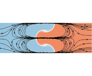
Figure 1. (a) Schematics of the dual-source model. The finger is generated by the penetration of downstream fluid ${(\rho _{1})}$ into the upstream fluid ${(\rho _{2})}$. Two sources are separated by the finger with each being located at a distance ${a_{i}(t)}$ from the fingertip with an intensity ${Q_{i}(t)}$. Here ${\lambda _{i}}$ is the characteristic wavelength of the potential function ${\varphi _{i}}$. The red solid parabola is the middle finger approximated by LPM and the blue dashed parabolas are fingers neglected in LPM. The dashed lines with arrows are streamlines induced by the present model. (b) Streamlines of the flow field obtained from the present numerical simulation of RTI ($A=0.15$), which are overlaid on contours of densities.

For the LPM, the key to accurately solving the interfacial fingers is to construct a reasonable velocity potential function ${\varphi _{i}}$. As for the treatment in the original LPM, the simplest sinusoidal potential function ${\varphi _{i}=\sum _{n} a_{i}^{n}(t)\cos (nkx)\exp ({(-1)^{i}nkz})}$ is introduced to describe the flow immediately around the fingertip with the constraint of approximately constant surface pressure. This form of ${\varphi _{i}}$ proves to capture the evolution of finger growth rate well, but the predicted curvature can deviate strongly from the numerical result (especially at the quasisteady stage), which is ascribed to the violation of uniform acceleration. Although efforts have been taken to improve the prediction ability for uniform acceleration and finger curvature by introducing source(s) (Kull Reference Kull1986; Zufiria Reference Zufiria1988; Sohn & Zhang Reference Sohn and Zhang2001), few advances are made beyond the fluid–vacuum configuration. Therefore, suitable potential functions ${\varphi _{i}}$ for all density ratios are expected to describe the development of the interface finger.

Previous experiments and numerical simulations show that the finger development is closely related to the initial conditions. Therefore, a good theory should consider and solve the issue of initial-value sensitivity. Furthermore, it is observed that the growth rate and shape evolution of fingers are coupled with each other, and their strong nonlinear interaction should also be taken into account. These two challenges may be the major obstacles to develop an accurate theory for classical hydrodynamic instabilities. As discussed above, however, no available theory satisfies these requirements to date. To this end, we develop a novel theory by including the evolution of the fingers’ shape. Through the physical image of RTI (see figure 1b), we are surprised that there are always dual-source singularities combined with a uniform stream on both sides of the finger. Both of them are generated at the initial time and only change the distance from the interface due to the temporal variation of source intensity. Thus, the streamlines in a flow field should always meet the condition of dual-source no matter how the initial perturbation changes. Moreover, the initial effect gradually decays with the further development of fingers, and the strong nonlinear coupling between growth rate and shape evolution begins to dominate. Although the finger undergoes a nonlinear development, the fingertip structure always maintains a self-similar pattern. With these understandings, our approach consists of two steps: (i) construct a dual-source field by simulating the initial flow pattern to satisfy the initial-value sensitivity; and (ii) maintain the dual-source characteristics to guarantee the self-similar evolution of the interface and further restrict the nonlinear interaction. Based on the assumption of LPM and the numerical flow field (figure 1b), the RTI flow field is simplified as that depicted in figure 1(a). It is assumed that the flow field near the finger is generated by two sources distributed on the upstream and downstream sides of the interface, respectively. Each source is located in a distance ${a_{i}(t)}$ from the fingertip with source intensity ${Q_{i}(t)}$. It should be stressed that the potential functions ${\varphi _{i}}$ must obey the following constraints: (i) being a solution of (2.1); (ii) satisfying the symmetric and far-field boundary conditions as sketched in figure 1(a); (iii) avoiding an imaginary component in the solution (Goncharov Reference Goncharov2002). By taking these constraints into consideration and referring to the research works by Zufiria (Reference Zufiria1988) and Sohn & Zhang (Reference Sohn and Zhang2001), a new potential function ${\varphi _{i}}$ for the 2-D case can be obtained in the form

(2.4)\begin{equation} \varphi _{i}= {\rm Real}\left\{ {{Q_i}(t)\ln {\frac{{\sinh [(z + jx + {a_i(t)}){k_i}/2]}}{{\exp [(z + jx + {a_i(t)}){k_i}/2]}}} } \right\}, \end{equation}

where ${j^2=-1}$, the hyperbolic part (${\sinh }$) represents the source flow and the exponential part ($\exp$) represents the uniform flow. For comparison purposes, the streamlines for the pure source flow (induced by the hyperbolic part) and combined flow (induced by dual-source singularities in combination with a uniform stream) are shown in figures 2(a) and 2(b), respectively. Here, the parameters are set to $Q_{i}=1$, $k_{i}=1$ and $a_{i}=2(-1)^{i}$ without loss of generalization. From figure 2(b), one can clearly see that the patterns of combined flow are quite similar to those observed for the simulated RTI flow both upstream and downstream of the interface as shown in figure 1(b). It needs to be mentioned that the flow patterns in figure 2(b) are only a qualitative display of the potential function (2.4), and the realistic flow field should be further constrained by (2.2). Nevertheless, it is shown that the potential function (2.4) can successfully reflect typical characteristics of the target flow field. Since there is no concise complex potential function for 3-D flow, the series forms of this new potential function ${\varphi _{i}}$ are employed to facilitate the unified solution, which reads

(2.5)\begin{gather} \varphi _{i}= Q_{i}(t)\sum_{n=0}^{\infty}\frac{\cos\left[(2n+1)k_{i}x\right]\exp({({-}1)^i(2n+1)k_{i}(z+a_{i}(t))})}{2n+1} , \end{gather}
(2.6)\begin{gather}\varphi _{i}= Q_{i}(t)\sum_{n=0}^{\infty}\frac{{\rm J}_0\left[(2n+1)k_{i}x\right]\exp({({-}1)^i(2n+1)k_{i}(z+a_{i}(t))})}{2n+1} , \end{gather}

where (2.5) and (2.6) are the expressions for the 2-D and 3-D cases, respectively. Here ${k_{i}\equiv 2{\rm \pi} /\lambda _{i}}$ is the wavenumber, and ${{\rm J}_{0}(x)}$ is the zero-order Bessel function. For a specific ${\varphi _{i}}$, one can readily obtain the flow field in the vicinity of the interface as illustrated by the streamlines (dashed lines) in figure 1(a). As can be seen, the streamlines are consistent with the current numerical simulation shown in figure 1(b), which implies the rationality of the present dual-source figure for ${\varphi _{i}}$. It should be mentioned that the present model readily recovers previous potential flow models (e.g. Zhang Reference Zhang1998; Goncharov Reference Goncharov2002; Zhang & Guo Reference Zhang and Guo2016) when the expansion order $n\leq 2$ and wavenumbers $k_1=k_2$. Meanwhile, the new velocity potential function ${\varphi _{i}}$ involves only two time-dependent unknown quantities ($Q_{i}(t),a_{i}(t)$) due to the dual-source constraint.

Figure 2. The streamlines for flow induced by (a) pure sources (i.e. the hyperbolic part in (2.4)) and (b) source-uniform flow combination (dual-source singularities combined with a uniform stream, i.e. both the hyperbolic and exponential parts in (2.4)).The parameters are taken as $Q_{i}=1$, $k_{i}=1$ and $a_{i}=2(-1)^{i}$ for reference.

As one can imagine from figure 1(a), the channel should not be completely occupied by the middle finger (approximated by a parabola) due to the existence of fingers near both channel walls (which are neglected in LPM). In the real physical picture, when the convex curve (the red solid parabola) and concave curve (the blue dashed parabola) intersects, there are always two points where the tangent line is parallel to the channel wall, and the non-penetrability condition of the interface is satisfied. The distance between these two points ${\lambda _{1}}$ represents the characteristic scale of the finger. Therefore, according to the parabolic approximation of LPM, the velocity potential function ${\varphi _{1}}$ should be characterized by ${\lambda _{1}}$ (corresponding to wavenumber ${k_{1}}$), while ${\varphi _{2}}$ should always reflect the scale of channel width ${\lambda _{2}}$ (corresponding to wavenumber ${k_{2}}$). For such a purpose, the potential function on each side of the finger does not have to share the domain. Note that the wavenumbers ${k_{1}}$ and ${k_{2}}$ in the potential functions are not employed to reflect the lateral scale of the whole interface, but to characterize the local fluid motion near the fingertip. In addition, the results from numerical simulations and experiments show that the evolution of fingers are self-similar. Qualitatively, it implies that the fluid between the source and fingertip approximately satisfies the geometric similarity, which leads to ${\lambda _{1}^{0}a_{1}^{0}=\lambda _{1}a_{1}}$, with the superscript ‘0’ representing the initial time. Based on this assumption, one ends up with the following relation for the ratio of wavenumbers:

(2.7)\begin{equation} c\left( {A,t} \right) \equiv \frac{{{\lambda _1}}}{{{\lambda _2}}} = \frac{{{k_2}}}{{{k_1}}} = \frac{{\lambda _1^0}}{{{\lambda _2}}}\frac{{a_1^0}}{{{a_1}}} = {c^0}\frac{{a_1^0}}{{{a_1}}}. \end{equation}

In light of the numerical results (Sohn Reference Sohn2004), the wavelength ratio is close to 2 ($\lambda _{2}/\lambda _{1}\sim 2$) when the density ratio is very close to 1, and the shapes of spike and bubble are almost the same. However, the wavelength ratio is close to ${1 (\lambda _{2}/\lambda _{1}\sim 1)}$ when one considers a fluid–vacuum configuration (Layzer Reference Layzer1955), which corresponds to the extreme case. For the latter, the channel is almost occupied by the bubble, and the spike almost disappears. Therefore, it is concluded that ${c^0}$ is a function of the density ratio and falls within the interval ${c^0\in [0.5,1]}$. In consideration of the extreme cases of ${A=1}$ (fluid–vacuum configuration) and ${A=0}$ (equal density) as well as the dimensional effects, it is suggested that ${c^0(A)=(A^3+1)/2}$ for the 2-D case and ${c^0(A)=(A^{1.5}+1)/2}$ for the 3-D case. Here, the Atwood number ${A\equiv ( \rho _{1} - \rho _{2} )/ ( \rho _{1} + \rho _{2} )\in [ -1,1 ]}$ is employed to realize a unified description (Zhang & Guo Reference Zhang and Guo2016). Specifically, one considers bubbles (light fluid penetrating into heavy fluid with a downward gravity) for ${A>0, g>0}$, and spikes (heavy fluid penetrating into light fluid with a upward gravity) for ${A<0, g<0}$.

From the above analysis, there are six unknowns in the dual-source model, i.e. $z_0$, $\xi$, $Q_{1}$, $Q_{2}$, $a_{1}$, $a_{2}$. Following the LPM, four constraints can be obtained by substituting expansions of $\varphi _{1}$ and $\varphi _{2}$ into (2.2) and expanding the resultant equations to the order of ${x^2}$. In order to close the current model, one needs to expand equation (2.3) through the orders of ${x^2}$ and ${x^4}$, respectively, to yield another two constraints. Finally, one ends up with the following ordinary differential equations:

(2.8)\begin{gather} \dot{\xi} = F\left( {{a_1},{k_1},\xi ,v} \right), \end{gather}
(2.9)\begin{gather}{S_1}g + {S_2}{v^2} + {S_3}\dot{v} + {S_4}v{\dot{a}_1} = 0, \end{gather}
(2.10)\begin{gather}{T_2}{v^2} + {T_3}\dot{v} + {T_4}v{\dot{a}_1} = 0. \end{gather}

Here, $v={\rm d}z_0/{\rm d}t$ is the growth rate, and ${F(a_{1},\xi,k_{1},v)}$ can be obtained from (2.2) in both the 2-D and 3-D cases. Here ${S_{p}(A,c,a_{1},\xi,k_{1})}$ and ${T_{p}(A,c,a_{1},\xi,k_{1})}$ $(p=1,2,3,4)$ are the coefficients of the ${x^2}$ and ${x^4}$ terms of (2.3). The detailed expressions of these coefficients are obtained with the aid of Mathematica (Wolfram Research Inc. 2017) and are provided in Appendix A for reference. From (2.8)–(2.10), it can be clearly seen that there is a strong nonlinear coupling effect between growth rate and shape evolution. Through simple manipulation, (2.8)–(2.10) can also be written as a general ternary ordinary differential equation (ODE) system of the form

(2.11)\begin{gather} \dot{\xi} = F\left( {{a_1},{k_1},\xi ,v} \right), \end{gather}
(2.12)\begin{gather}\dot{v} = \frac{S_1 T_4 g + (S_2 T_4 - S_4 T_2)v^2}{S_4 T_3 - S_3 T_4}, \end{gather}
(2.13)\begin{gather}\dot{a}_1 = \frac{-S_1 T_3 g + (S_3 T_2 - S_2 T_3)v^2}{S_4 T_3 - S_3 T_4}. \end{gather}

Therefore, one can accurately predict the development of fingers only by solving the above ternary ODE system. Again, it should be pointed out that, the settings of $A>0, g>0$ in (2.11)–(2.13) lead to the solution for bubbles. Accordingly, these parameters are set to $A<0, g<0$ if one wants to obtain the results for spikes. In particular, the above equations recover the behaviour of bubbles (or that of spikes) in an infinite-density-ratio system when $A=1$ (or $A=-1$).

3. Validation of the dual-source model

3.1. Rayleigh–Taylor instability

The dual-source theory is validated in comparison with the numerical simulations (2-D) carried out by Sohn (Reference Sohn2004) for RTI, and the theoretical predictions given by Goncharov (Reference Goncharov2002) (2-D and 3-D) are also presented to highlight the geometric effect of shape evolution. According to the above references, the parameters and initial values are $g=1$, $k _{1}=1$, $\xi ^{0}=-0.25$ (2-D), $\xi ^{0}=-0.15$ (3-D) and $v^0=0$. Now ${a _{1}^{0}}$ can be solved by setting $F=0$ in (2.8), which comes from the constraint ${\dot {\xi }=0}$ at the initial time. For convenience of comparison, a scaled dimensionless time is introduced in the form ${\tau =\sqrt {Agk}t}$, which is the same as that suggested by Goncharov (Reference Goncharov2002). Shown in figures 3(a) and 3(b) are evolutions of the bubble fingertip velocity, figures 3(c) and 3(d) are the corresponding bubble curvature and figures 3(e) and 3(f) are the corresponding spike velocity for RTI at ${A=0.3}$ and ${A=0.7}$, respectively. Note that Goncharov (Reference Goncharov2002) only provides the theoretical prediction for bubbles. Therefore, the corresponding theoretical curves for spikes are absent in figures 3(e) and 3(f). Likewise, the results under the same conditions for 3-D cases are plotted in figures 4(a)–4(d).

Figure 3. Evolutions of the RTI bubble velocity (a,b), corresponding curvature (c,d) and spike velocity (e,f) given by the dual-source model for 2-D case (red solid lines) in comparison with the numerical simulations (Sohn Reference Sohn2004) (blue dashed lines) and the theory by Goncharov (Reference Goncharov2002) (black dotted lines).

Figure 4. Evolutions of the RTI bubble and spike velocity (a,b) and bubble curvature (c,d) given by the dual-source model for the 3-D case (red solid and dashed lines) in comparison with the theory by Goncharov (Reference Goncharov2002) (black dotted lines).

For bubbles, the comparisons show that the predicted ${v(t)}$ and ${\xi (t)}$ almost collapse onto the data of previous simulations in the linear, nonlinear and quasisteady stages. For spikes, the modelled result is consistent with the numerical results (Sohn Reference Sohn2004) at $A=-0.3$ as seen in figure 3(e), but a visible difference exists between the present theory and numerical simulation at $A=-0.7$ as observed in figure 3(f) (with the relative error up to $10.7\,\%$). On the one hand, it seems that the growth rate has not entered the quasisteady stage for the case $A=-0.7$ in comparison with the numerical simulation results for other values of $A$. Due to the difficulty encountered in the numerical simulation of high-(negative) Atwood number RTI, the prediction of spike evolution in the late stage may not be accurate. Nevertheless, the evolution trend offered by numerical simulation is consistent with the present theoretical results. On the other hand, it is easy to understand that, with the increase of density ratio, the growth rate on the spike side is much more affected by vorticity than on the bubble side, which shortens the quasisteady stage until it disappears. Therefore, the framework of LPM can be questionable on the spike side at high-(negative) Atwood numbers, which may also account for the deviation of present theory from numerical simulation. To the best of our knowledge, this is the first time for a theory to achieve a complete prediction of RTI growth rate for both ${z_0(t)}$ and ${\xi (t)}$ with $A<0$, though an obvious difference is observed between the modelled and numerical results at high-negative density ratios (e.g. $A=-0.7$).

It is clearly seen from figures 3 and 4 that there exist great differences in bubble velocity and shape curvature between the present model and the Goncharov model. Such differences are mainly caused by the discrepancy in how the curvature is constrained in different modelling strategies. In light of existing experiments and numerical simulations, it is suggested that the strong nonlinear interaction between the growth rate and the shape evolution of fingers should be taken into account in a theoretical modelling procedure. Specifically, the expansion terms ${x^2}$ and ${x^4}$ of the momentum equation (2.3) are used in the present model to solve the curvature coupled with the growth rate, which leads to a coupled system of equations $\dot {\xi } = f( \xi,v ,A )$ and $\dot {v} = g( \xi,v ,A )$. By contrast, the Goncharov model applies the expansion terms ${x^2}$ of the interfacial kinematics equation of a heavy fluid (2.2) to solving the curvature only with heavy fluid, which leads to an equation of the form $\dot {\xi } = f( \xi,v )$. In other words, the curvature evolution in the Goncharov model is determined only by the heavy fluid and is not really constrained by the fluids on both sides.

It is also noticed that there exist local maximum or minimum values of bubble velocity (figure 4a,b) and shape curvature (figure 4c,d), which correspond to their critical times. As seen in figure 4, the critical times for bubble velocity and shape curvature are different at the same $A$. This is because the bubble velocity is directly affected by the first derivative of curvature $(\dot {\xi })$ rather than curvature ($\xi$) itself, and there exists a time delay for such a nonlinear interaction to produce an effect on the evolution of bubble velocity. It can be seen from figure 4(a) that the curve for bubble velocity given by the Goncharov model intersects with that from the present model at $\tau \approx 1.6$, which approximately corresponds to the critical time of the shape curvature in figure 4(c). This also indicates that the solution process of curvature is decoupled with that of velocity in the Goncharov model. It is also observed that the sign change in the first derivative of curvature ($\dot {\xi }$) before and after its critical time corresponds to the alternation from suppression to promotion of bubble velocity development. The same mechanism also applies to the situations in the 2-D cases (see figure 3).

Meanwhile, according to Goncharov (Reference Goncharov2002), the adoption of higher-order modes may alter the asymptotic value of $\xi$ with respect to time, which will converge rapidly with the increase of mode order. The Goncharov model only uses the standard perturbation expansion with mode $k$, while the present model uses higher-order modes $3k, 5k, \ldots\,$. Therefore, it is suggested that the present model may provide more accurate asymptotic values for both bubble velocity and shape curvature than Goncharov model. As seen in figures 4(c) and 4(d), the asymptotic values of $\xi$ given by the present model are a little bit smaller than those reported for the Goncharov model in the 3-D case. However, this discrepancy is more pronounced in the 2-D cases (see figure 3ad).

Finally, it should be pointed out that the current theory can successfully predict the possible overshot of bubble velocity before the quasisteady stage. Specifically, our theory indicates that the growth rate induced by acceleration will also be affected by the geometric effect of the shape evolution. Therefore, the overshot is essentially caused by the change of curvature. More importantly, according to the present theoretical solution, its amplitude is completely determined by the initial shape. Therefore, it is believed that consideration of the initial-value sensitivity and strong nonlinear coupling are the key to success of this new theory.

The quasisteady stage is extremely important for RTI flow (Clery Reference Clery2015; Betti & Hurricane Reference Betti and Hurricane2016; Casey et al. Reference Casey2017; Matsuo et al. Reference Matsuo, Sano, Nagatomo, Somekawa, Law, Morita, Arikawa and Fujioka2021; Sabet et al. Reference Sabet, Hassanzadeh, De Wit and Abedi2021; Ding et al. Reference Ding, Si, Yang, Lu, Zhai and Luo2017). In this stage, the fingertip velocity and curvature are nearly independent of time, i.e. ${\dot {v}=0}$, ${\dot {\xi } =0}$ and ${\dot {a}_1(v,\xi )=0}$. In such a case, (2.8)–(2.10) can be simplified as

(3.1)\begin{gather} F\left( {{a_1},{k_1},\xi^{qs} ,v^{qs}} \right) = 0, \end{gather}
(3.2)\begin{gather}{S_1}g + {S_2}{(v^{qs})^2} = 0, \end{gather}
(3.3)\begin{gather}{T_2} = 0. \end{gather}

Thus, the quasisteady velocity ${v^{qs}}$ and curvature ${\xi ^{qs}}$ of fingers can be algebraically solved from (3.1)–(3.3). Figures 5(a) and 5(c) compare the results within a wide range of $A$ for the current theory, Sohn's simulations and the Goncharov's theory in the 2-D and 3-D cases, respectively. It is shown that the quasisteady velocities of bubble/spike fingers predicted by the present theory exhibit excellent agreement with numerical simulations conducted by Sohn (Reference Sohn2004), Ramaprabhu & Dimonte (Reference Ramaprabhu and Dimonte2005) and Ramaprabhu et al. (Reference Ramaprabhu, Dimonte, Woodward, Fryer, Rockefeller, Muthuraman, Lin and Jayaraj2012), respectively. A functional form of ${v^{qs}}$ can be obtained by applying the least-squares method to the present data, which is formally similar to the formulation given by Goncharov (Reference Goncharov2002) and reads

(3.4)\begin{equation} {v^{qs}} \approx f(A)\sqrt {\frac{A}{{1 + A}}\frac{g}{k}}, \end{equation}

where $f_{2-D}(A)=0.814-0.027A$ and $f_{3-D}(A)=1.456 - 0.01A$ for the 2-D and 3-D cases, respectively. The new theory can also predict the variations of ${\xi ^{qs}}$ with $A$ very well in comparison with the numerical simulations by Sohn (Reference Sohn2004), which are depicted in figures 5(b) and 5(d). Except for extreme cases, it is demonstrated that ${\xi ^{qs}}$ is almost independent of $A$, i.e. approximately ${-0.25}$ in the 2-D case and ${-0.14}$ in the 3-D one. In contrast, previous theories such as Goncharov's second-order theory suggests that $\xi ^{qs}(A)\equiv -1/6$ for the 2-D case and $-1/8$ for the 3-D one, which deviate approximately 33 % and 16.7 % from numerical simulations, respectively (see dashed lines). Although the theory developed by Goncharov (Reference Goncharov2002) can be further improved when expanded to infinite order (dotted lines in figure 5b,d), the correction of the result by the infinite-order theory as such is still limited.

Figure 5. (a,c) The RTI velocity and (b,d) bubble curvature at the quasisteady stage for all Atwood numbers in both 2-D and 3-D cases (red solid lines). The results from numerical simulations by (a,b) Sohn (Reference Sohn2004) and (c,d) Ramaprabhu & Dimonte (Reference Ramaprabhu and Dimonte2005) and Ramaprabhu et al. (Reference Ramaprabhu, Dimonte, Woodward, Fryer, Rockefeller, Muthuraman, Lin and Jayaraj2012) (blue solid circles) are included for comparison. The black dashed and short-dashed lines represent Goncharov's second-order and infinite-order theories, respectively.

3.2. Richtmyer–Meshkov instability

So far, the newly proposed theory can offer a near-perfect prediction of the single-mode RTI evolution at all density ratios in both the 2-D and 3-D cases. The new model is also suitable for the theoretical prediction of RMI. This is due to the fact that RMI is approximately equivalent to an incompressible RTI without an external force after the impingement of a shock wave (Richtmyer Reference Richtmyer1960; Hecht et al. Reference Hecht, Alon and Shvarts1994). Therefore, the evolutions of ${z_0(t)}$ and ${\xi (t)}$ in the RMI problem can be readily obtained by solving the same equations (2.8)–(2.10) if one sets the initial time to the shock arrival time and employs the same potential functions for RTI flow. In such a situation, (2.8)–(2.10) can be reduced to the following form:

(3.5)\begin{gather} \dot{\xi}= F\left( {{a_1},{k_1},\xi ,v} \right), \end{gather}
(3.6)\begin{gather}{S_2}{v^2} + {S_3}\dot{v} + {S_4}v{\dot{a}_1} = 0, \end{gather}
(3.7)\begin{gather}{T_2}{v^2} + {T_3}\dot{v} + {T_4}v{\dot{a}_1} = 0. \end{gather}

Nevertheless, there exist some subtle differences in the settings of $g$ and $a_{1}^{0}$ for RMI compared with those for RTI. In general, ${g}$ should be zero in the LPM theory. In a real situation of RMI, although no external force exists after the shock impact, there is still a small acceleration at the finger. Therefore, for comparability between theory, simulation and experiment, it is more reasonable to allow a small ${g}$ in practice. Moreover, ${a_{1}^{0}}$ should also be determined according to the relevant initial conditions after shock.

The proposed dual-source model is then validated for evolution of RMI in comparison with numerical simulations and experimental measurements. The results from a recently developed theoretical model by Zhang & Guo (Reference Zhang and Guo2022) are also presented to gain insight into the geometric effect of shape evolution. When the present model is used to solve RMI problems, the required parameters are ${v^0}$, ${\xi ^0}$, ${a_{1}^{0}}$, which are essentially the initial values after the shock wave. In practice, it is suggested that $k _{1}=1$, ${v^0 = 1}$, $\xi ^{0}=-0.25$ (2-D) according to the references, and $\xi ^{0}=-0.15$ (3-D) according to the conclusion in the RTI problems (since no specific values are given in the literature for RMI flow). For comparison purposes, a scaled dimensionless time is introduced in the form ${kv^0t}$, and the initial velocity for numerical simulations and experimental measurements are given by introducing the scaled dimensionless form as ${v/v^{0}=1}$, which is consistent with the suggestion by Zhang & Guo (Reference Zhang and Guo2022). The other settings are the same as those in the aforementioned RTI.

Shown in figures 6 and 7 are evolutions of the fingertip velocity and curvature for both 2-D and 3-D RMI at different Atwood numbers. Since the theoretical model given by Zhang & Guo (Reference Zhang and Guo2022) assumes that the curvature is a time-invariant parameter, the corresponding results are not shown in figures 6(b) and 6(d). It should also be mentioned that only velocity evolutions are displayed for the 3-D cases due to the availability of reference data for comparison from experiment (Chapman & Jacobs Reference Chapman and Jacobs2006) and numerical simulation (Long et al. Reference Long, Krivets, Greenough and Jacobs2009). The values of ${a _{1}^{0}}$ and ${g}$ in our model are calibrated and provided in the figure. The comparisons show that the present theory provides very good predictions for the RMI finger velocity. As can be seen in figures 6(a) and 6(c), the theoretical results provided by both Zhang & Guo (Reference Zhang and Guo2022) and the present paper agree well with the numerical results for bubbles. All the theoretical predictions and numerical results show that the bubble growth rate decreases monotonically with time. It is shown that the coupling effect between growth rate and curvature is relatively weak, and the coupling level proves to be different at various Atwood numbers. For spikes, the results given by Zhang & Guo (Reference Zhang and Guo2022) and the present work are still in fairly good agreement with the numerical results. It is noted that the theoretical curves may underpredict or overpredict the numerical results within certain time ranges, especially for the small-Atwood number case. Specifically, both theories can capture the early-time peak phenomenon in spike growth rate for the large-Atwood number case, except that the peak value is apparently overestimated and the occurrence of such a peak is delayed in the theoretical model offered by Zhang & Guo (Reference Zhang and Guo2022) (see figure 6c). The success in capturing the spike growth rate of the two models is attributed to the knowledge that the spike curvature has a strong impact on the growth rate. The difference is that the growth rate and curvature are coupled together in the present model, while an asymptotic spike curvature is employed in the scenario introduced by Zhang & Guo (Reference Zhang and Guo2022). As for the finger curvature, slight deviations can be observed between the current predictions and numerical simulations by Sohn (Reference Sohn2004), especially in the later stage. This is ascribed to the fact that the shock-induced interface acceleration in a realistic situation (also in simulations) should vary with time, while the present model takes a small constant ${g}$ instead for simplicity.

Figure 6. Evolutions of the RMI velocity (a,c) and bubble curvature (b,d) for the 2-D cases. The red solid and dashed lines denote the results for bubble and spike, respectively, given by the dual-source model. The black dashed and dash–dotted lines represent the 2-D simulations (Zhang & Guo Reference Zhang and Guo2022) for bubble and spike. The blue open circles and crosses represent the 2-D simulations (Sohn Reference Sohn2004) for bubble and spike, respectively. The specific values of ${a _{1}^{0}}$ and ${g}$ are given in panels (a,c).

Figure 7. Evolutions of the RMI velocity (a,b) for the 3-D cases. The red solid and dashed lines denote the results for bubble and spike, respectively, given by the dual-source model. The blue open circles and crosses denote the 3-D experiment (Chapman & Jacobs Reference Chapman and Jacobs2006) and numerical simulation (Long et al. Reference Long, Krivets, Greenough and Jacobs2009) for bubble and spike, respectively. The specific values of ${a _{1}^{0}}$ and ${g}$ are given in the figure.

4. Conclusion and discussion

In summary, a new analytical theory is developed for interfacial fluid instabilities by introducing a dual-source into the potential function, which is distinguished from previous scenarios within the LPM framework. The new theory is established qualitatively by introducing a dual-source model to mimic the pattern of real flow, and is further formulated quantitatively with the constraint of the geometric similarity principle. It is believed that the newly proposed methodology can better meet the requirement of the initial-value sensitivity in both RTI and RMI. In addition, the strong nonlinear interaction between the growth rate and shape evolution of fingers is also taken into account. These two challenges may be the major obstacles to develop an accurate theory for classical hydrodynamic instabilities. By introducing the double-source potential function into the governing equations, the derived ternary ODE system can simultaneously capture the growth rate and shape evolution. The predicted finger positions and curvatures agree well with the reference numerical and experimental data for both planar RTI and RMI. The theoretical predictions nearly collapse onto numerical simulations at the linear, nonlinear and quasisteady stages of RTI and the whole process of RMI. Moreover, it can be applied to both RTI and RMI at all density ratios in different dimensions, which confirms the validity of our theory. Furthermore, the slight overshot of finger velocity before the quasisteady stage is captured by our model for the first time, which benefits from its inclusion of the nonlinear coupling effect between shape evolution and growth rate.

We comment that the growth rate and shape curvature are equally important and should be involved in the theoretical modelling of classical hydrodynamic instabilities. The former represents the movement evolution of the fingertip, and the latter stands for the geometric changes of the fingertip and its neighbourhood. The present results show that the curvature plays a crucial role in the overshot phenomenon during the velocity evolution, which is consistent with existing numerical simulations. The traditional methods, however, cannot predict this phenomenon. Therefore, accurate capture of curvature evolution is crucially important (i.e. the geometric change of the fingertip) if one wants to predict the evolution of growth rate well. Specifically, ‘spatio’ in the article title indicates that the fingertip changes with the geometry of its neighbourhood, while ‘temporal’ implies that the fingertip also changes with time. These two parts must be satisfied simultaneously to accurately solve the fingertip motion.

Further, the mechanism discovered in this letter provides the possibility of controlling interfacial instabilities. It is also anticipated that the new theory should be extended to regimes with arbitrary acceleration (Dimonte, Ramaprabhu & Andrews Reference Dimonte, Ramaprabhu and Andrews2007; Mikaelian Reference Mikaelian2009, Reference Mikaelian2010; Ramaprabhu et al. Reference Ramaprabhu, Karkhanis, Banerjee, Varshochi, Khan and Lawrie2016). As a first step, one can replace the constant acceleration in the current theory with a time-varying acceleration. Thus, the new dual-source theory is expected to find applicability in better understanding the variable acceleration problems. For RTI and RMI problems, the dynamics in the mixing zone depends on the fingertip growth rate. The present work sheds light on the mechanisms of finger growth rate for single-mode RTI and RMI to some extent. If insight is further taken into the behaviour of finger interaction, it is possible to better understand the evolution of the resultant turbulent mixing.

Acknowledgements

We are grateful to H. Wuwang, P. Chen, Y. Ruan and X. Mengjuan for many useful discussions.

Funding

We also acknowledge the financial supports provided by the National Natural Science Foundation of China (grant nos. 11972093, 92152202, 11988102 and 12222203).

Declaration of interests

The authors report no conflict of interest.

Appendix A

In this appendix, we would like to present the concrete expressions for (2.8)–(2.10). The derivations for the 2-D case are firstly introduced as follows.

As mentioned in the paper, the potential functions for upstream and downstream flows in the 2-D case have a complex number form (2.4). However, due to the strong nonlinearity of the ODEs’ solution, we take the first two terms of the upper fluid to ensure the computational stability. Thus, the specific potential functions are written as

(A1)\begin{gather} \varphi _{1}= {\rm Real}\left\{ {{Q_1}\ln {\frac{{\sinh [(z + jx + {a_1}){k_1}/2]}}{{\exp [(z + jx + {a_1}){k_1}/2]}}} } \right\}, \end{gather}
(A2)\begin{gather}\varphi _{2}= Q_{2} \cos (k_{2}x)\exp({k_{2}(z+a_{2})}) + \tfrac{1}{3}\cos (3k_{2}x)\exp({3k_{2}(z+a_{2})}). \end{gather}

Substituting (A1) and (A2) into (2.2), and expanding the resultant equations to the order of ${x^2}$, one can solve ${a_2}$ and ${Q_i}$ explicitly. In addition, the expression of ${a_1}$ can be obtained in the form

(A3)\begin{equation} \dot{\xi} + \frac{1}{4} k_1 v \left(1 + \coth \left(\frac{k_{1}a_{1}}{2}\right)\right) \left( \coth \left(\frac{k_{1}a_{1}}{2}\right) + 6 \xi\right) = 0. \end{equation}

Therefore, the coefficient ${F(a_{1},\xi,k_{1},v)}$ for the 2-D case is

(A4)\begin{equation} F(a_{1},\xi,k_{1},v) ={-} \frac{1}{4} k_1 v \left(1 + \coth \left(\frac{k_{1}a_{1}}{2}\right)\right) \left(\coth \left(\frac{k_{1}a_{1}}{2}\right) + 6 \xi\right) = 0. \end{equation}

After substituting the above expressions into (2.3), one can readily obtain two ODEs through the order of ${x^2}$ and ${x^4}$ as follows:

(A5)\begin{gather} \dot{\xi} = F\left( {{a_1},{k_1},\xi ,v} \right), \end{gather}
(A6)\begin{gather}{S_1}g + {S_2}{v^2} + {S_3}\dot{v} + {S_4}v{\dot{a}_1} = 0. \end{gather}

Here, $v={\rm d}z_0/{\rm d}t$ is the growth rate. ${S_{p}(A,c,a_{1},\xi,k_{1})}$ and ${T_{p}(A,c,a_{1},\xi,k_{1})}$ $(p=1,2,3,4)$ are the coefficients of ${x^2}$ and ${x^4}$ expansion terms of (2.3). Here ${T_{1} = 0}$ is ignored because the term ${\eta g}$ in (2.3) is constrained by ${\eta ( x,t )=z_0(t) + \xi (t)x^2}$, which only contains ${x^2}$ terms. So ${S_{p}(A,c,a_{1},\xi,k_{1})}$ and ${T_{p}(A,c,a_{1},\xi,k_{1})}$ take the following forms:

(A7)\begin{gather} S_1 = A \xi, \\ \nonumber \end{gather}
(A8) \begin{align} {S_2} &= ( {1/( {256{{\left( {2c{k_1} - 3\xi } \right)}^2}})} ){k_1}^2 \sinh^{{-}1} {\left( {1/2{k_1}{a_1}} \right)^4}(288A{\xi ^2} \sinh \left( {1/2{k_1}{a_1}} \right)^2\nonumber\\ &\quad\left( \cosh \left( {{k_1}{a_1}} \right) +\sinh \left( {{k_1}{a_1}} \right) \right)+ 12{k_1}\xi \sinh \left( {1/2{k_1}{a_1}} \right) ( \cosh \left( {1/2{k_1}{a_1}} \right)\nonumber\\ &\quad + \sinh \left( {1/2{k_1}{a_1}} \right)) ( - 5 + 5A + 20c - 4Ac + 30{c^2} - 30A{c^2} + ( - 5( 1 + 4c \nonumber\\ &\quad + 6c^2 ) + A( {5 + 4c + 30{c^2}} ) ) \cosh \left( {{k_1}{a_1}} \right) + \left( { - 5 + 5A - 20c + 4Ac} \right) \sinh \left( {{k_1}{a_1}} \right))\nonumber\\ &\quad + {k_1}^2( - 4 + 4A + 12c - 12Ac + 31{c^2} + A{c^2} - 54{c^4} + 54A{c^4} - 8( 1 + 4{c^2}\nonumber\\ &\quad - 9{c^4} + A( { - 1 + 4{c^2} + 9{c^4}} ) ) \cosh ( {{k_1}{a_1}} ) + ( - 4 - 12c + {c^2} - 18{c^4} + A( 4\nonumber\\ &\quad + 12c + 31{c^2} + 18{c^4} )) \cosh \left( {2{k_1}{a_1}} \right) - 8 \sinh \left( {{k_1}{a_1}} \right) + 8A \sinh \left( {{k_1}{a_1}} \right) \nonumber\\ &\quad - 2{c^2} \sinh \left( {{k_1}{a_1}} \right) - 62A{c^2} \sinh \left( {{k_1}{a_1}} \right) - 4 \sinh \left( {2{k_1}{a_1}} \right) + 4A \sinh \left( {2{k_1}{a_1}} \right) \nonumber\\ &\quad- 12c \sinh \left( {2{k_1}{a_1}} \right) + 12Ac \sinh \left( {2{k_1}{a_1}} \right) + {c^2} \sinh \left( {2{k_1}{a_1}} \right) \nonumber\\ &\quad+ 31A{c^2} \sinh \left( {2{k_1}{a_1}} \right))), \end{align}
(A9)\begin{align} {S_3} &= \left( {1/\left( {32c{k_1} - 48\xi } \right)} \right)( - 48A{\xi ^2} + 2A{k_1} \sinh^{{-}1} {\left( {1/2{k_1}{a_1}} \right)^2}\xi (3 - 8c + ( - 3\nonumber\\ &\quad + 8c) \cosh \left( {{k_1}{a_1}} \right) - 3 \sinh \left( {{k_1}{a_1}} \right)) - 1/2{k_1}^2 \sinh^{{-}1} {\left( {1/2{k_1}{a_1}} \right)^2} ( - 1 + A\nonumber\\ &\quad + 4c + 4Ac + 6{c^2} - 6A{c^2} + ( { - 1 + A - 4c - 4Ac - 6{c^2} + 6A{c^2}} ) \cosh \left( {{k_1}{a_1}} \right)\nonumber\\ &\quad + ( - 1 + A - 4c - 4Ac) \sinh \left( {{k_1}{a_1}} \right))), \end{align}
(A10)\begin{align} {S_4} &={-}( {k_1}^2 \sinh^{{-}1} {{\left( {1/2{k_1}{a_1}} \right)}^2}( {k_1}\left( {1 - A + 4c + 4Ac - 2\left( { - 1 + A} \right) \coth \left( {1/2{k_1}{a_1}} \right)} \right)\nonumber\\ &\quad - 12A\xi ) ) /\left( {64c{k_1} - 96\xi } \right), \end{align}
(A11)\begin{align} {T_2} &={-} ( {1/( {3072{{\left( {2c{k_1} - 3\xi } \right)}^2}})} ){k_1}^2 \sinh^{{-}1} {\left( {1/2{k_1}{a_1}} \right)^4}( - 3456A{\xi ^4} \sinh {\left( {1/2{k_1}{a_1}} \right)^2}\nonumber\\ &\quad\, ( \cosh \left( {{k_1}{a_1}} \right) + \sinh \left( {{k_1}{a_1}} \right)) - 144{k_1}{\xi ^3} \sinh \left( {1/2{k_1}{a_1}} \right)( \cosh \left( {1/2{k_1}{a_1}} \right)\nonumber\\ &\quad + \sinh \left( {1/2{k_1}{a_1}} \right) )( - 5 - 7A + 20c - 4Ac + 30{c^2} - 30A{c^2} + ( - 5( {1 + 4c + 6{c^2}} )\nonumber\\ &\quad + A( { - 7 + 4c + 30{c^2}} ) ) \cosh \left( {{k_1}{a_1}} \right) + \left( { - 5 - 7A - 20c + 4Ac} \right) \sinh \left( {{k_1}{a_1}}\right))\nonumber\\ &\quad + {c^2}{k_1}^4( - 27 + 59A + 156c - 156Ac + 237{c^2} - 237A{c^2} + 648{c^4} - 648A{c^4} \nonumber\\ &\quad + ( {74 - 864{c^4} + 6A( {41 + 144{c^4}} )} ) \cosh \left( {{k_1}{a_1}} \right) + (A(59 + 156c + 237{c^2}\nonumber\\ &\quad - 216{c^4}) + 3( { - 9 - 52c - 79{c^2} + 72{c^4}} )) \cosh \left( {2{k_1}{a_1}} \right) + 74 \sinh \left( {{k_1}{a_1}} \right) \nonumber\\ &\quad + 246A \sinh \left( {{k_1}{a_1}} \right) + 474{c^2} \sinh \left( {{k_1}{a_1}} \right) - 474A{c^2} \sinh \left( {{k_1}{a_1}} \right) - 27 \sinh \left( {2{k_1}{a_1}} \right) \nonumber\\ &\quad + 59A \sinh \left( {2{k_1}{a_1}} \right) - 156c \sinh \left( {2{k_1}{a_1}} \right) + 156Ac \sinh \left( {2{k_1}{a_1}} \right) - 237{c^2} \sinh \left( {2{k_1}{a_1}} \right) \nonumber\\ &\quad + 237A{c^2} \sinh \left( {2{k_1}{a_1}} \right)) + 12{k_1}^2{\xi ^2}(1 + 5A - 60c + 156Ac + 245{c^2} - 277A{c^2} \nonumber\\ &\quad + 1080{c^3} - 1080A{c^3} + 864{c^4} - 864A{c^4} + 2(13 - 260{c^2} - 720{c^3} - 576{c^4}\nonumber\\ &\quad + A(17 + 292{c^2} + 720{c^3} + 576{c^4})) \cosh \left( {{k_1}{a_1}} \right) + (1 + 60c + 275{c^2} + 360{c^3} \nonumber\\ &\quad + 288{c^4} - A( - 5 + 156c + 307{c^2} + 360{c^3} + 288{c^4})) \cosh \left( {2{k_1}{a_1}} \right) + 26 \sinh \left( {{k_1}{a_1}} \right) \nonumber\\ &\quad + 34A \sinh \left( {{k_1}{a_1}} \right) - 550{c^2} \sinh \left( {{k_1}{a_1}} \right) + 614A{c^2} \sinh \left( {{k_1}{a_1}} \right) - 720{c^3} \sinh \left( {{k_1}{a_1}} \right)\nonumber\\ &\quad + 720A{c^3} \sinh \left( {{k_1}{a_1}} \right) + \sinh \left( {2{k_1}{a_1}} \right) + 5A \sinh \left( {2{k_1}{a_1}} \right) + 60c \sinh \left( {2{k_1}{a_1}} \right) \nonumber\\ &\quad - 156Ac \sinh \left( {2{k_1}{a_1}} \right) + 275{c^2} \sinh \left( {2{k_1}{a_1}} \right) - 307A{c^2} \sinh \left( {2{k_1}{a_1}} \right)\nonumber\\ &\quad + 360{c^3} \sinh \left( {2{k_1}{a_1}} \right) - 360A{c^3} \sinh \left( {2{k_1}{a_1}} \right)) - 6c{k_1}^3\xi ( - 24 + 40A + 81c - 17Ac\nonumber\\ &\quad + 276{c^2} - 276A{c^2} + 711{c^3} - 711A{c^3} + 864{c^4} - 864A{c^4} + 4(4 - 78{c^2} - 237{c^3}\nonumber\\ &\quad - 288{c^4} + 3A(12 + 26{c^2} + 79{c^3} + 96{c^4})) \cosh \left( {{k_1}{a_1}} \right) + (A( 40 + 17c - 36{c^2}\nonumber\\ &\quad - 237{c^3} - 288{c^4} ) + 3( - 8 - 27c + 12{c^2} + 79{c^3} + 96{c^4})) \cosh \left( {2{k_1}{a_1}} \right)\nonumber\\ &\quad + 16 \sinh \left( {{k_1}{a_1}} \right) + 144A \sinh \left( {{k_1}{a_1}} \right) - 72{c^2} \sinh \left( {{k_1}{a_1}} \right) + 72A{c^2} \sinh \left( {{k_1}{a_1}} \right)\nonumber\\ &\quad - 474{c^3} \sinh \left( {{k_1}{a_1}} \right) + 474A{c^3} \sinh \left( {{k_1}{a_1}} \right) - 24 \sinh \left( {2{k_1}{a_1}} \right) + 40A \sinh \left( {2{k_1}{a_1}} \right)\nonumber\\ &\quad - 81c \sinh \left( {2{k_1}{a_1}} \right) + 17Ac \sinh \left( {2{k_1}{a_1}} \right) + 36{c^2} \sinh \left( {2{k_1}{a_1}} \right)\nonumber\\ &\quad- 36A{c^2} \sinh \left( {2{k_1}{a_1}} \right) + 237{c^3} \sinh \left( {2{k_1}{a_1}} \right) - 237A{c^3} \sinh \left( {2{k_1}{a_1}} \right))), \end{align}
(A12) \begin{align} {T_3} &= 1/\left( {768\left( { - 1 + \coth \left( {1/2{k_1}{a_1}} \right)} \right)\left( {2c{k_1} - 3\xi } \right)} \right){k_1} \sinh^{{-}1} {\left( {1/2{k_1}{a_1}} \right)^4}\nonumber\\ & \quad\, ( - \cosh \left( {1/2{k_1}{a_1}} \right) + \sinh \left( {1/2{k_1}{a_1}} \right))( - 576A{\xi ^3} \sinh {\left( {1/2{k_1}{a_1}} \right)^2}\nonumber\\ & \quad\left( { \cosh \left( {1/2{k_1}{a_1}} \right) + \sinh \left( {1/2{k_1}{a_1}} \right)} \right) + c{k_1}^3(\left( {20 - 13c + A\left( {20 + 13c} \right)} \right) \nonumber\\ & \quad\cosh \left( {1/2{k_1}{a_1}} \right) + (4 + A\left( {4 - 13c} \right) + 13c) \cosh \left( {3/2{k_1}{a_1}} \right) + 2(8 + 13c \nonumber\\ & \quad+ 18{c^3} + A( {8 - 13c - 18{c^3}} ) + ( {4 + 13c - 18{c^3} + A( {4 - 13c + 18{c^3}} )} ), \end{align}
(A13)\begin{align} {T_4} &= 1/768{k_1}( - ((2\left( { - 1 + A} \right){k_1} \sinh^{{-}1} {\left( {1/2{k_1}{a_1}} \right)^2}\left( {{k_1} + 2{k_1} \coth \left( {1/2{k_1}{a_1}} \right) + 6\xi } \right)\nonumber\\ &\quad\, (13{c^2}{k_1}^2 - 48c{k_1}\xi + 12{\xi ^2}))/\left( {2c{k_1} - 3\xi } \right)) + 2\left( {1 + A} \right){k_1} \sinh^{{-}1} {\left( {1/2{k_1}{a_1}} \right)^4}\nonumber\\ &\quad\, (12\left( { - 1 + \cosh \left( {{k_1}{a_1}} \right)} \right){\xi ^2} + 12{k_1}\xi \left( { - 1 + \cosh \left( {{k_1}{a_1}} \right) + 2 \sinh \left( {{k_1}{a_1}} \right)} \right)\nonumber\\ &\quad + {k_1}^2\left( {5 + 4cosh\left( {{k_1}{a_1}} \right) + 3 \sinh \left( {{k_1}{a_1}} \right)} \right))). \end{align}

Equations (A3), (A5) and (A6) lead to a ternary ODE system, which can be rewritten as (2.11)–(2.13). Given the initial values, the solution to the above ODEs can be easily obtained by iteration and integration with time $t$.

Different from the 2-D problem, there are no corresponding functions in analytical form for the 3-D flow. Instead, we employ a series form. By following a similar practice, one can obtain the expressions for upstream and downstream potential functions for the 3-D case (2.6) in the following form:

(A14)\begin{align} \varphi _{1}&=Q_{1} {\rm J}_0(k_{1}x)\exp({-k_{1}(z+a_{1})}) + \tfrac{1}{3}{\rm J}_0({-}3k_{1}x) \exp({3k_{1}(z+a_{1})}) \nonumber\\ &\quad + \tfrac{1}{5}{\rm J}_0(5k_{1}x)\exp({-5k_{1}(z+a_{1})}), \end{align}
(A15)\begin{equation} \varphi _{2}= Q_{2} {\rm J}_0(k_{2}x)\exp({k_{2}(z+a_{2})}) + \tfrac{1}{3}{\rm J}_0(3k_{2}x) \exp({3k_{2}(z+a_{2})}).\end{equation}

Here, according to the verification by Goncharov (Reference Goncharov2002), taking the first three terms for the lower fluid in the 3-D case is enough to ensure its accuracy. Likewise, one ends up with the coefficients as follows:

(A16)\begin{equation} F(a_{1},\xi,k_{1},v) ={-} \frac{1}{4} k_1 v \frac{(25 + 9 {\rm e}^{2k_{1}a_{1}} + {\rm e}^{4k_{1}a_{1}}) k_1+ 8 \xi (5 + 3 {\rm e}^{2k_{1}a_{1}} + {\rm e}^{4k_{1}a_{1}})}{1 + {\rm e}^{2k_{1}a_{1}} + {\rm e}^{4k_{1}a_{1}}}, \end{equation}
(A17)\begin{equation} {S_1} = A \xi , \end{equation}
(A18)\begin{align} {S_2} &= ( {1/( {256{{\left( {1 + \exp \left( {2{k_1}{a_1}} \right) + \exp \left( {4{k_1}{a_1}} \right)} \right)}^2}{{ \left( {c{k_1} - 2\xi } \right)}^2}} )} ){k_1}^2(( - 9{c^4}(1 \nonumber\\ &\quad + \exp \left( {2{k_1}{a_1}} \right)+ \exp \left( {4{k_1}{a_1}} \right){^2} - 5{\left( {25 + 9 \exp \left( {2{k_1}{a_1}} \right) + \exp \left( {4{k_1}{a_1}} \right)} \right)^2} \nonumber\\ &\quad - 16c(125 + 120 \exp \left( {2{k_1}{a_1}} \right) + 57 \exp \left( {4{k_1}{a_1}} \right) + 12 \exp \left( {6{k_1}{a_1}} \right) \nonumber\\ &\quad + \exp \left( {8{k_1}{a_1}} \right)) - 2{c^2}(25 + 66 \exp \left( {2{k_1}{a_1}} \right) + 163 \exp \left( {4{k_1}{a_1}} \right) \nonumber\\ &\quad + 42 \exp \left( {6{k_1}{a_1}} \right) + \exp \left( {8{k_1}{a_1}} \right)) + A(9{c^4}{\left( {1 + \exp \left( {2{k_1}{a_1}} \right) + \exp \left( {4{k_1}{a_1}} \right)} \right)^2} \nonumber\\ &\quad + 5( 25 + 9 \exp \left( {2{k_1}{a_1}} \right) + \exp \left( {4{k_1}{a_1}} \right) )^2 + 16c(125 + 120 \exp \left( {2{k_1}{a_1}} \right) \nonumber\\ &\quad + 57 \exp \left( {4{k_1}{a_1}} \right) + 12 \exp \left( {6{k_1}{a_1}} \right) + \exp \left( {8{k_1}{a_1}} \right)) + 2{c^2}(425 \nonumber\\ &\quad + 546 \exp \left( {2{k_1}{a_1}} \right) + 467 \exp \left( {4{k_1}{a_1}} \right) + 138 \exp \left( {6{k_1}{a_1}} \right)\nonumber\\ &\quad + 17 \exp \left( {8{k_1}{a_1}} \right)))){k^2} + 16( 5 + 3 \exp \left( {2{k_1}{a_1}} \right) + \exp \left( {4{k_1}{a_1}} \right))( - 3(25 \nonumber\\ &\quad + 9 \exp \left( {2{k_1}{a_1}} \right) + \exp \left( {4{k_1}{a_1}} \right) + 3{c^2}\left( {1 + \exp \left( {2{k_1}{a_1}} \right) + \exp \left( {4{k_1}{a_1}} \right)} \right) \nonumber\\ &\quad + 4c(5 + 3 \exp \left( {2{k_1}{a_1}} \right) + \exp \left( {4{k_1}{a_1}} \right))) + A(9{c^2}( 1 + \exp \left( {2{k_1}{a_1}} \right) \nonumber\\ &\quad + \exp \left( {4{k_1}{a_1}} \right) ) + 4c(5 + 3 \exp \left( {2{k_1}{a_1}} \right) + \exp \left( {4{k_1}{a_1}} \right)) + 3( 25 \nonumber\\ &\quad + 9 \exp \left( {2{k_1}{a_1}} \right) + \exp \left( {4{k_1}{a_1}} \right) ))){k_1}\xi + 128A( 5 + 3 \exp \left( {2{k_1}{a_1}} \right) \nonumber\\ &\quad + \exp \left( {4{k_1}{a_1}} \right) )^2{\xi ^2}), \end{align}
(A19)\begin{align} {S_3} &={-} \left( {1/\left( {32\left( {1 + \exp \left( {2{k_1}{a_1}} \right) + \exp \left( {4{k_1}{a_1}} \right)} \right)\left( {c{k_1} - 2\xi } \right)} \right)} \right)(( - 25\nonumber\\ &\quad - 9 \exp \left( {2{k_1}{a_1}} \right) - \exp \left( {4{k_1}{a_1}} \right) - 3{c^2}\left( {1 + \exp \left( {2{k_1}{a_1}} \right) + \exp \left( {4{k_1}{a_1}} \right)} \right) - 4c( 5\nonumber\\ &\quad + 3 \exp \left( {2{k_1}{a_1}} \right) + \exp \left( {4{k_1}{a_1}} \right) ) + A(25 + 9 \exp \left( {2{k_1}{a_1}} \right) + \exp \left( {4{k_1}{a_1}} \right) + 3{c^2}( 1\nonumber\\ & \quad+ \exp \left( {2{k_1}{a_1}} \right) + \exp \left( {4{k_1}{a_1}} \right)) - 4c( 5 + 3 \exp \left( {2{k_1}{a_1}} \right) + \exp \left( {4{k_1}{a_1}} \right) ))){k_1}^2\nonumber\\ &\quad - 16A( - 5 - 3 \exp \left( {2{k_1}{a_1}} \right) - \exp \left( {4{k_1}{a_1}} \right) + 2c( 1 + \exp \left( {2{k_1}{a_1}} \right)\nonumber\\ &\quad + \exp \left( {4{k_1}{a_1}} \right) )){k_1}\xi + 64A\left( {1 + \exp \left( {2{k_1}{a_1}} \right) + \exp \left( {4{k_1}{a_1}} \right)} \right){\xi ^2}), \end{align}
(A20)\begin{align} {S_4} &={-} (( \exp \left( {2{k_1}{a_1}} \right){k_1}^2((2 + c + 6 \exp \left( {2{k_1}{a_1}} \right) + 4c \exp \left( {2{k_1}{a_1}} \right) + \exp \left( {4{k_1}{a_1}} \right)\nonumber\\ &\quad + c \exp \left( {4{k_1}{a_1}} \right) + A( - 2 + c - 6 \exp \left( {2{k_1}{a_1}} \right) + 4c \exp \left( {2{k_1}{a_1}} \right) - \exp \left( {4{k_1}{a_1}} \right)\nonumber\\ &\quad + c \exp \left( {4{k_1}{a_1}} \right) )){k_1} - 4A\left( 1 + 4 \exp \left( {2{k_1}{a_1}} \right)\right. \nonumber\\ &\quad\left.+ \exp \left( {4{k_1}{a_1}} \right) \right)\xi )) / ( 2\left( 1 + \exp \left( {2{k_1}{a_1}} \right) + \exp \left( {4{k_1}{a_1}} \right) \right)^2 \left( {c{k_1} - 2\xi } \right) )), \end{align}
(A21)\begin{align} {T_2} &= ( {1/( {1024{{\left( {1 + \exp \left( {2{k_1}{a_1}} \right) + \exp \left( {4{k_1}{a_1}} \right)} \right)}^2}{{\left( {c{k_1} - {{ }}2\xi } \right)}^2}} )} ){k_1}^2{c^2}\nonumber\\ &\quad\, ( - 27{c^4}(1 + \exp \left( {2{k_1}{a_1}} \right) + \exp \left( {4{k_1}{a_1}} \right))^2 + 69{c^2}( 25 + 34 \exp \left( {2{k_1}{a_1}} \right)\nonumber\\ &\quad + 35 \exp \left( {4{k_1}{a_1}} \right) + 10 \exp \left( {6{k_1}{a_1}} \right) + \exp \left( {8{k_1}{a_1}} \right) ) + 52c( 125 \nonumber\\ &\quad + 120 \exp \left( {2{k_1}{a_1}} \right) + 57 \exp \left( {4{k_1}{a_1}} \right) + 12 \exp \left( {6{k_1}{a_1}} \right) + \exp \left( {8{k_1}{a_1}} \right) ) \nonumber\\ &\quad + 2(3125 + 1770 \exp \left( {2{k_1}{a_1}} \right) + 15 \exp \left( {4{k_1}{a_1}} \right) - 6 \exp \left( {6{k_1}{a_1}} \right) \nonumber\\ &\quad + 5 \exp \left( {8{k_1}{a_1}} \right)) + At(27{c^4}(1 + \exp \left( {2{k_1}{a_1}} \right) + \exp \left( {4{k_1}{a_1}} \right))^2 \nonumber\\ &\quad - 69{c^2}(25 + 34 \exp \left( {2{k_1}{a_1}} \right) + 35 \exp \left( {4{k_1}{a_1}} \right) + 10 \exp \left( {6{k_1}{a_1}} \right) \nonumber\\ &\quad + \exp \left( {8{k_1}{a_1}} \right)) - 52c( 125 + 120 \exp \left( {2{k_1}{a_1}} \right) + 57 \exp \left( {4{k_1}{a_1}} \right) \nonumber\\ &\quad + 12 \exp \left( {6{k_1}{a_1}} \right) + \exp \left( {8{k_1}{a_1}} \right) )- 2( 3125 + 2730 \exp \left( {2{k_1}{a_1}} \right) \nonumber\\ &\quad + 1295 \exp \left( {4{k_1}{a_1}} \right) + 186 \exp \left( {6{k_1}{a_1}} \right) + 5 \exp \left( {8{k_1}{a_1}} \right) ))){k_1}^4 - 8c ( \nonumber\\ &\quad - 36{c^4}( 1 + \exp \left( {2{k_1}{a_1}} \right) + \exp \left( {4{k_1}{a_1}} \right) )^2 - 16{c^2}(25 + 21 \exp \left( {2{k_1}{a_1}} \right)\nonumber\\ &\quad - 17 \exp \left( {4{k_1}{a_1}} \right) - 3 \exp \left( {6{k_1}{a_1}} \right) + \exp \left( {8{k_1}{a_1}} \right)) - 69{c^3}(5 + 8 \exp \left( {2{k_1}{a_1}} \right) \nonumber\\ &\quad + 9 \exp \left( {4{k_1}{a_1}} \right) + 4 \exp \left( {6{k_1}{a_1}} \right) + \exp \left( {8{k_1}{a_1}} \right)) + 8( 625 + 390 \exp \left( {2{k_1}{a_1}} \right) \nonumber\\ &\quad + 51 \exp \left( {4{k_1}{a_1}} \right) + 6 \exp \left( {6{k_1}{a_1}} \right) + \exp \left( {8{k_1}{a_1}} \right) ) + 25c( 125 \nonumber\\ &\quad + 120 \exp \left( {2{k_1}{a_1}} \right) + 57 \exp \left( {4{k_1}{a_1}} \right) + 12 \exp \left( {6{k_1}{a_1}} \right) + \exp \left( {8{k_1}{a_1}} \right) ) \nonumber\\ &\quad + At(36{c^4}(1 + \exp \left( {2{k_1}{a_1}} \right) + \exp \left( {4{k_1}{a_1}} \right))^2 + 16{c^2}(25 + 21 \exp \left( {2{k_1}{a_1}} \right) \nonumber\\ &\quad - 17 \exp \left( {4{k_1}{a_1}} \right) - 3 \exp \left( {6{k_1}{a_1}} \right) + \exp \left( {8{k_1}{a_1}} \right)) + 69{c^3}( 5 + 8 \exp \left( {2{k_1}{a_1}} \right) \nonumber\\ &\quad + 9 \exp \left( {4{k_1}{a_1}} \right) + 4 \exp \left( {6{k_1}{a_1}} \right) + \exp \left( {8{k_1}{a_1}} \right) ) - 25c( 125 + 120 \exp \left( {2{k_1}{a_1}} \right)\nonumber\\ &\quad + 57 \exp \left( {4{k_1}{a_1}} \right) + 12 \exp \left( {6{k_1}{a_1}} \right) + \exp \left( {8{k_1}{a_1}} \right) ) - 8(625 + 510 \exp \left( {2{k_1}{a_1}} \right) \nonumber\\ &\quad + 211 \exp \left( {4{k_1}{a_1}} \right) + 30 \exp \left( {6{k_1}{a_1}} \right) + \exp \left( {8{k_1}{a_1}} \right)))){k_1}^3\xi + 16(625 \nonumber\\ &\quad + 210 \exp \left( {2{k_1}{a_1}} \right) - 189 \exp \left( {4{k_1}{a_1}} \right) - 30 \exp \left( {6{k_1}{a_1}} \right) + \exp \left( {8{k_1}{a_1}} \right) \nonumber\\ &\quad - 45{c^4}(1 + \exp \left( {2{k_1}{a_1}} \right) + \exp \left( {4{k_1}{a_1}} \right))^2 - 124{c^2}( 5 + 3 \exp \left( {2{k_1}{a_1}} \right)\nonumber\\ &\quad + \exp \left( {4{k_1}{a_1}} \right) )^2 - 144{c^3}(5 + 8 \exp \left( {2{k_1}{a_1}} \right) + 9 \exp \left( {4{k_1}{a_1}} \right) + 4 \exp \left( {6{k_1}{a_1}} \right) \nonumber\\ &\quad + \exp \left( {8{k_1}{a_1}} \right)) - 24c(125 + 120 \exp \left( {2{k_1}{a_1}} \right) + 57 \exp \left( {4{k_1}{a_1}} \right) \nonumber\\ &\quad + 12 \exp \left( {6{k_1}{a_1}} \right) + \exp \left( {8{k_1}{a_1}} \right)) + At( - 625 - 690 \exp \left( {2{k_1}{a_1}} \right) \nonumber\\ &\quad - 451 \exp \left( {4{k_1}{a_1}} \right) - 66 \exp \left( {6{k_1}{a_1}} \right) - \exp \left( {8{k_1}{a_1}} \right) + 45{c^4}( 1 + \exp \left( {2{k_1}{a_1}} \right)\nonumber\\ &\quad + \exp \left( {4{k_1}{a_1}} \right) )^2 + 156{c^2}(5 + 3 \exp \left( {2{k_1}{a_1}} \right) + \exp \left( {4{k_1}{a_1}} \right))^2 + 144{c^3}( 5 \nonumber\\ &\quad + 8 \exp \left( {2{k_1}{a_1}} \right) + 9 \exp \left( {4{k_1}{a_1}} \right) + 4 \exp \left( {6{k_1}{a_1}} \right) + \exp \left( {8{k_1}{a_1}} \right)) + 24c( 125 \nonumber\\ &\quad + 120 \exp \left( {2{k_1}{a_1}} \right) + 57 \exp \left( {4{k_1}{a_1}} \right) + 12 \exp \left( {6{k_1}{a_1}} \right) + \exp \left( {8{k_1}{a_1}} \right)))){k_1}^2{\xi ^2} \nonumber\\ &\quad - 2048Atc( 5 + 3 \exp \left( {2{k_1}{a_1}} \right) + \exp \left( {4{k_1}{a_1}} \right) )^2{k_1}{\xi ^3} + 2048At( 5 \nonumber\\ &\quad + 3 \exp \left( {2{k_1}{a_1}} \right)+ \exp \left( {4{k_1}{a_1}} \right) )^2{\xi ^4}), \end{align}
(A22)\begin{align} {T_3} &={-} \left( {1/\left( {512\left( {1 + \exp \left( {2{k_1}{a_1}} \right) + \exp \left( {4{k_1}{a_1}} \right)} \right)\left( {c{k_1} - 2\xi } \right)} \right)} \right){k_1}(c( - 9{c^3}\nonumber\\ &\quad\,(1 + \exp \left( {2{k_1}{a_1}} \right) + \exp \left( {4{k_1}{a_1}} \right)) + 13c\left( {25 + 9 \exp \left( {2{k_1}{a_1}} \right) + \exp \left( {4{k_1}{a_1}} \right)} \right)\nonumber\\ & \quad+ 4(125 + 27 \exp \left( {2{k_1}{a_1}} \right) + \exp \left( {4{k_1}{a_1}} \right)) + At(9{c^3}( 1 + \exp \left( {2{k_1}{a_1}} \right)\nonumber\\ &\quad + \exp \left( {4{k_1}{a_1}} \right) ) - 13c(25 + 9 \exp \left( {2{k_1}{a_1}} \right) + \exp \left( {4{k_1}{a_1}} \right)) + 4( 125\nonumber\\ & \quad+ 27 \exp \left( {2{k_1}{a_1}} \right) + \exp \left( {4{k_1}{a_1}} \right) ))){k_1}^3 - 8(125 + 27 \exp \left( {2{k_1}{a_1}} \right) + \exp \left( {4{k_1}{a_1}} \right) \nonumber\\ & \quad- 12{c^3}\left( {1 + \exp \left( {2{k_1}{a_1}} \right) + \exp \left( {4{k_1}{a_1}} \right)} \right) - 13{c^2}(5 + 3 \exp \left( {2{k_1}{a_1}} \right)\nonumber\\ &\quad+ \exp \left( {4{k_1}{a_1}} \right)) + At(125 + 27 \exp \left( {2{k_1}{a_1}} \right) + \exp \left( {4{k_1}{a_1}} \right) + 12{c^3}( 1 \nonumber\\ &\quad + \exp \left( {2{k_1}{a_1}} \right) + \exp \left( {4{k_1}{a_1}} \right) )+ 13{c^2}\left( {5 + 3 \exp \left( {2{k_1}{a_1}} \right) + \exp \left( {4{k_1}{a_1}} \right)} \right) \nonumber\\ &\quad - 16c\left( {25 + 9 \exp \left( {2{k_1}{a_1}} \right) + \exp \left( {4{k_1}{a_1}} \right)} \right))){k_1}^2\xi + 32( - 3(25 + 9 \exp \left( {2{k_1}{a_1}} \right)\nonumber\\ &\quad + \exp \left( {4{k_1}{a_1}} \right) + 3{c^2}\left( {1 + \exp \left( {2{k_1}{a_1}} \right) + \exp \left( {4{k_1}{a_1}} \right)} \right) + 4c( 5 + 3 \exp \left( {2{k_1}{a_1}} \right) \nonumber\\ &\quad+ \exp \left( {4{k_1}{a_1}} \right) )) + At(9{c^2}\left( {1 + \exp \left( {2{k_1}{a_1}} \right) + \exp \left( {4{k_1}{a_1}} \right)} \right) \nonumber\\ &\quad+ 20c\left( {5 + 3 \exp \left( {2{k_1}{a_1}} \right) + \exp \left( {4{k_1}{a_1}} \right)} \right) - 5(25 + 9 \exp \left( {2{k_1}{a_1}} \right) \nonumber\\ &\quad + \exp \left( {4{k_1}{a_1}} \right)))){k_1}{\xi ^2} - 512At\left( {5 + 3 \exp \left( {2{k_1}{a_1}} \right) + \exp \left( {4{k_1}{a_1}} \right)} \right){\xi ^3}), \end{align}
(A23)\begin{align} {T_4} &= ( \exp \left( {2{k_1}{a_1}} \right){k_1}^2( - ((\left( { - 1 + At} \right)(\left( {2 + 6 \exp \left( {2{k_1}{a_1}} \right) + \exp \left( {4{k_1}{a_1}} \right)} \right){k_1} + 2\nonumber\\ &\quad\,(1 + 4 \exp \left( {2{k_1}{a_1}} \right) + \exp \left( {4{k_1}{a_1}} \right))\xi )({13{c^2}{k_1}^2 - 64c{k_1}\xi + 32{\xi ^2}} ))/\left( {c{k_1} - 2\xi } \right))\nonumber\\ &\quad + \left( {1 + At} \right)((49 + 124 \exp \left( {2{k_1}{a_1}} \right) + 13 \exp \left( {4{k_1}{a_1}} \right)){k_1}^2 + 64( 2 + 6 \exp \left( {2{k_1}{a_1}} \right)\nonumber\\ &\quad + \exp \left( {4{k_1}{a_1}} \right) ){k_1}\xi + 32( 1 + 4 \exp \left( {2{k_1}{a_1}} \right) \nonumber\\ &\quad+ \exp \left( {4{k_1}{a_1}} \right)){\xi ^2}))) /({32{{\left( {1 + \exp \left( {2{k_1}{a_1}} \right) + \exp \left( {4{k_1}{a_1}} \right)} \right)}^2}} ). \end{align}

In practice, one can solve the ODEs as in the 2-D case.

References

REFERENCES

Abarzhi, S.I., Glimm, J. & Lin, A.-D. 2003 Dynamics of two-dimensional Rayleigh–Taylor bubbles for fluids with a finite density contrast. Phys. Fluids 15 (8), 21902197.CrossRefGoogle Scholar
Alon, U., Hecht, J., Ofer, D. & Shvarts, D. 1995 Power laws and similarity of Rayleigh–Taylor and Richtmyer–Meshkov mixing fronts at all density ratios. Phys. Rev. Lett. 74, 534537.CrossRefGoogle ScholarPubMed
Adam, B. 2000 Supernova explosions in the Universe. Nature 403, 727733.Google Scholar
Betti, R. & Hurricane, O.A. 2016 Inertial-confinement fusion with lasers. Nat. Phys. 12 (5), 435448.CrossRefGoogle Scholar
Cabot, W. & Cook, A. 2006 Reynolds number effects on Rayleigh–Taylor instability with possible implications for type Ia supernovae. Nat. Phys. 2, 562568.CrossRefGoogle Scholar
Casey, D.T., et al. 2017 Thermonuclear reactions probed at stellar-core conditions with laser-based inertial-confinement fusion. Nat. Phys. 13, 12271231.CrossRefGoogle Scholar
Chapman, P.R. & Jacobs, J.W. 2006 Experiments on the three-dimensional incompressible Richtmyer–Meshkov instability. Phys. Fluids 18 (7), 074101.CrossRefGoogle Scholar
Clery, D. 2015 Physics. Laser fusion, with a difference. Science 347 (6218), 111112.CrossRefGoogle ScholarPubMed
Dimonte, G., Ramaprabhu, P. & Andrews, M. 2007 Rayleigh–Taylor instability with complex acceleration history. Phys. Rev. E 76, 046313.CrossRefGoogle ScholarPubMed
Ding, J.-C., Si, T., Yang, J.-M., Lu, X.-Y., Zhai, Z.-G. & Luo, X.-S. 2017 Measurement of a Richtmyer–Meshkov instability at an air-$\mathrm {SF}_{6}$ interface in a semiannular shock tube. Phys. Rev. Lett. 119, 014501.CrossRefGoogle Scholar
Goncharov, V. 2002 Analytical model of nonlinear, single-mode, classical Rayleigh–Taylor instability at arbitrary Atwood numbers. Phys. Rev. Lett. 88 (13), 134502.CrossRefGoogle ScholarPubMed
Guo, W.X. & Zhang, Q. 2020 Universality and scaling laws among fingers at Rayleigh–Taylor and Richtmyer–Meshkov unstable interfaces in different dimensions. Physica D 403, 132304.CrossRefGoogle Scholar
Hecht, J., Alon, U. & Shvarts, D. 1994 Potential flow models of Rayleigh–Taylor and Richtmyer–Meshkov bubble fronts. Phys. Fluids 6 (12), 40194030.CrossRefGoogle Scholar
Isobe, H., Miyagoshi, T., Shibata, K. & Yokoyama, T. 2005 Filamentary structure on the Sun from the magnetic Rayleigh–Taylor instability. Nature 434, 478481.CrossRefGoogle ScholarPubMed
Jacobs, J.W. & Catton, I. 1988 Three-dimensional Rayleigh–Taylor instability Part 2. Experiment. J. Fluid Mech. 187, 353371.CrossRefGoogle Scholar
Krechetnikov, R. 2009 Rayleigh–Taylor and Richtmyer–Meshkov instabilities of flat and curved interfaces. J. Fluid Mech. 625, 387410.CrossRefGoogle Scholar
Kull, H.J. 1983 Bubble motion in the nonlinear Rayleigh–Taylor instability. Phys. Rev. Lett. 51, 14341437.CrossRefGoogle Scholar
Kull, H.J. 1986 Nonlinear free-surface Rayleigh–Taylor instability. Phys. Rev. A 33 (3), 19571967.CrossRefGoogle ScholarPubMed
Layzer, D. 1955 On the instability of superposed fluids in a gravitational field. Astrophys. J. 122, 1.CrossRefGoogle Scholar
Lherm, V., Deguen, R., Alboussière, T. & Landeau, M. 2022 Rayleigh–Taylor instability in impact cratering experiments. J. Fluid Mech. 937, A20.CrossRefGoogle Scholar
Li, X.-L., Fu, Y.-W., Yu, C.-P. & Li, L. 2021 Statistical characteristics of turbulent mixing in spherical and cylindrical converging Richtmyer–Meshkov instabilities. J. Fluid Mech. 928, A10.CrossRefGoogle Scholar
Liang, Y., Zhai, Z.-G., Ding, J.-C. & Luo, X.-S. 2019 Richtmyer–Meshkov instability on a quasi-single-mode interface. J. Fluid Mech. 872, 729751.CrossRefGoogle Scholar
Liu, L.-L., Liang, Y., Ding, J.-C., Liu, N.-A. & Luo, X.-S. 2018 An elaborate experiment on the single-mode Richtmyer–Meshkov instability. J. Fluid Mech. 853, R2.CrossRefGoogle Scholar
Long, C.C., Krivets, V.V., Greenough, J.A. & Jacobs, J.W. 2009 Shock tube experiments and numerical simulation of the single-mode, three-dimensional Richtmyer–Meshkov instability. Phys. Fluids 21 (11), 114104.CrossRefGoogle Scholar
Luo, X.-S., Wang, X.-S. & Si, T. 2013 The Richtmyer–Meshkov instability of a three-dimensional air/${\rm SF}_6$ interface with a minimum-surface feature. J. Fluid Mech. 722, R2.CrossRefGoogle Scholar
Luo, X.-S., Zhang, F., Ding, J.-C., Si, T., Yang, J.-M., Zhai, Z.-G. & Wen, C.-Y. 2018 Long-term effect of Rayleigh–Taylor stabilization on converging Richtmyer–Meshkov instability. J. Fluid Mech. 849, 231244.CrossRefGoogle Scholar
Matsuo, K., Sano, T., Nagatomo, H., Somekawa, T., Law, K.-F., Morita, H., Arikawa, Y. & Fujioka, S. 2021 Enhancement of ablative Rayleigh–Taylor instability growth by thermal conduction suppression in a magnetic field. Phys. Rev. Lett. 127, 165001.CrossRefGoogle Scholar
Meshkov, E.E. 1969 Instability of the interface of two gases accelerated by a shock wave. Fluid Dyn. 4 (5), 101104.CrossRefGoogle Scholar
Mikaelian, K.O. 1998 Analytic approach to nonlinear Rayleigh–Taylor and Richtmyer–Meshkov instabilities. Phys. Rev. Lett. 80, 508511.CrossRefGoogle Scholar
Mikaelian, K.O. 2003 Explicit expressions for the evolution of single-mode Rayleigh–Taylor and Richtmyer–Meshkov instabilities at arbitrary Atwood numbers. Phys. Rev. E 67, 026319.CrossRefGoogle ScholarPubMed
Mikaelian, K.O. 2009 Nonlinear hydrodynamic interface instabilities driven by time-dependent accelerations. Phys. Rev. E 79, 065303.CrossRefGoogle ScholarPubMed
Mikaelian, K.O. 2010 Analytic approach to nonlinear hydrodynamic instabilities driven by time-dependent accelerations. Phys. Rev. E 81, 016325.CrossRefGoogle ScholarPubMed
Qiang, Z. & Sohn, S.-I. 1996 An analytical nonlinear theory of Richtmyer–Meshkov instability. Phys. Lett. A 212 (3), 149155.Google Scholar
Ramaprabhu, P. & Dimonte, G. 2005 Single-mode dynamics of the Rayleigh–Taylor instability at any density ratio. Phys. Rev. E 71, 036314.CrossRefGoogle ScholarPubMed
Ramaprabhu, P., Dimonte, G. & Andrews, M.J. 2005 A numerical study of the influence of initial perturbations on the turbulent Rayleigh–Taylor instability. J. Fluid Mech. 536, 285319.CrossRefGoogle Scholar
Ramaprabhu, P., Dimonte, G., Woodward, P., Fryer, C., Rockefeller, G., Muthuraman, K., Lin, P.-H. & Jayaraj, J. 2012 The late-time dynamics of the single-mode Rayleigh–Taylor instability. Phys. Fluids 24 (7), 074107.CrossRefGoogle Scholar
Ramaprabhu, P., Karkhanis, V., Banerjee, R., Varshochi, H., Khan, M. & Lawrie, A.G.W. 2016 Evolution of the single-mode Rayleigh–Taylor instability under the influence of time-dependent accelerations. Phys. Rev. E 93, 013118.CrossRefGoogle ScholarPubMed
Rayleigh, Lord 1883 Investigation of the character of the equilibrium of an incompressible heavy fluid of variable density. Proc. Lond. Math. Soc. s1-14 (1), 170177.Google Scholar
Richtmyer, R.D. 1960 Taylor instability in shock acceleration of compressible fluids. Commun. Pure Appl. Maths 13 (2), 297319.CrossRefGoogle Scholar
Ristorcelli, J.R. & Clark, T.T. 2004 Rayleigh–Taylor turbulence: self-similar analysis and direct numerical simulations. J. Fluid Mech. 507, 213253.CrossRefGoogle Scholar
Sabet, N., Hassanzadeh, H., De Wit, A. & Abedi, J. 2021 Scalings of Rayleigh–Taylor instability at large viscosity contrasts in porous media. Phys. Rev. Lett. 126, 094501.CrossRefGoogle ScholarPubMed
Sohn, S.-I. 2003 Simple potential-flow model of Rayleigh–Taylor and Richtmyer–Meshkov instabilities for all density ratios. Phys. Rev. E 67, 026301.CrossRefGoogle ScholarPubMed
Sohn, S.-I. 2004 Vortex model and simulations for Rayleigh–Taylor and Richtmyer–Meshkov instabilities. Phys. Rev. E 69, 036703.CrossRefGoogle ScholarPubMed
Sohn, S.-I. & Zhang, Q. 2001 Late time behavior of bubbles at unstable interfaces in two dimensions. Phys. Fluids 13 (11), 34933495.CrossRefGoogle Scholar
Taylor, G.I. 1950 The instability of liquid surfaces when accelerated in a direction perpendicular to their planes. I. Proc. R. Soc. Lond. A 201 (1065), 192196.Google Scholar
Uchiyama, Y., Aharonian, F.A., Tanaka, T., Takahashi, T. & Maeda, Y. 2007 Extremely fast acceleration of cosmic rays in a supernova remnant. Nature 449, 576578.CrossRefGoogle Scholar
Wolfram Research Inc. 2017 Mathematica, Version 11.2. Champaign, IL.Google Scholar
Yan, Z., Fu, Y.-W., Wang, L.-F., Yu, C.-P. & Li, X.-L. 2022 Effect of chemical reaction on mixing transition and turbulent statistics of cylindrical Richtmyer–Meshkov instability. J. Fluid Mech. 941, A55.CrossRefGoogle Scholar
Zhang, Q. 1998 Analytical solutions of Layzer-type approach to unstable interfacial fluid mixing. Phys. Rev. Lett. 81, 33913394.CrossRefGoogle Scholar
Zhang, Q., Deng, S.Y. & Guo, W.X. 2018 Quantitative theory for the growth rate and amplitude of the compressible Richtmyer–Meshkov instability at all density ratios. Phys. Rev. Lett. 121, 174502.CrossRefGoogle ScholarPubMed
Zhang, Q. & Guo, W.X. 2016 Universality of finger growth in two-dimensional Rayleigh–Taylor and Richtmyer–Meshkov instabilities with all density ratios. J. Fluid Mech. 786, 4761.CrossRefGoogle Scholar
Zhang, Q. & Guo, W.X. 2022 Quantitative theory for spikes and bubbles in the Richtmyer–Meshkov instability at arbitrary density ratios. Phys. Rev. Fluids 7, 093904.CrossRefGoogle Scholar
Zhao, Z.-Y., Wang, P., Liu, N.-S. & Lu, X.-Y. 2020 Analytical model of nonlinear evolution of single-mode Rayleigh–Taylor instability in cylindrical geometry. J. Fluid Mech. 900, A24.CrossRefGoogle Scholar
Zhou, Y. 2017 a Rayleigh–Taylor and Richtmyer–Meshkov instability induced flow, turbulence, and mixing. I. Phys. Rep. 720–722, 1136.Google Scholar
Zhou, Y. 2017 b Rayleigh–Taylor and Richtmyer–Meshkov instability induced flow, turbulence, and mixing. II. Phys. Rep. 723–725, 1160.Google Scholar
Zhou, Y., Clark, T.T., Clark, D.S., Gail Glendinning, S., Aaron Skinner, M., Huntington, C.M., Hurricane, O.A., Dimits, A.M. & Remington, B.A. 2019 Turbulent mixing and transition criteria of flows induced by hydrodynamic instabilities. Phys. Plasmas 26 (8), 080901.CrossRefGoogle Scholar
Zhou, Y., et al. 2021 Rayleigh–Taylor and Richtmyer–Meshkov instabilities: a journey through scales. Physica D 423, 132838.CrossRefGoogle Scholar
Zufiria, J.A. 1988 Bubble competition in Rayleigh–Taylor instability. Phys. Fluids 31 (3), 440446.CrossRefGoogle Scholar
Figure 0

Figure 1. (a) Schematics of the dual-source model. The finger is generated by the penetration of downstream fluid ${(\rho _{1})}$ into the upstream fluid ${(\rho _{2})}$. Two sources are separated by the finger with each being located at a distance ${a_{i}(t)}$ from the fingertip with an intensity ${Q_{i}(t)}$. Here ${\lambda _{i}}$ is the characteristic wavelength of the potential function ${\varphi _{i}}$. The red solid parabola is the middle finger approximated by LPM and the blue dashed parabolas are fingers neglected in LPM. The dashed lines with arrows are streamlines induced by the present model. (b) Streamlines of the flow field obtained from the present numerical simulation of RTI ($A=0.15$), which are overlaid on contours of densities.

Figure 1

Figure 2. The streamlines for flow induced by (a) pure sources (i.e. the hyperbolic part in (2.4)) and (b) source-uniform flow combination (dual-source singularities combined with a uniform stream, i.e. both the hyperbolic and exponential parts in (2.4)).The parameters are taken as $Q_{i}=1$, $k_{i}=1$ and $a_{i}=2(-1)^{i}$ for reference.

Figure 2

Figure 3. Evolutions of the RTI bubble velocity (a,b), corresponding curvature (c,d) and spike velocity (e,f) given by the dual-source model for 2-D case (red solid lines) in comparison with the numerical simulations (Sohn 2004) (blue dashed lines) and the theory by Goncharov (2002) (black dotted lines).

Figure 3

Figure 4. Evolutions of the RTI bubble and spike velocity (a,b) and bubble curvature (c,d) given by the dual-source model for the 3-D case (red solid and dashed lines) in comparison with the theory by Goncharov (2002) (black dotted lines).

Figure 4

Figure 5. (a,c) The RTI velocity and (b,d) bubble curvature at the quasisteady stage for all Atwood numbers in both 2-D and 3-D cases (red solid lines). The results from numerical simulations by (a,b) Sohn (2004) and (c,d) Ramaprabhu & Dimonte (2005) and Ramaprabhu et al. (2012) (blue solid circles) are included for comparison. The black dashed and short-dashed lines represent Goncharov's second-order and infinite-order theories, respectively.

Figure 5

Figure 6. Evolutions of the RMI velocity (a,c) and bubble curvature (b,d) for the 2-D cases. The red solid and dashed lines denote the results for bubble and spike, respectively, given by the dual-source model. The black dashed and dash–dotted lines represent the 2-D simulations (Zhang & Guo 2022) for bubble and spike. The blue open circles and crosses represent the 2-D simulations (Sohn 2004) for bubble and spike, respectively. The specific values of ${a _{1}^{0}}$ and ${g}$ are given in panels (a,c).

Figure 6

Figure 7. Evolutions of the RMI velocity (a,b) for the 3-D cases. The red solid and dashed lines denote the results for bubble and spike, respectively, given by the dual-source model. The blue open circles and crosses denote the 3-D experiment (Chapman & Jacobs 2006) and numerical simulation (Long et al.2009) for bubble and spike, respectively. The specific values of ${a _{1}^{0}}$ and ${g}$ are given in the figure.