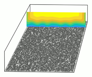
1. Introduction
Rough-wall turbulent boundary layers have been studied extensively for nearly a century (Nikuradse Reference Nikuradse1933; Colebrook & White Reference Colebrook and White1937; Kempf Reference Kempf1937; Schlichting Reference Schlichting1937), however, reliable surface drag prediction remains a challenge. The central difficulty is the boundlessly varying surface morphologies which exist in nature and engineering applications. Though arduous, advancements in fluid dynamic experiments and modelling have steadily provided increased understanding and continue to further engineering capabilities (Chung et al. Reference Chung, Hutchins, Schultz and Flack2021).
Initially the focus of study was drag prediction in pipe flows, but in the 1950s attention turned toward turbulent boundary layers and the search for universal scaling laws, allowing the collapse of a streamwise mean velocity profile onto a single function. That universal function has become known as the law of the wall. After over 50 years of rough-wall boundary layer research, Castro (Reference Castro2007) noted remarkable universality in the ability of the law of the wall to describe the turbulent boundary layer velocity profile across a wide range of rough surfaces. There are two immediate consequences of turbulent boundary layer universality. First, how can it be utilized to build practical engineering models? Second, what are the limits of universality? Both of these questions have been explored in recent years.
For the first question, turbulent boundary layer universality has given hope for the possibility of robust topographic drag prediction models. However, the essential element is understanding how rough surface topography affects roughness length, $y_0$, or the roughness function, $\Delta U^+$, or also sandgrain roughness, $k_s$, which are all measures of rough surface drag. Chung et al. (Reference Chung, Hutchins, Schultz and Flack2021) provides a recent review of studies contributing to this ongoing effort. Most studies have postulated or examined drag prediction algorithms successfully within a small parameter space, however, Chung et al. (Reference Chung, Hutchins, Schultz and Flack2021) highlights that further datasets are required for wider applicability and reduced uncertainty. Specifically, they note the need for an aggregation of systematic studies that sweep through the parameter space or test its limits (http://roughnessdatabase.org/).
For the second question, these drag prediction models, as well as many reduced-order wall-bounded numerical models, implicitly rely on a level of turbulent boundary layer universality. Therefore, knowing the limits of the equation's applicability is vital for high reliability engineering applications. One important theory of turbulent boundary layer universality is Townsend's wall similarity hypothesis. It states that high Reynolds number, fully rough boundary layer turbulence outside of a small roughness layer is independent of the specific surface morphology and statistically similar when appropriately scaled (1976). This hypothesis implies what is known as outer-layer similarity (Raupach, Antonia & Rajagopalan Reference Raupach, Antonia and Rajagopalan1991). Numerous studies have investigated this hypothesis and found significant supporting evidence (Raupach et al. Reference Raupach, Antonia and Rajagopalan1991; Schultz & Flack Reference Schultz and Flack2005; Volino, Schultz & Flack Reference Volino, Schultz and Flack2007; Flack & Schultz Reference Flack and Schultz2014), however, other studies have reported roughness effects well into the outer layer (Krogstad, Antonia & Browne Reference Krogstad, Antonia and Browne1992; Krogstad & Antonia Reference Krogstad and Antonia1999; Volino, Schultz & Flack Reference Volino, Schultz and Flack2011; Hong et al. Reference Hong, Katz, Meneveau and Schultz2012; Placidi & Ganapathisubramani Reference Placidi and Ganapathisubramani2018).
These studies give evidence that, at least under certain circumstances, Townsend's hypothesis does not hold. While researchers are actively working to identify universal criteria for which Townsend's hypothesis holds (Jiménez Reference Jiménez2004; Schultz & Flack Reference Schultz and Flack2005; Flack, Schultz & Shapiro Reference Flack, Schultz and Shapiro2005; Wu & Christensen Reference Wu and Christensen2007; Amir & Castro Reference Amir and Castro2011; Placidi & Ganapathisubramani Reference Placidi and Ganapathisubramani2018), the lack of well-established criteria highlights a lack of understanding of the physics linking surface characteristics to boundary layer statistics. This link is of fundamental scientific and engineering importance due to the prevalence of rough-wall boundary layers and may inform the construction and limits of future drag prediction models.
Very few studies have investigated the effect of regularly vs irregularly arranged roughness elements on the turbulent boundary layer. Researchers have generally focused on regular arrangements because it is easier to isolate important surface statistics or easier to manufacture such surfaces. However, it is not clear if the conclusions drawn from these studies are applicable to flow over random roughness, and irregular or random arrangements are very common in both engineering and nature. Mountainous and hilly topography in the atmospheric boundary layer and barnacles in a ship hull boundary layer are both roughness types that do not appear in the regular arrangements typically investigated. Wind farm inflow often develops over irregular terrain (Stevens & Meneveau Reference Stevens and Meneveau2017) and turbine arrangements often require irregularity due to topography or land use restrictions (Shapiro et al. Reference Shapiro, Starke, Meneveau and Gayme2019; Starke et al. Reference Starke, Meneveau, King and Gayme2021). Even engineered systems contain irregularities. The damaged turbine blade in Bons (Reference Bons2002) has been studied extensively (Wu & Christensen Reference Wu and Christensen2007, Reference Wu and Christensen2010; Mejia-Alvarez & Christensen Reference Mejia-Alvarez and Christensen2010, Reference Mejia-Alvarez and Christensen2013; Barros & Christensen Reference Barros and Christensen2014; Pathikonda & Christensen Reference Pathikonda and Christensen2017) but with little roughness parametric variation except Mejia-Alvarez & Christensen (Reference Mejia-Alvarez and Christensen2010). Research is just beginning to address these limitations. Forooghi et al. (Reference Forooghi, Stroh, Schlatter and Frohnapfel2018) recently conducted a direct numerical simulation (DNS) parametric study with randomly distributed roughness elements but was limited to low Reynolds number due to computational costs. Experimental data at higher Reynolds number are insufficient, and lack of data remains a current limitation in the understanding of rough-wall turbulent boundary layer behaviour.
In recent years, quite a few studies have focused on secondary flows as a way in which turbulent boundary layer universality breaks down. Secondary flows are mean flow features which manifest in the wall-normal spanwise plane (perpendicular to the dominant streamwise flow direction) and have long been studied in non-circular ducts (Nikuradse Reference Nikuradse1930; Hoagland Reference Hoagland1962; Hinze Reference Hinze1967, Reference Hinze1973). Secondary flows were perhaps first noted as a universality concern in rough-wall turbulent boundary layer wind tunnel experiments by Reynolds et al. (Reference Reynolds, Hayden, Castro and Robins2007), who observed spanwise-periodic velocity and turbulence intensity variations in measurements recorded at similar wall-normal distances over staggered cube surfaces. Further inspection revealed that the periodic variation was caused by secondary flow, counter-rotating vortical structures that seemed to correlate with periodic features on the rough surface below. These observations were used to caution about experimental studies with periodic surface features (Reynolds et al. Reference Reynolds, Hayden, Castro and Robins2007). Studies which were to have widely applicable results should try to avoid the presence of such seemingly atypical flow features.
Mostly, it was implicitly assumed that an irregular or random surface would not generate or sustain secondary flows. However, Mejia-Alvarez & Christensen (Reference Mejia-Alvarez and Christensen2013) observed what they described as high-momentum pathways (HMPs) and low-momentum pathways (LMPs) over a multi-scale irregular surface generated from a scaled replica of a damaged turbine blade. They believed that the surface roughness promoted preferential pathways for flow structures that were detectable in the mean flow statistics. Later, Barros & Christensen (Reference Barros and Christensen2014) used extensive stereoscopic (stereo) particle image velocimetry (PIV) data to generate plots of the mean structures in the wall-normal spanwise plane. They observed HMPs and LMPs in the mean streamwise velocity, reduced and enhanced Reynolds shear stress and turbulent kinetic energy in the HMPs and LMPs, respectively, and counter-rotating vortical structures in the signed swirl strength. Barros & Christensen further correlated these mean flow structures with relatively high and low upstream topography in the upstream fetch from the measurement plane. The Barros & Christensen (Reference Barros and Christensen2014) study prompted some important questions for rough-wall turbulence.
Anderson et al. (Reference Anderson, Barros, Christensen and Awasthi2015) provided a possible explanation of the fundamental fluid dynamic mechanisms responsible for generating and sustaining secondary flows within the turbulent boundary layer. In doing so, they were able to draw on the long history of research into non-circular duct secondary flows (Hinze Reference Hinze1967, Reference Hinze1973). Anderson et al. (Reference Anderson, Barros, Christensen and Awasthi2015) used the Reynolds-averaged turbulent kinetic energy balance equation to show that differences in the roughness across the span create spanwise regions that produce more and less turbulent kinetic energy. Their simulations show that HMP and LMP sustainment occurs when the spanwise heterogeneous wall roughness below is streamwise aligned.
Many other researchers have provided some answers to the question of what surface roughness conditions cause secondary flows to form (Willingham et al. Reference Willingham, Anderson, Christensen and Barros2014; Anderson et al. Reference Anderson, Barros, Christensen and Awasthi2015; Vanderwel & Ganapathisubramani Reference Vanderwel and Ganapathisubramani2015; Medjnoun, Vanderwel & Ganapathisubramani Reference Medjnoun, Vanderwel and Ganapathisubramani2018; Yang & Anderson Reference Yang and Anderson2018; Wangsawijaya et al. Reference Wangsawijaya, Baidya, Chung, Marusic and Hutchins2020). They have primarily looked at spanwise heterogeneity either in the form of elevated or recessed streamwise-aligned terrain or streamwise-aligned strips of alternating higher and lower drag-producing roughness. Parametric studies have probed the limits of the parameter space and found that, in general, turbulent boundary layer secondary flows occur when spanwise heterogeneous feature spacing is between approximately $\delta /2$ and $2\delta$, where $\delta$ is the boundary layer thickness. When spanwise spacing is smaller, the features act as homogeneous roughness with effects confined to the roughness sublayer; and when spanwise spacing is larger, the features act as isolated flow perturbations (Vanderwel & Ganapathisubramani Reference Vanderwel and Ganapathisubramani2015; Yang & Anderson Reference Yang and Anderson2018; Wangsawijaya et al. Reference Wangsawijaya, Baidya, Chung, Marusic and Hutchins2020; Chung et al. Reference Chung, Hutchins, Schultz and Flack2021).
The aim of this study is to examine the turbulent boundary layer over varying planform densities of regularly arranged (staggered) and randomly arranged roughness elements, with particular focus on outer similarity and the occurrence and properties of secondary flow structures. Eight planform densities of truncated cone roughness elements in a square staggered pattern were investigated and varied between 10 % and 78 % density. The same planform densities were also investigated with random arrangements of truncated cones. The effect of increasing density on the turbulent boundary layer is determined for both regular and irregular morphologies. No additional spanwise heterogeneity was imposed but is locally present within the random distribution of truncated cones.
Section 2 describes the experimental facility, roughness morphology and flow measuring equipment utilized. Section 3 reports spatially averaged results for both the staggered and random test series at all densities, and differences in turbulent boundary layer parameters are highlighted and examined. Section 4 presents measurements of HMPs and LMPs observed over the irregular arrangements of truncated cones that were not present over the regular staggered arrangements. HMP and LMP correlations with roughness topography are explored, and generation and sustainment mechanisms are discussed. In addition, HMP and LMP turbulent boundary layer parameters and statistics not previously reported in the literature are described. Conclusions are presented in § 5.
2. Experimental details
The experimental approach utilizes a boundary layer water tunnel (§ 2.1) and sixteen test surfaces of staggered and randomly arranged truncated cones (§ 2.2), while measurements are carried out with a laser Doppler velocimetry system described in § 2.3 and a stereo PIV system described in § 2.4.
2.1. Facility
Experiments were conducted at the Hydromechanics Laboratory at the United States Naval Academy in a recirculating boundary layer water tunnel. The test section is nominally 2.00 m long with a 0.20 m wide by 0.10 m tall cross-section at the inlet. The upper wall was adjusted to set a zero pressure gradient, and the resulting acceleration parameter, $K=(\nu /U_e^2)[\textrm {d}U_e/{\textrm {d} x}]$, where $\nu$ is the kinematic viscosity, was less than $5 \times 10^{-9}$ throughout the length of the test section for each test. All tests were conducted at a free-stream velocity of $U_e = 1.25 \ \text {m}\ \text {s}^{-1}$. In this study, ($x, y, z$) were the streamwise, wall-normal and spanwise directions, respectively; $y=0$ was located on the lower surface to which the roughness elements were attached, and $z=0$ was located at the centre of the spanwise cross-section. Test surfaces were mounted on the lower wall of the tunnel. A 0.8 mm diameter wire trip was located 0.20 m from the tunnel inlet and served as the streamwise origin, $x=0$. The roughness field began at $x_r=0.78\ \text {m}$ from the boundary layer trip, and velocity measurements were recorded at $x_0=1.50\ \text {m}$ from the trip which was approximately $18\delta$ from the start of the roughness. A heat pump system controlled fluid temperature to $20 \pm 1^{\circ }\text {C}$ during tests, which in some cases lasted over 50 h.
2.2. Roughness morphology
Sixteen test surfaces were constructed using high resolution additive manufacturing with a Stratasys Objet30 Pro 3D printer. The printer had a lateral resolution of $34\ \mathrm {\mu }\text {m}$ and elevation resolution of $16\ \mathrm {\mu }\text {m}$, which was reported in Flack, Schultz & Barros (Reference Flack, Schultz and Barros2020) from optical profilometer measurements. Since a single test surface exceeds the maximum printable dimensions, each test surface was split into three unique plates for production. Additionally, the subdivided test surfaces were designed with mating features so that there was no discontinuity in the intended topography.
Examples of all sixteen surfaces with their designated names are shown in figure 1. Eight cases had varying planform densities of truncated cone elements in a square staggered pattern (figure 1a–h). In the most dense case, the truncated cone elements were touching but not overlapping at the base. The same eight planform densities were manufactured with random arrangements of the truncated cone elements with no repeating unit over the entire randomized test surface (figure 1i–p). In the random cases, the elements were allowed to overlap, but a minimum of 0.5 mm was maintained between the elements’ upper plateaus. Cases were named with an S for staggered or R for random and then two digit percentage for the planform density.
Selected surface statistics for all sixteen test cases are documented in table 1. Variable $h(x,z)$ is the local surface height. The table provides values for planform density ($\lambda _p$), frontal density ($\lambda _f$), effective slope, mean height $\left \langle h \right \rangle$, height standard deviation ($\sigma _h$), height skewness ($s_k$) and height flatness.
Figure 2 illustrates the calculation of planform and frontal density. Planform density is best illustrated in the figure 2(a,c) top views. Planform density, λp, is calculated from the sum of all truncated cone faces (red, green and blue) projected on the base plane, $A_p$, then divided by the base lot area, $A_0$, so that $\lambda _p=A_p/A_0$. Frontal density, $\lambda_f$, is calculated by the sum of all upstream facing surfaces (red and green) projected on a plane normal to the streamwise direction, $A_f$, then divided by the base lot area, $A_0$, so that $\lambda _f=A_f/A_0$. There are no differences between the red and green surfaces, the green surfaces were simply chosen to illustrate the area projection. Selected truncated cone upstream facing surfaces in green illustrate the projection on the plane normal to flow in the figure 2(b,d) isometric views. All upstream facing surfaces, regardless of whether they may be sheltered by the wake of upstream elements, are included in the frontal density calculation. As seen in figure 2(d) for random plates, truncated cones were allowed to overlap on the base lot area. This causes a solid surface occlusion of the front face of the downstream overlapping truncated cone. The occluded area is not included in the frontal density calculation as seen in the projection.
All truncated cone elements were identical, with the geometry documented in figure 3. Truncated cone dimensions were selected to idealize a single barnacle. Understanding boundary layers over barnacle roughness is important for informing drag prediction models and understanding ship propulsion requirements. However, these truncated cone elements may also be a proxy for low mountainous terrain in the atmospheric boundary layer. Specific truncated cone ratios were selected based on detailed barnacle statistics from Spivey (Reference Spivey1988). The ratio of height to base diameter is lower than the average reported by Spivey (Reference Spivey1988) but still falls within the standard deviation. Also, experimental and computational fluid dynamic studies which focused on barnacle elements were reported by Schultz, Kavanagh & Swain (Reference Schultz, Kavanagh and Swain1999) and Sadique (Reference Sadique2016). These studies measured barnacles with an average of $k=0.49D$ and $k=0.37D$ respectively, where $D$ is the base diameter and $k=\max (h)$ is the uniform height of the roughness crests. The ratio studied here falls between these two values.
2.3. Laser Doppler velocimetry measurements
Detailed boundary layer velocity statistics were recorded with a TSI FSA3500 two-component laser Doppler velocimetry (LDV) system measuring streamwise and wall-normal velocity. A custom beam displacer and beam expander produce ellipsoidal measurement volumes that have a beam waist of $45 \ \mathrm {\mu } \text {m}$. The flow was seeded with $2 \ \mathrm {\mu } \text {m}$ diameter silver coated glass spheres. For the square staggered cases, wall-normal profiles were recorded at nine locations over a repeating unit as seen in figure 4. Each of the nine staggered-case profiles contained 50 sampling locations in the wall-normal direction where velocity data were recorded for 180 s. The nine locations were representative of the entire repeating unit by utilizing mirroring and translation. Mirroring is the assumption that streamwise and wall-normal velocity component statistics on the left side of an upstream element are similar to those on the right side of the element. Translation is the assumption that velocity statistics from one profile are similar to another within the repeating unit that has the same relative position to a nearby elements (e.g. all profiles in the repeating unit centred over an element are similar). Then, an area weighting was used to create a spatial-averaged profile for all time-averaged statistics.
For the random cases, 12 wall-normal profiles were recorded and spaced at $1.5D$ across the span of the tunnel. The red profiles in figure 5 show these 12 locations. The spacing and number of profiles allowed independent profiles and well-converged spatial averages across the span. Additional wall-normal profiles were performed for the R17 and R39 cases with 23 profiles spaced at $0.75D$ since these cases appeared less well converged when using 12 profiles. The additional 11 profiles for these test cases are depicted in blue on figure 5. Each of the 12 or 23 random-case profiles contained 50 sampling locations in the wall-normal direction where velocity data were recorded for 150 s. The field of view was $115 \ \text {mm} \times 52 \ \text {mm}$ in the spanwise and wall-normal directions, respectively. All time-average statistics were calculated using a virtual saturable-detector scheme with $5\ \text {ms}$ saturation. Due to the amount of data sampled, all of these tests were over 24 h in duration.
2.4. Stereoscopic PIV measurements
In order to investigate mean flow structures, stereoscopic PIV measurements were employed in the wall-normal spanwise ($y, z$) plane at $x=1.55\ \text {m}$ downstream of the trip, which approximately matches the downstream location used in the LDV measurements. Measurements were recorded over the least dense and most dense cases for both staggered and random surfaces (S10, S78, R10, R78).
For each surface, a wall-normal spanwise plane was acquired at the spanwise centre of the test section. The flow was seeded with the same particles used in the LDV measurements. For each plane, 1000 image pairs were acquired using two CCD cameras with $3320 \times 2496$ pixel arrays. The acquisition frequency was low (approximately $3\ \text {Hz}$), so the image pairs were statistically independent. The time interval between images in each pair was $200 \ \mathrm {\mu } \text {s}$, which at the free-stream velocity corresponds to a $0.25 \ \text {mm}$ displacement in the streamwise direction. Velocity vectors were obtained with TSI Insight 4G software using 32 pixel square windows with 50 % overlap. The field of view was $81 \ \text {mm} \times 40 \ \text {mm}$ in the spanwise and wall-normal directions, respectively. The spatial resolution of the PIV velocity vectors was 0.4 mm, which compares with the $300\ \mathrm {\mu }\text {m}$ length of the LDV probe volume.
3. Spatial-averaged results
This section presents spatial-averaged results for all staggered and random truncated cone surfaces. Spatial averaging is computed over the basic repeating tile for the staggered cases and in the spanwise direction for the random cases. Friction velocity, roughness length and zero-plane displacement are determined as functions of the planform density parameter space and trends are discussed. Two existing a priori drag prediction models are evaluated against the results. The section concludes by highlighting differences between turbulent boundary layer profiles and parameters between the staggered and random surfaces which indicated a breakdown in outer-layer similarity.
3.1. Spatial-averaged boundary layer profile results
Spatial-averaged experimental boundary layer profiles were analysed with the comprehensive shear stress (CSS) method described in Womack, Meneveau & Schultz (Reference Womack, Meneveau and Schultz2019). The CSS method calculates several important turbulent boundary layer parameters appearing in the log-law equation. The log-law equation with the wake function is
In this equation, $U$ is the mean streamwise velocity. The velocity scaling parameter is the friction velocity, $u_\tau$, and the $+$ superscript indicates normalization by $u_\tau$; $\kappa =0.384$ is the Kármán constant used throughout this study with corresponding smooth-wall intercept, $A=4.17$ (Chauhan, Nagib & Monkewitz Reference Chauhan, Nagib and Monkewitz2007). Zero-plane displacement, $d$, is a shift in the effective origin of the log law due to roughness; $y_0$ is known as the roughness length and is related to the roughness function by $\Delta U^+ = A + (1/\kappa ) \ln { ( y_0 u_\tau /\nu )}$ or to the equivalent sandgrain roughness by $k_s = y_0 \textrm {e}^{8.5 \kappa }$ (Jiménez Reference Jiménez2004; Castro Reference Castro2007; Chung et al. Reference Chung, Hutchins, Schultz and Flack2021). Friction velocity ($u_\tau$), wall shear stress ($\tau _w$) and skin friction ($c_f$), will all be used interchangeably based on application and are related by definition $u_\tau \equiv \sqrt {\tau _w/\rho } \equiv U_e \sqrt {c_f/2}$, where $U_e$ is the free-stream velocity and $\rho$ is the fluid density. The wake function, $W(y/\delta )$, models the outer-region deviation from the log law and scales with the boundary layer thickness. This study will use the most common definition of the boundary layer thickness, $\delta$, namely the wall-normal distance where velocity reaches 99 % of the free-stream velocity (so that $U(\delta ) =0.99U_e$). The wake strength parameter, $\varPi$, measures the strength of the deviation by $\varPi = ({\kappa }/{2}) \max [ U^+ ( y ) - ({1}/{\kappa }) \ln ( y/y_0 ) ]$.
The extended Volino & Schultz equation is a reformulated total shear stress balance and was fit in the range of $0.15 < (y-d)/(\delta -d) < 0.30$ to determine $u_\tau$, and the log-law equation was fit in the range of $0.07 < y/\delta < 0.15$ to determine $y_0$ and $d$ in each iteration (Volino & Schultz Reference Volino and Schultz2018; Womack et al. Reference Womack, Meneveau and Schultz2019). An iterative solution process is required since both equations have dependencies in all three variables. The convergence criteria for each profile were three significant digits in $u_\tau$, $y_0$ and $d$ or 10 iterations. Table 2 contains results from the CSS method as well as other relevant profile parameters for each surface's average profile. Displacement thickness, $\delta ^*$, and momentum thickness, $\theta$, were calculated assuming an extrapolation of the log law between $y=y_0+d$ and the nearest measurement point to the wall (Castro Reference Castro2007). Also, relative roughness height, $k/\delta$ is reported and shows that the relative roughness height is between $0.08 < k/\delta < 0.10$ in all cases. Finally, friction Reynolds number, ${\textit {Re}}_\tau \equiv \delta ^+ \equiv u_\tau \delta / \nu$ is reported for each case.
The friction velocity is one of the most important parameters to determine. The CSS method determines friction velocity indirectly, so it is prudent to check results against expectations. Figure 6 shows the spatial-averaged LDV results for skin friction plotted against the skin-friction law first derived by Clauser (Reference Clauser1954) and Rotta (Reference Rotta1962) from the log-law equation. The skin-friction law can be written, as in Castro (Reference Castro2007), as
and provides a relationship between skin friction and the momentum thickness normalized by roughness length. Here, $H$ is the shape factor defined as $H=\delta ^*/\theta$. The two plotted curves, one with $\varPi =0.55$ and one with $\varPi =0.70$, require an assumed wake function to solve for shape factor and are described in detail in Castro (Reference Castro2007) and Womack et al. (Reference Womack, Meneveau and Schultz2019). The random cases’ results are observed to be closer to the $\varPi =0.55$ curve, and the staggered cases’ results tend to lie closer to the $\varPi =0.70$ curve. This is consistent with the wake strength results found in table 2 which shows the random cases tend to have results near $\varPi =0.55$ and the staggered cases tend to have higher wake strengths in the spatial-averaged profiles.
Inner-normalized, spatial-averaged mean streamwise velocity profiles are plotted in figure 7. Figure 7(a) shows the staggered cases, and figure 7(b) shows the random cases. The dashed black line shows the smooth-wall log law. All profiles show the expected downward shift due to roughness effects. The S10, R10, S17 and R17 cases have clearly less downward shift than the other cases, which plot together more closely. All sixteen average profiles exhibit a log–linear region with slope of approximately $1/\kappa$ between approximately $0.07 < y/\delta < 0.15$ (approximately $100 \lesssim (y-d)^+ \lesssim 300$). The existence of a linear region in the spatial-averaged profile with this roughness height to boundary layer thickness ratio or larger has been seen in other recent studies such as Cheng & Castro (Reference Cheng and Castro2002), Placidi & Ganapathisubramani (Reference Placidi and Ganapathisubramani2015, Reference Placidi and Ganapathisubramani2018) and Yang et al. (Reference Yang, Sadique, Mittal and Meneveau2016) among others. The process of solving for $y_0$ and $d$ assumed this linear region existed, however, the extent of such a region is not necessarily guaranteed in all cases.
Figure 8 shows inner-normalized spatial-averaged mean Reynolds shear stress profiles for all sixteen cases. Staggered cases are in figure 8(a), and random cases are in figure 8(b). The profiles appear consistent with data from other rough surfaces such as Cheng & Castro (Reference Cheng and Castro2002), Flack, Schultz & Connelly (Reference Flack, Schultz and Connelly2007), Flack & Schultz (Reference Flack and Schultz2014) and Placidi & Ganapathisubramani (Reference Placidi and Ganapathisubramani2015, Reference Placidi and Ganapathisubramani2018, Reference Placidi and Ganapathisubramani2019). However, there are notable differences between the cases in the near-wall region, $(y-d)/(\delta -d)<0.15$. This is attributed to the significant spatial heterogeneity found in this turbulence statistic in the roughness sublayer, defined as the region where local Reynolds shear stresses differ by greater than 10 %. Flack et al. (Reference Flack, Schultz and Connelly2007) and Placidi & Ganapathisubramani (Reference Placidi and Ganapathisubramani2015) both report that the roughness sublayer in their experiments extended up to $y\approx 5k$. It is likely that the nine profiles of the staggered cases and twelve (or 23) profiles of the random cases do not provide a fine enough resolution to capture a well-converged spatial-averaged Reynolds shear stress in this region, similar to the results of Cheng & Castro (Reference Cheng and Castro2002) and Placidi & Ganapathisubramani (Reference Placidi and Ganapathisubramani2015). The CSS method, which was used to calculate $u_\tau$, $y_0$ and $d$, avoids uncertainty in the region by only fitting the extended Volino & Schultz equation to Reynolds shear stress and dispersive shear stress in the range of $0.15 < (y-d)/(\delta -d) < 0.30$.
Reynolds number independence of the rough surface drag was not checked directly, however, several important reviews consider rough-wall boundary layers Reynolds number independent when $k_s^+ \gtrsim 100$ (Raupach et al. Reference Raupach, Antonia and Rajagopalan1991; Jiménez Reference Jiménez2004; Flack et al. Reference Flack, Schultz and Shapiro2005). Table 2 shows that all cases from this study are at least 45 % greater than this threshold, so Reynolds number independence is expected and $y_0$ and $k_s$ are solely a function of the surface roughness.
Normalized roughness length, $y_0/k$, as a function of planform density, $\lambda _p$, was investigated and results are plotted in figure 9. Normalized roughness length for staggered and random cases at equivalent planform densities plot closely together for all but one density, $\lambda _p=0.70$. Specific selection of the linear range used to fit the log-law equation is the largest source of error for determination of these average profile parameters. Therefore, error bars were generated by varying the region in which the linear regression was fit to the log law during iteration in the CSS method. Those assumed linear regions also fit in the CSS method were: $0 < y/\delta < 0.15$, $0.10 < y/\delta < 0.15$, $0 < y/\delta < 0.19$, $0.07 < y/\delta < 0.19$ and $0.10 < y/\delta < 0.19$. As noted by Placidi & Ganapathisubramani (Reference Placidi and Ganapathisubramani2015) and Womack et al. (Reference Womack, Meneveau and Schultz2019), fitting of (3.1) for $y_0$ and $d$ carries significant uncertainty, however, it is still common to use a fitting procedure due to lack of a better alternative when only velocity profile measurements are available. Additionally, using a consistent fitting procedure allows for comparison among cases which provides valuable insight into roughness length trends. Varying the region in which the extended Volino & Schultz equation was fitted had a much smaller effect and was not included in the results presented here.
Since staggered and random cases plot so close together, the results suggest that normalized roughness length is more a function of the density and element shape rather than their particular arrangement. This may be due to relatively comparable average distances between elements at each density in the staggered and random configurations. The correlation could break down if there was significant element clustering or directionality at the same density (Forooghi et al. Reference Forooghi, Stroh, Magagnato, Jakirlić and Frohnapfel2017; Anderson Reference Anderson2020; Chung et al. Reference Chung, Hutchins, Schultz and Flack2021). Truncated cone surfaces tested in this study show increasing normalized roughness length in the range $0 < \lambda _p \lesssim 0.4$. Then a gradual decrease above $\lambda _p \gtrsim 0.4$. To the authors’ knowledge, the only truncated cone data that provide comparison over a range of planform densities are found in Sadique (Reference Sadique2016). He conducted large eddy simulations over staggered and aligned truncated cones at several planform densities. The comparison study's repeating truncated cone had height $k=0.5D$ and plateau diameter equal to $0.5D$, making it slightly taller and wider than the truncated cone in this study. The results compare well with the present study given the differences in truncated cone shape. The normalized roughness length magnitudes are generally consistent, and if a curve were drawn though these points, it would seem to indicate a peak normalized roughness length around $\lambda _p \approx 0.4$ as the current experimental data suggest.
Most other studies which have systematically varied planform density have used cubes, rectangular prisms or rectangular LEGO® blocks including Hall, Macdonald & Walker (Reference Hall, Macdonald and Walker1996), Cheng et al. (Reference Cheng, Hayden, Robins and Castro2007), Hagishima et al. (Reference Hagishima, Tanimoto, Nagayama and Meno2009), Placidi & Ganapathisubramani (Reference Placidi and Ganapathisubramani2015, Reference Placidi and Ganapathisubramani2018), Yang et al. (Reference Yang, Sadique, Mittal and Meneveau2016) and Zhu et al. (Reference Zhu, Iungo, Leonardi and Anderson2017). Most of these studies suggest a peak drag at a density of $\lambda _p \approx 0.15$ and marked drop in drag at higher densities, so the curve shape is not similar to the results reported here or in Sadique (Reference Sadique2016). Additionally, most a priori analytical models were designed and evaluated against these rectangular prism surface morphologies (often called urban-like roughness) and were not found to be easily adaptable to truncated cone surface elements.
A roughness length model in Macdonald, Griffiths & Hall (Reference Macdonald, Griffiths and Hall1998), however, was found to be adaptable to the truncated cone shape when provided an a priori estimate for the coefficient of drag, $C_{DH}$, and zero-plane displacement height, $d$. Two relevant coefficient of drag measurements were found in a literature survey. Sadique (Reference Sadique2016) reports $C_D=0.23$ from DNS on truncated cones in a laminar boundary layer; $C_D$ corresponds with $C_{DH}=0.27$ when using the Blasius laminar profile solution to estimate velocity at the roughness crests, $U_H$, from reported simulation details. Additionally, Schultz et al. (Reference Schultz, Kavanagh and Swain1999) reported a coefficient of drag of $C_D=0.52$ for natural barnacle specimens in a turbulent boundary layer; $C_D$ corresponds with $C_{DH}=0.65$ when using reported information to estimate $U_H$ in a turbulent boundary layer. Neither reported coefficient of drag was an ideal match for this study. Sadique (Reference Sadique2016) had a similar truncated cone element but differing laminar flow regime. Schultz et al. (Reference Schultz, Kavanagh and Swain1999) had a similar turbulent flow regime but differing natural barnacle element. Therefore, both were used for comparative results. Details on the adaption of the Macdonald et al. (Reference Macdonald, Griffiths and Hall1998) model and a priori estimation of $d$ for truncated cones are included in Appendix A.
Results for these two values of $C_{DH}$ are shown in figure 9. The curve, which utilizes $C_{DH}=0.65$, performs well below $\lambda _p \approx 0.4$ but does not peak there as the experimental data suggest. Instead, it seems to calculate a fairly flat peak around $\lambda _p \approx 0.55$ which is above the measurements and outside of their uncertainty. The curve which utilizes $C_{DH}=0.27$ consistently plots below the experimental results. This confirms that the model is sensitive to an accurate estimate of an individual element's coefficient of drag and limits the a priori reliability of the model on many surface morphologies where the coefficient of drag is not known well or roughness shapes are not consistent.
Surface statistical models provide another possible a priori prediction of normalized roughness length. These types of models have the advantage of not requiring estimation of surface parameters like $C_{DH}$ and $d$. Zhu et al. (Reference Zhu, Iungo, Leonardi and Anderson2017), inspired by the contribution of Flack & Schultz (Reference Flack and Schultz2010), provides an explicit expression for $y_0$ as a function of the surface standard deviation and skewness,
where constants $\alpha$ and $\beta$ are $0.1$ and $0.9$, respectively. The truncated cone surfaces tested in this study have a slightly different standard deviation and skewness at each density due to the overlapping truncated cones on the random plates. Therefore, this model produces a range of results for the planform densities tested. This range is plotted in figure 9 as the dark grey shaded area. The Zhu et al. (Reference Zhu, Iungo, Leonardi and Anderson2017) equation roughly matches the slope of the current experiments but underestimates the normalized roughness length above $\lambda _p \gtrsim 0.4$. It also does not seem to capture the shape of the curve well and overestimates the normalized roughness length below $\lambda _p \lesssim 0.4$. For sparse distributions of individual elements, a simple calculation in the limit $\lambda _p \to 0$ shows that $\sigma ^2 \to k^2 \lambda _p$ while $s_k \sim \lambda _p^{-1/2}$. Thus the predicted $y_0$ based on the skewness, $s_k$, does not tend to zero when $\lambda _p \to 0$ but to a constant fraction of $k$ (for $\beta =1$), consistent with the Zhu et al. (Reference Zhu, Iungo, Leonardi and Anderson2017) results shown in figure 9.
Since (3.3) seems to match the shape of the profile and Zhu et al. (Reference Zhu, Iungo, Leonardi and Anderson2017) report $\alpha \approx 0.1$, it seems reasonable to attempt to tune $\alpha$ for a better fit. Additionally, Zhu et al. (Reference Zhu, Iungo, Leonardi and Anderson2017) cite several studies where $0.1 < \alpha < 0.17$ bounds the reported values. Equation (3.3) yields a good fit to the data above $\lambda \gtrsim 0.4$ when $\alpha =0.14$ as seen by the light grey shaded area in figure 9.
Given the success of the Macdonald et al. and Zhu et al. models at different surface densities and their different underlying assumptions, it is reasonable to postulate that the truncated cone surface is exhibiting two different flow regimes. The Macdonald et al. model assumes a coefficient of drag for individual elements while the Zhu et al. model attempts to characterize the surface with surface statistics. Below $\lambda _p \lesssim 0.4$ the flow is characteristic of flow around isolated elements, while above $\lambda _p \gtrsim 0.4$ the flow is characteristic of skimming flow over a rough surface with the transition happening at the point of peak drag. Such a transition was expected as this type of behaviour has been observed before in other studies such as Grimmond & Oke (Reference Grimmond and Oke1999) and Placidi & Ganapathisubramani (Reference Placidi and Ganapathisubramani2015). However, proposed flow regime prediction parameters such as ratios of roughness height to average distance between elements are difficult to apply to truncated cones. This is due to their varying cross-section with height, which gives rise to different flow behaviour as $\lambda _p \to 1$. Cubes tend to a smooth wall as $\lambda _p \to 1$ leading to skimming behaviour whereas truncated cones have a dense rough surface as $\lambda _p \to 1$ with evidence of limited sheltering at the tested dimensional ratios.
Normalized zero-plane displacement height, $d/k$, is plotted in figure 10. Based on flow physics and previous studies, it is expected that $d/k$ increases with planform density Grimmond & Oke (Reference Grimmond and Oke1999). Such a trend is visible at larger $\lambda _p$ while the trend is somewhat noisy at $\lambda _p<0.4$.
3.2. Differences in spatial-averaged staggered and random surface profiles
Local outer-normalized mean streamwise velocity profiles for the S78 staggered case are plotted in figure 11(a), and local outer-normalized mean streamwise velocity profiles for the R78 random case are plotted in figure 11(b). Cases S78 and R78 were selected to showcase the trends seen for all staggered and random cases, respectively. The spatial average is plotted with a thick black line. It is clear from figure 11(a) that the various S78 local profiles converge within one roughness height, $k$, above the roughness crests ($(k-d)/(\delta -d)=0.12$ for this case). Reynolds shear stress profiles (not shown) converge within $2k$ above the roughness crests. This is the result for all staggered cases and consistent with other studies that report convergence above $y > 5k$ (Flack et al. Reference Flack, Schultz and Connelly2007; Placidi & Ganapathisubramani Reference Placidi and Ganapathisubramani2015). In contrast, figure 11(b) shows visual differences in the local profiles all the way to the edge of the boundary layer.
Inner-normalized mean streamwise velocity profiles in defect form are included for all staggered cases in figure 12(a) and for all random cases in figure 12(b). DNS at ${\textit {Re}}_\tau \approx 2000$ from Sillero, Jiménez & Moser (Reference Sillero, Jiménez and Moser2013) is included as the thick black dotted line for reference in both plots. It can be observed that all staggered cases except S10 plot above the DNS reference in figure 12(a), and all random cases plot near the DNS reference in figure 12(b). Additionally, there is a greater visual spread in the profiles at low $(y-d)/(\delta -d)$ for the staggered cases when compared with the random cases.
Further evidence of the differences seen in figure 12 is observed in the column of $\varPi$ values in table 2. For the staggered cases, wake strength is in the range $\varPi =0.53 - 0.79$ compared with $\varPi =0.51 - 0.66$ for the random cases, and the differences in wake strength are largely outside of the experimental uncertainty when compared at similar $\lambda _p$, as seen in figure 13(a). Additional comparison with other surface morphologies such as the mesh, cubes, rectangular blocks and sandgrain surfaces from Castro (Reference Castro2007) in figure 13(b) reveals that the staggered cases seem to show wake strengths commensurate with the roughness function. However, the random cases appear to have reduced wake strength by comparison.
As suggested by the varying wake strength, outer-layer similarity in the spatially averaged profiles is not observed across the range of densities of either the staggered or random arrangements of truncated cones. Neither the criterion from Jiménez (Reference Jiménez2004) of $k/\delta <0.025$ or the criterion from Flack et al. (Reference Flack, Schultz and Shapiro2005) of $k_s/\delta <0.025$ would have predicted outer-layer similarity. However, Amir & Castro (Reference Amir and Castro2011) suggest that boundary layers exhibit outer-layer similarity when $k/\delta <0.15$, and the present measurements do meet this criterion. Furthermore, each staggered case, when compared with the random case at the same density in figure 13(a), show roughly equivalent measures of $k/\delta$ or $k_s/\delta$ but have values of $\varPi$ which are different (see table 2). The findings here are consistent with Placidi & Ganapathisubramani (Reference Placidi and Ganapathisubramani2018), where outer-layer similarity did not solely depend on $k/\delta$ or $k_s/\delta$ but must also depend on other characteristics of the surface morphology. The presently observed differences in the outer layer over surfaces with similar densities and roughness height ratios adds interesting new evidence to the salient surface morphology parameters which generate or disrupt outer-layer similarity.
Notably, the observations in figures 12 and 13 were formed on spatial-averaged profiles. However, there was significant spatial variation across the horizontal tunnel span ($z$-direction) on all random surface cases that was illustrated by the R78 case in figure 11(b). In contrast, the staggered surface cases, as shown in the S78 case in figure 11(a), showed variation only in the near-wall region consistent with other studies (Raupach et al. Reference Raupach, Antonia and Rajagopalan1991; Jiménez Reference Jiménez2004; Flack et al. Reference Flack, Schultz and Shapiro2005; Amir & Castro Reference Amir and Castro2011). The lack of collapse of the profiles in figure 11(b) outside of the inner layer is striking given that all of these profiles were recorded over a similar surface at the same Reynolds number, ${\textit {Re}}_x = U_e x/\nu$. Taken together, these observations indicate a breakdown in outer-layer similarity warranting further analysis. In § 4, it will be shown that these differences can be attributed to secondary flows which create HMPs and LMPs and disrupt outer-layer similarity.
4. Secondary flow structures and their characteristics
This section presents an analysis of the deviations from outer-layer similarity and the secondary flow structures that generate HMPs and LMPs observed to occur over the random truncated cone surfaces. Section 4.1 shows evidence of HMPs and LMPs over the present random surfaces, consistent with observations from previous studies. However, evidence for HMPs and LMPs appears much weaker for flow over the staggered surfaces. This stands in contrast to previous studies where spanwise flow heterogeneity is normally observed over surfaces with spanwise roughness periodicity. Section 4.2 attempts to correlate local surface elevation with the momentum pathways. Section 4.3 compares local turbulent boundary layer profiles with measures of turbulent boundary layer universality. Lastly, § 4.4 examines turbulent shear stress differences in HMPs and LMPs through quadrant analysis and compares with other reported data.
4.1. Evidence of secondary flow structures
Figures 14 and 15 show the wall-normal spanwise plane of mean streamwise velocity at $x=1.50\ \text {m}$ surveyed with the LDV system. Figure 15(a–g) shows contour plots created from the 12 or 23 profiles described in § 2.3 and shown in figure 5, and plots in figures 14 and 15(h) show surveys of the entire tunnel span with linear grid spacings in the wall-normal and spanwise directions.
The smooth-wall survey in figure 14 displays a typical smooth-wall boundary layer that has developed in a rectangular tunnel. There are notable distortions in the corners as expected due to the square tunnel corners and a slight (1–2 mm or $\pm 0.04\delta$) thickening of the boundary layer near the middle of the span (Nikuradse Reference Nikuradse1926, Reference Nikuradse1930; Prandtl Reference Prandtl1927; Hoagland Reference Hoagland1962; Hinze Reference Hinze1967, Reference Hinze1973). These are due to small tunnel-scale secondary flows typical of a tunnel with these dimensions and are generally considered negligible for most boundary layer results.
In contrast, all random cases shown in figure 15 display mean streamwise velocity heterogeneity across the tunnel span. The spanwise heterogeneity consists of alternating HMPs and LMPs. HMPs and LMPs exist in the time-averaged streamwise velocity and are different from high-momentum regions and low-momentum regions which are instantaneous flow features (Mejia-Alvarez & Christensen Reference Mejia-Alvarez and Christensen2013; Barros & Christensen Reference Barros and Christensen2014).
For further evidence of the marked difference in spanwise heterogeneity, figures 16 and 17 show measures of the streamwise velocity deviation from the spanwise average. Figure 16 visualizes the streamwise velocity less the spanwise-average mean velocity for selected cases. The deviations up to $\pm 10\,\%$ are readily apparent. Figure 17 plots the standard deviation of mean streamwise velocity across the span at all measured wall-normal distances. For this calculation, the spanwise extent was limited to that available for all random surfaces (i.e. the edge effects recorded on the smooth wall were excluded and the 12 profile R78 test was used). The standard deviation represents a quantitative measure of the spatial variability and is essentially the square root of the streamwise component of the dispersive stress. In figure 17(b), it is readily seen that the mean streamwise velocity standard deviation is 2 to 5 times higher across the span for the random cases (figure 15) when compared with the smooth wall (figure 14) in much of the boundary layer. Also included in figure 17(a) is the standard deviation for the nine profiles of each staggered case. These nine profiles were not across the span but show the difference in standard deviation across all truncated cone cases (i.e. quantify the difference between figure 11a,b). Finally, it is notable that there is no trend with respect to density evident in the standard deviation, which appears consistent with figure 15.
There are a few unique observations that can be gained from LDV measurements over these surfaces. Figure 18 shows three planes of mean streamwise velocity data for the R78 case. Each of these planes contains six profiles spaced $1.5D$ in the $z$-direction and centred on the span. The middle plane is located at $x=1.50\ \text {m}$ and is co-located with other wall-normal spanwise measurements. The upstream and downstream planes are located $\pm 8\ \text {cm}$, approximately $2\delta$, from the centre plane. The three planes show similar contours which indicates that these HMPs and LMPs exist over a streamwise distance of more than $4\delta$. It is noted that Mejia-Alvarez & Christensen (Reference Mejia-Alvarez and Christensen2013) measured $1\delta$ sustainment over their irregular surface. This indicates that the secondary flow structures creating the HMPs and LMPs are longer standing than previously reported over an irregular or random surface.
In figure 19(a), the repeatability of the results is examined by comparing results from different experiments over the same surface. The R78 case full-span linearly spaced mean streamwise velocity from figure 15(h) is shown again in two dimensions in the upper plot. Overlaid in black is the R78 test which measured independently the 12 profiles also shown in figure 5. Overlaid in red on this figure are data contours from the co-located middle plane in figure 18 from yet a different experiment. This plot highlights the location repeatability of the HMPs and LMPs over these surfaces by showing that the HMPs and LMPs appear in the same locations on independent test runs.
Figure 19(b) shows the R78 case full-span Reynolds shear stress data. This plot gives further evidence of HMPs and LMPs since it demonstrates depressed and elevated levels of Reynolds shear stress coincident with HMPs and LMPs respectively as was shown in both Barros & Christensen (Reference Barros and Christensen2014) and Anderson et al. (Reference Anderson, Barros, Christensen and Awasthi2015). Again, the 12 profile test and the 6 profile test at $x=1.50\ \text {m}$ were overlaid in black and red respectively, and the elevated and depressed levels of Reynolds shear stress were measured in the same spanwise locations. The location repeatability across independent test runs suggests some correlation with the surface roughness which will be discussed in § 4.2.
Further measurements were acquired with stereo PIV in order to measure all three velocity components and also to compare staggered test surfaces and random test surfaces with the same measurement system on a subset of roughness density cases. The least dense and most dense cases were selected for these measurements. Figure 20 shows contour plots of outer-normalized streamwise velocity ($U/U_e$), signed swirling strength ($\overline {\varLambda _{ci}} ( \delta / U_e )$), Reynolds shear stress ($-\overline {u'v'}/U_e^2$) and turbulent kinetic energy ($tke/U_e^2$) from R10, R78, S10 and S78, respectively. Turbulent kinetic energy is defined as $tke\equiv (1/2)\,(\overline {u'^2}+\overline {v'^2}+\overline {w'^2}$). Signed swirling strength, $\overline {\varLambda _{ci}} ( \delta / U_e )$, is an ensemble-averaged quantity, where $\varLambda _{ci}=\lambda _{ci} ( \omega _x / | \omega _x | )$ and $\lambda _{ci}$ is the imaginary part of the complex-conjugate eigenvalue of the instantaneous velocity gradient tensor and is a frame-independent measure of the local rotation (Adrian, Christensen & Liu Reference Adrian, Christensen and Liu2000; Barros & Christensen Reference Barros and Christensen2014; Vanderwel & Ganapathisubramani Reference Vanderwel and Ganapathisubramani2015; Vanderwel et al. Reference Vanderwel, Stroh, Kriegseis, Frohnapfel and Ganapathisubramani2019). Swirl is closely related to vorticity and is the part of the vorticity due to rotation as opposed to shear.
The R10 and R78 streamwise velocity contours plotted in figures 20(a) and 20(b) clearly show similar spanwise variations that were observed previously now in stereo PIV measurements and indicate alternating HMPs and LMPs. In contrast, the streamwise velocity for the staggered (regular) S10 and S78 cases is far more homogeneous in the spanwise direction. For the $\lambda _p=0.10$ cases, the spanwise standard deviation of the outer-normalized mean streamwise velocity at $y/\delta =0.25$ in the range $-1.3< z/\delta <1.3$ is $3.8 \times 10^{-2}$ for the random case (R10) while it is only $1.7 \times 10^{-2}$ for the staggered case (S10). For the $\lambda _p=0.78$ cases, the standard deviation values are $4.1 \times 10^{-2}$ for R78 and only $1.5 \times 10^{-2}$ for S78.
The signed swirl strength measurements shown in figures 20(e) and 20(f) exhibit spanwise heterogeneous variations with peak values centred between the HMPs and LMPs, and sign changes at the HMPs and LMPs (at the dashed lines). This is indicative of the $\delta$-scale secondary flows which rotate clockwise in positive $\overline {\varLambda _{ci}}$ (red) and counter-clockwise in negative $\overline {\varLambda _{ci}}$ (blue) regions. These counter-rotations sweep high-momentum fluid from higher in the boundary layer downward in the HMPs and eject low-momentum fluid from deep in the boundary layer upward (Barros & Christensen Reference Barros and Christensen2014; Anderson et al. Reference Anderson, Barros, Christensen and Awasthi2015). Optical distortions above $y/\delta >0.75$ masked the trends observed closer to the wall and are not shown. While the swirl strength measurements are affected to some degree by experimental error of the stereo PIV system, the differences visible between the random and staggered cases are outside experimental error.
Lastly, Reynolds shear stress contour plots in figures 20(i) and 20(j) show reduced and enhanced Reynolds shear stress in the HMPs and LMPs, respectively, and turbulent kinetic energy contour plots in figures 20(m) and 20(n) show evidence of reduced and enhanced $tke$ in the HMPs and LMPs, respectively. Simulations in Anderson et al. (Reference Anderson, Barros, Christensen and Awasthi2015) indicated that enhanced Reynolds shear stress and $tke$ in the LMPs were a result of a local $tke$ production–dissipation imbalance at the surface (specifically below the HMPs) and $tke$ advection into the LMPs rather than local $tke$ production. As with the LDV results, the results based on present stereo PIV measurements are consistent with those of Barros & Christensen (Reference Barros and Christensen2014) and Anderson et al. (Reference Anderson, Barros, Christensen and Awasthi2015) (Womack Reference Womack2021, § 3.4.3). Additionally, the results are consistent with simulations of Stroh et al. (Reference Stroh, Schäfer, Frohnapfel and Forooghi2020) and the discussion in Medjnoun, Vanderwel & Ganapathisubramani (Reference Medjnoun, Vanderwel and Ganapathisubramani2020) for strip-type roughness, where streamwise-coherent spanwise heterogeneity consists of changes in surface drag rather than topographical elevation (ridge-type). However, while the truncated cone data presented here are consistent with Anderson et al. (Reference Anderson, Barros, Christensen and Awasthi2015), Medjnoun et al. (Reference Medjnoun, Vanderwel and Ganapathisubramani2020) and Stroh et al. (Reference Stroh, Schäfer, Frohnapfel and Forooghi2020), evidence from Stroh et al. (Reference Stroh, Schäfer, Frohnapfel and Forooghi2020) indicates that Anderson et al. (Reference Anderson, Barros, Christensen and Awasthi2015) does not provide a complete description of the mechanisms generating secondary flows over rough surfaces particularly when ridge-type roughness is present.
The dispersive shear stress was also calculated for both the random and staggered cases from stereo PIV data, and these results corroborate the discussion of the secondary flows above. In the random cases, the peak magnitude of the dispersive stress was roughly one third of the magnitude of the Reynolds shear stress at the same wall-normal distance. In the staggered cases, the dispersive stress was negligible. In numerical experiments over a rough wall designed to generate strong secondary flows, Forooghi, Yang & Abkar (Reference Forooghi, Yang and Abkar2020) observed dispersive shear stresses which reached levels similar to the Reynolds shear stress.
4.2. Momentum pathway surface roughness correlations
One of the major topics concerning rough-wall boundary layer secondary flows and their resulting HMPs and LMPs has been their locations with respect to the underlying surface morphology. There is now a sizable set of parametric studies exploring these rough-wall boundary layer secondary flows over systematically varied heterogeneous roughness. Chung et al. (Reference Chung, Hutchins, Schultz and Flack2021) provided a recent review of the findings with respect to spanwise spacing of roughness, and Medjnoun et al. (Reference Medjnoun, Vanderwel and Ganapathisubramani2020) provided a recent review with respect to upwash and downwash locations.
Surfaces with repeating roughness features have long been suspected of generating secondary flows which correlate with surface topography (Reynolds et al. Reference Reynolds, Hayden, Castro and Robins2007). However, in the present tests, the surfaces with repeating units (staggered) do not show evidence of $\delta$-scale secondary flows. Recent parametric studies find that a minimum distance of $\delta /2$ was required for significant secondary flows to be generated (Vanderwel & Ganapathisubramani Reference Vanderwel and Ganapathisubramani2015; Chung et al. Reference Chung, Hutchins, Schultz and Flack2021). Here, the S10 case had staggered truncated cones spaced at $2D \approx 0.4\delta$ in the spanwise direction, and for the denser cases the spacing was smaller. Thus, the lack of observed secondary flows on the staggered cases is not inconsistent with results of Vanderwel & Ganapathisubramani (Reference Vanderwel and Ganapathisubramani2015).
Less commonly, secondary flows have been observed in a turbulent boundary layer over more complex roughness. A series of experiments were performed over a replicated turbine blade damaged by deposition of foreign materials, and HMPs and LMPs were identified (Wu & Christensen Reference Wu and Christensen2007, Reference Wu and Christensen2010; Mejia-Alvarez & Christensen Reference Mejia-Alvarez and Christensen2010, Reference Mejia-Alvarez and Christensen2013; Barros & Christensen Reference Barros and Christensen2014; Pathikonda & Christensen Reference Pathikonda and Christensen2017). The surface studied by Christensen and colleagues was highly irregular. However, Barros & Christensen (Reference Barros and Christensen2014) identified that HMPs and LMPs appeared to form over relatively elevated and recessed terrain in the $1\delta$ upstream fetch respectively. The surface correlation indicated that there was still $\delta$-scale spanwise surface heterogeneity despite the complexity of the surface.
In an attempt to correlate HMPs and LMPs with upstream topography in this study, figure 21 shows HMP and LMP correlations with upstream topography statistics for all random surfaces. Panel (i) in each of (a–h) shows the outer-normalized streamwise velocity ($U/U_e$). HMPs and LMPs are indicated with red dashed lines in all panels. Below the streamwise velocity are graphical depictions of the upstream topography and spanwise surface height statistics from these topographies. Panel (ii) shows the outer-normalized low-pass-filtered spanwise roughness profile, $\eta /\delta$, in blue for direct comparison with the findings of Barros & Christensen (Reference Barros and Christensen2014). Here, $\eta$ is calculated by averaging the heights from a $\delta$-long upstream fetch and then applying a Fourier cutoff filter at $0.125\delta$ on the spanwise vector. Barros & Christensen (Reference Barros and Christensen2014) found HMPs and LMPs correlated with regions of relatively elevated and recessed upstream terrain respectively as indicated by the filtered height, $\eta$. Panel (ii) in each of (a–h) does not appear to show a consistent correlation with this statistic over these surfaces.
An alternate method of achieving a spanwise-smoothed plot of terrain elevation is to use a centred moving average with carefully chosen box widths. Panel (iii) shows the streamwise average height, $h_x$, of $1\delta$ upstream fetch $x_0-\delta < x< x_0$ which is then spanwise smoothed with both a moving average of $2D$ width, $\tilde {h}_x$ (black), and $6D$ width, $\hat {\tilde {h}}_x$ (grey). Relatively high terrain is evident when $\tilde {h}_x-\hat {\tilde {h}}_x>0$ (black over grey), and relatively low terrain is evident when $\tilde {h}_x-\hat {\tilde {h}}_x<0$ (grey over black). Again, no consistent correlation of HMP and LMPs with terrain height appears.
It is not surprising that these statistics from $\delta$-long upstream fetch do not correlate with HMPs and LMPs. In figure 18, it was noted that HMPs and LMPs remained in approximately the same spanwise locations for a $4\delta$ fetch. This indicates that it is unlikely that statistics from only a $1\delta$ fetch would be capable of generating and sustaining these turbulent boundary layer features. The R78 surface shows HMPs and LMPs but with little statistical variation across the span when averaging $4\delta$ of upstream fetch (not shown). This suggests that these HMPs and LMPs are independent of the local surface statistics. The remainder of this section will posit initiation at the leading edge of the roughness and will discuss the plausibility of sustainment over statistically homogeneous fetch.
The leading edge of the roughness may provide a heterogeneous initiation mechanism independent of the more homogeneous spanwise surface statistics downstream. The R10 plate in figure 21(a) gives an example of how this might occur in panel (vi) where flow is from bottom to top. As can be seen from the dashed red lines, HMPs appear to be aligned with the first truncated cones that the developing boundary layer encounters at the leading edge of the roughness, and the LMPs appear to be aligned with flat topography for a longer fetch. This could initiate HMPs and LMPs by leading truncated cones shedding vortical structures when $k$ is of $\mathcal {O} (\delta )$ or by generating locally higher $tke$ as in Anderson et al. (Reference Anderson, Barros, Christensen and Awasthi2015).
In order to quantify leading edge topography, panel (v) contains plots of $\tilde {h}_x$ and $\hat {\tilde {h}}_x$ where, here, the $h_x$ represents initial streamwise averaging of surface height in the first $D/\lambda _p$ of leading roughness fetch ($x_r < x < x_r+D/\lambda _p$). The averaging length, $D/\lambda _p$, normalizes the area averaged to a similar number of truncated cones in each random case. The difference $[\tilde {h}_x-\hat {\tilde {h}}_x ]_{x_r < x < x_r+D/\lambda _p}$ is then a measure of leading edge roughness across the span in panel (v) on all cases.
Figure 22 shows the correlation coefficient between leading edge topography and $U/U_e$ at $y/\delta =0.25$ in blue circles. Also shown for comparison in red triangles is the correlation coefficient between the $1\delta$ upstream topography and $U/U_e$ at $y/\delta =0.25$. A positive correlation coefficient represents positive correlation between HMPs and relatively elevated terrain and LMPs and relatively recessed terrain. Figure 22 indicates that many test surfaces show little correlation with these measures. However, three surfaces, R10, R48 and R78, display a significant (above 0.5) positive correlation with leading edge topography above the threshold set by the other 13 correlations. While hardly definitive evidence, it is surprising that there would be any correlation at approximately $18\delta$ downstream. Additionally, but anecdotally, it appears as though some momentum pathways may have drifted left or right down the fetch on a few test surfaces yielding negligible statistical correlation, even though the qualitative agreement is visually noticeable.
If it is true that these HMPs and LMPs were initiated at the leading edge of the roughness, then some sustainment mechanism must be present to explain the observed HMPs and LMPs $18\delta$ downstream of the location of their initiation. Some possibilities may be contained in mechanisms studied by Hinze (Reference Hinze1967, Reference Hinze1973) and Anderson et al. (Reference Anderson, Barros, Christensen and Awasthi2015) who have argued that imbalances in $tke$ production and dissipation near the wall in a turbulent boundary layer generate secondary flows. In the present study, there is no identifiable spanwise region of higher drag-producing roughness (i.e. higher $y_0$ or $k_s$), but a spanwise gradient of streamwise velocity may be imposed from the upstream conditions instead. It has already been shown that this causes spanwise variation in $tke$, and it will be seen in § 4.3 that it causes a spanwise variation in local $u_\tau$. The flow data presented here appear consistent with Anderson et al. (Reference Anderson, Barros, Christensen and Awasthi2015). This suggests that it is plausible that these flows are initiated at the leading edge and sustained to the measurement location, however, more data are required to confirm the mechanisms initiating and sustaining the secondary flows here.
4.3. Momentum pathway local boundary layer parameters and statistics
The local profiles within a single random truncated cone test surface are analysed now, focusing on deviations from universality caused by the secondary flows. For this purpose, the CSS method (Womack et al. Reference Womack, Meneveau and Schultz2019) was applied to each local R78 profile individually to solve for local friction velocity, $u_{\tau {,TSS}}$. The subscript ‘TSS’ indicates that the friction velocity was calculated from the local turbulent shear stress. For consistency, the zero-plane displacement, $d$, was fixed at the value calculated from the spanwise average (see table 2) during the CSS method iterative process.
Figure 23 shows each random surfaces’ streamwise velocity contour plot (i) together with the friction velocity obtained (ii). It is readily apparent that the CSS method calculated lower and higher local friction velocities, $u_{\tau {,TSS}}$, in the HMPs and LMPs respectively. Because the CSS method is heavily influenced by the measured turbulent shear stress profile, the calculated friction velocity is positively correlated with the enhanced and depressed local Reynolds shear stress. However, this result is contrary to expectation. Fluid dynamic drag imposed by the high $k_s^+$ truncated cone surface is expected to be largely pressure drag (Cheng & Castro Reference Cheng and Castro2002; Jiménez Reference Jiménez2004). The higher velocity fluid in the HMPs would then be expected to transfer more momentum to the surface as it interacts with the roughness crests than the lower velocity fluid in the LMPs, thus higher local friction velocity in the HMPs is expected.
One might expect this to cast some doubt on the application of the CSS method in § 3, however, the total wall stress is measured reasonably well in the spanwise average leading to an accurate result. Womack et al. (Reference Womack, Meneveau and Schultz2019) demonstrates that the spatial averaging of the streamwise momentum equation requires a dispersive stress term. Given the spanwise size of the measurement plane (including multiple HMPs and LMPs), the number of profiles in the spatial average and the inclusion of the dispersive stress term, the additional error in the friction velocity calculation is expected to be small. However, when applied to individual profiles with secondary flows in this study, the CSS method neglects significant terms in the streamwise momentum equation involving spanwise derivatives. Since these terms were not available for inclusion, its application below leads to expected errors (discussed further below).
In order to investigate this issue further, an alternative method for calculating local friction velocity was also employed. The surfaces are statistically homogeneous, and many experiments have shown that the roughness length is characteristic of a particular surface (Clauser Reference Clauser1956; Squire et al. Reference Squire, Morrill-Winter, Hutchins, Schultz, Klewicki and Marusic2016; Morrill-Winter et al. Reference Morrill-Winter, Squire, Klewicki, Hutchins, Schultz and Marusic2017). Since the CSS method allowed accurate determination of surface roughness characteristics from the spanwise average profile in § 3, roughness length and zero-plane displacement from table 2 are assumed to be fixed properties of the surface in this alternative method. This is equivalent to assuming that equivalent sandgrain roughness, $k_s$, and wall offset, $\epsilon$, are fixed. Holding $y_0$ and $d$ fixed, the local friction velocity, $u_{\tau {,}y_0}$, is then determined from a fit to the log-law equation between $0.10 < y/\delta < 0.19$. Figure 23 also shows the outer-normalized friction velocity results of this modified Clauser method. Now, it can be clearly seen that the $u_{\tau {,}y_0}$ results conform with expectation from pressure drag.
Local profile comparisons with other turbulent boundary layer profiles are now possible with local friction velocity scaling using either friction velocity $u_{\tau {,}y_0}$ or $u_{\tau {,TSS}}$. It is readily seen in figure 24 that profiles scaled with $u_{\tau {,}y_0}$ do not display outer-layer similarity. Also figures 24(a)–24(d) all indicate a clear lack of collapse of the mean streamwise velocity and turbulent shear stresses under scaling with $u_{\tau {,}y_0}$. In figure 24(a), the inner-normalized local profiles generally collapse in the log-law region with slight variation due to differences in local $u_{\tau {,}y_0}$. In the wake region, the lack of collapse is not surprising. Each local profile had modified mean vertical velocity and varying local boundary layer thickness, and these differences manifest as different wake strengths since the profiles were forced to collapse in the log-law region.
Figure 24(f), in particular, highlights that the wake strength deviates considerably from the Castro (Reference Castro2007) rough-wall data set, especially in the HMPs where $\varPi$ is lower. Profiles with high $\varPi$ correspond with LMPs, and profiles with low $\varPi$ correspond to HMPs. This is contrary to Medjnoun et al. (Reference Medjnoun, Vanderwel and Ganapathisubramani2018), who reported higher wake strength in the HMPs and lower wake strength in the LMPs. This difference can be explained by the difference in surface morphology. Medjnoun et al. (Reference Medjnoun, Vanderwel and Ganapathisubramani2018) utilized infinitely long streamwise-aligned smooth rectangular strips with different spacing. In such a morphology, the LMPs exist over the rectangular strips and HMPs in the valleys between the strips. Medjnoun et al. (Reference Medjnoun, Vanderwel and Ganapathisubramani2018) was able to directly measure friction velocity with oil-film interferometry and found that the highest friction velocity occurred over the strips. This means that the lowest wake strengths occurred over the highest measured friction velocity, which is consistent with the current finding.
Finally, local profile results are compared with the skin-friction law (Clauser Reference Clauser1954; Rotta Reference Rotta1962; Castro Reference Castro2007; Womack et al. Reference Womack, Meneveau and Schultz2019). A developing boundary layer over a homogeneous surface will tend to move from left to right on the curve. Figure 24(e) reveals that this development process has been locally altered across the span in the present data.
Figure 25 shows the same series of plots with scaling by $u_{\tau {,TSS}}$ which is representative of the local turbulent shear stress. The difference under this scaling is clear, and the plots for the Reynolds stresses appear to collapse better. Taken together the plots in figures 24 and 25 indicate that the turbulent boundary layer above has been decoupled from scaling with the estimated local wall shear stress directly below by the lateral advection of turbulent stress. Instead, the turbulent stress profiles appear to scale more closely with the local turbulent shear stress measured above the roughness canopy, while the mean velocity profile shows significant scatter.
This finding has significance for experiments where fluid dynamic total shear stress methods are used for indirectly determining the wall shear stress. All total shear stress methods rely on a two-dimensional assumption which simplifies the streamwise momentum equation. The two-dimensional assumption physically means that all turbulent shear stresses are expected to originate from the surface directly below and are representative of the local wall shear stress. However, when secondary flows are present, this may not be the case. A single profile normalized with $u_{\tau {,TSS}}$ would look like any single profile from figure 25 with little evidence of significant deviation from universality. This may lead to erroneous findings for the profile. Spanwise-averaged profiles must be used to obtain valid results for flows in which secondary flow structures are present.
4.4. Momentum pathway Reynolds shear stress quadrant analysis
The LDV measurements from the present tests provide a unique opportunity to explore the differences in the turbulence structure within the HMPs and LMPs using quadrant analysis. Quadrant analysis consists of conditional averaging of Reynolds shear stress contributions in each of the four quadrants on a plot of $v'$ vs $u'$ velocity fluctuations: Q1 outward interactions ($u'>0,v'>0$), Q2 ejections ($u'<0,v'>0$), Q3 inward interactions ($u'<0,v'<0$) and Q4 sweeps ($u'>0,v'<0$). Q2 ejections and Q4 sweeps events are the largest contributors to Reynolds shear stress and deserve special attention. They represent the transport of low-momentum fluid away from the wall and high-momentum fluid toward the wall which has been a major topic of this study. Here, the quadrant analysis utilizes the hyperbolic hole technique employed by Lu & Willmarth (Reference Lu and Willmarth1973) among others.
Reynolds shear stress quadrant analysis was performed on the LDV data from these experiments. Each quadrant contribution is computed as
where ${I_{{Q}}}$ is an indicator function defined as
where $N_c$ is the number of coincident LDV $u$ and $v$ velocity realizations, $N_Q$ is the number of coincident realizations in the quadrant and $H$ is the hyperbolic hole size. The saturable-detector scheme yields nearly even-time velocity samples for LDV statistics in this study and makes the summation of (4.1) nearly equivalent to the time integral utilized by other studies.
Figure 26 presents Q2 and Q4 quadrant data from the least dense and most dense random test plates computed with hole sizes of $H=0$ and $H=1$. The following qualitative analysis focuses on entire cross-stream contours rather than specific vertical LMP or HMP profiles. Because there is a lack of imposed periodicity or symmetry (as would be the case for regular roughness element arrangements), choosing specific LMP or HMP profiles for direct comparison would involve arbitrary selection. Instead, the contour plots allow several overall trends to be discerned more clearly.
In figures 26(a)–26(d), reduced and enhanced Reynolds shear stress in the HMPs and LMPs, respectively, is clearly identifiable. In figures 26(e)–26(t), quadrant contributions and ratios are shown for the lower half of the boundary layer where Reynolds shear stress is more significant, and the vertical aspect has been stretched to fill the plot when compared with figures 26(a)–26(d). In figures 26(e)–26(h), a clear trend is observed with higher relative per cent contribution of Q2 events in the HMPs and lower relative contribution in the LMPs. In contrast, per cent contribution of Q4 events shows no clear trend with respect to HMPs and LMPs in figures 26(i)–26(l).
The contributions from Q2 events are compared with the contribution from Q4 events by taking their ratio ($\overline {u'v'} _{{Q2}}/ \overline {u'v'} _{{Q4}}$). The contour plots in figures 26(m)–26(p) present this ratio. In HMPs, Q2 contributions are up to 20 % larger than Q4 as seen in blue from $0.1 \lesssim y/\delta \lesssim 0.5$. This is consistent with other studies over honed-pipe, sandgrain and wire mesh surfaces for boundary layers where secondary flows were not evident (Krogstad et al. Reference Krogstad, Antonia and Browne1992; Schultz & Flack Reference Schultz and Flack2007; Morrill-Winter et al. Reference Morrill-Winter, Squire, Klewicki, Hutchins, Schultz and Marusic2017). In LMPs, the white (to light red) stands in contrast to the blue and indicates approximate parity in the Q2 and Q4 contributions. This appears to be a clear modification of the turbulence structure in the LMPs with respect to other rough-wall boundary layers.
A final comparison can be made between the number of Q2 and Q4 events occurring in HMPs and LMPs. The number of events is a proxy for time fractions because the virtual saturable-detector scheme provides nearly even-time sampling. Figures 26(q) and 26(s) show ratios of the total number of Q2 events over the total number of Q4 events ($N_{{Q2}}/N_{{Q4}}$) for R10 and R78 respectively. The plots appear light red to white signifying a ratio of just below one to one. This is consistent with Morrill-Winter et al. (Reference Morrill-Winter, Squire, Klewicki, Hutchins, Schultz and Marusic2017) which contains one of the only rough-wall data sets that presents time fractions. Perhaps the most striking difference observed in figure 26 is presented in the ratio of strong Q2 ejection events to strong Q4 sweep events. It is clear from figures 26(r) and 26(t) that the number of strong sweeps is dominant in the HMPs and the number of strong ejections is dominant in the LMPs. This stands in contrast to measurements from Morrill-Winter et al. (Reference Morrill-Winter, Squire, Klewicki, Hutchins, Schultz and Marusic2017) which show a time ratio of approximately 1.1 for strong ($H=1$) ejections over sweeps in this region which would appear light blue in figures 26(r) and 26(t). This indicates that the turbulence structure has changed in the HMPs with strong sweep events occurring more frequently than on other rough walls. However, the current observations appear congruent with the present momentum pathways because they indicate that time spent strongly ejecting low-momentum fluid upward in the boundary layer dominates in LMPs while time spent strongly sweeping high-momentum fluid downward in the boundary layer dominates in HMPs.
5. Conclusions
Turbulent boundary layer measurements over regular and irregular truncated cone roughness, covering a wide range of planform densities, were presented and compared with other rough-wall data from the literature. Eight planform densities ranging from 10 % to 78 % were tested in both square staggered and random distributions to determine boundary layer parameters as a function of density and contrast the behaviours of irregular vs regular roughness distributions. Important turbulent boundary layer parameters such as friction velocity, thickness, roughness length and zero-plane displacement, showed only minor differences between the staggered and random arrangements when determined using well-resolved spatial-averaged profiles, i.e. averaged over the span or a representative tile of horizontal heterogeneity. Roughness length $y_0$, in particular, showed close agreement between staggered and random surface cases at the same density, suggesting that fluid dynamic drag is more a function of the roughness density and element shape than its particular arrangement. Peak roughness length occurred at approximately 40 % planform density. The Macdonald et al. (Reference Macdonald, Griffiths and Hall1998) morphometric drag model predicted roughness length well at densities below the peak, and the Zhu et al. (Reference Zhu, Iungo, Leonardi and Anderson2017) model predicted roughness length well above the peak. However, both models required adjusting model coefficients within reported ranges, suggesting more data are needed for accurate drag prediction and more refined models which should be valid over the entire $\lambda _p$ range.
Multiple profiles were recorded over all regular and irregular arrangements. Local profiles over staggered arrangements differed only within the roughness sublayer which extended less than $2k$ above the roughness crests. In contrast, local profiles over random arrangements showed differences throughout the entire boundary layer, indicating a breakdown in outer-layer similarity that was not observed over the regular roughness. Wall-normal spanwise stereo PIV and LDV measurement planes showed that secondary flows were responsible for this breakdown and were associated with HMPs and LMPs. The HMPs and LMPs were consistent with other studies’ observations of these flow structures in measurements of streamwise velocity, signed swirl strength, Reynolds shear stress and turbulent kinetic energy.
The HMPs and LMPs did not appear to be correlated with local surface topography but may be correlated with topography at the random roughness leading edge. It was suggested that spanwise flow heterogeneity, inducing skin-friction heterogeneity, may sustain secondary flows at least $18\delta$ downstream of the initiation. Two indirect methods were used to calculate local friction velocity across the span on the random cases. Results confirmed skin-friction heterogeneity but provided opposing, anti-correlated results. Differences in the methods’ results and their ability to universally scale the turbulent boundary layer profiles were explored, and results were consistent with the view that the secondary flows disassociate local scaling of the turbulent boundary layer profile with local wall shear stress due to the lateral advection.
Reynolds shear stress quadrant analysis revealed that the turbulence structure in the HMPs was modified, specifically the time fraction of strong sweeps was much greater than strong ejections in the lower half of the boundary layer. Such behaviour was not observed in LMPs or in earlier data from the literature on flows over sandgrain roughness. Additionally, LMPs showed approximate parity of Reynolds shear stress contributions from ejection and sweep events in the lower half of the boundary layer. Conversely, a variety of other rough surfaces in the literature have shown ejections typically contribute 10 % to 20 % more.
An important conclusion from this study of regular and irregular truncated cones is that regular and irregular arrangements of truncated cones show little difference in fluid dynamic drag measurements. This result suggests that there may be less need to explore both regular and irregular arrangements of a particular roughness morphology for drag prediction data (excepting roughness clustering and directionality not considered here). Additionally, the secondary flows had little effect on the overall surface drag, which indicates that the observed breakdown in outer-layer similarity may not affect drag significantly. However, it should be noted that it is possible to generate stronger secondary flows than observed in the present work (e.g. Forooghi et al. Reference Forooghi, Yang and Abkar2020) and that stronger secondary flows could have more effect on the surface average. Although more study is needed to understand these limits, the present results are welcome findings for the purposes of drag prediction in practical settings.
However, despite these findings for drag prediction, many open questions remain concerning secondary flows over rough surfaces. First, it is important to understand the specific conditions and fluid dynamic mechanisms generating secondary flows. If spanwise irregularity at the leading edge of roughness can cause sustained secondary flows, there are implications for modelling of far downstream conditions that are usually assumed to become independent of details at the origin of the flow. Second, it is important to better understand secondary flow sustainment over irregular roughness. Turbulence measurements within the roughness canopy could provide further data to elucidate possible sustainment mechanisms. Lastly, it remains to be seen how these secondary flows can develop without identified surface features to influence their behaviour. Measurements from multiple streamwise fetch locations are needed to explore such effects. Regardless, this study shows that investigators must ensure representative profiles are utilized for evaluating drag and other flow properties by either verifying the absence of secondary flows or by sufficient spatial averaging.
Test surface and flow data from this study are available for download as part of supplementary materials posted in the Roughness database (http://roughnessdatabase.org/).
Funding
The authors gratefully acknowledge financial support from the National Defense Science and Engineering Graduate Fellowship (K.M.W.), the Office of Naval Research (R.J.V. and M.P.S) and NSF grant CBET-1738918 (C.M.). The United States Naval Academy Hydromechanics Laboratory staff, especially M. Stanbro and D. Rhodes, and the United States Naval Academy Machine Shop staff, especially B. Stanley and N. Hlavaty, were indispensable in the effort to build and test the surfaces and equipment necessary for this study.
Declaration of interests
The authors report no conflict of interest.
Appendix A. Adaption of the Macdonald et al. (Reference Macdonald, Griffiths and Hall1998) model to truncated cones
The final roughness length, $y_0$, expression in Macdonald et al. (Reference Macdonald, Griffiths and Hall1998) in notation from this study is
Here, $k$ is the height of the roughness, $d$ is the zero-plane displacement and $\beta$ is a correction factor; $C_{DH}$ is the coefficient of drag with respect to the mean velocity at the roughness crest, $U_H$, and $\lambda _f$ is the frontal density. This study assumes no empirical correction factor, so $\beta =1$.
In (A1), the quantity $(1-d/k)\lambda _f$ is a substitution for the frontal density above $d$, $\lambda _f^* = A_f^*/A_0$, where $A_f^*$ is the frontal area above $d$ and $A_0$ is the lot area. It assumes a constant roughness cross-sectional area with respect to height which is not appropriate for truncated cones, so the more general expression $A_f^*/A_0$ is substituted
In order to evaluate the expression for truncated cones, morphometric expressions are required for $d$ and $A_f^*$. While acknowledging its limitations, Macdonald et al. (Reference Macdonald, Griffiths and Hall1998) suggests that a minimum estimate for $d$ can be obtained by solving for the height formed by distributing the aggregate volume of obstacles over the lot area. The staggered truncated cone repeating unit, in figures 1(a)–1(h), contained two truncated cones on the lot area. Also, for a truncated cone with base diameter, $D$, and diameter at height $k$, $D_k$, an equation for varying diameter with height is $D_h ( h ) = D - ( h/k ) ( D - D_k )$. Thus, an expression for $d$ with two truncated cones on lot area, $A_0$, is
and an expression for the frontal area of two truncated cones above $d$, is
For the plot in figure 9, (A2) and $\lambda _p = {\rm \pi}D^2 /(2 A_0)$ are evaluated explicitly by using values of $A_0$ in the desired range with the substitutions for (A3) and (A4). It should be noted that this derivation assumes no overlapping of truncated cones. In a square staggered arrangement, this means that minimum $A_0 = 2D^2$.