Hostname: page-component-7bb8b95d7b-pwrkn Total loading time: 0 Render date: 2024-09-28T18:47:32.120Z Has data issue: false hasContentIssue false

Transition induced by a bursting vortex ring in channel flow

Published online by Cambridge University Press:  08 May 2024

Boyuan Wang
Affiliation:
State Key Laboratory for Turbulence and Complex Systems, College of Engineering, Peking University, Beijing 100871, PR China
Yue Yang*
Affiliation:
State Key Laboratory for Turbulence and Complex Systems, College of Engineering, Peking University, Beijing 100871, PR China HEDPS-CAPT, Peking University, Beijing 100871, PR China
*
Email address for correspondence: [email protected]

Abstract

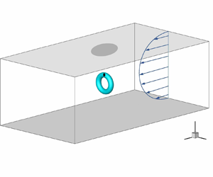
We investigate the influence of vortices remote from the boundary on the near-wall flow dynamics in wall-bounded flows. A vortex ring with precisely controlled local twist is introduced into the outer layer of a channel flow at a moderate Reynolds number. We find that the minimum vorticity flux for triggering the transition to turbulence is significantly reduced from the initial disturbance of an untwisted vortex ring to that of a twisted ring. In particular, the latter disturbance can cause vortex bursting in the early transitional stage. The impact of vortex bursting on the transition process is characterised by the near-wall, wall-normal velocity with the rapid distortion theory. The wall-normal velocity grows during vortex bursting, and leads to streak formation and then the transition to turbulence. The notable wall-normal velocity is induced by the large di-vorticity generated in vortex bursting. We model the growing radial component of the di-vorticity in terms of the local twist, and demonstrate that its surge is due to the generation of highly twisted vortex lines in vortex bursting. Then, we derive that the generation of the di-vorticity in the outer layer enhances the wall-normal velocity in the inner layer via the Poisson equation with the image method and the multipole expansion. Thus, we elucidate that the vortex bursting can have an effect on the transition process.

Type
JFM Papers
Copyright
© The Author(s), 2024. Published by Cambridge University Press

1. Introduction

Vortex dynamics has been extensively studied in various wall-bounded flows (Adrian Reference Adrian2007; Wu, Ma & Zhou Reference Wu, Ma and Zhou2007; Farrell & Ioannou Reference Farrell and Ioannou2012; He et al. Reference He, Wang, Pan, Feng, Gao and Rinoshika2017; Luckring Reference Luckring2019). In particular, the hairpin vortex, consisting of a ring-like head and quasi-streamwise legs, was observed in the transition and boundary-layer turbulence (Hussain Reference Hussain1986; Haidari & Smith Reference Haidari and Smith1994; Zhou, Adrian & Balachandar Reference Zhou, Adrian and Balachandar1996; Schoppa & Hussain Reference Schoppa and Hussain2002; Zhao, Yang & Chen Reference Zhao, Yang and Chen2016; Zhao et al. Reference Zhao, Xiong, Yang and Chen2018). However, the exact role of the vortex in the transition is still not clear. Since the vortex is usually generated from the mean shear, it is difficult to distinguish its contributions. In the present study, we introduce a vortex ring, the properties of which can be controlled precisely (Shen et al. Reference Shen, Yao, Hussain and Yang2023), into a channel flow, to elucidate its effect on the transition.

Different types of disturbances were introduced near the boundary to trigger transition to turbulence, e.g. the sinusoidal velocity disturbance (Brandt & Henningson Reference Brandt and Henningson2002), wake (Wu et al. Reference Wu, Jacobs, Hunt and Durbin1999), puff (Rubin, Wygnanski & Haritonidis Reference Rubin, Wygnanski and Haritonidis1980; Peixinho & Mullin Reference Peixinho and Mullin2006), free-stream turbulence (Jacobs & Durbin Reference Jacobs and Durbin2001; Fransson, Matsubara & Alfredsson Reference Fransson, Matsubara and Alfredsson2005) and various disturbances generated in experiments (Hof, Juel & Mullin Reference Hof, Juel and Mullin2003; Mullin Reference Mullin2011). Most of these methods introduce the disturbance directly into the near-wall region. However, in many transition scenarios, we only know the condition in the outer layer (with the wall unit larger than 50). For instance, the turbine blade is influenced by the vortex detached from the preceding blade. Therefore, understanding how the external vortex disturbances penetrate into the boundary (Hunt & Durbin Reference Hunt and Durbin1999) and their induction effect near the boundary remains an open problem.

The mechanisms of the induction and penetration of external vortices jointly introduce near-wall disturbances to trigger transition (Hunt & Durbin Reference Hunt and Durbin1999; Zaki & Durbin Reference Zaki and Durbin2005). In the receptivity stage, external disturbances, e.g. sound waves or turbulence, stimulate instability waves within the boundary layer (Saric, Reed & Kerschen Reference Saric, Reed and Kerschen2002; Zhong & Wang Reference Zhong and Wang2012). Subsequently, the instability of streaks (Ricco, Luo & Wu Reference Ricco, Luo and Wu2011; Wu Reference Wu2019; Xu et al. Reference Xu, Liu, Zhang and Wu2023), Tollmien–Schlichting (TS) waves (Sandham & Kleiser Reference Sandham and Kleiser1992; Schlatter, Stolz & Kleiser Reference Schlatter, Stolz and Kleiser2004) and $\varLambda$- and hairpin-like vortices (Sandham & Kleiser Reference Sandham and Kleiser1992; Zhao et al. Reference Zhao, Yang and Chen2016) promote the transition process. Finally, the emergence of turbulent spots (Wu Reference Wu2023) signals the onset of turbulence.

Distinguished from the current methods of introducing external disturbances, we employ a controllable vortex ring to induce transition. The vortex ring has been widely used as an elemental vortical structure to understand various vortical flows (Saffman Reference Saffman1981; Shariff & Leonard Reference Shariff and Leonard1992; Olsthoorn & Dalziel Reference Olsthoorn and Dalziel2015). The instability (Dazin, Dupont & Stanislas Reference Dazin, Dupont and Stanislas2006), dissipation (Archer, Thomas & Coleman Reference Archer, Thomas and Coleman2008) and axial-flow effect (Cheng, Lou & Lim Reference Cheng, Lou and Lim2010) of the vortex ring have been studied. However, these studies on the vortex ring are limited to the free domain without boundary conditions.

By extending the paradigm of vortex dynamics to wall flows, we analytically construct various vortex rings in the outer layer of a channel flow using the method in Shen et al. (Reference Shen, Yao, Hussain and Yang2023). The construction method can precisely adjust the vorticity flux and local twist, enabling us to examine the effect of various vortex-ring properties on the transition. In particular, we construct a vortex ring with opposite chiralities to mimic the hairpin-vortex head consisting of twisted vortex lines. The collision of twist vortex waves in this vortex ring causes vortex bursting (Melander & Hussain Reference Melander and Hussain1994; Arendt, Fritts & Andreassen Reference Arendt, Fritts and Andreassen1997; Cuypers, Maurel & Petitjeans Reference Cuypers, Maurel and Petitjeans2003; Ji & Van Rees Reference Ji and Van Rees2022; Shen et al. Reference Shen, Yao, Hussain and Yang2023), which can have an effect on the transition process. Furthermore, studying the vortical disturbance from the outer layer can be of importance in the control of transition.

The outline of this paper is organised as follows. Section 2 provides an overview of the initial flow set-up and numerical method. Section 3 discusses the important stages in the vortex-ring-induced transition, and characterises the effect of vortex evolution on the transition using the wall-normal velocity. Section 4 introduces the di-vorticity to explain the induction effect of the vortex ring on the wall-normal velocity. Conclusions are drawn in § 5.

2. Flow set-up and numerical overview

2.1. Initial flow set-up

The direct numerical simulation (DNS) is performed in a three-dimensional (3-D) channel domain ${\mathcal {V}}$ with coordinates ${\boldsymbol {x}}=(x,y,z)\in {\mathcal {V}}$ and in the streamwise $x$-, the wall-normal $y$- and spanwise $z$-directions, respectively. The streamwise length of the channel is $L_x=5.61$, wall-normal height is $L_y=2 H$ with $H =1$ and spanwise width is $L_z=2.99$, consistent with those in the DNS in Zhao et al. (Reference Zhao, Yang and Chen2016). The dimensionless 3-D incompressible Navier–Stokes (NS) equations of the velocity ${\boldsymbol {u}}=(u,v,w)$ scaled by $H$ and the bulk velocity $U_b$ read

(2.1)\begin{equation} \left.\begin{gathered} \frac{\partial {\boldsymbol{u}}}{\partial t}+{\boldsymbol{u}} \boldsymbol{\cdot} \boldsymbol{\nabla} {\boldsymbol{u}}={-}\boldsymbol{\nabla} p+ \frac{1}{{{\it Re}}} \nabla^2 {\boldsymbol{u}}+{\boldsymbol{f}},\\ \boldsymbol{\nabla} \boldsymbol{\cdot} {\boldsymbol{u}}=0, \end{gathered}\right\} \end{equation}

where $t$ denotes the time, $p$ the pressure, $\nu$ the kinematic viscosity and ${{\it Re}}={U_b H}/{\nu }$ the Reynolds number. The flow is driven by a constant flux rate with $U_b= 1$ by exerting a homogeneous time-dependent body force ${\boldsymbol {f}}=(\tau _w,0,0)$, where

(2.2)\begin{equation} \tau_w\equiv\frac{1}{{\it Re}}{\frac{\mathrm{d} \langle u\rangle}{\mathrm{d} y}} \end{equation}

denotes the wall shear stress and $\langle {\cdot }\rangle$ the volume average.

As sketched in figure 1(a), periodic boundary conditions are applied in $x$- and $z$-directions, and the no-slip boundary conditions are applied at the upper boundary $y = -1$ and lower boundary $y = 1$. The initial flow field contains a vortex ring embedded in the laminar Poiseuille flow. The vortex ring serves as a controllable initial disturbance to trigger transition. The Poiseuille base flow has a velocity profile

(2.3)\begin{equation} u_l=U_0(1-y^2) \end{equation}

with the centreline velocity $U_0=1.5$. If not otherwise specified, the Reynolds number is set as ${{\it Re}}= 3333$ (Kim, Moin & Moser Reference Kim, Moin and Moser1987). If the flow undergoes a transition, this ${\it Re}$ is equivalent to the friction Reynolds number ${\it Re}_\tau ={\it Re} \sqrt {\tau _w}=207$, where $\tau _w$ is obtained in the fully developed turbulent stage. The vorticity ${\boldsymbol {\omega }} = \boldsymbol {\nabla } \times {\boldsymbol {u}}$ of the base flow only has a spanwise component

(2.4)\begin{equation} \omega_l=3y. \end{equation}

Figure 1. (a) Schematic of the initial flow set-up for the vortex-ring-induced transition. The grey plane denotes the solid-wall boundary of the channel flow. The vortex ring (light blue surface) is placed at the centre of the computation domain. The possible vortex bursting is located at $(x_{br},y_{br},z_{br})$, and it has a strong induction effect near the upper boundary (marked by dark grey patch). (b) Schematic of the vortex ring. The dash-dotted line denotes the centreline $\mathcal {C}$ of the vortex tube (light blue surface), and the red line denotes a typical twisted vortex line attached on the vortex tube. Local cylindrical coordinates $(s,\rho,\theta )$ inside the vortex tube are marked in a cross section.

The vortex ring, represented by the light blue surface in figure 1(a), is placed at the centre of the computation domain, the farthest position from the wall. Note that the vortex ring can be placed anywhere in the outer layer. In general, the induction effect of the vortex ring on flow transition grows with the initial distance between the vortex-ring centre and the nearest wall.

The embedded vortex ring is set up using the method in Shen et al. (Reference Shen, Yao, Hussain and Yang2023). The geometry of vortex lines attached on the vortex tube is sketched in figure 1(b). The vorticity of the vortex ring is specified as

(2.5)\begin{equation} {\boldsymbol{\omega}}(s,\rho,\theta)=\varGamma f(\rho) \left(\frac{\rho\eta}{1-\kappa \rho \mathrm{cos}\theta}{\boldsymbol{e}}_{\theta}+{\boldsymbol{e}}_{s}\right), \end{equation}

where $(s,\rho,\theta )$ are curved cylindrical coordinates, $({\boldsymbol {e}}_{s},{\boldsymbol {e}}_{\rho },{\boldsymbol {e}}_{\theta })$ denote axial, radial and azimuthal basis, respectively, $\kappa$ is the constant curvature of the centreline $\mathcal {C}$ of the vortex ring, $\varGamma$ is the vorticity flux of the vortex ring and $f(\rho )=\exp (-{\rho ^2}/{2 \sigma ^2})/({2 {\rm \pi}\sigma ^2})$ is a Gaussian function parameterised by the standard deviation $\sigma$. Moreover, the local twist rate $\eta$ measures the twisting number of vortex lines along the vortex centreline inside the vortex ring.

In the numerical construction, ${\boldsymbol {\omega }}(s,\rho,\theta )$ in (2.5) in curved cylindrical coordinates is mapped to ${\boldsymbol {\omega }}(x, y, z)$ in Cartesian coordinates using the algorithm in appendix A of Shen et al. (Reference Shen, Yao, Hussain and Yang2023). Various closed vortex tubes (Shen et al. Reference Shen, Yao, Hussain and Yang2022) can be constructed with a given parametric equation for the centreline and the function $f(\rho )$ for the vorticity-flux distribution.

2.2. Internal structures of the vortex ring

The configuration parameters of the vortex ring are set based on the DNS result of the same channel flow in Zhao et al. (Reference Zhao, Yang and Chen2016). As illustrated by the isosurface of the swirling strength $\lambda _{ci}$ (Zhou et al. Reference Zhou, Adrian, Balachandar and Kendall1999) in figure 2, the head of the hairpin-like vortex tube forms a ring-like structure consisting of helical vortex lines in the late stage of the natural transition. In particular, the twist rate of vortex lines is not uniformly distributed on the vortex ring. The chiralities of the helical lines are opposite on the two halves of the ring.

Figure 2. Modelling an external vortex in flow transition using a vortex ring. (a) Isosurface of the swirling strength $\lambda _{ci}=2$ (Zhou et al. Reference Zhou, Adrian, Balachandar and Kendall1999) at $t =110$ in the late stage of the natural transition in channel flow reported in Zhao et al. (Reference Zhao, Yang and Chen2016). The isosurface is colour-coded by the helicity density $h={\boldsymbol {\omega }}\boldsymbol {\cdot }{\boldsymbol {u}}$. The hairpin head consisting of helical vortex lines is sketched in the closed-up view on the left. The orange arrows denote axial flows inside the vortex tube induced by the helical vortex lines with opposite chiralities. (b) Isosurface of the $\lambda _{ci}=2$ (colour-coded by $h$) in the present vortex-ring-induced transition. The helical vortex lines with opposite chiralities near the vortex ring are plotted in the closed-up view on the left. The possible bursting location is marked by the asterisk at $s={\rm \pi} R/2$ in the local cylindrical coordinates.

Thus, we set the differential twist, i.e. the non-uniform local twist rate $\eta =A\cos (s/R)$ along $\mathcal {C}$, with the constant $A=120$ (Shen et al. Reference Shen, Yao, Hussain and Yang2023). For comparison, we also set cases with the uniform twist $\eta =2A/{\rm \pi}$ and zero twist $\eta =0$. The initial twist is crucial in determining whether the vortex ring will burst during its evolution (Shen et al. Reference Shen, Yao, Hussain and Yang2023). In addition, the vorticity flux $\varGamma$, vortex ring radius $R = 0.25$ and ring thickness $\sigma = 0.0125$ are comparable to the DNS result in Zhao et al. (Reference Zhao, Yang and Chen2016) at $t=110$ in the late transition. Note that the induction effect of the vortex ring on flow transition strongly depends on $A$, which plays a similar role as ${\it Re}$, whereas it weakly depends on $R$ and $\sigma$ (Shen et al. Reference Shen, Yao, Hussain and Yang2022Reference Shen, Yao, Hussain and Yang2023).

2.3. DNS

The NS equations (2.1) are solved by DNS using the same spectral method in Kim et al. (Reference Kim, Moin and Moser1987). The velocity in the $x$- and $z$-directions is decomposed into Fourier modes, and ${\boldsymbol {u}}$ in the $y$-direction is solved by the Helmholtz equations for each mode. The time stepping is varied to ensure the Courant–Friedrichs–Lewy number less than $0.6$. The initial vorticity field, the superposition of laminar background (2.4) and vortex ring (2.5), is decomposed into Fourier–Chebyshev modes. To satisfy the boundary conditions for a channel, the initial velocity field is calculated from the vorticity via the Helmholtz equation in the Fourier–Chebyshev space. A boundary correction is then applied under the divergence-free constraint, which is detailed in Appendix A. In the calculation of flow evolution, the two-thirds truncation method is applied for dealiasing (Canuto et al. Reference Canuto, Hussaini, Quarteroni and Zang1988). The low-storage third-order semi-implicit Runge–Kutta method (Philippe, Robert & Michael Reference Philippe, Robert and Michael1991; Yang & Pullin Reference Yang and Pullin2011) is used for time marching.

We performed convergence tests on four grids with $N_x\times N_y\times N_z =768\times 769 \times 768$, $576\times 577 \times 576$, $384\times 385 \times 384$ and $192\times 193 \times 192$ grid points. After examining the convergence of the maximal vorticity magnitude for vortex evolution at $t\leqslant 1.5$ and ${\it Re}_\tau$ for flow transition at $t\leqslant 70$, we chose the grid of $384\times 385 \times 384$ for the simulation at ${\it Re} = 3333$. We conducted an additional DNS at ${\it Re}=8090$ on the grid of $768\times 769 \times 768$ to study the effect of ${\it Re}$.

3. Transition induced by a vortex ring

3.1. Stages in transition process

In this section, we demonstrate that the initially embedded vortex ring can induce transition in wall flows at moderate ${\it Re}$, and the critical magnitude of the initial disturbance is highly dependent on the initial twist of the vortex ring. For the vortex rings with three different $\eta$, we first examine the critical vorticity flux $\varGamma = \varGamma ^*$ to induce transition. Here, $\varGamma ^*$ is determined by assessing whether the flow will undergo a transition through a series of simulations conducted for various values of $\varGamma$.

As listed in table 1, we set up four DNS cases for the vortex-ring-induced transition to illustrate the influence of the internal structure inside the vortex ring. In Case 1, the initial vortex ring with chirality-opposite helical structures mimics the hairpin head in the natural transition, and it has the minimum $\varGamma ^*$. As shown in figure 2, the isosurface of $\lambda _{ci}$ colour-coded by the helicity density $h={\boldsymbol {u}}\boldsymbol {\cdot }{\boldsymbol {\omega }}$ shows positive and negative $h$ in the two halves of the vortex ring. In this case, we set $\varGamma \approx 1.2 \varGamma ^*$ to quickly trigger transition.

Table 1. Parameters $\eta$ and $\varGamma$ of the vortex ring in four representative cases of the vortex-ring-induced transition of channel flow. The threshold vorticity flux $\varGamma ^*$ for triggering transition, $\varGamma ^*$ normalised by $\varGamma ^*_{\eta =0}$ ($\varGamma ^*$ in Case 4) and the volume-averaged disturbance energy $E_t$ are listed. Note that Cases 1, 3 and 4 have the transition with $\varGamma \approx 1.2 \varGamma ^*$.

In Case 2, the vortex ring is the same except that the twist is uniform, and $\varGamma ^*$ is more than twice of that in Case 1. Thus, Case 2 has no transition with $\varGamma < \varGamma ^*$. Note that Cases 1 and 2 have roughly the same disturbance energy

(3.1) \begin{equation} E_t=\frac{1}{V}\int_{\mathcal{V}}\frac12((u-u_l)^2+v^2+w^2)\,\mathrm{d} {\mathcal{V}}, \end{equation}

where $V$ denotes the volume of the channel. Therefore, the different twist distributions in Cases 1 and 2 only have a minor effect on $E_t$, but they have an effect on the transition process. Case 3 is the same as Case 2 except $\varGamma > \varGamma ^*$, so it has transition. In Case 4, the vortex ring with $\eta = 0$ and $\varGamma > \varGamma ^*$ also induces transition.

The evolution of ${{\it Re}}_\tau$, indicating the variation of the wall friction, in the four cases is plotted in figure 3. It can be roughly divided into three stages. Before a characteristic time $t_1=1$, the major dynamics is only within the vortex ring, including the vortex bursting in Case 1. From $t_1$ to $t_2 = 10$, the vortex ring breaks up, and ${{\it Re}}_\tau$ grows mildly. From $t_2$ to $t_3 = 40$, ${{\it Re}}_\tau$ starts to surge and the transition occurs in the cases with $\varGamma > \varGamma ^*$, whereas ${{\it Re}}_\tau$ remains at the laminar value for $\varGamma < \varGamma ^*$. The flow evolution in the three stages is elaborated on in the following.

Figure 3. Temporal evolution of the wall-friction Reynolds number in various cases (listed in table 1).

3.1.1. Stage 1: dynamics inside the vortex ring

Figure 4 shows the main dynamics inside the vortex ring around $t_1$. In Case 1, an initially helical vortex ring with differential twist has the azimuthal vorticity $\omega _\theta$, which generates the axial velocity

(3.2)\begin{equation} u_s(s, \rho, \theta)=\frac{1}{1-\kappa \rho \cos \theta} \frac{\varGamma }{2{\rm \pi}}\exp\left(-\frac{\rho^2}{2\sigma^2}\right)\eta \end{equation}

along the vortex-ring centreline (see Appendix B for a detailed derivation). The two twist vortex waves with opposite chiralities collide at the symmetrical plane at $s={{\rm \pi} R}/{2}$. This leads to vortex bursting (Shen et al. Reference Shen, Yao, Hussain and Yang2023): a part of the vortex tube is flattened on the symmetrical plane, forming a disc-like structure with highly spiral vortex lines.

Figure 4. Evolution of the isosurface of $\lambda _{ci}$ during the vortex bursting in Case 1 with two Reynolds numbers. The surface is colour-coded by the helicity density: (a) $t=0.3$ and $\lambda _{ci}=2.4$; (b) $t=0.9$ and $\lambda _{ci}=2.4$;(c) $t=1.5$ and $\lambda _{ci}=2.1$.

Using the vortex-ring model in Shen et al. (Reference Shen, Yao, Hussain and Yang2023), the starting and ending times of the vortex bursting in Case 1 are defined as

(3.3)\begin{equation} t_{bs}=\frac{2 {\rm \pi}R}{\varGamma A }\approx 0.3 \end{equation}

and

(3.4)\begin{equation} t_{be}=\frac{ 10 {\rm \pi}^2 R}{3 \varGamma A }\approx 1.5, \end{equation}

respectively. Figure 4(a,c) shows the vortical structures at $t_{bs}$ and $t_{be}$.

Moreover, the vortices for ${\it Re}=3333$ and 8090 are nearly identical in figure 4(a), because the viscosity dependence is weak at early times, consistent with the model in (3.2). In figure 4(c), the ${\it Re}$-effect becomes noticeable because the model in (3.2) breaks down near the bursting site with strong viscous vortex reconnection. As discussed in Shen et al. (Reference Shen, Yao, Hussain and Yang2023), increasing ${\it Re}$ is equivalent to increasing an effective $\eta$. A larger $\eta$ in (3.2) suggests a larger $u_s$, leading to stronger vortex bursting with generating larger disc-like structures. By contrast, there is no bursting in Cases 2–4 for initial vortex rings with uniform or zero twist.

3.1.2. Stage 2: breakup of the vortex ring

Figure 5(ac) illustrate the breakup dynamics of the vortex ring from $t_1$ to $t_2$ in Cases 1–3, respectively. At $t=t_1$, the initially helical vortex ring splits into primary and secondary rings due to the axial flow (Cheng et al. Reference Cheng, Lou and Lim2010). The primary vortex ring undergoes further transition, and the secondary rings dissipate before $t_2$. By contrast, the vortex with $\eta =0$ in Case 4 retains its ring shape at $t=t_1$ in figure 5(d).

Figure 5. Evolution of the isosurface of $\lambda _{ci}$ in the second stage of transition in (a) Case 1 with $\eta =A\cos {\xi }$ and $\varGamma =0.047$, (b) Case 2 with $\eta =2A/{\rm \pi}$ and $\varGamma =0.047$, (c) Case 3 with $\eta =2A/{\rm \pi}$ and $\varGamma =0.097$ and(d) Case 4 with $\eta =0$ and $\varGamma =0.278$. The isocontour values in each row are $\lambda _{ci}=2.1$ at $t=1$ and $\lambda _{ci}=1$ at $t=5$ and 9. The isosurface is colour-coded by the helicity density. The blue arrows in (a) denote the direction of the mean flow. Black lines denote vortex lines.

From $t_1$ to $t_2$, the vortex rings with and without the initial twist evolve very differently. For $\eta >0$, the vortex rings experience dramatic deformation in figure 5(ac). The uniformly twisted vortex ring folds and elongates under the mean shear in figure 5(b,c). This process from $t=1$ to $t=5$ in Case 2 is further illustrated in the side view in figure 6. The vortex ring is persistently stretched along the streamwise direction until $t=9$, and eventually breaks up into several pairs of streamwise vortices. Although the evolutions of the vortices are similar in Cases 2 and 3, the larger $\varGamma$ in Case 3 induces a transition whereas the flow relaminarises in Case 2. The ring with differential twist has a similar evolution in figure 5(a). Since its internal structure is already unstable at $t=t_1$, the breakup process in Case 1 is faster than in Cases 2 and 3, which agrees with the different growth rates of ${{\it Re}}_\tau$ in figure 3.

Figure 6. Evolution of the isosurface of $\lambda _{ci}$ from $t=1$ to $t=5$ in Case 2 with $\eta =2A/{\rm \pi}$ and $\varGamma =0.047$ (side view). The isosurface is colour-coded by the helicity density.

The vortex ring with $\eta = 0$ does not break up in stage 2. Its aspect ratio oscillates in figure 5(d) due to the elliptic instability (Kerswell Reference Kerswell2002) with the ring deformation in the $x$-direction and the curvature instability (Fukumoto & Hattori Reference Fukumoto and Hattori2005; Blanco-Rodríguez & Dizès Reference Blanco-Rodríguez and Dizès2017) with the variation of the ring curvature.

3.1.3. Stage 3: late transition

Cases 1–3 at $t_3$ in stage 3 of late transition are very similar. In figure 7 for Case 1, the inverse hairpin-like structure in figure 7(a) evolves into streamwise vortices in figure 7(b), which characterise a quasi-stable TS wave (Boiko et al. Reference Boiko, Westin, Klingmann, Kozlov and Alfredsson1994). Then the flow evolves as in the natural transition (Zaki Reference Zaki2013; Zhao et al. Reference Zhao, Yang and Chen2016), i.e. from streaks to the $\varLambda$- or hairpin-like structure in figure 7(c), and finally it breaks down into turbulence in figure 7(d). Moreover, the transition follows an almost identical route at a larger ${\it Re}=8090$, whereas the rise of ${\it Re}_\tau$ occurs much earlier than that at ${\it Re}=3333$ (not shown).

Figure 7. Evolution of the isosurface of $\lambda _{ci}$ after the dissipation of the vortex ring in Case 1. The surface is colour-coded by the wall distance. Note that the channel is flipped in the $y$-direction for clearly showing the vortical structure: (a) $t=10$ and $\lambda _{ci}=1.3$; (b) $t=20$ and $\lambda _{ci}=0.5$; (c) $t=30$ and $\lambda _{ci}=1$; (d) $t=40$ and $\lambda _{ci}=1.3$.

In particular, the evolution and generation of the hairpin vortices are depicted in figure 8. The signature of hairpin vortices aligns with that in Adrian, Meinhart & Tomkins (Reference Adrian, Meinhart and Tomkins2000) in terms of the streamwise length, wall-normal location and angle between hairpin head and neck. From $t=31$ to $t=34$, the primary hairpin vortex elongates streamwise, and the secondary hairpin vortex forms at the ridge of the primary one (Zhou et al. Reference Zhou, Adrian, Balachandar and Kendall1999). Then, more hairpin-like structures emerge at the ridges of the primary and secondary hairpins at $t=35$, forming a coherent packet of hairpins. These observations are consistent with the auto-generation mechanism (Zhou et al. Reference Zhou, Adrian, Balachandar and Kendall1999; Adrian Reference Adrian2007; Kim et al. Reference Kim, Adrian, Balachandar and Sureshkumar2008).

Figure 8. Evolution of the isosurface of $\lambda _{ci}=1$ during the generation and evolution of hairpin vortices in Case 1. The isosurface is colour-coded by the helicity density. Note that the channel is flipped in the $y$-direction for clearly showing the vortical structure.

Note that the route of late transition induced by the vortex ring with large vorticity flux and zero-twist in Case 4 is distinguished from the others induced by the twisted vortex ring. The initial vortex ring gradually dissipates and disappears in Case 4, without forming any other vortical structures at $t=10$ in figure 9(a). It evolves into streamwise vortices near the outer layer at very late times in figure 9(b,c) and finally breaks down into turbulence in figure 9(d).

Figure 9. Evolution of the isosurface of $\lambda _{ci}$ in Case 4: (a) $t=10$ and $\lambda _{ci}=1$; (b) $t=20$ and $\lambda _{ci}=0.7$;(c) $t=30$ and $\lambda _{ci}=0.5$; (d) $t=50$ and $\lambda _{ci}=2$. The surface is colour-coded by the wall distance.

3.2. Transition induced by vortex bursting

The internal dynamics of the vortex ring around $t_1= 1$ is much faster than the disturbance growth in the boundary layer around $t_3=40$, so these two processes can be decoupled. The initial amplitude of the disturbance is determined by the dynamics of the vortex ring before $t_1$, whereas the subsequent linear amplification mechanism is mainly influenced by the background shear.

According to the rapid distortion theory (Sreenivasan & Narasimha Reference Sreenivasan and Narasimha1978; Savill Reference Savill1987; Nazarenko, Kevlahan & Dubrulle Reference Nazarenko, Kevlahan and Dubrulle1999; Deissler Reference Deissler2004), the amplitude of the disturbance is low in the early stage of transition, so the disturbance growth can be treated as inviscid. Moffatt (Reference Moffatt1967) applied the rapid distortion theory to the viscous sublayer (Saric et al. Reference Saric, Reed and Kerschen2002) at $y^+<5$, where

(3.5)\begin{equation} y^+={(1-y)}{\it Re}_\tau \end{equation}

is the normalised distance from the upper wall at $y=1$, and the wall-normal length scale is much smaller than the streamwise one.

We consider the near-wall velocity ${\boldsymbol {u}}_B=(u_B,v_B,w_B)$ with

(3.6ac)\begin{equation} u_B=u(x,y^+,z),\quad v_B=v(x,y^+,z),\quad w_B=w(x,y^+,z),\quad y^+ < 5. \end{equation}

Moffatt (Reference Moffatt1967) showed that when the disturbance amplitude is small, the streamwise disturbance mode $\hat {u}_B$ grows linearly with the wall-normal disturbance mode $\hat {v}_B$ as

(3.7)\begin{equation} \hat{u}_B(k_x,k_z)=\hat{u}_{B0}(k_x,k_z)-\mathcal{S}\hat{v}_B(k_x,k_z) t, \end{equation}

where $\hat {\cdot }$ denotes the Fourier transform of a quantity in the $x$$z$ plane with wavenumbers $k_x$ and $k_z$, subscript $0$ denotes the initial value and $\mathcal {S}= -2U_0y$ is the shear rate of the Poiseuille flow. From (3.7), $\hat {v}_B$ is determined by the state around $t=t_1$, $\mathcal {S}$ is constant for a given $y$ and $\hat {u}_B$ depends on $\hat {v}_B$, e.g. $\hat {u}_B$ increases with $t$ for positive $-\mathcal {S}\hat {v}_B$.

We examine the evolution of $\hat {v}_B(k_{xz},y^+)$ during the period of vortex bursting from $t_{bs}$ to $t_{be}$, with $k_{xz}=\sqrt {k_x^2+k_z^2}$. Based on the Parseval identity, we use

(3.8)\begin{equation} \overline{v_B^2}(y^+)=\frac{1}{A_{xz}}\iint v_B^2({x,y^+,z})\,\mathrm{d}\kern1pt x\,\mathrm{d} z = \sum_{k_{xz}}\hat{v}_B^2(k_{xz},y^+) \end{equation}

to quantify the averaged amplitude of $\hat {v}_B$, where $A_{xz}$ denotes the area of the $x$$z$ plane. Figure 10 plots the evolution of $\overline {v_B^2}(y^+=1)$ in Cases 1–3 in the very early stage when (3.7) is valid. Note that the evolution of $\overline {v_B^2}(y^+=5)$ is qualitatively the same (not shown). Case 2 has the lowest amplitude, and it has no transition. Cases 1 and 3 have larger amplitudes, suggesting the higher disturbance growth rate from (3.7), and both cases have transition. At early times, $\overline {v_B^2}(y^+=1)$ decays in Cases 2 and 3 due to the viscous effect, and its decay rate depends on the initial $\varGamma$. By contrast, $\overline {v_B^2}(y^+=1)$ grows by 15 % from $t_{bs}$ to $t_{be}$ in Case 1. The growth of $v_B$ during the vortex bursting will be further discussed in § 4.

Figure 10. Evolution of $\overline {v_B^2}(y^+=1)$, as metric for the averaged amplitude of $\hat {v}_B(k_{xz},y^+=1)$, from $t_{bs}$ to $t_{be}$ during the vortex bursting in Cases 1–3.

The transition is induced by the growth of $v_B$. According to (3.7), the streamwise disturbance of $u_B$ grows with the vortex-ring induced $v_B$ (Landahl Reference Landahl1975Reference Landahl1980). The streaks are lifted by $v_B$ in figure 7(a) and then elongated by the mean shear in figure 7(b), resulting in streamwise streaks downstream (Brandt & Henningson Reference Brandt and Henningson2002). A hairpin vortex (Zhou et al. Reference Zhou, Adrian, Balachandar and Kendall1999) emerges from the streaks in figure 7(c), and then it evolves into a hairpin packet by the auto-generation mechanism (Adrian et al. Reference Adrian, Meinhart and Tomkins2000; Adrian Reference Adrian2007; Kim et al. Reference Kim, Adrian, Balachandar and Sureshkumar2008). The vortices break down and form a turbulent spot in figure 7(d), which eventually leads to a fully developed turbulent state (Wu Reference Wu2023).

In summary, the threshold vorticity flux $\varGamma ^*$ is reduced from $0.231$ in Case $4$ to $0.0394$ in Case $1$ (see table 1) due to the induction of $v_B$ in the vortex-ring evolution. In particular, the vortex bursting in Case 1 produces strong $v_{B}$ near the boundary, enhancing the growth of $u_B$ and then triggering a transition.

4. Induction of the wall-normal velocity in vortex bursting

4.1. Introduction of the di-vorticity

Next we elucidate the induction mechanism of $v_B$ in the near-wall region by the large di-vorticity generated in the outer layer during the vortex bursting. The di-vorticity ${{\boldsymbol {\varrho }}}=\boldsymbol {\nabla }\times {\boldsymbol {\omega }}$ measures the local rotational intensity of the vorticity, and large ${{\boldsymbol {\varrho }}}$ may correspond to the local helical geometry of vortex lines. The identity $\nabla ^2 {\boldsymbol {u}}=\boldsymbol {\nabla }(\boldsymbol {\nabla }\boldsymbol {\cdot }{\boldsymbol {u}})-{\boldsymbol {\varrho }}$ suggests the Poisson equation

(4.1)\begin{equation} \nabla^2 {\boldsymbol{u}}={-}{\boldsymbol{\varrho}} \end{equation}

for the incompressible flow.

The di-vorticity has a very intermittent distribution in the transition. In Case 1, the maximum $| {\boldsymbol {\varrho }}|$ can be hundreds of times the volume-averaged $| {\boldsymbol {\varrho }}|$ during the vortex bursting. For example, at $t=0.9$ in Case 1, the region with $| {\boldsymbol {\varrho }}| \geqslant 1000$ enclosed by the isosurface of $| {\boldsymbol {\varrho }}|=1000$ occupies only $0.2\,\%$ of the volume of the entire channel in figure 11(a), but ${\boldsymbol {\varrho }}$ in this negligibly small region can reconstruct the vortical structure very close to the original in figure 11(b). Therefore, the highly concentrated ${\boldsymbol {\varrho }}$ near the site of vortex bursting can drive the near-wall flow dynamics in a finite time period after vortex bursting.

Figure 11. Reconstruction of the flow field using a small potion of the di-vorticity in Case 1 at $t=0.9$.(a) Isosurface of $\lambda _{ci}=2$ (blue) in the DNS, and isosurface of $| {\boldsymbol {\varrho }}|=1000$ (red). (b) Isosurface of $\lambda _{ci}=2$ in the flow field reconstructed from the di-vorticity in the region enclosed by the isosurface of $| {\boldsymbol {\varrho }}|=1000$ (red surface in (a)). Note that this subdomain occupies only $0.2\,\%$ of $V$.

With higher-order velocity derivatives, ${\boldsymbol {\varrho }}$ has conservation constraints under given boundary conditions. The solid-wall boundary conditions are

(4.2)\begin{equation} \left.\begin{gathered} {\boldsymbol{u}}=0,\quad {\boldsymbol{u}}\in{\partial}{\mathcal{V}},\\ \frac{{\partial} v}{{\partial} y} = 0,\quad v\in{\partial}{\mathcal{V}}, \end{gathered}\right\} \end{equation}

which imposes the constraint

(4.3)\begin{equation} \int_{\mathcal{V}}y^n\varrho_y\mathrm{d} {\mathcal{V}}=0,\quad n\in\mathbb{N} \end{equation}

on the di-vorticity. This constraint implies that the wall can have a response near the boundary to counter ${\boldsymbol {\varrho }}$ generated in a vortex-dynamics event remote from the wall. For $n=0$, (4.3) suggests that the flow evolution only redistributes $\varrho _y$ rather than changing the volume integration of $\varrho _y$. The implication of (4.3) will be further discussed in § 4.3.

4.2. Generation of the di-vorticity during vortex bursting

We demonstrate that large ${\boldsymbol {\varrho }}$ can be generated during the bursting of a vortex ring. The governing equation of ${\boldsymbol {\varrho }}$ is

(4.4)\begin{equation} \frac{\mathrm{D} {\boldsymbol{\varrho}}}{\mathrm{D} t}=\boldsymbol{\nabla}\times\boldsymbol{\nabla}\times{\boldsymbol{a}}+{\boldsymbol{\omega}}\boldsymbol{\cdot}\boldsymbol{\nabla}{\boldsymbol{\omega}}+{\boldsymbol{L}}, \end{equation}

where ${\boldsymbol {a}} = -\boldsymbol {\nabla } p+\nabla ^2 {\boldsymbol {u}}/{\it Re}$ denotes the acceleration of a fluid particle, and

(4.5)\begin{equation} {\boldsymbol{L}}\equiv(\boldsymbol{\nabla}{\boldsymbol{\omega}}\boldsymbol{\cdot}\boldsymbol{\nabla}{\boldsymbol{u}}-\boldsymbol{\nabla}{\boldsymbol{u}}\boldsymbol{\cdot}\boldsymbol{\nabla}{\boldsymbol{\omega}}):{\boldsymbol{\varepsilon}} \end{equation}

has a form similar to the Lamb vector ${\boldsymbol {\omega }}\times {\boldsymbol {u}}$, with the Levi–Civita symbol ${\boldsymbol {\varepsilon }}$. On the right-hand side, the term $\boldsymbol {\nabla }\times \boldsymbol {\nabla }\times {\boldsymbol {a}}$ for the viscous effect can be neglected for very large ${\it Re}$, and then ${\boldsymbol {\omega }}\boldsymbol {\cdot }\boldsymbol {\nabla }{\boldsymbol {\omega }}$ and ${\boldsymbol {L}}$ dominate the evolution of ${\boldsymbol {\varrho }}$.

Given the initial vortex ring in (2.5), the evolution of ${\boldsymbol {\varrho }}$ is estimated in curved cylindrical coordinates $(s,\rho,\theta )$. The vorticity-stretching and Lamb-like terms become (see Appendix B for a detailed derivation)

(4.6)\begin{equation} {\boldsymbol{\omega}}\boldsymbol{\cdot}\boldsymbol{\nabla}{\boldsymbol{\omega}}=\left(0,0,\omega_s \frac{1}{h_s} \frac{{\partial} \omega_\theta}{{\partial} s} + \omega_\theta \frac{1}{\rho} \frac{{\partial} \omega_\theta}{{\partial} \theta}\right) \end{equation}

and

(4.7)\begin{equation} \left.\begin{gathered} {\boldsymbol{L}}=\left(\frac{1}{\rho}\frac{{\partial} \omega_\theta}{{\partial} \rho} \frac{{\partial} u_\theta}{{\partial} \theta}-\frac{1}{h_s}\frac{{\partial} u_s}{{\partial} \rho} \frac{{\partial} \omega_\theta}{{\partial} s}-\frac{1}{\rho}\frac{{\partial} u_\theta}{{\partial} \rho} \frac{{\partial} \omega_\theta}{{\partial} \theta}\right., \\ \frac{1}{\rho^2}\frac{{\partial} \omega_\theta}{{\partial} \theta}\frac{{\partial} u_s}{{\partial} \theta}- \frac{1}{h_s\rho}\frac{{\partial} \omega_\theta}{{\partial} s}\frac{{\partial} u_\theta}{{\partial} \theta}+ \frac{1}{h_s^2}\frac{{\partial} u_s}{{\partial} s}\frac{{\partial} \omega_\theta}{{\partial} s},\\ \left.-\frac{1}{h_s}\frac{{\partial} \omega_s}{{\partial} \rho}\frac{{\partial} u_s}{{\partial} s}- \frac{1}{\rho}\frac{{\partial} \omega_\theta}{{\partial} \rho}\frac{{\partial} u_s}{{\partial} \theta}\right), \end{gathered}\right\} \end{equation}

respectively, where $h_s=1-\kappa \rho \cos \theta$ is the Lamé coefficient in the $s$-direction.

We analyse the variation of ${\boldsymbol {\varrho }}$ using (4.4) before $t_1$ when the vortex bursting occurs (see figure 4). In the model of $\eta$ for a bursting vortex ring (Shen et al. Reference Shen, Yao, Hussain and Yang2023), the initial twist distribution $\eta (s,t=0)=A\cos (s/R)$ evolves into

(4.8)\begin{equation} \eta(s,\rho,t)= A\cos\left(\frac{s-B(\rho)\eta(s,\rho,t) t}{R}\right) \end{equation}

with $A=120$ and $B={\varGamma }\exp (-{\rho ^2}/{2\sigma ^2})/(2{\rm \pi} h_s)$, and (4.8) can be solved numerically using the explicit Newton method. Substituting (2.5) and (B2) into (4.8), we find that

(4.9a,b)\begin{equation} \frac{{\partial} \omega_\theta}{{\partial} s}\sim \frac{{\partial} \eta}{{\partial} s}\quad \textrm{and}\quad \frac{{\partial} u_s}{{\partial} s}\sim \frac{{\partial} \eta}{{\partial} s} \end{equation}

are dominant terms, where $\sim$ denotes an estimate of the order of magnitude. Other derivatives of ${\boldsymbol {u}}$ and ${\boldsymbol {\omega }}$ only depend on the initial configuration and remain constant during vortex bursting. With $ {\partial } \eta / {\partial } s\gg {\partial } \eta / {\partial } \theta$ and $ {\partial } \eta / {\partial } s \gg {\partial } \eta / {\partial } \rho$, we rank the magnitude of terms in (4.6) and (4.7) by $ {\partial } \eta / {\partial } s$. By only keeping the dominant terms, (4.4) is approximated by

(4.10)\begin{equation} \frac{\mathrm{D} {\boldsymbol{\varrho}}}{\mathrm{D} t}\approx\frac{1}{h_s}\left(-\frac{{\partial} u_s}{{\partial} \rho} \frac{{\partial} \omega_\theta}{{\partial} s}, -\frac{1}{\rho}\frac{{\partial} \omega_\theta}{{\partial} s} \frac{{\partial} u_\theta}{{\partial} \theta}+\frac{1}{h_s}\frac{{\partial} u_s}{{\partial} s} \frac{{\partial} \omega_\theta}{{\partial} s},\omega_s \frac{{\partial} \omega_\theta}{{\partial} s}- \frac{{\partial} \omega_s}{{\partial} \rho}\frac{{\partial} u_s}{{\partial} s}\right). \end{equation}

Here, the most influential term

(4.11)\begin{equation} I=\frac{1}{h_s^2}\frac{{\partial} u_s}{{\partial} s}\frac{{\partial} \omega_\theta}{{\partial} s}\sim \left(\frac{{\partial} \eta}{{\partial} s}\right)^2 \end{equation}

contains the product of two dominant terms. Finally, substituting (4.8) into (4.11), we estimate the order of (4.4) in terms of $\eta$ as

(4.12)\begin{equation} \frac{\mathrm{D} {\boldsymbol{\varrho}}}{\mathrm{D} t}\approx I{\boldsymbol{e}}_{\rho}\sim \left(\frac{{\partial} \eta}{{\partial} s}\right)^2 {\boldsymbol{e}}_{\rho}. \end{equation}

In figure 12, the distribution of $({ {\partial } \eta }/{ {\partial } s})^2$ along the $s$-direction shows that large $| {\boldsymbol {\varrho }}|$ is generated during vortex bursting and the di-vorticity is concentrated near the vortex bursting site at $s={\rm \pi} R/2$. The extremely twisted vortex lines, with the surge of $ {\partial } \eta / {\partial } s$ in (4.12), manifest as the disc structure with large $|{\boldsymbol {\varrho }}|$ at $s={\rm \pi} R/2$ in figure 11(a).

Figure 12. Evolution of $({ {\partial } \eta }/{ {\partial } s})^2$ in terms of the axial coordinate $s$ along the centreline of the vortex ring during vortex bursting in Case 1.

4.3. Induction of $v_B$

From (3.7), we investigate the effect of $\varrho _y$, the most important component in ${\boldsymbol {\varrho }}$, on inducing $v_B$ in the early transition. The Poisson equation (4.1) implies that although the large ${\boldsymbol {\varrho }}$ generated from vortex bursting is remote from the wall, it can have a strong induction effect in the entire domain, especially in the near-wall region.

To analyse $v_{B}$, we focus on (4.1) in the wall-normal direction

(4.13)\begin{equation} \left.\begin{gathered} \nabla^2 v={-}\varrho_y,\quad v \in {\mathcal{V}},\\ v=0\quad \textrm{and}\quad \frac{{\partial} v}{{\partial} y}=0,\quad v\in {\partial} {\mathcal{V}}. \end{gathered}\right\} \end{equation}

This Poisson equation has a redundant boundary condition. We first consider only the Dirichlet boundary condition as

(4.14)\begin{equation} \left.\begin{gathered} \nabla^2 v ={-}\varrho_y,\quad v\in {\mathcal{V}},\\ v=0,\quad v\in {\partial} {\mathcal{V}}, \end{gathered}\right\} \end{equation}

and then treat the Neumann boundary condition as a boundary response to the vortices remote from the wall.

We express the solution (see details in Appendix C)

(4.15)\begin{equation} v({\boldsymbol{x}})=\int_{\mathbb{R}^3}\varrho_y(\tilde{{\boldsymbol{x}}} )\varPhi({\boldsymbol{x}}-\tilde{{\boldsymbol{x}}})\,\mathrm{d} \tilde{{\boldsymbol{x}}} \end{equation}

to (4.14) in terms of the fundamental solution

(4.16)\begin{equation} \varPhi({\boldsymbol{x}})=\frac{1}{4{\rm \pi}| {\boldsymbol{x}}|}, \end{equation}

where $\tilde {{\boldsymbol {x}}}$ and $\varrho _y(\tilde {{\boldsymbol {x}}})$ are extended quantities in $\mathbb {R}^3$ (see their definitions in Appendix C). As sketched in figure 13, (4.15) extends the integration region from the channel domain ${\mathcal {V}}$ to the entire 3-D space $\mathbb {R}^3$. As discussed in § 3, the vortex bursting triggers transition near the upper wall by inducing finite $v_B$. Without loss of generality, we consider the induction effect of $\varrho _y$ near the upper wall at ${\boldsymbol {x}}_B=(x,y\to 1,z)$ based on (4.15).

Figure 13. Schematic for extending the integration region of the Green function from the channel domain to the entire 3-D space. The extended domain consists of the original channel domain ${\mathcal {V}}$ and its mirror domains ${\mathcal {V}}_i$. The induction effect of $\varrho _y$ in ${\mathcal {V}}\cup {\mathcal {V}}_1$ is shown on the left. The region with concentrated $\varrho _y$ is coloured in green, including ${\mathcal {V}}_{br}$ near the site of vortex bursting and ${\mathcal {V}}_B$ near the upper boundary. The red and blue arrows denote twist vortex waves with opposite chiralities within the vortex ring in Case $1$. The vortex bursts around ${\boldsymbol {x}}_{br}\in {\mathcal {V}}_{br}$ and generates large ${\boldsymbol {\varrho }}$ in the direction ${\boldsymbol {e}}_{\rho }$.

The solution (4.15) to the Poisson equation can be simplified. The fundamental solution (4.16) decays at the rate of $| {\boldsymbol {x}}_B-\tilde {{\boldsymbol {x}}}|^{-1}$, so the induction effect can be neglected remote from the upper boundary except for the vortex-bursting disc ${\mathcal {V}}_{br}$ (marked in figure 13) where $\varrho _y$ is concentrated. We approximate that only domains ${\mathcal {V}}$ and ${\mathcal {V}}_1$ in figure 13 contribute to the induction near ${\boldsymbol {x}}_B$ as

(4.17)\begin{equation} v_B({\boldsymbol{x}})\approx\int_{{\mathcal{V}}\cup {\mathcal{V}}_1}\varrho_y(\tilde{{\boldsymbol{x}}}) \varPhi({\boldsymbol{x}}-\tilde{{\boldsymbol{x}}})\,\mathrm{d} \tilde{{\boldsymbol{x}}},\quad {\boldsymbol{x}}\to{\boldsymbol{x}}_B\enspace \textrm{and}\enspace \tilde{{\boldsymbol{x}}}\in {\mathcal{V}}\cup {\mathcal{V}}_1, \end{equation}

where ${\mathcal {V}}_1$ is the image domain adjacent to the upper boundary of ${\mathcal {V}}$.

Thus, the induction (4.15) from $\varrho _y$ can be divided into two parts as

(4.18)\begin{equation} v_B \approx v_{B}^{B}+v_{B}^{br} \end{equation}

with

(4.19)\begin{equation} v_{B}^{br} = \int_{{\mathcal{V}}_{br}\cup{\mathcal{V}}_{1,br}} \varrho_y(\tilde{{\boldsymbol{x}}})\varPhi({\boldsymbol{x}}-\tilde{{\boldsymbol{x}}})\,\mathrm{d} \tilde{{\boldsymbol{x}}} = 2\int_{{\mathcal{V}}_{br}} \varrho_y(\tilde{{\boldsymbol{x}}}) \varPhi({\boldsymbol{x}}-\tilde{{\boldsymbol{x}}})\,\mathrm{d} \tilde{{\boldsymbol{x}}} \end{equation}

contributed from the bursting site and

(4.20)\begin{equation} v_{B}^{B}=\int_{{\mathcal{V}}_B \cup{\mathcal{V}}_{1,B}} \varrho_y(\tilde{{\boldsymbol{x}}})\varPhi({\boldsymbol{x}}-\tilde{{\boldsymbol{x}}})\,\mathrm{d} \tilde{{\boldsymbol{x}}}=2\int_{{\mathcal{V}}_B }\varrho_y(\tilde{{\boldsymbol{x}}}) \varPhi({\boldsymbol{x}}-\tilde{{\boldsymbol{x}}})\,\mathrm{d} \tilde{{\boldsymbol{x}}}, \end{equation}

from the near-wall region ${\mathcal {V}}_B$. The two regions are coloured in green in figure 13.

First, we consider the induction effect in region ${\mathcal {V}}_{br}$ with the centre of vortex bursting at ${\boldsymbol {x}}_{br}=(x_{br},y_{br},z_{br})$. The multipole expansion (John Reference John1998) is applied to (4.17), which is detailed in Appendix D. The approximation $(\tilde {{\boldsymbol {x}}}-{\boldsymbol {x}}_{br})/({\boldsymbol {x}}_B-{\boldsymbol {x}}_{br})\to {\boldsymbol {0}}$ holds in ${\mathcal {V}}_{br}$, satisfying the multipole assumption.

With the multipole expansion, the induction of

(4.21)\begin{equation} v_{B}^{br}=2\int_{{\mathcal{V}}_{br}}\varrho_y(\tilde{{\boldsymbol{x}}})\varPhi({\boldsymbol{x}},\tilde{{\boldsymbol{x}}})\,\mathrm{d} \tilde{{\boldsymbol{x}}}=\frac{1}{2 {\rm \pi}}\left(\frac{q_y}{| {\boldsymbol{x}}-{{\boldsymbol{x}}_{br}}|}+ \frac{({\boldsymbol{x}}-{{\boldsymbol{x}}_{br}})\boldsymbol{\cdot} {\boldsymbol{p}}_y }{| {\boldsymbol{x}}-{{\boldsymbol{x}}_{br}}|^3}+\cdots\right) \end{equation}

from $\varrho _y$ in (4.19) is decomposed into the monopole

(4.22)\begin{equation} q_y =\int_{{\mathcal{V}}_{br}}\varrho_y(\tilde{{\boldsymbol{x}}})\,\mathrm{d}\tilde{{\boldsymbol{x}}}, \end{equation}

the dipole

(4.23)\begin{equation} {\boldsymbol{p}}_y=\int_{{\mathcal{V}}_{br}} (\tilde{{\boldsymbol{x}}}-{\boldsymbol{x}}_{br} )\varrho_y(\tilde{{\boldsymbol{x}}})\,\mathrm{d} \tilde{{\boldsymbol{x}}} \end{equation}

and high-order terms. Since $q_y$ is concentrated in ${\mathcal {V}}_{br}$ and conserved in (4.3),

(4.24)\begin{equation} q_y \approx\int_{{\mathcal{V}}}\varrho_y(\tilde{{\boldsymbol{x}}})\,\mathrm{d}\tilde{{\boldsymbol{x}}}=0 \end{equation}

vanishes in (4.21). Then, (4.21) is simplified into

(4.25)\begin{equation} v_{B}^{br}(y,d)=\frac{1}{2 {\rm \pi}}\frac{({\boldsymbol{x}}-{{\boldsymbol{x}}_{br}})\boldsymbol{\cdot} {\boldsymbol{p}}_y }{| {\boldsymbol{x}}-{{\boldsymbol{x}}_{br}}|^3}=\frac{1}{2 {\rm \pi}} \frac{(y-{y_{br}}) {p}_{y,y} }{(d^2+(y-y_{br})^2)^{3/2}} \end{equation}

with the only non-vanishing component ${\boldsymbol {p}}_y = (0,p_{y,y},0)$ and the distance $d=((x-x_{br})^2+(z-z_{br})^2)^{1/2}$ from the vortex-bursting site.

In the near-wall region ${\mathcal {V}}_B$, we re-express (4.25) in terms of $y^+$ as

(4.26)\begin{equation} v_{B}^{br}(y^+,d)=\frac{1}{2 {\rm \pi}}\frac{(1-y^+{/}{\it Re}_\tau-{y_{br}}) {p}_{y,y} }{(d^2+(1-y^+{/}{\it Re}_\tau-y_{br})^2)^{3/2}}. \end{equation}

In the inner layer with $y^+\ll {{\it Re}}_\tau$, (4.26) can be expanded around $y^+=0$ and linearised into

(4.27)\begin{equation} v_{B}^{br}(y^+,d)=\frac{1}{2{\rm \pi}{\it Re}_{\tau}} \frac{y_{br} p_{y,y}}{(y_{br}^2+d^2)^{3/2}}\left(\frac{3y_{br} }{d^2+y_{br}^2}-\frac{1}{y_{br}}\right)y^+. \end{equation}

Thus, the value of $v_B^{br}$ in (4.27) grows when the vortex bursts more closely to the upper wall, and it grows with $y^+$ linearly in the inner layer. The location $(x_{br},y_{br},z_{br})$ in (4.27) is determined by the initial vortex-ring disturbance, and the dipole strength $p_{y,y}$ is determined by the vortex evolution, which is discussed in § 4.2. Our DNS results show that larger ${\it Re}_\tau$ leads to smaller $v_B$ (not shown), consistent with (4.27), and larger $p_{y,y}$, as implied by the larger disc in figure 4(c).

In addition to $v_B^{br}$, the wall-induced velocity $v_B^B$ in (4.18) also contributes to $v_B$. In the evaluation of $v_B^B$ in (4.20), the DNS result exhibits a very thin layer of $\varrho _y$ in ${\mathcal {V}}_B$ as a response to the Neumann boundary condition (4.2). The averaged $v_B^{B}$ is around a quarter of the averaged $v_B^{br}$.

The contours of $v_{B}$ from the DNS and $v_{B}^{br}$ from the model (4.27) are compared in figure 14. The approximation of $v_{B}^{br}$ using (4.27) agrees with the DNS result of $v_B$, except that the averaged amplitude of $v_{B}^{br}$ is $30\,\%$ smaller than $v_B$ in the DNS. This discrepancy is primarily attributed to neglecting $v_B^B$ in the model, with a minor contribution from neglecting the high-order terms in the multipole decomposition in (4.21). Therefore, (4.27) captures the dominant induction effect near the wall from the vortex evolution remote from the wall.

Figure 14. Contour of (a) $v_B$ in the DNS and (b) $v_{B}^{br}$ from the model in (4.27) in Case 1 in the $x$$z$ plane at $y^+=1$ and at $t=1$ in Case 1. The asterisk marks the position of vortex bursting projected on the $x$$z$ plane.

5. Conclusions

To study the influence of vortices remote from the boundary on the near-wall flow dynamics in wall-bounded flows, we have added a vortex ring with or without twist into the outer layer in a channel flow at ${\it Re}=3333$. By elucidating the near-wall response to the vortex evolution, the vortex dynamics can shed light on the transition process of wall flows.

We have found that the initial twist of the vortex ring has an effect on the transition. By varying the vorticity flux and the local twist rate of the closed vortex tube, the minimum vorticity flux $\varGamma ^*$ for triggering transition is reduced by over 80 % from the initial disturbance of a vortex ring without twist ($\eta = 0$) to that with the differential twist ($\eta = A \cos (s/R)$). The flow evolution with the latter disturbance is featured by the vortex bursting in the early transitional stage.

The vortex-ring-induced transition in the channel flow is divided into three stages. Before $t_1 = 1$, the dynamics inside the vortex ring dominates. The vortex ring with differential twist in Case 1 undergoes the vortex bursting, whereas the vortex ring without twist in Case 4 only slightly deforms due to elliptic and curvature instabilities. From $t_1$ to $t_2 = 10$, the twisted vortex ring breaks up rapidly and evolves into the reversed hairpin vortex towards the inner layer; the untwisted vortex ring stays in the outer layer, preserves its shape and gradually dissipates. From $t_2$ to $t_3 = 40$, streamwise vortices form, and then break down into turbulence as in the classical route of transition.

We have characterised the influence of vortex evolution on transition using the near-wall, wall-normal velocity $v_B$ with the rapid distortion theory. In the first stage around $t = t_1$, $v_B$ grows by 15 % during the vortex-ring bursting in Case 1, whereas it remains constant or slightly decays in the absence of the vortex bursting. The enhanced $v_B$ induces the higher growth rate of streamwise disturbances, leading to the streak formation followed by the transition.

We have introduced the di-vorticity ${\boldsymbol {{\boldsymbol {\varrho }}}}$ to elucidate the interaction between inner and outer layers, and estimated the effect of large ${\boldsymbol {{\boldsymbol {\varrho }}}}$ generated in vortex bursting on inducing $v_B$. During the vortex bursting, ${\boldsymbol {{\boldsymbol {\varrho }}}}$ is concentrated within a compact, disc-like region near the vortex bursting site, and the large ${\boldsymbol {{\boldsymbol {\varrho }}}}$ occupying a negligibility small volume can reconstruct the entire vortex structure with a satisfactory accuracy.

From the evolution equation of ${\boldsymbol {{\boldsymbol {\varrho }}}}$ in the curved cylindrical coordinates, we have modelled the growing radial component of ${\boldsymbol {{\boldsymbol {\varrho }}}}$ in terms of the local twist in (4.12), and demonstrate that the significant growth of ${\boldsymbol {{\boldsymbol {\varrho }}}}$ is due to the generation of highly twisted vortex lines during vortex bursting. Then, we have derived that the generation of ${\boldsymbol {{\boldsymbol {\varrho }}}}$ in the outer layer enhances $v_B$ in the inner layer via the Poisson equation (4.13) with the image method and the multipole expansion. The estimation of $v_B$ from our model in (4.27) qualitatively agrees with the DNS result.

In the future work, various vortex models which are more complex than the vortex ring can be applied to wall flows, and their induction effects on the near-wall dynamics can be studied via the di-vorticity. These studies can extend the vortex dynamics to the boundary-layer transition and flow control.

Acknowledgements

The authors thank W. Shen for helpful comments. Numerical simulations were carried out on the TH-2A supercomputer in Guangzhou, China.

Funding

This work has been supported by the National Natural Science Foundation of China (grant nos 11925201 and 11988102), the National Key R&D Program of China (grant no. 2020YFE0204200) and the Xplore Prize.

Declaration of interests

The authors report no conflict of interest.

Author contributions

Y.Y. and B.W. designed research. B.W. preformed research. B.W. and Y.Y. discussed the results and wrote the manuscript. All the authors have given approval for the manuscript.

Appendix A. Boundary correction on the initial vorticity

We impose the given ${\boldsymbol {\omega }}$ in (2.5) for a vortex ring into the background wall flow to generate the initial DNS field. However, the given vorticity can be incompatible with the boundary condition (4.2), so a boundary correction is applied.

The incompatibility is shown by the Biot–Savart law. The generalised Biot–Savart equation (Serrin Reference Serrin1959; Wu et al. Reference Wu, Ma and Zhou2007)

(A1)\begin{equation} {\boldsymbol{u}}({\boldsymbol{x}})=\frac{1}{4 {\rm \pi}}\left(\int_{\mathcal{V}} \frac{{\boldsymbol{\omega}} \times ({\boldsymbol{x}}-{\boldsymbol{x}}^\prime)}{| {\boldsymbol{x}}-{\boldsymbol{x}}^\prime|^3} \mathrm{d} {\boldsymbol{x}}^\prime+{\boldsymbol{P}}\right),\quad {\boldsymbol{x}}^\prime\in{\mathcal{V}} \end{equation}

has rotational and irrotational parts, where the irrotational part ${\boldsymbol {P}}({\boldsymbol {x}})$ depends on the boundary velocity. Applying the solid-wall boundary condition (4.2) to (A1), only the rotational part

(A2)\begin{equation} \int_{\mathcal{V}} \frac{{\boldsymbol{\omega}} \times ({\boldsymbol{x}}-{\boldsymbol{x}}^\prime)}{| {\boldsymbol{x}}-{\boldsymbol{x}}^\prime|^3} \mathrm{d} {\boldsymbol{x}}^\prime=0,\quad{\boldsymbol{x}}^\prime\in{\mathcal{V}} \end{equation}

remains at the boundary. Since the vorticity in (2.5) does not satisfy (A2), so a correction on (2.5) is necessary before the DNS.

In this appendix, we denote the vorticities before and after the boundary correction as ${\boldsymbol {\omega }}$ and ${\boldsymbol {\omega }}^\prime$, respectively. To meet the Dirichlet boundary condition in (4.2), we consider the di-vorticity ${\boldsymbol {\varrho }}=(\varrho _x,\varrho _y,\varrho _z)$ instead of ${\boldsymbol {\omega }}$. Note that ${\boldsymbol {\varrho }}$ can uniquely determine ${\boldsymbol {\omega }}$ with (4.2) via the Poisson equation (4.1). According to the well-posedness of the Poisson equation, the boundary condition of ${\boldsymbol {u}}=0$ is sufficient to solve (4.1), and an extra Neumann boundary condition introduces the correction on ${\boldsymbol {\varrho }}$.

The boundary correction is based on the numerical method of Kim et al. (Reference Kim, Moin and Moser1987). It begins from the Poisson equation

(A3)\begin{equation} \left.\begin{gathered} \nabla^2\varrho^\prime_y=\varrho_{y},\quad {\boldsymbol{x}}\in {\mathcal{V}},\\ \varrho^\prime_y=g,\quad {\boldsymbol{x}}\in{\partial} {\mathcal{V}} \end{gathered}\right\} \end{equation}

for the $y$-component of ${\boldsymbol {\varrho }}$, where $g$ denotes the boundary correction function to be determined, and ${\boldsymbol {\varrho }}^\prime =\boldsymbol {\nabla }\times {\boldsymbol {\omega }}^\prime =(\varrho _x^\prime,\varrho _y^\prime,\varrho _z^\prime )$ the corrected di-vorticity. The correction in (A3) is equivalent to the bi-harmonic equation

(A4)\begin{equation} \left.\begin{gathered} \nabla^4 v=0,\quad {\boldsymbol{x}}\in {\mathcal{V}},\\ \nabla^2 v={-}\varrho_y^\prime,\quad {\boldsymbol{x}}\in {\mathcal{V}},\\ v=0,\quad {\boldsymbol{x}}\in{\partial} {\mathcal{V}},\\ \frac{{\partial} v}{{\partial} y}=0,\quad {\boldsymbol{x}}\in{\partial} {\mathcal{V}},\\ \nabla^2 v={-}g,\quad {\boldsymbol{x}}\in{\partial} {\mathcal{V}}. \end{gathered}\right\} \end{equation}

Subsequently, other two velocity components are solved from the incompressible condition

(A5)\begin{equation} \frac{{\partial} u}{{\partial} x}+\frac{{\partial} w}{{\partial} z}={-}\frac{{\partial} v}{{\partial} y}, \end{equation}

and then ${\boldsymbol {\omega }}^\prime$ is calculated from ${\boldsymbol {u}}$.

To determine $g$, we first decompose

(A6)\begin{equation} \left.\begin{gathered} v=\sum_{m=1-({1}/{2}) N_x}^{({1}/{2}) N_x} \sum_{n=1-({1}/{2}) N_z}^{({1}/{2}) N_z} \hat{v}(m,n,y) \exp({{\rm i} \alpha_m x+{\rm i} \beta_n z}),\\ \varrho_{y}=\sum_{m=1-({1}/{2}) N_x}^{({1}/{2}) N_x} \sum_{n=1-({1}/{2}) N_z}^{({1}/{2}) N_z} \hat{\varrho}_{y}(m,n,y) \exp({{\rm i} \alpha_m x+{\rm i} \beta_n z}),\\ \varrho_y^\prime=\sum_{m=1-({1}/{2}) N_x}^{({1}/{2}) N_x} \sum_{n=1-({1}/{2}) N_z}^{({1}/{2}) N_z} \hat{\varrho}_y^\prime(m,n,y) \exp({{\rm i} \alpha_m x+{\rm i} \beta_n z}),\\ g=\sum_{m=1-({1}/{2}) N_x}^{({1}/{2}) N_x}\sum_{n=1-({1}/{2}) N_z}^{({1}/{2}) N_z} \hat{g}(m,n,\pm 1) \exp({{\rm i} \alpha_m x+{\rm i} \beta_n z}) \end{gathered}\right\} \end{equation}

into Fourier modes in $x$- and $z$-directions with $(m,n)\in \mathbb {Z}^2$ and $N_x=N_z=256$. Then, (A3) is presented in the spectral form as the one-dimensional Helmholtz equations

(A7)\begin{equation} \left.\begin{gathered} \left[-(\alpha_m^2+\beta_n^2)+\frac{\mathrm{d}^2}{\mathrm{d} y^2}\right] \hat{\varrho}_y^\prime(m, n,y)=\hat{\varrho}_{y}(m,n,y),\\ \hat{\varrho}_y^\prime(m, n,\pm 1)=g(m,n,\pm 1),\\ \left[-(\alpha_m^2+\beta_n^2)+\frac{\mathrm{d}^2}{\mathrm{d} y^2}\right] \hat{v}(m, n,y)=\hat{\varrho}_y^\prime(m,n,y),\\ \hat{v}(m, n,\pm 1)=0\end{gathered}\right\} \end{equation}

with the Dirichlet boundary conditions.

According to Kim et al. (Reference Kim, Moin and Moser1987), solutions to (A7) can be decomposed into the particular solution (with the subscript ‘$p$’) and the Neumann correction term (with the subscript ‘$N$’) as

(A8)\begin{equation} \left.\begin{gathered} \hat{\varrho}_y =\varrho_p+\varrho_N,\\ \hat{v}=v_p+v_N, \end{gathered}\right\} \end{equation}

where $\varrho _p$ denotes the solution to the inhomogeneous equation with the homogeneous boundary condition as

(A9)\begin{equation} \left.\begin{gathered} \left[-(\alpha_m^2+\beta_n^2)+\frac{\mathrm{d}^2}{\mathrm{d} y^2}\right] \varrho_p(m, n,y)=\hat{\varrho}_{y}(m,n,y),\\ \varrho_p(m, n,\pm 1)=0,\\ \left[-(\alpha_m^2+\beta_n^2)+\frac{\mathrm{d}^2}{\mathrm{d} y^2}\right] v_p(m, n,y)=\varrho_p(m,n,y),\\ v_p(m, n,\pm 1)=0, \end{gathered}\right\} \end{equation}

and $\varrho _{N}$ denotes solution to the homogeneous equation with the inhomogeneous boundary condition as

(A10)\begin{equation} \left.\begin{gathered} \left[-(\alpha_m^2+\beta_n^2)+\frac{\mathrm{d}^2}{\mathrm{d} y^2}\right] \varrho_N(m, n,y)=0,\\ \varrho_N (m, n,\pm 1)=\hat{g}(m,n,\pm 1),\\ \left[-(\alpha_m^2+\beta_n^2)+\frac{\mathrm{d}^2}{\mathrm{d} y^2}\right]v_N (m, n,y)=\varrho_N(m,n,y),\\ v_N(m, n,\pm 1)=0. \end{gathered}\right\} \end{equation}

For the bi-harmonic equations with the Dirichlet boundary conditions, (A9) can be solved numerically (Omrane, Ghedamsi & Khenissy Reference Omrane, Ghedamsi and Khenissy2016), and (A10) has the analytic solution

(A11)\begin{equation} \left.\begin{gathered} \varrho_N = \mathrm{csch}(2 \lambda )(g(1) \sinh (\lambda (y+1))+g({-}1) \sinh (\lambda (1- y))),\\ v_N = \frac{\mathrm{csch}^2(2 \lambda )}{4 \lambda}(g(1) (y-1) \sinh (\lambda (y+3))+g(1) (y+3) \sinh (\lambda -\lambda y) \\ \qquad +g({-}1) (y+1) \sinh (\lambda (y-3))-g({-}1) (y-3) \sinh (\lambda (y+1)), \end{gathered}\right\} \end{equation}

with shorthands $\lambda ^2=\alpha _m^2+\beta _n^2$ and $g(\pm 1) = \hat {g}(m,n,\pm 1)$. Given $v$, the Neumann boundary condition of (A10)

(A12)\begin{equation} \left.\begin{aligned} \frac{\mathrm{d} v_N(y=1)}{\mathrm{d} y}&=\frac{\text{csch}^2(2 \lambda )}{4 \lambda } (g(1) (\sinh (4 \lambda )-4 \lambda )-2 g({-}1) \sinh (2 \lambda )\\ & \quad +\ 4 g({-}1) \lambda \cosh (2 \lambda )),\\ \frac{\mathrm{d} v_N(y={-}1)}{\mathrm{d} y}&={-}\frac{\text{csch}^2(2 \lambda )} {4 \lambda }({-}2 g(1) \sinh (2 \lambda )+4 g(1) \lambda \cosh (2 \lambda)\\ & \quad +\ g({-}1) (\sinh (4 \lambda )-4 \lambda )) \end{aligned}\right\} \end{equation}

is expressed in terms of $g(\pm 1)$, so $\hat {g}(m,n,\pm 1)$ can be solved from ${\mathrm {d} v_N}/{\mathrm {d} y}(\pm 1)$ analytically.

From the Neumann boundary condition in (A4) and decomposition in (A8), the relation between ${\mathrm {d} v_p}/{\mathrm {d} y}(\pm 1)$ and $g(\pm 1)$ at the boundary is

(A13)\begin{equation} \frac{\mathrm{d} v({\pm} 1)}{\mathrm{d} y}=\frac{\mathrm{d} v_N({\pm} 1)}{\mathrm{d} y}+\frac{\mathrm{d} v_p({\pm} 1)}{\mathrm{d} y}=0. \end{equation}

With $v_p$ solved in (A9), we obtain the boundary condition of $v_N$ from (A13), and further $g$ from (A12). With $g$, (A7) is then solved to obtain $v_N$. Finally, $\hat {v}$ is obtained from (A8), and then the corrected velocity for the DNS initial condition is obtained from (A6) and (A5).

We remark that the boundary correction has a negligible modification on the initial vorticity ${\boldsymbol {\omega }}$ in (2.5). For the most important vorticity component ${\omega _y}$, we plot the distribution of the deviation $\Delta \omega _y=\omega _y^\prime -\omega _{y}$ and $\omega _y^\prime$ in the $y$$z$ plane at $x=L_x/2$ in figure 15. The largest deviation $0.329$ is $4.75\,\%$ of the largest $\omega _y$. The volume average of deviation $| {\boldsymbol {\omega }}'-{\boldsymbol {\omega }}|/| {\boldsymbol {\omega }}|$ is less than $0.1\,\%$.

Figure 15. Contour of $\omega _y$ and contour lines of $\Delta \omega _y$ in the $y$$z$ plane at $x=L_x/2$ in Case 1 at $t=0$.

Appendix B. Di-vorticity generation inside the vortex ring

We analyse the axial velocity $u_s$ and generation of the di-vorticity inside the vortex ring in the early stage. As sketched in figure 1, Xiong & Yang (Reference Xiong and Yang2019) established a curved cylindrical frame $({\boldsymbol {e}}_{s},{\boldsymbol {e}}_{\rho },{\boldsymbol {e}}_{\theta })$ along a given curve $\mathcal {C}$ for the vortex centreline, with well-defined derivatives under the Frenet frame.

We focus on $u_s$ inside the vortex ring. Under the axisymmetry of ${\boldsymbol { \omega }}$, only the azimuthal component $\omega _\theta$ induces $u_s$. In $(s,\rho,\theta )$, the matrix form of ${\boldsymbol {\omega }}$ is

(B1)\begin{equation} \omega_\theta =\frac{1}{\rho (1-\kappa \rho \cos \theta) }\left[\begin{matrix} (1-\kappa \rho \cos \theta){\boldsymbol{e}}_{s} & {\boldsymbol{e}}_{\rho} & {\rho}{\boldsymbol{e}}_{\theta}\\ \dfrac{{\partial}}{{\partial} s} & \dfrac{{\partial}}{{\partial} \rho} & \dfrac{{\partial}}{{\partial} \theta}\\ (1-\kappa \rho \cos \theta)u_s & 0 & 0 \end{matrix}\right]\boldsymbol{\cdot}{\boldsymbol{e}}_{\theta}. \end{equation}

Solving (B1) yields

(B2)\begin{equation} u_s=\frac{\varGamma \eta}{2{\rm \pi}}\frac{1}{1-\kappa \rho \cos \theta} \exp\left(-\frac{\rho^2}{2\sigma^2}\right). \end{equation}

The evolution equation (4.4) of ${\boldsymbol {\varrho }}$ is derived by taking curl of the vorticity equation

(B3)\begin{equation} \frac{\mathrm{D} {{\boldsymbol{\omega}}}}{\mathrm{D} t}= \boldsymbol{\nabla}\times {\boldsymbol{a}}+{\boldsymbol{\omega}}\boldsymbol{\cdot}\boldsymbol{\nabla}{\boldsymbol{u}} \end{equation}

and using vector identities. Then, the generation of ${\boldsymbol {\varrho }}$ during vortex bursting is analysed. We rewrite velocity and vorticity gradient tensors in (4.5) in $({\boldsymbol {e}}_{s},{\boldsymbol {e}}_{\rho },{\boldsymbol {e}}_{\theta })$ as

(B4)\begin{equation} \boldsymbol{\nabla}{\boldsymbol{u}}=\left[\begin{matrix} \dfrac{1}{1-\kappa \rho \cos \theta}\dfrac{{\partial} u_s}{{\partial} s} & 0 & 0\\ \dfrac{{\partial} u_s}{{\partial} \rho} & 0 & \dfrac{{\partial} u_\theta}{{\partial} \rho}\\ \dfrac{1}{\rho}\dfrac{{\partial} u_s}{{\partial} \theta} & 0 & \dfrac{1}{\rho}\dfrac{{\partial} u_\theta}{{\partial} \theta} \end{matrix}\right] \end{equation}

and

(B5)\begin{equation} \boldsymbol{\nabla}{\boldsymbol{\omega}}=\left[\begin{matrix} 0 & 0 & \dfrac{1}{1-\kappa \rho \cos \theta}\dfrac{{\partial} \omega_\theta}{{\partial} s}\\ \dfrac{{\partial} \omega_s}{{\partial} \rho} & 0 & \dfrac{{\partial} \omega_\theta}{{\partial} \rho}\\ 0 & 0 & \dfrac{1}{\rho}\dfrac{{\partial} \omega_\theta}{{\partial} \theta} \end{matrix}\right], \end{equation}

respectively, where ${ {\partial } u_\theta }/{ {\partial } s}=0$, ${ {\partial } \omega _s}/{ {\partial } s}=0$ and ${ {\partial } \omega _s}/{ {\partial } \theta }=0$ are applied under symmetries. Substituting (B4) and (B5) into (4.5), we have (4.6) and (4.7).

Appendix C. Green function for channel flow

We derive (4.15) from the Poisson equation with the Dirichlet boundary condition (4.14) by extending the channel domain ${\mathcal {V}}$ to the entire 3-D space $\mathbb {R}^3$. This extension removes the boundary effect and simplifies the mathematical representation.

First, we establish the Green function for a channel domain. Start from the general Green function in ${\mathcal {V}}$

(C1)\begin{equation} G({\boldsymbol{x}},{\boldsymbol{x}}^\prime)\equiv\varPhi({\boldsymbol{x}}-{\boldsymbol{x}}^\prime)-\phi({\boldsymbol{x}},{\boldsymbol{x}}^\prime),\quad {\boldsymbol{x}},{\boldsymbol{x}}^\prime\in {\mathcal{V}},{\boldsymbol{x}}\neq{\boldsymbol{x}}^\prime, \end{equation}

where $\varPhi$ is the fundamental solution of the Poisson equation (4.16), and $\phi ({\boldsymbol {x}},{\boldsymbol {x}}^\prime )$ is a corrector for the boundary condition as

(C2)\begin{equation} \left.\begin{gathered} \nabla'^2\phi({\boldsymbol{x}},{\boldsymbol{x}}^\prime)=0,\quad{\boldsymbol{x}}\in{\mathcal{V}},\quad \forall{\boldsymbol{x}}\in {\mathcal{V}},\\ \phi({\boldsymbol{x}},{\boldsymbol{x}}^\prime)=\varPhi({\boldsymbol{x}}^\prime-{\boldsymbol{x}}),\quad {\boldsymbol{x}}\in{\partial} {\mathcal{V}},\quad\forall{\boldsymbol{x}}\in {\mathcal{V}}, \end{gathered}\right\} \end{equation}

where $\boldsymbol {\nabla }$ and $\boldsymbol {\nabla }^\prime$ are the derivatives with respect to ${\boldsymbol {x}}$ and ${\boldsymbol {x}}^\prime$, respectively. The Green function (C2) can be rewritten in the equivalent differential form

(C3)\begin{equation} \left.\begin{gathered} \nabla^2 G({\boldsymbol{x}},{\boldsymbol{x}}^\prime) ={-}\delta({\boldsymbol{x}}-{\boldsymbol{x}}^\prime),\quad {\boldsymbol{x}}\in {\mathcal{V}},\\ G({\boldsymbol{x}},{\boldsymbol{x}}^\prime)=0, \quad {\boldsymbol{x}}\in {\partial} {\mathcal{V}}. \end{gathered}\right\} \end{equation}

For a channel bounded by planes $y=1$ and $y=-1$, we define the reflection point

(C4)\begin{equation} \tilde{{\boldsymbol{x}}}_1=(x,2-y,z)\in {\mathcal{V}}_1 \end{equation}

of ${\boldsymbol {x}}\in {\mathcal {V}}$ with respect to $y=1$, and the reflection point

(C5)\begin{equation} \tilde{{\boldsymbol{x}}}_{{-}1}=(x,-2-y,z)\in {\mathcal{V}}_{{-}1} \end{equation}

with respect to $y=-1$. Reflecting points $\tilde {{\boldsymbol {x}}}_1$ and $\tilde {{\boldsymbol {x}}}_{-1}$ again with respect to planes $y=\mp 1$ yields

(C6a,b)\begin{equation} \tilde{{\boldsymbol{x}}}_2=(x,y+4,z)\in {\mathcal{V}}_2\quad \textrm{and}\quad \tilde{{\boldsymbol{x}}}_{{-}2}=(x,y-4,z)\in {\mathcal{V}}_{{-}2}, \end{equation}

respectively. As sketched in figure 16, the subscript of $\tilde {{\boldsymbol {x}}}$ denotes the image domain where the refection point is located. In this way, we generate a set of reflection points

(C7)\begin{equation} \left.\begin{gathered} \tilde{{\boldsymbol{x}}}_k=(x,-y+2k,z),\quad \textrm{for odd}\ k,\\ \tilde{{\boldsymbol{x}}}_k=(x,y+2k,z),\quad \textrm{for even}\ k. \end{gathered}\right\} \end{equation}

Figure 16. Schematic for reflection points in image domains with respect to ${\boldsymbol {x}}$ in the channel.

Then, we define the Green function

(C8)\begin{equation} G({\boldsymbol{x}},{\boldsymbol{x}}^\prime)=\frac{1}{4{\rm \pi}}\sum_{k\in \mathbb{Z}} \frac{({-}1)^k}{| {\boldsymbol{x}}^\prime-\tilde{{\boldsymbol{x}}}_k|} \end{equation}

for a channel from (C1) and (C7) with the image method (Roach Reference Roach1982). It suggests that the effect of the wall is equal to a set of image points. The Green function (C8) is well-defined, because substituting (C7) into (C8) satisfies (C3).

The solution

(C9)\begin{equation} v({\boldsymbol{x}})={-}\int_{{\partial} {\mathcal{V}}}v\frac{{\partial} G}{{\partial} y}\mathrm{d} S+ \int_{\mathcal{V}}\varrho_y({\boldsymbol{x}}^\prime) G({\boldsymbol{x}},{\boldsymbol{x}}^\prime)\,\mathrm{d} {\boldsymbol{x}}^\prime,\quad {\boldsymbol{x}},{\boldsymbol{x^\prime}}\in{\mathcal{V}} \end{equation}

to (4.14) can be written in terms of the Green function $G({\boldsymbol {x}},{\boldsymbol {x}}^\prime )$ of (4.14). Applying the solid-wall boundary condition to (C9) yields

(C10)\begin{equation} v({\boldsymbol{x}})=\int_{\mathcal{V}}\varrho_y({\boldsymbol{x}}^\prime) G({\boldsymbol{x}},{\boldsymbol{x}}^\prime)\,\mathrm{d} {\boldsymbol{x}}^\prime. \end{equation}

Next, we extend $v$ in ${\mathcal {V}}$ to $\mathbb {R}^3$ by setting a map of ${\boldsymbol {\varrho }}$ from ${\mathcal {V}}$ to $\mathbb {R}^3$. Define the projection between ${\mathcal {V}}$ and ${\mathcal {V}}_k$

(C11a,b)\begin{equation} \forall k\in \mathbb{Z},f_k:{\mathcal{V}} \xrightarrow{}{\mathcal{V}}_k,\quad {\boldsymbol{x}}\mapsto\tilde{{\boldsymbol{x}}}_k. \end{equation}

Then, define each reflected ${{\boldsymbol {\varrho }}}(\tilde {{\boldsymbol {x}}})$ in ${\mathcal {V}}_k$,

(C12a,b)\begin{equation} \forall k\in \mathbb{Z}, {\boldsymbol{\varrho}}_k:V_k \xrightarrow{}\mathbb{R}^3,\quad \tilde{{\boldsymbol{x}}}_k\mapsto({-}1)^k{\boldsymbol{\varrho}}(f_k^{{-}1}(\tilde{{\boldsymbol{x}}}_k)). \end{equation}

Finally, unite all ${\mathcal {V}}_k$ into $\mathbb {R}^3$ as $\bigcup _{k\in \mathbb {Z}}{\mathcal {V}}_k=\mathbb {R}^3$, and define ${\boldsymbol {\varrho }}(\tilde {{\boldsymbol {x}}})$ in $\mathbb {R}^3$ by ${\boldsymbol {\varrho }}_k(\tilde {{\boldsymbol {x}}})$ in ${\mathcal {V}}_k$ as

(C13)\begin{equation} \forall k\in \mathbb{Z},{\boldsymbol{\varrho}}(\tilde{{\boldsymbol{x}}})={\boldsymbol{\varrho}}_k({\boldsymbol{{\boldsymbol{\tilde{{\boldsymbol{x}}}}}}}),\quad\tilde{{\boldsymbol{x}}}\in {\mathcal{V}}_k. \end{equation}

With the extended field ${{\boldsymbol {\varrho }}}(\tilde {{\boldsymbol {x}}})$ in (C13), the solution (4.15) to the Poisson equation (4.13) can be written in the integral form in $\mathbb {R}^3$.

Appendix D. Multipole expansion

We provide the detailed derivation of (4.21). Consider a compact field ${\boldsymbol {\varrho }}({\boldsymbol {x}})$ in ${\mathcal {V}}\subseteq \mathbb {R}^3$ with ${\boldsymbol {\varrho }}({\boldsymbol {x}})\to 0$ and $| {\boldsymbol {x}}|>d_c$, where $d_c$ is a constant. The induced field

(D1)\begin{equation} {\boldsymbol{u}}({\boldsymbol{x}})=\frac{1}{4{\rm \pi}}\int_{\mathcal{V}}{\boldsymbol{\varrho}}(\tilde{{\boldsymbol{x}}}) \frac{1}{| {\boldsymbol{x}}- \tilde{{\boldsymbol{x}}}|}\mathrm{d} \tilde{{\boldsymbol{x}}} \end{equation}

via the Poisson equation $\nabla ^2{\boldsymbol {u}}=-{\boldsymbol {\varrho }}({\boldsymbol {x}})$ is the superposition of the fundamental solution (4.16). For $| \tilde {{\boldsymbol {x}}}-{\boldsymbol {x}}|\gg d_c$, ${\boldsymbol {u}}$ can be expanded into a Taylor series.

The canonical Taylor expansion for a vector function ${\boldsymbol {f}}(\tilde {{\boldsymbol {x}}})$ around $\tilde {{\boldsymbol {x}}} = {\boldsymbol {x}}_{0}$ is

(D2)\begin{equation} {\boldsymbol{f}}(\tilde{{\boldsymbol{x}}})={\boldsymbol{f}}({\boldsymbol{x}}_0)+(\tilde{{\boldsymbol{x}}}-{\boldsymbol{x}}_{0})\boldsymbol{\cdot}\boldsymbol{\nabla} {\boldsymbol{f}}(\tilde{{\boldsymbol{x}}})|_{{\boldsymbol{x}}_{0}}+\tfrac12((\tilde{{\boldsymbol{x}}}-{\boldsymbol{x}}_{0})\boldsymbol{\cdot}\boldsymbol{\nabla})^2 {\boldsymbol{f}}(\tilde{{\boldsymbol{x}}})|_{{\boldsymbol{x}}_{0}}+\cdots. \end{equation}

Setting $f(\tilde {{\boldsymbol {x}}})=1/| \tilde {{\boldsymbol {x}}}-{\boldsymbol {x}}|$ and ${\boldsymbol {x}}_0={{\boldsymbol {x}}_{br}}$ and ignoring the second- and higher-order terms, (D2) becomes

(D3)\begin{equation} \frac{1}{| \tilde{{\boldsymbol{x}}}-{\boldsymbol{x}}|}=\frac{1}{| {\boldsymbol{x}}_{br}-{\boldsymbol{x}}|}+ (\tilde{{\boldsymbol{x}}}-{\boldsymbol{x}}_{br})\boldsymbol{\cdot} \left(-\frac{{\boldsymbol{x}}_{br}-{\boldsymbol{x}}}{| {\boldsymbol{x}}-{\boldsymbol{x}}_{br}|^3}\right)+\cdots. \end{equation}

Then, multiplying (D3) by ${\boldsymbol {\varrho }}(\tilde {{\boldsymbol {x}}})$ and then integrating by $\tilde {{\boldsymbol {x}}}$ in ${\mathcal {V}}$, we have

(D4)\begin{equation} \int_{\mathcal{V}}{\boldsymbol{\varrho}}(\tilde{{\boldsymbol{x}}})\frac{1}{| {\boldsymbol{x}}- \tilde{{\boldsymbol{x}}}|}\mathrm{d} \tilde{{\boldsymbol{x}}}=\int_{\mathcal{V}}\frac{{\boldsymbol{\varrho}}(\tilde{{\boldsymbol{x}}})}{| {\boldsymbol{x}}-{\boldsymbol{x}}_{br}|}\mathrm{d} \tilde{{\boldsymbol{x}}}+\int_{{\mathcal{V}}}{\boldsymbol{\varrho}}(\tilde{{\boldsymbol{x}}})(\tilde{{\boldsymbol{x}}}-{\boldsymbol{x}}_{br})\boldsymbol{\cdot} \left(\frac{{\boldsymbol{x}}-{\boldsymbol{x}}_{br}}{| {\boldsymbol{x}}-{\boldsymbol{x}}_{br}|^3}\right)\mathrm{d}\tilde{{\boldsymbol{x}}}+\cdots. \end{equation}

Finally, taking the $y$-component of ${\boldsymbol {\varrho }}$, setting ${\mathcal {V}}={\mathcal {V}}_{br}$ and multiplying (D4) by $1/4{\rm \pi}$ yields (4.21).

References

Adrian, R.J. 2007 Hairpin vortex organization in wall turbulence. Phys. Fluids 19, 041301.10.1063/1.2717527CrossRefGoogle Scholar
Adrian, R.J., Meinhart, C.D. & Tomkins, C.D. 2000 Vortex organization in the outer region of the turbulent boundary layer. J. Fluid Mech. 422, 154.CrossRefGoogle Scholar
Archer, P.J., Thomas, T.G. & Coleman, G.N. 2008 Direct numerical simulation of vortex ring evolution from the laminar to the early turbulent regime. J. Fluid Mech. 598, 201226.10.1017/S0022112007009883CrossRefGoogle Scholar
Arendt, S., Fritts, D.C. & Andreassen, Ø. 1997 The initial value problem for Kelvin vortex waves. J. Fluid Mech. 344, 181212.10.1017/S0022112097005958CrossRefGoogle Scholar
Blanco-Rodríguez, F.J. & Dizès, S.L. 2017 Curvature instability of a curved Batchelor vortex. J. Fluid Mech. 814, 397415.10.1017/jfm.2017.34CrossRefGoogle Scholar
Boiko, A.V., Westin, K.J.A., Klingmann, B.G.B., Kozlov, V.V. & Alfredsson, P.H. 1994 Experiments in a boundary layer subjected to free stream turbulence. Part 2. The role of TS-waves in the transition process. J. Fluid Mech. 281, 219245.CrossRefGoogle Scholar
Brandt, L. & Henningson, D.S. 2002 Transition of streamwise streaks in zero-pressure-gradient boundary layers. J. Fluid Mech. 472, 229261.10.1017/S0022112002002331CrossRefGoogle Scholar
Canuto, C., Hussaini, M.Y., Quarteroni, A. & Zang, T.A. 1988 Spectral Methods in Fluid Dynamics. Springer.10.1007/978-3-642-84108-8CrossRefGoogle Scholar
Cheng, M., Lou, J. & Lim, T.T. 2010 Vortex ring with swirl: a numerical study. Phys. Fluids 22, 097101.CrossRefGoogle Scholar
Cuypers, Y., Maurel, A. & Petitjeans, P. 2003 Vortex burst as a source of turbulence. Phys. Rev. Lett. 91, 194502.CrossRefGoogle ScholarPubMed
Dazin, A., Dupont, P. & Stanislas, M. 2006 Experimental characterization of the instability of the vortex rings. Part 2. Non-linear phase. Exp. Fluids 41, 401413.10.1007/s00348-006-0166-1CrossRefGoogle Scholar
Deissler, R.G. 2004 Effects of inhomogeneity and of shear flow in weak turbulent fields. Phys. Fluids 4, 11871198.10.1063/1.1706194CrossRefGoogle Scholar
Farrell, B.F. & Ioannou, P.J. 2012 Dynamics of streamwise rolls and streaks in turbulent wall-bounded shear flow. J. Fluid Mech. 708, 149196.10.1017/jfm.2012.300CrossRefGoogle Scholar
Fransson, J.H.M., Matsubara, M. & Alfredsson, P.H. 2005 Transition induced by free-stream turbulence. J. Fluid Mech. 527, 125.10.1017/S0022112004002770CrossRefGoogle Scholar
Fukumoto, Y. & Hattori, Y. 2005 Curvature instability of a vortex ring. J. Fluid Mech. 526, 77115.CrossRefGoogle Scholar
Haidari, A.H. & Smith, C.R. 1994 The generation and regeneration of single hairpin vortices. J. Fluid Mech. 277, 135162.CrossRefGoogle Scholar
He, G.-S., Wang, J.-J., Pan, C., Feng, L.-H., Gao, Q. & Rinoshika, A. 2017 Vortex dynamics for flow over a circular cylinder in proximity to a wall. J. Fluid Mech. 812, 698720.CrossRefGoogle Scholar
Hof, B., Juel, A. & Mullin, T. 2003 Scaling of the turbulence transition threshold in a pipe. Phys. Rev. Lett. 91, 244502.CrossRefGoogle Scholar
Hunt, J.C.R. & Durbin, P.A. 1999 Perturbed vortical layers and shear sheltering. Fluid Dyn. Res. 24, 375.CrossRefGoogle Scholar
Hussain, F. 1986 Coherent structures and turbulence. J. Fluid Mech. 173, 303356.CrossRefGoogle Scholar
Jacobs, R.G. & Durbin, P.A. 2001 Simulations of bypass transition. J. Fluid Mech. 428, 185212.CrossRefGoogle Scholar
Ji, L. & Van Rees, W.M. 2022 Bursting on a vortex tube with initial axial core-size perturbations. Phys. Rev. Fluids 7, 044704.CrossRefGoogle Scholar
John, D.J. 1998 Classical Electrodynamics, 3rd edn. Wiley.Google Scholar
Kerswell, R.R. 2002 Elliptical instability. Annu. Rev. Fluid Mech. 34, 83113.CrossRefGoogle Scholar
Kim, J., Moin, P. & Moser, R. 1987 Turbulence statistics in fully developed channel flow at low Reynolds number. J. Fluid Mech. 177, 133166.CrossRefGoogle Scholar
Kim, K., Adrian, R.J., Balachandar, S. & Sureshkumar, R. 2008 Dynamics of hairpin vortices and polymer-induced turbulent drag reduction. Phys. Rev. Lett. 100, 134504.CrossRefGoogle ScholarPubMed
Landahl, M.T. 1975 Wave breakdown and turbulence. SIAM J. Appl. Maths. 28 (4), 735756.CrossRefGoogle Scholar
Landahl, M.T. 1980 A note on an algebraic instability of inviscid parallel shear flows. J. Fluid Mech. 98, 243251.CrossRefGoogle Scholar
Luckring, J.M. 2019 The discovery and prediction of vortex flow aerodynamics. Aeronaut. J. 123, 729804.CrossRefGoogle Scholar
Melander, M.V. & Hussain, F. 1994 Core dynamics on a vortex column. Fluid Dyn. Res. 13, 137.CrossRefGoogle Scholar
Moffatt, H.K. 1967 The interaction of turbulence with strong wind shear. In Proc. URSI-IUGG Int. Colloq. Atmos. Turbul. Radio Wave Propag., pp. 139–154. Nauka.Google Scholar
Mullin, T. 2011 Experimental studies of transition to turbulence in a pipe. Annu. Rev. Fluid Mech. 43, 124.CrossRefGoogle Scholar
Nazarenko, S., Kevlahan, N.K.-R. & Dubrulle, B. 1999 WKB theory for rapid distortion of inhomogeneous turbulence. J. Fluid Mech. 390, 325348.CrossRefGoogle Scholar
Olsthoorn, J. & Dalziel, S.B. 2015 Vortex-ring-induced stratified mixing. J. Fluid Mech. 781, 113126.CrossRefGoogle Scholar
Omrane, H.B., Ghedamsi, M. & Khenissy, S. 2016 Biharmonic equations under Dirichlet boundary conditions with supercritical growth. Adv. Nonlinear Stud. 16, 175184.CrossRefGoogle Scholar
Peixinho, J. & Mullin, T. 2006 Decay of turbulence in pipe flow. Phys. Rev. Lett. 96, 094501.CrossRefGoogle ScholarPubMed
Philippe, R.S., Robert, D.M. & Michael, M.R. 1991 Spectral methods for the Navier–Stokes equations with one infinite and two periodic directions. J. Comput. Phys. 96, 297324.Google Scholar
Ricco, P., Luo, J. & Wu, X. 2011 Evolution and instability of unsteady nonlinear streaks generated by free-stream vortical disturbances. J. Fluid Mech. 677, 138.CrossRefGoogle Scholar
Roach, G.F. 1982 Green's Functions. Cambridge University Press.Google Scholar
Rubin, Y., Wygnanski, I.J. & Haritonidis, J.H. 1980 Further observations on transition in a pipe. In Laminar-Turbulent Transition; Proc. IUTAM Symp. Stuggart, FRG, 1979 (ed. R. Eppler & F. Hussein), pp. 19–26. Springer.CrossRefGoogle Scholar
Saffman, P.G. 1981 Dynamics of vorticity. J. Fluid Mech. 106, 4958.CrossRefGoogle Scholar
Sandham, N.D. & Kleiser, L. 1992 The late stages of transition to turbulence in channel flow. J. Fluid Mech. 245, 319348.CrossRefGoogle Scholar
Saric, W.S., Reed, H.L. & Kerschen, E.J. 2002 Boundary-layer receptivity to freestream disturbances. Annu. Rev. Fluid Mech. 34, 291319.CrossRefGoogle Scholar
Savill, A.M. 1987 Recent developments in rapid-distortion theory. Annu. Rev. Fluid Mech. 19, 531573.CrossRefGoogle Scholar
Schlatter, P., Stolz, S. & Kleiser, L. 2004 LES of transitional flows using the approximate deconvolution model. Intl J. Heat Fluid Flow 25, 549558.CrossRefGoogle Scholar
Schoppa, W. & Hussain, F. 2002 Coherent structure generation in near-wall turbulence. J. Fluid Mech. 453, 57108.CrossRefGoogle Scholar
Serrin, J. 1959 Mathematical Principles of Classical Fluid Mechanics, pp. 125263. Springer.Google Scholar
Shariff, K. & Leonard, A. 1992 Vortex rings. Annu. Rev. Fluid Mech. 24, 235279.CrossRefGoogle Scholar
Shen, W., Yao, J., Hussain, F. & Yang, Y. 2022 Topological transition and helicity conversion of vortex knots and links. J. Fluid Mech. 943, A41.CrossRefGoogle Scholar
Shen, W., Yao, J., Hussain, F. & Yang, Y. 2023 Role of internal structures within a vortex in helicity dynamics. J. Fluid Mech. 970, A26.CrossRefGoogle Scholar
Sreenivasan, K.R. & Narasimha, R. 1978 Rapid distortion of axisymmetric turbulence. J. Fluid Mech. 84, 497516.CrossRefGoogle Scholar
Wu, J.Z., Ma, H. & Zhou, M.-D. 2007 Vorticity and Vortex Dynamics. Springer.Google Scholar
Wu, X. 2019 Nonlinear theories for shear flow instabilities: physical insights and practical implications. Annu. Rev. Fluid Mech. 51, 451485.CrossRefGoogle Scholar
Wu, X. 2023 New insights into turbulent spots. Annu. Rev. Fluid Mech. 55, 4575.CrossRefGoogle Scholar
Wu, X., Jacobs, R.G., Hunt, J.C.R. & Durbin, P.A. 1999 Simulation of boundary layer transition induced by periodically passing wakes. J. Fluid Mech. 398, 109153.CrossRefGoogle Scholar
Xiong, S. & Yang, Y. 2019 Construction of knotted vortex tubes with the writhe-dependent helicity. Phys. Fluids 31, 047101.CrossRefGoogle Scholar
Xu, J., Liu, J., Zhang, Z. & Wu, X. 2023 Spatial–temporal transformation for primary and secondary instabilities in weakly non-parallel shear flows. J. Fluid Mech. 959, A21.CrossRefGoogle Scholar
Yang, Y. & Pullin, D.I. 2011 Geometric study of Lagrangian and Eulerian structures in turbulent channel flow. J. Fluid Mech. 674, 6792.CrossRefGoogle Scholar
Zaki, T.A. 2013 From streaks to spots and on to turbulence: exploring the dynamics of boundary layer transition. Flow Turbul. Combust. 91, 451473.CrossRefGoogle Scholar
Zaki, T.A. & Durbin, P.A. 2005 Mode interaction and the bypass route to transition. J. Fluid Mech. 531, 85111.CrossRefGoogle Scholar
Zhao, Y., Xiong, S., Yang, Y. & Chen, S. 2018 Sinuous distortion of vortex surfaces in the lateral growth of turbulent spots. Phys. Rev. Fluids 3, 074701.CrossRefGoogle Scholar
Zhao, Y., Yang, Y. & Chen, S. 2016 Evolution of material surfaces in the temporal transition in channel flow. J. Fluid Mech. 793, 840876.CrossRefGoogle Scholar
Zhong, X. & Wang, X. 2012 Direct numerical simulation on the receptivity, instability, and transition of hypersonic boundary layers. Annu. Rev. Fluid Mech. 44, 527561.CrossRefGoogle Scholar
Zhou, J., Adrian, R.J. & Balachandar, S. 1996 Autogeneration of near-wall vortical structures in channel flow. Phys. Fluids 8, 288290.CrossRefGoogle Scholar
Zhou, J., Adrian, R.J., Balachandar, S. & Kendall, T.M. 1999 Mechanisms for generating coherent packets of hairpin vortices in channel flow. J. Fluid Mech. 387, 353396.CrossRefGoogle Scholar
Figure 0

Figure 1. (a) Schematic of the initial flow set-up for the vortex-ring-induced transition. The grey plane denotes the solid-wall boundary of the channel flow. The vortex ring (light blue surface) is placed at the centre of the computation domain. The possible vortex bursting is located at $(x_{br},y_{br},z_{br})$, and it has a strong induction effect near the upper boundary (marked by dark grey patch). (b) Schematic of the vortex ring. The dash-dotted line denotes the centreline $\mathcal {C}$ of the vortex tube (light blue surface), and the red line denotes a typical twisted vortex line attached on the vortex tube. Local cylindrical coordinates $(s,\rho,\theta )$ inside the vortex tube are marked in a cross section.

Figure 1

Figure 2. Modelling an external vortex in flow transition using a vortex ring. (a) Isosurface of the swirling strength $\lambda _{ci}=2$ (Zhou et al.1999) at $t =110$ in the late stage of the natural transition in channel flow reported in Zhao et al. (2016). The isosurface is colour-coded by the helicity density $h={\boldsymbol {\omega }}\boldsymbol {\cdot }{\boldsymbol {u}}$. The hairpin head consisting of helical vortex lines is sketched in the closed-up view on the left. The orange arrows denote axial flows inside the vortex tube induced by the helical vortex lines with opposite chiralities. (b) Isosurface of the $\lambda _{ci}=2$ (colour-coded by $h$) in the present vortex-ring-induced transition. The helical vortex lines with opposite chiralities near the vortex ring are plotted in the closed-up view on the left. The possible bursting location is marked by the asterisk at $s={\rm \pi} R/2$ in the local cylindrical coordinates.

Figure 2

Table 1. Parameters $\eta$ and $\varGamma$ of the vortex ring in four representative cases of the vortex-ring-induced transition of channel flow. The threshold vorticity flux $\varGamma ^*$ for triggering transition, $\varGamma ^*$ normalised by $\varGamma ^*_{\eta =0}$ ($\varGamma ^*$ in Case 4) and the volume-averaged disturbance energy $E_t$ are listed. Note that Cases 1, 3 and 4 have the transition with $\varGamma \approx 1.2 \varGamma ^*$.

Figure 3

Figure 3. Temporal evolution of the wall-friction Reynolds number in various cases (listed in table 1).

Figure 4

Figure 4. Evolution of the isosurface of $\lambda _{ci}$ during the vortex bursting in Case 1 with two Reynolds numbers. The surface is colour-coded by the helicity density: (a) $t=0.3$ and $\lambda _{ci}=2.4$; (b) $t=0.9$ and $\lambda _{ci}=2.4$;(c) $t=1.5$ and $\lambda _{ci}=2.1$.

Figure 5

Figure 5. Evolution of the isosurface of $\lambda _{ci}$ in the second stage of transition in (a) Case 1 with $\eta =A\cos {\xi }$ and $\varGamma =0.047$, (b) Case 2 with $\eta =2A/{\rm \pi}$ and $\varGamma =0.047$, (c) Case 3 with $\eta =2A/{\rm \pi}$ and $\varGamma =0.097$ and(d) Case 4 with $\eta =0$ and $\varGamma =0.278$. The isocontour values in each row are $\lambda _{ci}=2.1$ at $t=1$ and $\lambda _{ci}=1$ at $t=5$ and 9. The isosurface is colour-coded by the helicity density. The blue arrows in (a) denote the direction of the mean flow. Black lines denote vortex lines.

Figure 6

Figure 6. Evolution of the isosurface of $\lambda _{ci}$ from $t=1$ to $t=5$ in Case 2 with $\eta =2A/{\rm \pi}$ and $\varGamma =0.047$ (side view). The isosurface is colour-coded by the helicity density.

Figure 7

Figure 7. Evolution of the isosurface of $\lambda _{ci}$ after the dissipation of the vortex ring in Case 1. The surface is colour-coded by the wall distance. Note that the channel is flipped in the $y$-direction for clearly showing the vortical structure: (a) $t=10$ and $\lambda _{ci}=1.3$; (b)$t=20$ and $\lambda _{ci}=0.5$; (c) $t=30$ and $\lambda _{ci}=1$; (d) $t=40$ and $\lambda _{ci}=1.3$.

Figure 8

Figure 8. Evolution of the isosurface of $\lambda _{ci}=1$ during the generation and evolution of hairpin vortices in Case 1. The isosurface is colour-coded by the helicity density. Note that the channel is flipped in the $y$-direction for clearly showing the vortical structure.

Figure 9

Figure 9. Evolution of the isosurface of $\lambda _{ci}$ in Case 4: (a) $t=10$ and $\lambda _{ci}=1$; (b) $t=20$ and $\lambda _{ci}=0.7$;(c) $t=30$ and $\lambda _{ci}=0.5$; (d) $t=50$ and $\lambda _{ci}=2$. The surface is colour-coded by the wall distance.

Figure 10

Figure 10. Evolution of $\overline {v_B^2}(y^+=1)$, as metric for the averaged amplitude of $\hat {v}_B(k_{xz},y^+=1)$, from $t_{bs}$ to $t_{be}$ during the vortex bursting in Cases 1–3.

Figure 11

Figure 11. Reconstruction of the flow field using a small potion of the di-vorticity in Case 1 at $t=0.9$.(a) Isosurface of $\lambda _{ci}=2$ (blue) in the DNS, and isosurface of $| {\boldsymbol {\varrho }}|=1000$ (red). (b) Isosurface of $\lambda _{ci}=2$ in the flow field reconstructed from the di-vorticity in the region enclosed by the isosurface of $| {\boldsymbol {\varrho }}|=1000$ (red surface in (a)). Note that this subdomain occupies only $0.2\,\%$ of $V$.

Figure 12

Figure 12. Evolution of $({ {\partial } \eta }/{ {\partial } s})^2$ in terms of the axial coordinate $s$ along the centreline of the vortex ring during vortex bursting in Case 1.

Figure 13

Figure 13. Schematic for extending the integration region of the Green function from the channel domain to the entire 3-D space. The extended domain consists of the original channel domain ${\mathcal {V}}$ and its mirror domains ${\mathcal {V}}_i$. The induction effect of $\varrho _y$ in ${\mathcal {V}}\cup {\mathcal {V}}_1$ is shown on the left. The region with concentrated $\varrho _y$ is coloured in green, including ${\mathcal {V}}_{br}$ near the site of vortex bursting and ${\mathcal {V}}_B$ near the upper boundary. The red and blue arrows denote twist vortex waves with opposite chiralities within the vortex ring in Case $1$. The vortex bursts around ${\boldsymbol {x}}_{br}\in {\mathcal {V}}_{br}$ and generates large ${\boldsymbol {\varrho }}$ in the direction ${\boldsymbol {e}}_{\rho }$.

Figure 14

Figure 14. Contour of (a) $v_B$ in the DNS and (b) $v_{B}^{br}$ from the model in (4.27) in Case 1 in the $x$$z$ plane at $y^+=1$ and at $t=1$ in Case 1. The asterisk marks the position of vortex bursting projected on the $x$$z$ plane.

Figure 15

Figure 15. Contour of $\omega _y$ and contour lines of $\Delta \omega _y$ in the $y$$z$ plane at $x=L_x/2$ in Case 1 at $t=0$.

Figure 16

Figure 16. Schematic for reflection points in image domains with respect to ${\boldsymbol {x}}$ in the channel.