


1. Introduction
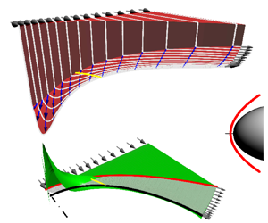
Shock waves are distinctive features in high-speed compressible flow fields. Complicated flow patterns with shock reflections and interferences, along with the separated supersonic and subsonic regions, see figure 1, usually result in extremely high aerothermal loads or non-uniform pressure distributions. The geometries of these patterns are important features for the precise analysis and have already aroused extensive research interest.

Figure 1. Typical flow patterns of high-speed flow fields: (a) shock interference between a launch vehicle and a booster, (b) Mach reflection in an inward-turning inlet: (—–, red), shock wave; (- - - - -, blue) dashed line, slipline; ( $\circ$) supersonic region; (
 $\bullet$) subsonic region.
Among these studies, the Mach reflection (Mach Reference Mach1878) is one of the typical research interests in recent years. Based on the classical shock relations and the three shock theory (von Neumann Reference von Neumann1943, Reference von Neumann1945), analytical prediction models for the height of the Mach stem have been established by Azevedo (Reference Azevedo1989), Azevedo & Liu (Reference Azevedo and Liu1993) and Li & Ben-Dor (Reference Li and Ben-Dor1997), following different assumptions for the position of the sonic throat. Mouton (Reference Mouton2006) suggested another model based on the geometrical relationship between the straight segments of shock waves and expansion waves. Gao & Wu (Reference Gao and Wu2010) further improved these models with additional details, such as transmitted expansion waves and the Mach waves generated from the slipline. In these models, a quasi-one-dimensional isentropic relation was applied in the subsonic pocket, where the mass-averaged pressure is used to balance that above the slipline. The shape of the Mach stem was also studied by a series of analytical models (Li, Ben-Dor & Han Reference Li, Ben-Dor and Han1994; Li & Ben-Dor Reference Li and Ben-Dor1997; Tan, Ren & Wu Reference Tan, Ren and Wu2005). Based on these models, geometries of the flow patterns have been studied in various conditions, such as the asymmetric Mach reflections (Tao et al. Reference Tao, Liu, Fan, Xiong, Yu and Sun2017; Lin, Bai & Wu Reference Lin, Bai and Wu2019) and the reflections on a non-flat plane (Yao, Li & Wu Reference Yao, Li and Wu2013). Bai & Wu (Reference Bai and Wu2017) further considered the shapes of the slipline and the reflected shock wave, which are disturbed by the secondary Mach waves and the expansion fan. They also studied the effect of the trailing wedge height on the Mach stem (Bai & Wu Reference Bai and Wu2021). For the internal axisymmetric flow, Shoesmith & Timofeev (Reference Shoesmith and Timofeev2021) provided a model that combined the method of characteristics with the equations for the quasi-one-dimensional flow. For a curved-shock wave reflecting on a flat plane, Zhang et al. (Reference Zhang, Xu, Shi, Zhu and You2023) provided the shock geometries and transition criteria based on the method of curved-shock characteristics (Shi et al. Reference Shi, Zhu, You and Zhu2021), where the quasi-one-dimensional assumption was also applied for calculating the height of the sonic throat.
Another typical research interest is the stand-off distance of a bow shock wave detached from a blunt body, where the downstream consists of both subsonic and supersonic regions. Due to the theoretical difficulties, various assumptions were proposed for the applicable approximations in a wide range of the free-stream Mach numbers. Moeckel (Reference Moeckel1921) simplified the shape of the shock wave as a hyperbola, for it is the simplest analytical expression satisfying the geometrical features. Then the stand-off distance was obtained by assuming the sonic line was straight. Other assumptions, e.g. rotational incompressible flow (Hida Reference Hida1953) and a constant density behind the shock (Lighthill Reference Lighthill1957), were also proposed. Empirical regressions were obtained from various experimental sources (Ambrosio & Wortman Reference Ambrosio and Wortman1962; Billig Reference Billig1967), which are still applicable as the fast prediction method to this day. Recently, Sinclair & Cui (Reference Sinclair and Cui2017) proposed another theoretical approximation for a circular cylinder, based on the modified Newtonian impact theory. Zelalem, Timofeev & Molder (Reference Zelalem, Timofeev and Molder2018) also provided analytical expressions for a two-dimensional circular cylinder and a three-dimensional sphere, based on the curved-shock theory. However, due to the absence of a purely theoretical method in the subsonic region, various assumptions are still required to describe the distributions from the shock wave to the wall.
Theoretical methods in the subsonic regions are regarded as one of the common difficulties for the above-mentioned research interests. Approximations have to be assumed, e.g. the mass-averaged properties for the Mach reflection or the predefined downstream distributions for the bow shock wave. Subsonic regions are also considered to be an important issue in other flow patterns, e.g. the type IV shock interference (Edney Reference Edney1968a,Reference Edneyb; Grasso et al. Reference Grasso, Purpura, Chanetz and Délery2003; Guan, Bai & Wu Reference Guan, Bai and Wu2020; Bai & Wu Reference Bai and Wu2022). Another difficulty might be associated with the curved streamlines, which are usually caused by the wall shapes or the three-dimensional effects. Since the downstream flow properties are varied from the immediate after-shock conditions, the complexities of the theoretical analysis are significantly aggravated. As a result, a unified fast and accurate method is still necessary for predicting the geometries of shock waves and streamlines, no matter whether in the subsonic or supersonic regions.
To the best of the authors’ knowledge, two theoretical approaches are associated with the geometries of shock waves or streamlines. The first is the geometrical shock dynamics (GSD). Based on the Chester–Chisnell–Whitham relationship (Chester Reference Chester1954, Reference Chester1960; Chisnell Reference Chisnell1955; Whitham Reference Whitham1958; Chisnell & Yousaf Reference Chisnell and Yousaf1982), Whitham (Reference Whitham1957, Reference Whitham1959) proposed this simple and quick approach on an orthogonal mesh. It was used to solve the position and shape of a propagating shock wave. Henshaw, Smyth & Schwendeman (Reference Henshaw, Smyth and Schwendeman1986) improved the corresponding numerical method. A good review of GSD was provided by Han & Yin (Reference Han and Yin2001). According to this theory, a shock–shock disturbance is formed on a shock wave moving past a sharp obstacle. The trajectory of this disturbance is also comparable to a steady shock wave. By this means, Xiang et al. (Reference Xiang, Wang, Teng, Yang and Jiang2016) studied the three-dimensional interaction of planar shock waves on two intersecting wedges. However, on a shock wave moving past a blunt obstacle, the shock–shock disturbance is not comparable to the detached shock wave in a steady flow field. Thus the subsonic downstream is difficult to predict.
Another related theory is the curved-shock theory (CST). Based on the early studies (Crocco Reference Crocco1937; Thomas Reference Thomas1949; Gerber & Bartos Reference Gerber and Bartos1960; Emanuel & Liu Reference Emanuel and Liu1988), Mölder (Reference Mölder2012, Reference Mölder2016) derived the curved-shock equations for the streamline curvature and streamwise gradient of pressure immediately after the shock, in two-dimensional planar or axisymmetric flow fields. Recently, the CST was extended to three-dimensional non-symmetric shock waves by Emanuel & Mölder (Reference Emanuel and Mölder2022). Although the derivation is complicated, these equations can be applied to the subsonic after-shock properties. Based on the curvatures solved from the curved-shock equations, coordinates of streamlines can be approximated by a Taylor series function (Mölder Reference Mölder2017; Filippi & Skews Reference Filippi and Skews2018; Surujhlal & Skews Reference Surujhlal and Skews2018). The second-order CST was proposed by Shi et al. (Reference Shi, Han, Deiterding, Zhu and You2020) and the accuracy of predictions was improved. To further improve the accuracy, Shi et al. (Reference Shi, Zhu, You and Zhu2021) developed a method of curved-shock characteristics (MOCC) for analysis and inverse design in supersonic flow fields. In their method, the downstream of the shock wave was precisely solved by a modified method of characteristics, where the boundary conditions were given by the gradients from CST. Many flow patterns have been studied with MOCC, showing significant improvements in the accuracy, efficiency and adaptability (Cheng et al. Reference Cheng, Yang, Zheng, Shi, Zhu and You2022; Shi et al. Reference Shi, You, Zheng and Zhu2023; Zhang et al. Reference Zhang, Xu, Shi, Zhu and You2023).
As of now, theoretical methods have already been widely applied in supersonic flow fields, where the characteristic lines are the key prerequisite for establishing the coordinate system (Lewis & Sirovich Reference Lewis and Sirovich1981). However, characteristic lines are no longer available in steady subsonic flow fields, due to the complex eigenvalues of the elliptical Euler equations. To provide a unified method also available in the subsonic regions, the curves orthogonal to the streamlines are selected for the curvilinear coordinate system. Along these curves, the streamline geometries, e.g. curvatures, directions and positions, could be described by differential geometry theories (Chern, Chen & Lam Reference Chern, Chen and Lam2000). Together with the conservation laws, the flow properties, e.g. speeds and pressures, could also be solved. Once the relationships of streamline geometries and flow properties are determined, the solutions of the flow fields could be figuratively regarded as that the streamlines are reshaped to fill the domains and satisfy the boundary conditions. Based on this idea, the streamline transformation method for both subsonic and supersonic regions could be provided.
The steady inviscid compressible flow fields are considered in this study. In § 2, the relationships of streamline geometries are described based on the differential geometry theories. Accordingly, the concept and principle of the streamline transformation method are proposed. In § 3, the governing equations are derived in the regions where the properties are continuously differentiable. Four types of boundary conditions along streamlines are also introduced for the governing equations. In § 4, discontinuities in supersonic flow fields, e.g. shock waves and Mach waves, are also discussed, resulting in the shock boundary conditions and the weak discontinuity corrections. In § 5, the streamline transformation method is numerically verified, by the purely subsonic and supersonic flow fields, and also by the transitions from subsonic to supersonic regions. In the test case of the two-dimensional channel flow, which is comparable to the subsonic pocket in Mach reflections, the deviations from the quasi-one-dimensional relations are calculated. In the test case of the hyperbolic-shaped bow shock wave, the stand-off distances, sonic line shapes and three-dimensional effects are also discussed. Finally, the major conclusion of this study is summarized in § 6.
2. Streamline geometries and streamline transformation methods
Geometrical properties of streamlines are first defined in § 2.1, where the relationships between adjacent streamlines are also derived via the differential geometry theories. Following these relationships, the concept and principle of the streamline transformation method are proposed and illustrated in § 2.2.
2.1. Differential geometry for streamlines
In an arbitrary flow field, the stream surface  $\varSigma$ is defined as the surface formed by a series of streamlines, see figure 2. Orthogonal curves of the streamlines could always be generated in
  $\varSigma$, by Schmidt orthogonalization. They are named the orthogonal lines hereinafter for brevity. An orthogonal curvilinear coordinate
  $(\xi,\eta )$ is defined accordingly, where the
  $\xi$- and
  $\eta$-axes are along the streamlines and orthogonal lines, respectively. In general circumstances,
  $\varSigma$ is a curved surface. It is degraded to a flat plane in a few special cases, e.g. the two-dimensional planar or axisymmetric flow fields. Without loss of generality,
  $\varSigma$ is assumed to be curved while deriving the governing equations. It can be expressed as a mapping function
 \begin{equation} \varSigma: (\xi,\eta) \rightarrow \boldsymbol{r}(\xi,\eta)=(x,y,z)^{\rm T}, \end{equation}
where  $\boldsymbol {r}$ and
  $(x,y,z)$ are the position and Cartesian coordinates of an arbitrary point
  $P$.
$P$.

Figure 2. Orthogonal curvilinear coordinates and geometries of a stream surface: ( $\square$, green) stream surface
  $\varSigma$; (
 $\square$, cyan and
  $\square$, grey) tangential and normal planes at an arbitrary point
  $P$; (—–
 $\blacktriangleright$, black) streamlines; (- - - -
 $\blacktriangleright$, black) orthogonal lines; (
 $\cdot \!\cdot \!\cdot \!\cdot \!\cdot \cdot \!\!\blacktriangleright$, black)
  $\zeta$-axis perpendicular to
  $\varSigma$; (—–
 $\blacktriangleright$, red) curvature vector
  $\kappa _c\boldsymbol {n}_c$ of streamline, as well as its components
  $\kappa _g\boldsymbol {n}_g$ and
  $\kappa _n\boldsymbol {n}$.
The derivatives of  $\boldsymbol {r}$ with respect to
  $\xi$ and
  $\eta$ are denoted as
  $\boldsymbol {r}_\xi$ and
  $\boldsymbol {r}_\eta$. According to the orthogonal condition,
  $\boldsymbol {r}_\xi \boldsymbol {{\cdot }}\boldsymbol {r}_\eta =0$ is obtained. Thus, the first fundamental form of the stream surface
  $\varSigma$ is
 \begin{equation} \mathrm{I} = A^2\,\mathrm{d}\xi^2 + B^2\,\mathrm{d}\eta^2, \end{equation}
where  $A=|\boldsymbol {r}_\xi |$ and
  $B=|\boldsymbol {r}_\eta |$ are the metric coefficients. Along an arbitrary streamline, the length of the segment between two adjacent orthogonal lines is
  $A\,\mathrm {d}\xi$, see figure 2. Thus
  $A$ is called the length of the streamline hereinafter. For a similar reason,
  $B$ is called the distance between streamlines. Based on Gauss's theorema egregium,
  $A$ and
  $B$ are satisfied by
 \begin{equation} K ={-}\frac{1}{AB} \left[ \frac{\partial}{\partial\xi}\left(\frac{1}{A}\frac{\partial B}{\partial\xi}\right) + \frac{\partial}{\partial\eta}\left(\frac{1}{B}\frac{\partial A}{\partial\eta}\right)\right], \end{equation}
where  $K$ is the Gaussian curvature of the stream surface
  $\varSigma$. In particular,
  $K\equiv 0$ is satisfied for a flat stream surface. As the red lines with arrows in figure 2, the curvature vector of a streamline is denoted as
  $\kappa _c\boldsymbol {n}_c$. It consists of two components: the geodesic curvature
  $\kappa _g$ in the tangential plane
  $\varPi$, and the normal curvature
  $\kappa _n$ along the normal vector
  $\boldsymbol {n}$. Denoting the angle between
  $\boldsymbol {n}_c$ and
  $\boldsymbol {n}$ as
  $\varphi$ gives
 \begin{equation} \kappa_g = \kappa_c \sin\varphi,\quad \kappa_n = \kappa_c \cos\varphi. \end{equation}
The geodesic curvature  $\kappa _g$ represents how the streamline is curved in the tangential plane
  $\varPi$. Based on Liouville's formula,
  $\kappa _g$ is expressed with
  $A$ and
  $B$ as
 \begin{equation} \kappa_g ={-}\frac{1}{B} \frac{\partial\ln A}{\partial\eta}. \end{equation}
In this study, only the geodesic curvatures of streamlines would be used in the governing equations, so the streamline curvature hereinafter refers to the geodesic curvature for brevity, and the subscript  $g$ is also omitted. Substituting (2.5) into (2.3) gives
 \begin{equation} \frac{\partial A\kappa }{\partial\eta} = \frac{\partial B'}{\partial\xi} + ABK \quad \mathrm{or}\quad \frac{\partial \kappa }{\partial\eta} = B'' + B\kappa^2 + BK, \end{equation}
where  $B'$ and
  $B''$ are the first- and second-order streamwise gradients of
  $B$, expressed as
 \begin{equation} B' = \frac{1}{A}\frac{\partial B}{\partial\xi}, \quad B'' = \frac{1}{A}\frac{\partial}{\partial\xi}\left(\frac{1}{A}\frac{\partial B}{\partial\xi}\right). \end{equation}
Equation (2.6) indicates the curvature  $\kappa$ is varied along an orthogonal line, for the following three reasons:
•
 $B''\neq 0$, representing the non-uniform distances along a streamline. As displayed in figure 3(a), along a straight streamline $\eta$, a local minimum of $B$ is located at the point $P$, i.e. $B'=0$ and $B''>0$. At the points $\pm A_P\,\mathrm {d}\xi$ away from both sides of $P$, the distances between streamlines, $B_1$ and $B_2$, are expressed by a Taylor series of $B_1=B_2=B_P+B''(A\,\mathrm {d}\xi )^2/2$. Since $B_1=B_2>B_P$, the adjacent streamline $\eta +\mathrm {d}\eta$ is curved, i.e. $\kappa _Q>\kappa _P=0$. Similarly, the streamline $\eta -\mathrm {d}\eta$ is curved toward the other side, i.e. $\kappa _R<\kappa _P=0$.
•
$B\kappa ^2\neq 0$, representing the effect of streamline curvatures. Assume an arc-shaped streamline $\eta$ is curved upward, along which $B$ is distributed uniformly, see figure 3(b). Thus the adjacent streamline $\eta +\mathrm {d}\eta$ at the inward side is also a concentric arc with a smaller radius or a larger curvature, i.e. $\kappa _Q>\kappa _P>0$. Similarly, the streamline $\eta -\mathrm {d}\eta$ on the other side is less curved, i.e. $0<\kappa _R<\kappa _P$.•
$BK\neq 0$, which means the curvatures are varied following the curved stream surface.


Figure 3. Streamline curvatures varied (a) by the non-uniform distribution of  $B$ and (b) alongside a curved adjacent streamline: (—–
 $\blacktriangleright$) streamlines; (- - - -
 $\blacktriangleright$) orthogonal lines.
The direction of the streamlines, denoted as  $\theta$, is defined as the angle from a specified vector to the tangential vector
  $\boldsymbol {r}_\xi$, where the specified vector is usually selected as the direction of the incoming free stream. Based on the geometrical relationship between directions and curvatures, it gives
 \begin{equation} \kappa = \frac{1}{A}\frac{\partial \theta}{\partial\xi}. \end{equation}
Substituting (2.8) into (2.6), and integrating the result from the infinite free stream to a certain  $\xi$ gives
 \begin{equation} \frac{\partial\theta}{\partial\eta} = B' + \int_{-\infty}^\xi ABK\,\mathrm{d}\xi. \end{equation}
 Three-dimensional flow fields could be modelled by a series of parallel stream surfaces  $\varSigma _k$, where the third axis
  $\zeta$ is perpendicular to each
  $\varSigma _k$, see figure 2. In this study, the dimensionless lateral distance between stream surfaces is defined by
 \begin{equation} c = \frac{C}{C_\infty} = \frac{|\boldsymbol{r}_\zeta|}{|\boldsymbol{r}_\zeta|_\infty}, \end{equation}
where  $C=|\boldsymbol {r}_\zeta |$ is the metric coefficient along
  $\zeta$-axis, and the subscript
  $\infty$ represents the value at the infinite free stream. In a two-dimensional planar or axisymmetric flow field,
  $c$ is explicitly expressed as
 \begin{equation} c =\begin{cases} 1, & (\mathrm{planar}), \\ y/y_\infty, & (\mathrm{axisymmetric}), \end{cases} \end{equation}
where  $y_\infty$ represents the
  $y$-coordinate at the incoming free stream.
2.2. Streamline transformation methods
Based on (2.6) and (2.9) in the last subsection, the streamline geometries,  $\boldsymbol {r}$,
  $\theta$ and
  $\kappa$, could be obtained by integrations along orthogonal lines, as long as
  $B$ is known in advance. Streamline geometries are also associated with the flow properties, e.g. speeds and pressures, for the following two reasons:
• the distances
$B$ are determined by the flow speed, based on the quasi-one-dimensional flow between streamlines;• the curvatures
$\kappa$ are proportional to the gradients of pressures along orthogonal lines, based on the balance of centrifugal forces.


As a result, the relationship between streamlines is summarized as the following mapping function:
 \begin{equation} \mathop{{\mathcal{T}}_{[\xi]}}\limits_{\eta\to\eta+\mathrm{d}\eta}: \underbrace{\left[\begin{array}{@{}l@{}} \textrm{geometries} \\ \textrm{flow properties} \end{array}\right]}_{{streamline}\ \eta} \rightarrow \underbrace{\left[\begin{array}{@{}l@{}} \textrm{geometries} \\ \textrm{flow properties} \end{array}\right]}_{{streamline}\ \eta+\mathrm{d}\eta}, \end{equation}
which indicates the geometries and flow properties of streamline  $\eta +\mathrm {d}\eta$ could be calculated from those of streamline
  $\eta$, along the orthogonal line
  $\xi$. The mapping function (2.12) is also named the streamline transformation and denoted as
  ${\mathcal {T}}$, for it could be figuratively regarded as the streamline
  $\eta$ is transformed into the streamline
  $\eta +\mathrm {d}\eta$.
Based on  ${\mathcal {T}}$, the solution of flow fields in the stream surface
  $\varSigma$ could also be obtained. As illustrated in figure 4(a), assuming the geometries and flow properties on the boundary streamline
  $\eta =\eta _0$ are given, properties of all streamlines
  $\eta _1,\eta _2,\ldots$ are obtained by
  ${\mathcal {T}}$ in a certain sequence. If the flow properties of the streamline
  $\eta _0$ are unspecified, e.g. the slip wall boundary condition, numerical iterations are applied by satisfying the other side boundary conditions at the streamline
  $\eta _b$. Since the flow field is solved by the geometrical transformation of streamlines, this method is named the streamline transformation method (
 $\mathrm {STM}$) hereinafter.

Figure 4. Illustration of the streamline transformation method in (a) the continuously differentiable region and (b) the region with discontinuities: (—– $\blacktriangleright$, black) streamlines; (- - - -
 $\blacktriangleright$, black) orthogonal lines; (—–, red) shock waves; (—–
 $\blacktriangleright$, blue),
  ${\mathcal {T}}$.
Continuously differentiable geometries and flow properties are the prerequisites of the streamline transformation  ${\mathcal {T}}$. However, discontinuities are very common phenomena in the supersonic flow fields, making
  ${\mathcal {T}}$ not available across them. As illustrated in figure 4(b),
  $\varSigma$ is divided into an upstream
  $\varSigma ^-$ and a downstream
  $\varSigma ^+$ by a shock wave
  $S$. Since properties are differentiable in
  $\varSigma ^\mp$ separately, the flow field could still be solved by applying
  ${\mathcal {T}}$ in
  $\varSigma ^\mp$. The boundary conditions along
  $S$ are set from the shock theories.
Equations in  $\mathrm {STM}$ consist of various aspects, where a considerable number of mathematical derivations are inevitable. Figure 5 displays a brief diagram of these equations, where the dashed rectangle highlights the core contents, including the governing equations of
  ${\mathcal {T}}$, as well as the boundary conditions. The governing equations are partially from the differential geometries of streamlines, which have already been introduced by (2.6) and (2.9) in § 2.1. They are enclosed by the physical laws of the airflow, e.g. the mass conservation and the equilibrium of the centrifugal forces, which are derived in §§ 3.1 and 3.2, respectively. A vector-formed governing equation is concisely summarized in § 3.3. The boundary conditions along streamlines are provided and classified in § 3.4, where the algorithms are also discussed. The derivations in § 3 require the streamline geometries and flow properties to be continuously differentiable. For brevity, it is named the continuously differentiable region.

Figure 5. Diagram of equations in  $\mathrm {STM}$, as well as their mathematical derivations.
For the strong discontinuities, e.g. the shock waves,  $\mathrm {STM}$ is modified by providing the boundary conditions along the shock wave, for its upstream or downstream regions. Based on the shock relations and the curved-shock theories, properties immediately before or after the shock wave, as well as their streamwise gradients, are derived in §§ 4.1.1–4.1.3. Finally, the boundary conditions along the shock wave are introduced in § 4.1.4.
The weak discontinuities, e.g. the Mach waves, are regarded as the degradation from shock waves. Thus equations in § 4.1 are still available, from which the compatibilities of Mach waves are derived. They are similar to those from the classical theory of characteristics. Accordingly, the weak discontinuity corrections are derived in § 4.2.
3. Governing equations in continuously differentiable regions
The expressions of the streamline transformation  ${\mathcal {T}}$ are derived, based on the mass conservation in § 3.1 and the balance of centrifugal forces in § 3.2. The governing equations of
  $\mathrm {STM}$ are summarized in § 3.3 and streamline boundary conditions are introduced in § 3.4. According to the governing equations, the influencing mechanisms of the streamline geometries on the flow properties are also discussed in § 3.5.
The calorically perfect gas model is applied, where the flow properties are usually described by the Mach number  $M$ and pressure
  $p$. However, the characteristic Mach number
  $\lambda$ is used in this study to simplify the governing equations. Here,
  $\lambda$ is defined as the ratio of the local speed to the critical acoustic speed. It can be calculated from
  $M$, given by
 \begin{equation} \lambda = \sqrt{\frac{(\gamma+1)M^2}{2+(\gamma-1)M^2}}, \end{equation}
where  $\gamma$ is the specific heat ratio. By defining the upper limit of
  $\lambda$ as
  $\mu$
$\mu$
 \begin{equation} \mu=\sqrt{\frac{\gamma+1}{\gamma-1}}, \end{equation}
the isentropic relations are expressed with  $\lambda$ as
 \begin{align} \frac{p}{p_0} = \left(1-\frac{\lambda^2}{\mu^2}\right)^{(\mu^2+1)/2}, \quad \frac{\rho}{\rho_0} = \left(1-\frac{\lambda^2}{\mu^2}\right)^{(\mu^2-1)/2}, \quad \frac{T}{T_0} = \frac{a^2}{a^2_0} = 1-\frac{\lambda^2}{\mu^2}, \end{align}
where  $p_0$,
  $\rho _0$,
  $T_0$ and
  $a_0$ are the stagnation pressure, density, temperature and acoustic speed, respectively. These stagnation properties remain constants along the streamlines in the isentropic flow fields.
3.1. Mass conservation and distances between streamlines
As described in § 2.2, the distance between streamlines is determined following mass conservation. In an arbitrary element along a streamline, see figure 6, mass conservation gives
 \begin{equation} (\rho u)_{in} BC \,\mathrm{d}\eta\,\mathrm{d}\zeta = (\rho u)_{out} (B+B_\xi\,\mathrm{d}\xi) (C+C_\xi\,\mathrm{d}\xi)\, \mathrm{d}\eta\,\mathrm{d}\zeta, \end{equation}
where  $\rho$ and
  $u$ are the density and speed, respectively. Based on the isentropic relations (3.3),
  $\rho u$ is expressed with
  $\lambda$ as
 \begin{equation} \rho u = \frac{\sqrt{2}\gamma}{\sqrt{\gamma+1}} \frac{p_0/a_0}{{\mathcal{H}}(\lambda)}, \end{equation}
where  ${\mathcal {H}}$ is the function of
  $\lambda$, defined by
 \begin{equation} {\mathcal{H}}(\lambda) \equiv \frac{1}{\lambda} \left(1-\frac{\lambda^2}{\mu^2}\right)^{-(\mu^2-1)/2}. \end{equation}
With the increase of  $\lambda$,
  ${\mathcal {H}}(\lambda )$ is decreased for subsonic speeds (
 $\lambda <1$) and increased for supersonic speeds (
 $\lambda >1$). A minimum value,
  ${\mathcal {H}}(1)$, is reached at the acoustic speed. Since
  $p_0$ and
  $a_0$ remain constants along the streamline, by substituting (3.5) into (3.4) and omitting higher-order infinitesimals, we obtain
 \begin{equation} \frac{1}{BC} \frac{\partial(BC)}{\partial\xi} = \frac{1}{{\mathcal{H}}(\lambda)}\frac{\mathrm{d}{\mathcal{H}}(\lambda)}{\mathrm{d}\lambda}\frac{\partial \lambda}{\partial\xi}. \end{equation}
Integrating the above equation from the infinite free stream to a certain  $\xi$, the mass conservation (3.4) is simply expressed as
 \begin{equation} \frac{BC}{{\mathcal{H}}} = \frac{(BC)_\infty}{{\mathcal{H}}_\infty}. \end{equation}
By defining
 \begin{equation} h \equiv \frac{B_\infty}{{\mathcal{H}}_\infty}\frac{{\mathcal{H}}}{c}, \end{equation}
(3.8) is further simplified as
 \begin{equation} B = h, \end{equation}
which indicates  $h$ is just the distance between streamlines. In a two-dimensional planar flow field where
  $c\equiv 1$, the distance is proportional to
  ${\mathcal {H}}(\lambda )$. The three-dimensional effect with the varying
  $c$, makes the streamlines become close to or move away from each other.

Figure 6. Element in a streamline: the flow speeds, centrifugal forces and curvatures.
Substituting (3.10) into (2.6) and (2.9), the  $\eta$-derivatives of the curvature
  $\kappa$ and direction
  $\theta$ are given by
 \begin{equation} \frac{\partial A\kappa}{\partial\eta} = A(h''+hK)\quad \mathrm{or}\quad \frac{\partial\kappa}{\partial\eta} = h'' + h\kappa^2 + hK, \end{equation}
and
 \begin{equation} \frac{\partial\theta}{\partial\eta} = h'+F, \end{equation}
respectively, where  $h'$ and
  $h''$ are the first- and second-order streamwise gradients of
  $h$, and
  $F$ represents the effects of the curved stream surface. They are expressed as
 \begin{equation} h' = \frac{1}{A}\frac{\partial h}{\partial\xi}, \quad h'' = \frac{1}{A}\frac{\partial}{\partial\xi}\left(\frac{1}{A}\frac{\partial h}{\partial\xi}\right), \quad F = \int_{-\infty}^\xi hAK \,\mathrm{d}\xi. \end{equation}
3.2. Centrifugal forces and streamline curvatures
As described in § 2.2, the centrifugal force acting on an arbitrary element of the streamline is balanced by the pressure gradient. As displayed in figure 6, the three-dimensional centrifugal force in the reverse direction of  $\boldsymbol {n}_c$ is given by
 \begin{equation} F_c ={-} (\rho ABC \,\mathrm{d}\xi\,\mathrm{d}\eta\,\mathrm{d}\zeta) \left(M^2 \frac{\gamma p}{\rho}\right) \kappa_c. \end{equation}
Considering the geometrical relationship among curvatures (2.4), the component of  $F_c$ in the tangential plane
  $\varPi$ is expressed as
 \begin{equation} F_g = F_c\sin\varphi ={-} (\rho ABC \,\mathrm{d}\xi\,\mathrm{d}\eta\,\mathrm{d}\zeta) \left(M^2 \frac{\gamma p}{\rho}\right) \kappa. \end{equation}
Since  $F_g$ is balanced by the pressure gradients along orthogonal lines, this gives
 \begin{equation} {-}(\rho ABC \,\mathrm{d}\xi\,\mathrm{d}\eta\,\mathrm{d}\zeta) \left(M^2 \frac{\gamma p}{\rho}\right) \kappa = \left(\frac{\partial p}{\partial\eta}\,\mathrm{d}\eta\right) AC \,\mathrm{d}\xi\,\mathrm{d}\zeta. \end{equation}
Replacing  $p$ in (3.16) with the isentropic relations (3.3) gives
 \begin{equation} \frac{\partial\ln \lambda}{\partial\eta} = {\mathcal{P}} + B\kappa, \end{equation}
where
 \begin{equation} {\mathcal{P}} \equiv \frac{1}{\gamma M^2}\frac{\partial\ln p_0}{\partial\eta}, \end{equation}
representing the difference of  $p_0$ between adjacent streamlines.
Replacing  $\kappa$ in (3.17) with Liouville's formula (2.5) gives
 \begin{equation} \frac{\partial\ln A\lambda}{\partial\eta} = {\mathcal{P}}. \end{equation}
In the case that  $p_0$ is uniform at the infinite free stream, i.e.
  ${\mathcal {P}}\equiv 0$, (3.19) is further simplified as
 \begin{equation} A\lambda=\mathrm{const}. \end{equation}
It indicates the length of streamlines is inversely proportional to  $\lambda$ along an orthogonal line.
By defining the equivalent curvature
 \begin{equation} k \equiv \frac{B_\infty}{{\mathcal{H}}_\infty}\frac{\kappa}{c}, \end{equation}
and the function
 \begin{equation} {\mathcal{L}}(\lambda) \equiv \int\frac{\mathrm{d}\lambda}{\lambda {\mathcal{H}}} = {}_2F_1\left(\frac{1}{2},\,-\frac{\mu^2-1}{2};\,\frac{3}{2};\,\frac{\lambda^2}{\mu^2}\right) \lambda, \end{equation}
where  ${}_2F_1(a,b;c;z)$ is the Gaussian hypergeometric function, (3.17) is also simplified as
 \begin{equation} \frac{\partial{\mathcal{L}}}{\partial\eta} = \frac{{\mathcal{P}}}{{\mathcal{H}}} + k. \end{equation}
Here,  ${\mathcal {L}}(\lambda )$ is a monotonically increasing function of
  $\lambda$ with
  ${\mathcal {L}}(0)=0$. As a result, (3.23) represents how the flow speed is affected by the streamline curvatures. Especially in the region where
  ${\mathcal {P}}\equiv 0$,
  ${\mathcal {L}}(\lambda )$ is proportional to the equivalent curvature
  $k$. Besides, since
  $k$ is varied with
  $c$, the flow speed is also changed by the three-dimensional effects.
3.3. Governing equations
Four equations have already been derived, including that for the characteristic Mach number (3.23), as well as those for the length (3.19), curvature (3.11) and direction (3.12) of the streamlines. As it turns out, four variables,  $\lambda$,
  $A$,
$A$,  $\kappa$ and
  $\theta$, are applied for the geometries and flow properties of the streamlines. Besides, the following implied variables are also included:
•
$p_0$ for calculating the derivatives ${\mathcal {P}}$, which is always equal to the given $p_{0,\infty }$ in isentropic flow fields;•
$c$, $K$ and $F$ for the three-dimensional effect, which could be calculated from the coordinates of stream surfaces.


For two-dimensional planar flow with  $c\equiv 1$,
  $K\equiv 0$ and
  $F\equiv 0$, (3.19), (3.23), (3.11) and (3.12) have already formulated enclosed equations for
  $\lambda$,
  $A$,
$A$,  $\kappa$ and
  $\theta$. In other circumstances, equations for coordinates of streamlines are also required and expressed as
 \begin{equation} \frac{\partial x}{\partial\eta} ={-}h\sin\theta, \quad \frac{\partial y}{\partial\eta} = h \cos\theta, \end{equation}
which are applied to the flat stream surfaces parallel to the  $xy$-plane. In the general three-dimensional flow fields, the principal curvatures of the stream surfaces are used to calculate the curvatures, torsions and spatial coordinates of the orthogonal lines. Besides, multiple stream surfaces should also be considered, which remains to be further studied.
As a result, the enclosed governing equations in one stream surface are summarized as the following vector form:

where  $\boldsymbol {U}$ is named the streamline variable. Once
  $\boldsymbol {U}$ is given, the streamline geometries and flow properties are obtained in the following steps:
•
$\lambda$ is solved from the second element $U_b$ according to (3.22), expressed as $\lambda ={\mathcal {L}}^{-1}(U_b)$;•
$A$ is calculated from the first element $U_a$ by $A=\lambda ^{-1}\exp (U_a)$;•
$\kappa$ is calculated from the third element $U_c$ by $\kappa =U_c/A$;•
$\theta$, $x$ and $y$ are directly the fourth–sixth elements of $\boldsymbol {U}$;•
$h$ is directly calculated by (3.9);• derivatives
$h'$ and $h''$ are obtained from the numerical finite-difference schemes.


Under general circumstances, the analytic expression is difficult to solve from (
3.25), but the numerical result is easily obtained. For brevity, the solution is expressed as
 \begin{equation} \boldsymbol{U}(\xi,\eta+\mathrm{d}\eta) = \mathop{{\mathcal{T}}_{[\xi]}}\limits_{\eta\to\eta+\mathrm{d}\eta} [\boldsymbol{U}(\xi,\eta)], \end{equation}
which is regarded as the detailed expression of the streamline transformation (2.12).
The derivation of (3.26) is not restricted by the flow speed, no matter whether it is subsonic or supersonic. As a result, the streamline transformation  ${\mathcal {T}}$ is applicable to flow fields with purely subsonic/supersonic regions and also transitions from subsonic and supersonic regions. From a mathematical perspective, the major difference might be that it is elliptic in subsonic regions and hyperbolic in supersonic regions, due to
  ${\mathcal {H}}(\lambda )$ being monotonically decreasing and increasing, respectively.
3.4. Streamline boundary conditions
As described in § 2.2, boundary conditions should be set to the streamlines  $\eta _0$ and
  $\eta _b$. The following four types are commonly applied as the streamline boundary conditions.
• Type I: the geometries and flow properties are all given. The boundary condition is expressed as
(3.27a)Here,\begin{equation} \eta = \eta_0:\; \boldsymbol{r}=\boldsymbol{r}_0(\xi), \quad \lambda = \lambda_0(\xi). \end{equation}$A$, $\theta$ and $\kappa$ are calculated from $\boldsymbol {r}$ based on the geometrical relationships and $h$, $h'$ and $h''$ are also obtained from $\lambda$, $A$ and $\boldsymbol {r}$ following their definitions. Thus $\boldsymbol {U}_0(\xi )$ is obtained.• Type II: the geometries are given by
(3.27b)while the flow properties are unspecified. Type II boundary is also known as the slip wall.\begin{equation} \eta = \eta_{w}: \; \boldsymbol{r}=\boldsymbol{r}_{w}(\xi), \end{equation}• Type III:
$\lambda$ is given by the infinite free stream
(3.27c)while the geometries are unspecified. It is also known as the far-field boundary.\begin{equation} \eta = \eta_\infty: \; \lambda = \lambda_\infty, \end{equation}• Type IV:
$\lambda$ along the streamline boundary is calculated from the specified pressure $p_p(\xi )$, given by
(3.27d)while the geometries are unspecified. It is also known as the pressure boundary.\begin{equation} \eta = \eta_p: \; \lambda = \lambda_p(\xi) = \mu\sqrt{1 - \left[\frac{p_p(\xi)}{p_0}\right]^{2/(\mu^2+1)}}, \end{equation}


In the flow field with type I boundary conditions, streamline variables are directly calculated by  ${\mathcal {T}}$ in a certain sequence, expressed as
 \begin{equation} \boldsymbol{U}(\xi,\eta) = \mathop{{\mathcal{T}}_{[\xi]}}\limits_{\eta_0\to\eta} [\boldsymbol{U}_0(\xi)] = \mathop{{\mathcal{T}}_{[\xi]}}\limits_{\eta-\mathrm{d}\eta\to\eta} \ldots \mathop{{\mathcal{T}}_{[\xi]}}\limits_{\eta_1\to\eta_2} \mathop{{\mathcal{T}}_{[\xi]}}\limits_{\eta_0\to\eta_1} [\boldsymbol{U}_0(\xi)], \end{equation}
where  $\boldsymbol {U}_0(\xi )$ is the given streamline variable at the boundary
  $\eta _0$. For the other types of boundary conditions, numerical iterations are usually required.
As an illustration, in figure 7, a slip wall boundary (type II) is set to the streamline  $\eta _0$, and the type II–IV boundaries are set to the streamline
  $\eta _b$, respectively. The representative flow fields are (a) the flow through channels, (b) the external flow of an airfoil and (c) the subsonic pocket in the Mach reflection. The streamline variable
  $\boldsymbol {U}_0^{\dagger} (\xi )$ at the boundary
  $\eta _0$ is the numeric solution satisfying the conditions of convergence
 $$\begin{gather} \lVert \boldsymbol{r}[\boldsymbol{U}_b^{\dagger}(\xi)] - \boldsymbol{r}_{{w}2}(\xi) \rVert_{\eta_b} \leq \mathrm{restol}, \end{gather}$$
 $$\begin{gather}\lVert \lambda[\boldsymbol{U}_b^{\dagger}(\xi)] - \lambda_\infty \rVert_{\eta_b} \leq \mathrm{restol}, \end{gather}$$
 $$\begin{gather}\lVert \lambda[\boldsymbol{U}_b^{\dagger}(\xi)] - \lambda_p(\xi) \rVert_{\eta_b} \leq \mathrm{restol}, \end{gather}$$
where the functions  $\boldsymbol {r}[\boldsymbol {U}]$ and
  $\lambda [\boldsymbol {U}]$ represent the spatial coordinates and the characteristic Mach number calculated from the streamline variable
  $\boldsymbol {U}$. The streamline variable
  $\boldsymbol {U}_b^{\dagger} (\xi )$ at the boundary
  $\eta _b$ is supposed to be calculated by
  ${\mathcal {T}}$ sequentially, given by
 \begin{equation} \boldsymbol{U}_b^{\dagger}(\xi) = \mathop{{\mathcal{T}}_{[\xi]}}\limits_{\eta_0\to\eta_b}[\boldsymbol{U}_0^{\dagger}(\xi)] = \mathop{{\mathcal{T}}_{[\xi]}}\limits_{\eta_{b}-\mathrm{d}\eta\to\eta_b} \ldots \mathop{{\mathcal{T}}_{[\xi]}}\limits_{\eta_1\to\eta_2} \mathop{{\mathcal{T}}_{[\xi]}}\limits_{\eta_0\to\eta_1} [\boldsymbol{U}_0^{\dagger}(\xi)]. \end{equation}
Figure 7. Boundary conditions of (a) wall/wall, (b) wall/far field and (c) wall/pressure: (—– $\blacktriangleright$, black) streamline boundaries; (- - - -
 $\blacktriangleright$, black) orthogonal lines.
However, in actual practice, since the intermediate  $\boldsymbol {U}^{(n)}(\xi,\eta _0)$ in the
  $n$th iteration is different from
  $\boldsymbol {U}_0^{\dagger} (\xi )$, their errors are accumulated and amplified quickly by the transformation sequence. Numerical divergences are always observed. To overcome the divergence problem, an inverse prediction of
  $\lambda$ is introduced. Before the transformation from the streamlines
  $\eta$ to
  $\eta +\mathrm {d}\eta$,
  $\lambda {(\xi,\eta )}$ is replaced by
 \begin{equation} \lambda^{*}{(\xi,\eta)} = (1-\omega)\lambda{(\xi,\eta)} + \omega \lambda^\circ{(\xi,\eta)}, \end{equation}
where  $\lambda ^\circ (\xi,\eta )$ is calculated with the intermediate value at the targeting streamline
  $\eta +\mathrm {d}\eta$, based on the governing equation (3.25b). It is expressed as
 \begin{equation} \lambda^\circ(\xi,\eta) = {\mathcal{L}}^{{-}1} \left\{ {\mathcal{L}}[\lambda(\xi,\eta+\mathrm{d}\eta)] - \left(\frac{{\mathcal{P}}}{{\mathcal{H}}}+\frac{\kappa}{\sigma c}\right)_{(\xi,\eta)}\mathrm{d}\eta \right\}. \end{equation}
In (3.31),  $\omega$ is the relaxation factor to improve the numerical stabilities, which is selected to be around 0.1–0.2 in this study. Once
  $\lambda ^*$ is calculated from (3.31), the corresponding streamline variable
  $\boldsymbol {U}^*$ is then applied by the streamline transformation
  ${\mathcal {T}}$.
3.5. Influencing mechanisms of streamline geometries on flow properties
The governing equations (3.25) indicate the streamline geometries and flow properties are strongly associated, as summarized in table 1. The condition  $\xi =\mathrm {const}$ or
  $\eta =\mathrm {const}$ means a certain rule holds along an orthogonal line
  $\xi$ or a streamline
  $\eta$. Here,
  ${\mathcal {P}}\equiv 0$,
  $F\equiv 0$ and
  $c\equiv 1$ represent the uniform stagnation pressures, flat stream surfaces and two-dimensional planar flow fields, respectively. The following two rules in table 1 are discussed in depth:
•
$B=h$ indicates the distance between streamlines is determined by $h$. In the two-dimensional planar flow fields where $c\equiv 1$, $B$ is proportional to ${\mathcal {H}}$. With an increase of $\lambda$, the streamlines become convergent in subsonic regions or divergent in supersonic regions, e.g. the flow field in a nozzle. In the three-dimensional flow fields, $c$ is also an important influencing factor of $B$. As the increase of $c$, streamlines are also getting close to each other, e.g. the downstream of a conical shock wave.•
$k={\mathcal {L}}_\eta$ indicates the variation of ${\mathcal {L}}$ along an orthogonal line is proportional to the equivalent curvature $k$. As a result, alongside a curved streamline, ${\mathcal {L}}$ is larger at the inward-turning side, while it is smaller at the other side. It is reflected in various situations, e.g. the external flow past an airfoil and the internal flow along a curved wall.


Table 1. Relationships between geometries and flow properties of streamlines.

Finally, the influencing mechanics of the streamline geometries on the flow properties are summarized as:
(i) the flow speeds are varied by
$k$, the equivalent curvatures, and also determined by $h$, the distances between streamlines;(ii) three-dimensional effects are regarded such that
$h$ and $k$ are changed by $c$, which is the dimensionless lateral distance between stream surfaces.


4. Discontinuities in supersonic regions
Discontinuities are very common phenomena in supersonic flow fields, categorized by strong discontinuities and weak discontinuities. Across a strong discontinuity, the flow speed and streamline direction are changed immediately, e.g. shock waves. For the strong discontinuities, a shock boundary condition for the upstream or downstream regions is derived in § 4.1. Across a weak discontinuity, properties remain unchanged, but their gradients are changed immediately, e.g. the frontier Mach wave of an expansion fan. For the weak discontinuities, a weak discontinuity correction for the streamline transformation  ${\mathcal {T}}$ is introduced in § 4.2.
4.1. Shock waves and shock boundary conditions
On each side of a shock boundary, values required for the governing equations (3.25) consist of the zero-order properties, e.g.  $\lambda$,
  $h$,
$h$,  $\theta$,
  $A$, the first-order properties, e.g.
  $\kappa$ and
  $h'$ and the second-order property
  $h''$.
Before deriving the shock boundary conditions, notations are first illustrated in figure 8. The coordinates of a shock wave  $S$ in the stream surface
  $\varSigma$ are given by
 \begin{equation} S: s\to\boldsymbol{r}(s) = \boldsymbol{r}[\xi(s),\eta(s)], \end{equation}
where  $s$ is the arc length coordinate along
  $S$. According to (4.1), the tangential vector is expressed as
 \begin{equation} \dot{\boldsymbol{r}}(s) = \frac{\mathrm{d}\boldsymbol{r}(s)}{\mathrm{d}s} = \frac{\mathrm{d}\xi(s)}{\mathrm{d}s}\boldsymbol{r}_\xi + \frac{\mathrm{d}\eta(s)}{\mathrm{d}s}\boldsymbol{r}_\eta. \end{equation}
The shock wave direction  $\chi (s)$ is defined by the angle from a pre-specified axis to
  $\dot {\boldsymbol {r}}(s)$. The shock wave curvature
  $\kappa _S$ is defined by the derivative of
  $\chi$ with respect to
  $s$, i.e.
  $\kappa _S(s)=\dot {\chi }$. Properties immediately before and after the shock wave
  $S$ are denoted by the superscripts
  $-$ and
  $+$. For instance,
  $\lambda ^\mp$,
  $p_0^\mp$ and
  $\theta ^\mp$ are the characteristic Mach numbers, stagnation pressures and streamline directions. The shock angle is defined by
  $\beta ^-=\chi -\theta ^-$. For symmetry, a downstream shock angle is also defined by
  $\beta ^+=\chi -\theta ^+$, representing the angle between the downstream streamline and the shock wave. An additional variable,
  $\varrho =\mathrm {sgn}\,\beta ^\mp$, is defined to distinguish the left-running (
 $\varrho =1$) and right-running (
 $\varrho =-1$) shock waves. The stream surface
  $\varSigma$ is selected where the normal vectors are always perpendicular to both the upstream and downstream streamlines, making
  $\varSigma$ still smooth along
  $S$ and satisfying
 \begin{equation} c^-=c^+. \end{equation}
For brevity, the superscript  $\mp$ is omitted hereinafter, except when both the upstream and downstream properties exist in the same equation.

Figure 8. Definitions of upstream and downstream properties of the (a) left-running shock wave and(b) right-running shock wave: (—– $\blacktriangleright$, black) streamlines; (—–, red) shock waves.
The properties mentioned above could always be calculated based on the classical shock relations and the CST, which are usually expressed with the upstream  $M^-$ and
  $\beta ^-$. For the streamline transformation
  ${\mathcal {T}}$ to be applied,
  $M^-$ should be replaced with
  $\lambda ^-$, which is always feasible according to (3.1). However, the resulting expressions are too complicated. For simplicity, it would be desirable to express all these properties by unified expressions on each side. By introducing two shock invariants which remain unchanged across the shock wave, expressions for the shock boundary conditions are expected to become more concise.
Under this consideration, the shock invariants are first introduced in § 4.1.1. Then the first- and second-order properties of streamlines are derived in § 4.1.2 and § 4.1.3, respectively. Finally, the shock boundary conditions are summarized in § 4.1.4.
4.1.1. Shock invariants
On an arbitrary element along the shock wave, according to the conservation laws of mass, momentum and energy,we have the following two shock invariants:
 $$\begin{gather} {\mathcal{S}} \equiv \frac{[(\mu^2+1)\sin^2\beta^\mp-1]\lambda^\mp+ \mu^2/\lambda^\mp}{2\mu^2\sin\beta^\mp}, \end{gather}$$
 $$\begin{gather}{\mathcal{D}} \equiv\pm\frac{[(\mu^2-1)\sin^2\beta^\mp+1]\lambda^\mp- \mu^2/\lambda^\mp}{2\mu^2\sin\beta^\mp}. \end{gather}$$
Mathematical derivations of (4.4) are described in Appendix A. Even though they are complicated, the physical meanings of  ${\mathcal {S}}$ and
  ${\mathcal {D}}$ are simply expressed as
 \begin{equation} {\mathcal{S}} = \varrho\frac{\lambda_n^-+\lambda_n^+}{2}, \quad {\mathcal{D}} = \varrho\frac{\lambda^-_n-\lambda^+_n}{2}, \quad {\mathcal{S}}^2-{\mathcal{D}}^2 = \lambda^-_n\lambda^+_n = 1-\frac{\tau^2}{\mu^2}, \end{equation}
where  $\lambda _n^\mp$ and
  $\tau$ are the normal and tangential components of
  $\lambda ^\mp$, respectively. Equation (4.5) indicates:
•
$|{\mathcal {S}}|$ is the algebraic average of $\lambda _n^\mp$, reflecting the flow speeds across the shock wave.•
$|{\mathcal {D}}|$ is half of the difference between $\lambda _n^\mp$, representing the strength of the shock wave. In particular, the shock wave is degraded to a Mach wave when ${\mathcal {D}}=0$.• The square root of
${\mathcal {S}}^2-{\mathcal {D}}^2$ is the geometric average of $\lambda ^\mp _n$. The relationship between $\lambda _{n}^\mp$ and $\tau$ also corresponds with the classical Prandtl expression.


With  ${\mathcal {S}}$ and
  ${\mathcal {D}}$, properties on each side of the shock wave are expressed as
 $$\begin{gather} \lambda^\mp= \sqrt{\mu^2 - (\mu^2-1){\mathcal{S}}^2+(\mu^2+1){\mathcal{D}}^2 \pm 2{\mathcal{S}D}}, \end{gather}$$
 $$\begin{gather}\lambda^\mp_n = \varrho({\mathcal{S}} \pm {\mathcal{D}}), \end{gather}$$
 $$\begin{gather}\tau = \mu \sqrt{1-{\mathcal{S}}^2+{\mathcal{D}}^2}, \end{gather}$$
 $$\begin{gather}\tan\beta^\mp= \frac{{\mathcal{S}} \pm {\mathcal{D}}}{\tau} = \frac{{\mathcal{S}}\pm{\mathcal{D}}}{\mu \sqrt{1-{\mathcal{S}}^2+{\mathcal{D}}^2}}, \end{gather}$$
the deflection angle is expressed as
 \begin{equation} \tan\delta = \frac{2{\mathcal{D}}\tau}{{\mathcal{S}}^2-{\mathcal{D}}^2+\tau^2} = \frac {2\mu{\mathcal{D}}\sqrt{1-{\mathcal{S}}^2+{\mathcal{D}}^2}} {\mu^2-(\mu^2-1)({\mathcal{S}}^2-{\mathcal{D}}^2)}, \end{equation}
and the ratio of stagnation pressures is expressed as
 \begin{equation} \ln\frac{p_0^+}{p_0^-} = \frac{\mu^2+1}{2}\ln\frac{{\mathcal{S}}+{\mathcal{D}}}{{\mathcal{S}}-{\mathcal{D}}} + \frac{\mu^2-1}{2}\ln\frac{{\mathcal{S}}-\gamma{\mathcal{D}}}{{\mathcal{S}}+\gamma{\mathcal{D}}}. \end{equation}
 The relationships of streamline geometries on both sides of the shock wave are also derived. By taking the directional derivative of  $\boldsymbol {r}$ along the shock wave we have
 \begin{equation} \frac{\mathrm{d}\boldsymbol{r}}{\mathrm{d}s} = \frac{\cos\beta^\mp}{A^\mp}\boldsymbol{r}_\xi + \frac{\sin\beta^\mp}{B^\mp}\boldsymbol{r}_\eta. \end{equation}
Comparing the above expression with (4.2) gives
 \begin{equation} \frac{A^-}{B^-}\tan\beta^-= \frac{A^+}{B^+}\tan\beta^+= \frac{\mathrm{d}\eta(s)/\mathrm{d}s}{\mathrm{d}\xi(s)/\mathrm{d}s}, \end{equation}
and
 \begin{equation} \frac{A^+}{A^-} = \frac{\cos\beta^+}{\cos\beta^-}, \quad \frac{B^+}{B^-} = \frac{\sin\beta^+}{\sin\beta^-}. \end{equation}
Substituting (A2a) into (4.9) gives
 \begin{equation} A^-\lambda^-= A^+\lambda^+, \end{equation}
which indicates that the length of the streamlines,  $A^\mp$, is inversely proportional to
  $\lambda ^\mp$. By coincidence, a similar relation is also concluded from (3.20), for isentropic flow fields with uniformly distributed stagnation pressures.
The decrease of the distance between streamlines across the shock wave is then illustrated in figure 9. Substituting (A3) into (4.9) to eliminate  $\sin \beta ^\mp$ gives
 \begin{equation} \frac{B^-}{{\mathcal{H}}^-{/}p_0^-} = \frac{B^+}{{\mathcal{H}}^+{/}p_0^+}. \end{equation}
According to (3.8) on each side of the shock wave  $SS'$, we have
 \begin{equation} \frac{B_Pc_P}{{\mathcal{H}}_P} = \frac{B^-c^-}{{\mathcal{H}}^-}, \quad \frac{B_Qc_Q}{{\mathcal{H}}_Q} = \frac{B^+c^+}{{\mathcal{H}}^+}. \end{equation}
Since  $c^-=c^+$ from (4.3), the last two equations give
 \begin{equation} \frac{B_Qc_Q}{{\mathcal{H}}_Q/p_{0,Q}} = \frac{B_Pc_P}{{\mathcal{H}}_P/p_{0,P}}, \end{equation}
which indicates that the distance  $B$ between streamlines is always proportional to
  ${\mathcal {H}}/(p_0c)$, no matter how many shock waves have been crossed. Compared with (3.8) from mass conservation, only
  $p_0$ is added in (4.13). It is obvious that the governing equations (3.25) in § 3 still hold, by just replacing the definitions of
  $h$ and
  $k$ with
 \begin{equation} h \equiv \frac{B_\infty}{{\mathcal{H}}_\infty}\frac{{\mathcal{H}}}{\sigma c}, \quad k \equiv \frac{B_\infty}{{\mathcal{H}}_\infty}\frac{\kappa}{\sigma c}, \end{equation}
where  $\sigma =p_0/p_{0,\infty }$.

Figure 9. Elements of the shock wave intersecting with streamlines: (—–, red) shock waves; (—– $\blacktriangleright$, black) streamlines; (- - - -
 $\blacktriangleright$, black) orthogonal lines.
4.1.2. First-order properties of streamlines
Following the derivation of the first-order curved-shock equations (Mölder Reference Mölder2012, Reference Mölder2016), by taking the directional derivatives of  ${\mathcal {L}}$ and
  $\theta$ to
  $s$, where the
  $\eta$-derivatives in the results are replaced with the governing equations (3.25b) and (3.25d), equations about
  $\kappa$ and
  $h'$ on each side of the shock wave are finally obtained as
 \begin{equation} \left[\begin{array}{@{}cc@{}} \cos\beta & \sin\beta \\ \sin\beta & \varpi\cos\beta \end{array}\right] \left[\begin{array}{@{}c@{}} \kappa \\ h'/h \end{array}\right] =\left[\begin{array}{@{}c@{}} b_\kappa \\ b_h \end{array}\right], \end{equation}
where  $\varpi$ is a variable only concerned with
  $\lambda$, expressed as
 \begin{equation} \varpi = \frac{1-\lambda^2/\mu^2}{\lambda^2-1} = \frac{1}{M^2-1}. \end{equation}
Details of the derivation and verification of (4.15) are introduced in Appendix B. Elements on the right-hand side of (4.15),  $b_\kappa$ and
  $b_h$, are expressed with
  ${\mathcal {S}}$ and
  ${\mathcal {D}}$ as
 $$\begin{gather} b_\kappa = E_\theta \dot{{\mathcal{S}}} + F_\theta \dot{{\mathcal{D}}} + \dot{\varTheta} - F\sin\beta/h, \end{gather}$$
 $$\begin{gather}b_h = E_h \dot{{\mathcal{S}}} + F_h \dot{{\mathcal{D}}} - \dot{{\mathcal{Q}}}/\gamma M^2 - {\mathcal{R}}\varpi\cos\beta, \end{gather}$$
where
 \begin{align} \dot{{\mathcal{S}}} = \frac{\mathrm{d}{\mathcal{S}}}{\mathrm{d}s}, \quad \dot{{\mathcal{D}}} = \frac{\mathrm{d}{\mathcal{D}}}{\mathrm{d}s}, \quad \dot{\varTheta} = \frac{\mathrm{d}\theta^-}{\mathrm{d}s}, \quad \dot{{\mathcal{Q}}} = \frac{\mathrm{d}\ln p_0^-}{\mathrm{d}s}, \quad {\mathcal{R}} = (\ln c)' = \frac{1}{A}\frac{\partial\ln c}{\partial\xi}. \end{align}
Here,  $E$ and
  $F$ with the subscripts in (4.17) are partial derivatives with respect to
  ${\mathcal {S}}$ and
  ${\mathcal {D}}$, defined by
 \begin{equation} E_q = \frac{\partial q}{\partial{\mathcal{S}}}, \quad F_q = \frac{\partial q}{\partial{\mathcal{D}}}, \quad (q=\lambda,\beta,p,\theta,h). \end{equation}
They are expressed as (B15) and (B18) in the explicit forms. Items in (4.17) are various sources making the streamlines curved, which are roughly categorized as follows:
• Items containing
$\dot {{\mathcal {S}}}$ and $\dot {{\mathcal {D}}}$. Based on (B22), $\dot {{\mathcal {S}}}$ and $\dot {{\mathcal {D}}}$ are calculated by
(4.20)As a result, the shock wave curvatures,\begin{align} \left[\begin{array}{@{}c@{}} \dot{{\mathcal{S}}} \\ \dot{{\mathcal{D}}} \end{array}\right]= \frac{1}{(E_\theta+E_\beta) F_\lambda - E_\lambda(F_\theta+F_\beta)} \left[\begin{array}{@{}cc@{}} F_\lambda & -F_\theta-F_\beta \\ -E_\lambda & E_\theta+E_\beta \end{array}\right] \left[\begin{array}{@{}c@{}} \kappa_S-\dot{\varTheta} \\ \dot{\lambda} \end{array}\right]. \end{align}$\kappa _S$, and the derivatives of the flow speeds, $\dot {\lambda }$, could both make the streamlines curved.•
$\dot \varTheta$ and $\dot {{\mathcal {Q}}}$, representing the effects of the non-uniform upstream flow directions and stagnation pressures, respectively.• Items containing
${\mathcal {R}}$ and $F$, representing the three-dimensional effects. For a flat stream surface, $F\equiv 0$. Furthermore, for the planar and axisymmetric flow fields we have
(4.21)\begin{equation} {\mathcal{R}} =\begin{cases} 0, & (\textrm{planar}), \\ \sin\theta/y, & (\textrm{axisymmetric}). \end{cases} \end{equation}


The determinant of (4.15) is expressed as
 \begin{equation} \varDelta = \varpi\cos^2\beta-\sin^2\beta. \end{equation}
If the shock wave is not degraded to a Mach wave,  $\varDelta \neq 0$ is obtained, which means a unique solution exists. For a given shock wave, obtaining
  $\kappa _S$ from its shape, assigning
  $\dot {\lambda }^-$,
  $\dot \varTheta$ and
  $\dot {{\mathcal {Q}}}$ with the upstream conditions, and calculating
  $\dot {{\mathcal {S}}}$ and
  $\dot {{\mathcal {D}}}$ by (4.20), the first-order properties,
  $\kappa$ and
  $h'$, are finally solved from (4.15), expressed as
 \begin{equation} \left[\begin{array}{@{}c@{}} \kappa \\ h'/h \end{array}\right] =\frac{1}{\varDelta} \left[\begin{array}{@{}cc@{}} \varpi\cos\beta & -\sin\beta \\ -\sin\beta & \cos\beta \end{array}\right] \left[\begin{array}{@{}c@{}} b_\kappa \\ b_h \end{array}\right]. \end{equation}
4.1.3. Second-order properties of streamlines
Following the idea of the second-order CST (Shi et al. Reference Shi, Han, Deiterding, Zhu and You2020), equations about the second-order properties of streamlines,  $\kappa '$ and
  $h''$, could also be obtained by taking the directional derivatives of (4.15) and replacing the
  $\eta$-derivatives with (3.25). The mathematical derivations are a little tedious, see Appendix C. Only the major results are outlined here.
On each side of the shock wave,  $\kappa '$ and
  $h''$ satisfy the following equations:
 \begin{equation} \left[\begin{array}{@{}cc@{}} \cos^2\beta+\varpi^{{-}1}\sin^2\beta & 2\sin\beta\cos\beta \\ 2\sin\beta\cos\beta & \varpi\cos^2\beta+\sin^2\beta \end{array}\right] \left[\begin{array}{@{}c@{}} \kappa' \\ h''/h \end{array}\right]= \left[\begin{array}{@{}c@{}} d_\kappa \\ d_h \end{array}\right], \end{equation}
where  $d_\kappa$ and
  $d_h$ on the right-hand side are expanded as (C16). Since the second-order derivatives of the shock invariants,
  $\ddot {{\mathcal {S}}}$ and
  $\ddot {{\mathcal {D}}}$, are required by (C16), they are solved from (C21) according to the
  $\dot {\kappa _S}$ and
  $\ddot {\lambda }$ of a given shock wave.
Finally,  $\kappa '$ and
  $h''$ are solved from (4.24) and expressed as
 \begin{equation} \left[\begin{array}{@{}c@{}} \kappa' \\ h''/h \end{array}\right]= \frac{\varpi}{\varDelta^2} \left[\begin{array}{@{}cc@{}} \varpi\cos^2\beta+\sin^2\beta & -2\sin\beta\cos\beta \\ -2\sin\beta\cos\beta & \cos^2\beta+\varpi^{{-}1}\sin^2\beta \end{array}\right] \left[\begin{array}{@{}c@{}} d_\kappa \\ d_h \end{array}\right], \end{equation}
where  $\varDelta$ is the same determinant as that in the first-order equation, see (4.22).
4.1.4. Shock boundary conditions
Following the equations in §§ 4.1.1–4.1.3, the boundary conditions for each side of the shock wave are finally expressed as
 \begin{equation} \begin{array}{@{}c@{}} \xi=\xi(s) \\ \eta=\eta(s) \end{array}:\; \left\{\begin{array}{@{}l@{}} \boldsymbol{r}=\boldsymbol{r}(s), \quad \theta = \theta(s), \quad \kappa = \kappa(s), \quad A = A(s), \\ \lambda = \lambda(s), \quad h = h(s), \quad h' = h'(s), \quad h'' = h''(s), \end{array}\right. \end{equation}
where the zero-order properties,  $\theta (s)$,
  $A(s)$,
  $\lambda (s)$ and
  $h(s)$, the first-order properties,
  $h'(s)$ and
  $\kappa (s)$, as well as the second-order property,
  $h''(s)$, are all obtained. At the same time, the stagnation pressures
  $p_0$ along the streamlines are also set to
  $p_0^+$ or
  $p_0^-$ from (4.6f). Once the shock boundary condition is set, the flow fields at either side are both calculated directly by the streamline transformation
  ${\mathcal {T}}$. No iterations are required.
In actual practice, for the curved-shock wave with a given analytic expression, the curvature  $\kappa _S$ and its derivative
  $\dot {\kappa }_S$ are mathematically obtained by differentiations. If the shock wave is expressed with discretized nodes,
  $\kappa _S$ and
  $\dot {\kappa }_S$ should be calculated from a cubic spline interpolation with the not-a-knot boundary condition, to suspend the numerical oscillations.
4.2. Mach waves and weak discontinuity corrections
Mach waves are another type of common phenomenon in supersonic flow fields, where the high-order properties, e.g.  $\kappa$,
  $h'$,
$h'$,  $h''$, are not necessarily continuous. In this study, the Mach waves with discontinuous high-order properties are named discontinuous Mach waves for brevity. The streamline transformation
  ${\mathcal {T}}$ is no longer valid across them, for the properties are non-differentiable. Other Mach waves with continuous high-order properties are named ordinary Mach waves. In the region filled with ordinary Mach waves,
  ${\mathcal {T}}$ is still available. For instance, the analytic solution in the expansion fan of the Prandtl–Meyer flow field still satisfies the governing equations (3.25).
Two typical circumstances with discontinuous Mach waves are illustrated in figure 10. If the wall curvatures are different at the two sides of the point  $O$, while the directions are the same, see figure 10(a), only one discontinuous Mach wave
  $E$ is generated. If the wall directions are directly changed at the corner
  $O$, see figure 10(b), two discontinuous Mach waves,
  $E_s$ and
  $E_e$, are generated, where a series of ordinary Mach waves are filled between them. Based on the assumption that only a limited number of discontinuous Mach waves exist in the flow field, a weak discontinuity correction of
  ${\mathcal {T}}$ is required only where a discontinuous Mach wave is intersected.

Figure 10. Discontinuous Mach waves from (a) the connection with different curvatures and (b) the corner with different directions: (—–, blue) walls; (—–, orange) discontinuous Mach waves; (—–, green) ordinary Mach waves.
To provide the expressions for the weak discontinuity correction, compatibilities along an arbitrary Mach wave are first derived in § 4.2.1. Then the correction of  ${\mathcal {T}}$ is introduced in § 4.2.2.
4.2.1. Compatibilities
Since the conservation laws of mass, momentum and energy still hold for an arbitrary element along the Mach wave, proofs are obvious that the expressions for shock waves in § 4.1 are also suitable for Mach waves, by just simply assigning  ${\mathcal {D}}=0$.
Based on (4.6a)–(4.6c), the characteristic Mach number  $\lambda$, as well as its components
  $\lambda _n$ and
  $\tau$, are expressed with
  ${\mathcal {S}}$ as
 \begin{equation} \lambda = \sqrt{\mu^2-(\mu^2-1){\mathcal{S}}^2}, \quad \lambda_n = \varrho{\mathcal{S}}, \quad \tau = \mu\sqrt{1-{\mathcal{S}}^2}. \end{equation}
The Mach angle  $\beta$ is obtained from (4.6d), satisfying
 \begin{equation} \tan\beta = \frac{{\mathcal{S}}}{\tau} = \varrho\sqrt{\varpi}, \quad \sin\beta = \varrho\sqrt{\frac{\varpi}{\varpi+1}}, \quad \cos\beta = \sqrt{\frac{1}{\varpi+1}}. \end{equation}
 By assigning  ${\mathcal {D}}=0$, equations about the first-order properties are also degraded from (4.15). Before the degrading,
  $\dot {{\mathcal {S}}}$ is first calculated from (4.27), given by
 \begin{equation} \dot{{\mathcal{S}}} ={-}\frac{\lambda\dot{\lambda}}{(\mu^2-1){\mathcal{S}}}. \end{equation}
Here,  $E_q^\mp$ and
  $F_q^\mp$ are calculated from (B15) and (B18), given by
 \begin{equation}
\left.\begin{array}{@{}c@{}}
E_\lambda^\mp={-}(\mu^2-1)\dfrac{{\mathcal{S}}}{\lambda},
\quad E_\beta^\mp= \dfrac{\mu^2}{\lambda^2\tau}, \quad
E_p^\mp= 0, \quad E_\theta^\mp= 0, \\
E_h^\mp={-}(\mu^2-1)\dfrac{{\mathcal{S}}}{\lambda^2},\quad
F_\lambda^\mp= \pm\dfrac{{\mathcal{S}}}{\lambda}, \quad
F_\beta^\mp= \pm \dfrac{\tau}{\lambda^2},\\ F_p^\mp= 0,
\quad F_\theta^-=0,\quad F_\theta^+=
\dfrac{2\tau}{\lambda^2},\quad F^\mp_h
={\pm}\dfrac{{\mathcal{S}}}{\lambda^2}. \end{array}\right\}
\end{equation}
\begin{equation}
\left.\begin{array}{@{}c@{}}
E_\lambda^\mp={-}(\mu^2-1)\dfrac{{\mathcal{S}}}{\lambda},
\quad E_\beta^\mp= \dfrac{\mu^2}{\lambda^2\tau}, \quad
E_p^\mp= 0, \quad E_\theta^\mp= 0, \\
E_h^\mp={-}(\mu^2-1)\dfrac{{\mathcal{S}}}{\lambda^2},\quad
F_\lambda^\mp= \pm\dfrac{{\mathcal{S}}}{\lambda}, \quad
F_\beta^\mp= \pm \dfrac{\tau}{\lambda^2},\\ F_p^\mp= 0,
\quad F_\theta^-=0,\quad F_\theta^+=
\dfrac{2\tau}{\lambda^2},\quad F^\mp_h
={\pm}\dfrac{{\mathcal{S}}}{\lambda^2}. \end{array}\right\}
\end{equation}Substituting (4.28)–(4.30) into (4.15) gives
 \begin{equation} \left[\begin{array}{@{}cc@{}} \cos\beta & \sin\beta \\ \sin\beta & \varpi\cos\beta \end{array}\right] \left[\begin{array}{@{}c@{}} \kappa \\ h'/h \end{array}\right]= \left[\begin{array}{@{}c@{}} \dot{\theta} - F\sin\beta/h \\ \dot{\lambda}/\lambda - \dot{{\mathcal{Q}}}/\gamma M^2 - {\mathcal{R}}\varpi\cos\beta \end{array}\right], \end{equation}
where the determinant  $\varDelta =\varpi \cos ^2\beta -\sin ^2\beta =0$ and no unique solution could be obtained. This means the first-order properties of streamlines are not determined by the shape of the Mach wave.
Equation (4.31) is physically meaningful only if the two elements are linearly dependent, which gives
 \begin{equation} \kappa + \varrho\sqrt{\varpi}\left(\frac{h'}{h}+{\mathcal{R}}\right) = \frac{1}{\sin\beta} \left(\frac{\dot{\lambda}}{\lambda} - \frac{\dot{{\mathcal{Q}}}}{\gamma M^2}\right) = \dot{\theta}\sec\beta + \left({\mathcal{R}}-\frac{F}{h}\right) \tan\beta. \end{equation}
Substituting (B6) into the left-hand side of (4.32), it is simplified to
 \begin{equation} \varepsilon \equiv \underbrace{(\theta+\varrho\nu)'}_{\varepsilon_0} = \underbrace{\frac{1}{\sin\beta} \left(\frac{\dot{\lambda}}{\lambda} - \frac{\dot{{\mathcal{Q}}}}{\gamma M^2}\right)}_{\varepsilon_1} = \underbrace{\dot{\theta}\sec\beta + \left({\mathcal{R}}-\frac{F}{h}\right)\tan\beta}_{\varepsilon_2}, \end{equation}
where  $\nu$ is just the classical Prandtl–Meyer angle, satisfying
 \begin{equation} \nu(\lambda) \equiv \int \varpi^{{-}1/2}\,\mathrm{d}\ln\lambda = \sqrt{\frac{\gamma+1}{\gamma-1}}\arctan\sqrt{\frac{\gamma-1}{\gamma+1}(M^2-1)} - \arctan\sqrt{M^2-1}. \end{equation}
It is also easy to prove that (4.33) corresponds to the compatibility conditions in the classical theory of characteristics.
4.2.2. Weak discontinuity corrections
As displayed in figure 11, from an arbitrary  $P$ on a streamline, two Mach waves with the angles
  $\beta _P=\pm \arctan \sqrt {\varpi _P}$ are generated. A domain of dependence (DoD) and a range of influence (RoI) are formed between them. The streamline transformation
  ${\mathcal {T}}$ from
  $N$ to
  $P$ is located in neither DoD nor RoI. According to the theory of characteristics, properties at
  $P$ should be independent of those at
  $N$. However, if no discontinuous Mach wave is intersected with
  $\overline {NP}$, see figure 11(a), the streamline variable
  $\boldsymbol {U}_P$ could still be calculated by
 \begin{equation} \boldsymbol{U}_P = \mathop{{\mathcal{T}}_{[\xi]}}\limits_{\eta\to\eta+\mathrm{d}\eta}(\boldsymbol{U}_N). \end{equation}
Figure 11. Streamline transformation outside the DoD and RoI, where a discontinuous Mach wave is (a) not intersected and (b) intersected: (—–, orange) discontinuous Mach waves; (—–, green) ordinary Mach waves; ( $\square$, yellow) DoD and RoI; (—–
 $\blacktriangleright$, black) streamlines; (- - - -
 $\blacktriangleright$, black) orthogonal lines; (—–
 $\blacktriangleright$, blue)
  ${\mathcal {T}}$ and
  ${\mathcal {T}}^{C}$.
Assuming a left-running discontinuous Mach wave is intersected with  $\overline {NP}$ at
  $S$, see figure 11(b), the governing equations (3.25b–d) are no longer valid, as the first- and second-order properties are not available. Based on the compatibility conditions (4.33), they are corrected with
 $$\begin{gather} (\theta+\varrho\nu)' = \frac{1}{\sin\beta} \left(\frac{\dot{\lambda}}{\lambda} - \frac{\dot{{\mathcal{Q}}}}{\gamma M^2}\right), \end{gather}$$
 $$\begin{gather}(\theta+\varrho\nu)' = \dot{\theta}\sec\beta + \left({\mathcal{R}}-\frac{F}{h}\right)\tan\beta, \end{gather}$$
 $$\begin{gather}\theta' = \kappa. \end{gather}$$
The derivatives along the left-running Mach wave  $E$, e.g.
  $\dot {\lambda }$ and
  $\dot {\theta }$, are expressed as the finite-difference schemes between
  $Q$ and
  $P$, where the values at
  $Q$ are interpolated from the nodes
  $R$ and
  $N$. With a Newton–Raphson algorithm, the streamline variable at
  $P$ is numerically solved from the corrected equations (4.36). The result is expressed in the following mapping form:
 \begin{equation} \boldsymbol{U}(\xi,\eta+\mathrm{d}\eta) = \mathop{{\mathcal{T}}^{C}_{[\xi]}}\limits_{\eta\to\eta+\mathrm{d}\eta} [ \boldsymbol{U}(\xi,\eta), \boldsymbol{U}(\xi-\mathrm{d}\xi,\eta+\mathrm{d}\eta)], \end{equation}
where  ${\mathcal {T}}^{C}$ is named the weak discontinuity correction. Compared with the original transformation
  ${\mathcal {T}}$, the streamline variable
  $\boldsymbol {U}(\xi -\mathrm {d}\xi,\eta +\mathrm {d}\eta )$ at the upstream of the targeting node must also be available for
  ${\mathcal {T}}^{C}$. This is always feasible by applying the streamline transformation in a reasonable sequence.
In actual practice,  ${\mathcal {T}}$ is applied as the default transformation operator. Only when
  ${\mathcal {T}}$ is found to be intersected with a discontinuous Mach wave is it replaced with
  ${\mathcal {T}}^{C}$ and the streamline variable at its targeting node is recalculated. In the region which is confirmed to be continuously differentiable, the corrected
  ${\mathcal {T}}^{C}$ is not applied, to reduce the computational loads and improve the smoothness of the solution.
5. Verifications and applications
The streamline transformation method ( $\mathrm {STM}$) is numerically verified by the following three test cases in the two-dimensional planar and axisymmetric flow fields:
• the subsonic flow through two-dimensional channels (§ 5.1), to show how the properties are affected by the wall curvatures;
• the supersonic downstream of an attached shock wave (§ 5.2), to verify the performance for the inverse design;
• the flow fields with detached bow shock waves (§ 5.3), to demonstrate the applicability in a wide range from subsonic to supersonic speed.
As a comparison, results from computational fluid dynamics (CFD) with the same flow conditions are also provided. In CFD algorithms, a calorically perfect gas model is assumed. A density-based Euler solver is applied since the viscosity is neglected. A second-order implicit scheme is used for the time marching, where the Courant–Friedrichs–Lewy number is between 0.1 and 0.5. The inviscid flux is solved using a second-order Van Leer flux differencing scheme. The min–mod limiter is added to the spatial discretization for the suppression of numerical oscillations. Especially for the subsonic flow, a low Mach preconditioned method (Turkel Reference Turkel1987) is also applied. The grid in the computational domain is determined after the grid-independence verification, where the resolution is also sufficient to acquire clear shock waves and smooth Mach number contours. The solution is converged with two criteria: (a) each residual is reduced by at least three orders of magnitude, and (b) fluctuations of the flow properties at specified positions vanish.
5.1. Subsonic flow fields through channels
As illustrated in figure 12, a uniform incoming free stream with  $M_\infty =0.5$ (
 $\lambda _\infty \approx 0.5345$) is flowing through a two-dimensional channel with the width
  $W$. On each side of the channel, a bump with the height
  $H_{j}$ and the length
  $L_{j}$ is located at
  $x=0$ and
  $x=X_b$, where the subscripts
  $j=0,b$ represent the lower and upper walls, respectively. The shape functions of the bumps are expressed as
 \begin{equation} \left.\begin{array}{@{}c@{}} y_0 = H_0 \cos^2\dfrac{{\rm \pi} x}{L_0}, \quad x\in\left[-\dfrac{L_0}{2}, \dfrac{L_0}{2}\right], \\ y_b = W - H_b\cos^2\dfrac{{\rm \pi}(x-X_b)}{L_b}, \quad x\in\left[X_b-\dfrac{L_b}{2}, X_b+\dfrac{L_b}{2}\right]. \end{array}\right\} \end{equation}
The lower bump is started from the point  $Q$ and reaches its peak at the point
  $P$. To eliminate the disturbance from the two endpoints of the streamlines, straight wall segments are connected to both sides of the bumps. The inlet and outlet boundaries are simply set at
  $x_{in}=-1.5L_0$ and
  $x_{out}=1.5L_0$, which satisfies the boundary-independent conditions and also provides a wider flow field for the comparison with CFD.

Figure 12. Schematic diagram and dimensions of a two-dimensional channel.
In this study, three groups of wall shape parameters are considered, see table 2. A symmetric subsonic convergent-divergent flow field is formed with shape 1. With shape 2, the heights of the bumps,  $H_0$ and
  $H_b$, are increased to reach the sonic condition at
  $P$. An unsymmetric flow field is calculated with shape 3, where the upper bump is moved downstream to the position
  $X_b=1.0$ and the flow speed at
  $P$ is also approaching the sonic condition.
Table 2. Geometrical parameters of the wall shapes.

5.1.1. Results of shape 1
In the calculation with  $\mathrm {STM}$, the boundary streamline
  $\eta _0$ is located along the lower wall, with 91 nodes distributed uniformly. Starting from streamline
  $\eta _0$, 50 more streamlines are located towards the upper wall, following a bi-geometric distribution with an increasing ratio of 1.05. Following the algorithm described in § 3.4, the streamline transformation
  ${\mathcal {T}}$ with the inverse prediction (3.31) is applied, where
  ${\mathcal {T}}$ is discretized with an implicit scheme for the marching along orthogonal lines and a central difference scheme for calculating
  $\boldsymbol {F}(\boldsymbol {U})$. After the numerical iterations are converged, the contours of Mach numbers are obtained, see the black solid lines in figure 13(a). The streamline geometries are obtained accordingly, see figure 13(b), where the densities of the curves are reduced for clarity.

Figure 13. Results of shape 1: (a) contour of Mach number and (b) streamline geometries: (—–, black),  $\mathrm {STM}$; (- - - - -, black) CFD.
As a comparison, the flow field is also simulated by CFD with the same flow conditions. An inflow boundary condition is set to the inlet with the free-stream velocities. An outflow boundary is set to the subsonic outlet with the back pressure. Slip boundary conditions are set to the lower and upper walls. Based on the boundary-independent test, the inlet and outlet are located at  $x_{in}=-4L_0$ and
  $x_{out}=4L_0$, respectively. As a result, a structured grid with 18 000 cells is generated in the computational domain. The numerical algorithms of the CFD solver have already been introduced at the beginning of this section. The resulting contours of Mach numbers are also displayed in figure 13(a), see the black dashed lines.
Figure 13(a) indicates that good agreements are achieved in the region between two bumps. However, the contours of  $M=0.5$ are mismatched in the straight segments. For a quantitative analysis of the numerical errors, figure 13(b) displays three typical streamlines along the centre line, as well as the lower and upper walls. They are denoted as
  $\eta _{CL}$,
  $\eta _0$ and
  $\eta _b$, respectively. Starting from the points
  $P$,
$P$,  $Q$ and
  $(-L_0,0)$, three orthogonal lines,
  $\xi _P$,
  $\xi _Q$ and
  $\xi _I$, are also selected. The Mach numbers along these streamlines and orthogonal lines are displayed in figure 14(a,b), which indicates the results from
  $\mathrm {STM}$ are extremely similar to those from CFD. The numerical errors of
  $\mathrm {STM}$, defined by
 \begin{equation} \mathrm{error} = \frac{M_{STM}-M_{CFD}}{M_{CFD}} \times 100\,\%, \end{equation}
are displayed in figure 14(c,d). The results indicate the maximum errors are within  $\pm 1\,\%$. No evident difference between
  $\mathrm{STM}$ and CFD is observed in the straight segments, where the Mach numbers are both approximately
  $M=0.5$. Thus the mismatched contours in figure 13(a) are associated with the uniform flow field. By definition, the differential equation of a general contour line is written as
 \begin{equation} (\boldsymbol{\nabla} M) \boldsymbol{{\cdot}} (\mathrm{d}\,x,\mathrm{d} y) =0. \end{equation}
Here,  $\boldsymbol {\nabla } M\approx \boldsymbol {0}$ makes the direction
  $(\mathrm{d}\,x,\mathrm {d} y)$ undetermined and extremely sensitive. In
  $\mathrm {STM}$, the numerical errors are accumulated along the orthogonal lines from the lower wall to the upper wall, which makes the contours in these regions asymmetric and different from the CFD results. Even though the contours are not fully matched, the distributions of Mach numbers are still regarded as similar between
  $\mathrm {STM}$ and CFD.

Figure 14. Mach numbers along (a) streamlines and (b) orthogonal lines, as well as their (c,d) numerical errors, STM results: (—–, red)  $\eta _0$; (—–, green)
  $\eta _{CL}$; (—–, blue)
  $\eta _b$; (- - - - -, red)
  $\xi _P$; (- - - - -, green)
  $\xi _Q$; (- - - - -, blue)
  $\xi _I$; CFD results: (
 $\bullet$, red)
  $\eta _0$; (
 $\bullet$, green)
  $\eta _{CL}$; (
 $\bullet$, blue)
  $\eta _b$; (
 $\circ$, red)
  $\xi _P$; (
 $\circ$, green)
  $\xi _Q$; (
 $\circ$, blue)
  $\xi _I$.
The streamline directions  $\theta$ are also compared in figure 15, which indicates the maximum errors within
  $0.06^\circ$. Moreover, the shapes of streamlines from
  $\mathrm {STM}$ also fully coincide with those from CFD, as already displayed in figure 13(b), see the black solid (
 $\mathrm {STM}$) and dashed (CFD) lines.

Figure 15. Streamline directions along orthogonal lines, (a) values, (b) numerical errors STM results: (—–, red)  $\xi _P$; (—–, green)
  $\xi _Q$; (—–, blue)
  $\xi _I$; CFD results: (
 $\circ$, red)
  $\xi _P$; (
 $\circ$, green)
  $\xi _Q$; (
 $\circ$, blue)
  $\xi _I$.
5.1.2. Convergencies and stabilities
The  $\mathrm {STM}$ algorithm is also a grid-based algorithm, where the results are affected by the grid convergence. Figure 16(a,b) displays the Mach numbers varying with the number of streamlines,
  $J$, where
  $M_Q$ and
  $M_P$ are the values at the points
  $Q$ and
  $P$, representing the minimum and maximum in the flow field. As
  $J$ is increased from 21 to 201,
  $M_Q$ and
  $M_P$ are gradually levelling off and finally remain unchanged. Since high-order properties are computed in the streamline transformation, the maximum errors are still within 0.2 % and 0.53 %, respectively.

Figure 16. The  $\mathrm {STM}$ results, (a)
  $M_Q$, (b)
  $M_P$, (c) iteration steps and (d) CPU time, varying with the numbers of streamlines,
  $J$.
$J$.
The hollow points in figure 16 represent  $J=51$, which is applied in the current case. If
  $J$ is further increased, the numerical errors are expected to be reduced by only 0.05 % and 0.14 %. However, the iteration steps and CPU time are increased significantly, see figure 16(c,d). As a result,
  $J=51$ is regarded to be acceptable for both accuracy and efficiency. The computational resources consumed by
  $\mathrm {STM}$ are also compared with CFD, see table 3. The results show the node count is reduced by approximately 75 % and the flow field is solved within only 4 seconds.
Table 3. Computational loads for the subsonic flow field in the symmetric channel (shape 1).

Numerical divergences are always observed if  $J<20$. The intermediate orthogonal lines are crossed and
  $\lambda$ is approaching its upper limit
  $\mu$, until the solver is crushed. This could be explained by the governing equation (3.25b). Applying
  $c\equiv 1$,
  $\sigma \equiv 1$ and
  ${\mathcal {P}}\equiv 0$ for the two-dimensional planar flow field with a uniform stagnation pressure gives the relation between the
  $j$th and
  $(j+1)$th streamlines
 \begin{equation} {\mathcal{L}}_{i,j+1} = {\mathcal{L}}_{i,j} + \frac{B_\infty}{{\mathcal{H}}_\infty}\kappa\Delta\eta, \end{equation}
where  ${\mathcal {L}}_{i,j}={\mathcal {L}}(\lambda _{i,j})$ is a monotonically increasing function within
  $[0,{\mathcal {L}}(\mu )]$, see (3.22). Assuming the streamline curvature is positive, i.e.
  $\kappa >0$, a larger distance
  $B_\infty$ usually results in a more significant increase of
  $\lambda _{i,j+1}$. In case an over-estimated
  ${\mathcal {L}}_{i,j+1}$ is greater than
  ${\mathcal {L}}(\mu )$,
  $\lambda _{i,j+1}$ is impossible to solve and the iteration is divergent. Based on (5.4), a condition of numerical stabilities is expressed as
 \begin{equation} \frac{B_\infty |\kappa^*|}{{\mathcal{H}}_\infty |{\mathcal{L}}^*_\eta|} \leq 1 \quad\mathrm{or}\quad B_\infty \propto \frac{1}{|\kappa^*|}, \end{equation}
where  $\kappa ^*$ and
  ${\mathcal {L}}^*_\eta$ are the typical values of the streamline curvature and
  $\eta$-derivative of
  ${\mathcal {L}}$, respectively. Strict proof of the stability analysis, with all factors considered, is required in further research. In actual practice,
  $B_\infty$ is roughly selected as inversely proportional to the maximum curvature. Under the premise of convergence,
  $B_\infty$ is gradually increased and the number of streamlines could be reduced. Besides, an inverse prediction algorithm with a small relaxation factor
  $\omega$, described in (3.31)–(3.32), would also benefit.
5.1.3. Relations between streamline geometries and flow properties
To provide a figurative understanding of the relationship between streamline geometries and flow properties, the property surfaces are introduced. A property surface is defined by extruding the stream surface along the  $z$-axis, with the lengths given by the values of flow properties on each node. The property surfaces of the Mach number
  $M$ and the streamline curvature
  $\kappa$ are usually displayed in pairs, see figure 17, representing the influences of
  $\kappa$ on
  $M$. Following the green surface, the streamline curvature
  $\kappa$ along the streamline
  $\eta _0$ (lower wall) reaches a negative maximum at
  $P$ and a positive maximum at
  $Q$. It remains zero along the centreline
  $\eta _{CL}$ due to the symmetry. Based on the governing equation (3.25b), the negative
  $\kappa$ around
  $P$ makes the Mach number larger than that at the centreline
  $\eta _{CL}$. On the contrary, the Mach number around
  $Q$ is decreased due to the positive curvature
  $\kappa$. Thus the saddle-shaped property surface in red is formed for the Mach numbers. The averaged value at the orthogonal line
  $\xi _P$ is higher than that at the orthogonal line
  $\xi _Q$, corresponding to the quasi-one-dimensional isentropic relations. Along each orthogonal line, the deviations from the averaged value are caused by the curvatures of the walls.

Figure 17. Property surfaces of Mach numbers  $M$ and streamline curvatures
  $\kappa$: (
 $\square$, red)
  $M$; (
 $\square$, green)
  $\kappa$; (—–
 $\blacktriangleright$, black) streamlines; (- - - -
 $\blacktriangleright$, black) orthogonal lines.
Figure 18(a) displays the detailed quantities of these deviations. According to the quasi-one-dimensional relations, where the cross-sectional areas are calculated from (5.1), the mass-averaged Mach number is expressed as
 \begin{equation} \bar{M} = \sqrt{\frac{2}{\gamma+1}}\frac{\bar\lambda}{\sqrt{1 - \bar\lambda^2/\mu^2}}, \quad \textrm{where} \ \bar{\lambda} = {\mathcal{H}}^{{-}1}\left[\left(1-\frac{2H_0}{W}\cos^2\frac{{\rm \pi} x}{L_0}\right){\mathcal{H}}_\infty\right]. \end{equation}
According to the numerical results, the Mach number at  $P$ is
  $9.4\,\%$ larger than the averaged
  $\bar {M}_P$, while that at
  $Q$ is
  $5.7\,\%$ smaller than
  $\bar {M}_Q$. By increasing the heights of the bumps until the sonic speed is reached at
  $P$, i.e. shape 2, the Mach number at
  $P$ is 11.1 % deviated. An interesting phenomenon is caused by these deviations. As the increase of the bump heights, the flow reaches the sonic speed first at
  $P$, while the average flow speed is still subsonic. Based on the isentropic relations (3.3), the mass-averaged pressures
  $\bar {p}$ are calculated from
  $\bar {M}$. The results show similar quantities of the deviations, see figure 18(b).

Figure 18. Distributions of (a)  $M$ and (b)
  $p/p_0$ along orthogonal lines: (- - - - -) values along
  $\xi _P$ and
  $\xi _Q$; (—–) averaged values at cross-sections
  $P$ and
  $Q$.
$Q$.
5.1.4. Results of shapes 2 and 3
Following the same algorithm as shape 1, the solutions for shape 2 and shape 3 are also obtained by  $\mathrm {STM}$, see figure 19, where the sonic speeds are reached at the peak of the lower bumps. They are also compared with the CFD results with the same conditions. The results indicate that most contours from
  $\mathrm {STM}$ (black solid curves) are in good agreement with those from CFD (black dashed curves), except the
  $M=0.5$ contours in the straight segments. The reason for this mismatch is similar to that with shape 1, which has already been discussed. Figure 20 displays the Mach numbers and their numerical errors along streamlines
  $\eta _0$,
  $\eta _b$ and
  $\eta _C=(\eta _0+\eta _b)/2$. The results indicate that the numerical errors are less than
  $\pm$3 %. As a result, despite the mismatch of the
  $M=0.5$ contours, good agreements between
  $\mathrm {STM}$ and CFD are still considered to be reached. This also indicates that
  $\mathrm {STM}$ is applicable, no matter whether the wall shapes are symmetric or asymmetric.

Figure 19. Contours of Mach numbers in the flow fields with (a) shape 2 and (b) shape 3: (—–, black),  $\mathrm {STM}$; (- - - - -, black) CFD.

Figure 20. Mach numbers along streamlines with (a) shape 2 and (b) shape 3, as well as (c,d) numerical errors between  $\mathrm {STM}$ and CFD, STM results: (—–, red)
  $\eta _0$; (—–, green)
  $\eta _{C}$; (—–, blue)
  $\eta _b$; CFD results: (
 $\bullet$, red)
  $\eta _0$; (
 $\bullet$, green)
  $\eta _{C}$; (
 $\bullet$, blue)
  $\eta _b$.
It is also noteworthy that the flow fields in the channels are similar to the subsonic pockets in the Mach reflections or Mach interferences. The curved sliplines are regarded as the pressure boundaries. Pressures are also deviated from the mass-averaged values, due to the curvatures of the sliplines. However, solutions for the whole of the flow fields are a little beyond the scope of the current study. Further research would be required for such applications, by considering multiple shock waves in  $\mathrm {STM}$.
5.2. Downstream of attached shock waves
For a given shock wave, the shock boundary condition is set and the downstream flow field is directly calculated by the streamline transformation  ${\mathcal {T}}$ in a certain sequence. The geometries of the wall, from where the shock wave is generated, are obtained consequently. This is also known as the inverse design of supersonic flow fields from shock waves. In this section, the supersonic downstream of the planer/axisymmetric attached shock waves is calculated and verified, where the shapes and upstream conditions are the same as those from Shi et al. (Reference Shi, Zhu, You and Zhu2021). The results in the external and internal flow fields are introduced in §§ 5.2.1 and 5.2.2, respectively.
5.2.1. Shock waves in external flow fields
The shape function of the shock wave  $S$ is given by
 \begin{equation} y = \tfrac{1}{2}(e^{x}-1),\quad x\in[0,1]. \end{equation}
According to the geometrical relationships, the direction  $\chi$, curvature
  $\kappa _S$ and its derivative
  $\dot {\kappa }_S$ are obtained from (5.7), expressed as
 \begin{equation} \chi = \tan^{{-}1}(y + \tfrac{1}{2}), \quad \kappa_S = \cos^3\chi\tan\chi, \quad \dot{\kappa}_S = (3\cos^2\chi-2)\cos^4\chi\tan\chi. \end{equation}
Thirty-five nodes are distributed geometrically along  $S$, with an increasing ratio of 1.05 and the first height of 0.01. A uniform free stream with
  $M_\infty =5$ (
 $\lambda _\infty \approx 2.2351$) is set to the upstream.
Based on the equations in § 4.1, the streamline properties immediately after the shock, such as  $\lambda ^+$,
  $\theta ^+$,
  $p_0^+$ and
  $A^+$, as well as the high-order properties,
  $\kappa ^+$,
  $h'_+$ and
  $h''_+$, are all obtained for each node. With these values,
  $S$ is set to the shock boundary condition by (4.26). The stagnation pressures along the downstream streamlines are also set to
  $p_0^+$. The streamline transformation is discretized by an implicit marching scheme along orthogonal lines and a forward Euler scheme for
  $\boldsymbol {F}(\boldsymbol {U})$. The downstream flow field is finally obtained by the streamline transformation sequentially.
The solutions from  $\mathrm {STM}$ are displayed in figure 21 for both two-dimensional planar and axisymmetric flow fields. Contours of Mach numbers and the wall shapes are displayed in black solid lines and blue solid lines, respectively. The left-running Mach waves
  $E$ from the end of the shock waves are also displayed as green solid lines. According to the theory of characteristics, the upstream of
  $E$ is the real solution, while the downstream of
  $E$ is only valid if no discontinuous Mach wave exists there. It is recommended the real solution is extracted from the resulting stream surface by the Mach wave
  $E$, e.g. the extracted walls displayed in blue solid lines.

Figure 21. Results of the external shock in (a) planar and (b) axisymmetric flow fields, STM results: (—–, blue) wall; (—–, black)  $M$-contours; MOCC results: (- - - - -, blue) wall; (- - - - -, black)
  $M$-contours.
The results from  $\mathrm {STM}$ are compared with those from MOCC in Shi et al. (Reference Shi, Zhu, You and Zhu2021), including the Mach number contours (black dashed lines) and the wall shapes (blue dashed lines). In the regions before the Mach waves
  $E$, agreements are also reached, which indicates the accuracy of
  $\mathrm {STM}$ is sufficient for the inverse design of supersonic flow fields.
From the results in figure 21, three-dimensional effects are also reflected. Compared with the planar flow field, the wall in the axisymmetric flow field is closer to the shock wave, even though the shock waves are the same. This is regarded to be caused by the varying  $c$. Based on (2.11),
  $c$ is increased with
  $y$ along the downstream streamlines. Together with (4.13), the distance
  $h$ between streamlines is decreased by
  $c$, representing the fact that the streamlines are getting closer. As a result, the influencing mechanisms described in § 3.5 are also verified by this test case.
5.2.2. Shock waves in internal flow fields
Following the same conditions from Shi et al. (Reference Shi, Zhu, You and Zhu2021), a shock wave  $S$ in the internal flow fields is set with the free stream of
  $M_\infty =6$. The spatial coordinates are
 \begin{equation} y ={-}0.1x^2-0.3x + 1, \quad y\in[0.25,1]. \end{equation}
From the last equation, the direction  $\chi$, curvature
  $\kappa _S$ and its derivative
  $\dot {\kappa }_S$ are expressed as
 \begin{equation} \chi ={-}\tan^{{-}1}(0.2x+0.3),\quad \kappa_S ={-} 0.2\cos^3\chi, \quad \dot{\kappa}_S ={-}0.12\cos^6\chi\tan\chi. \end{equation}
Seventy-one nodes are distributed uniformly along  $S$. Following the calculation procedures similar to the external flow fields, the contours of Mach numbers and the wall shapes are obtained by
  $\mathrm {STM}$, see the black and blue solid lines in figure 22. The real solutions have already been extracted from the resulting stream surfaces, by the right-running Mach waves from the end of the shock wave
  $S$. Compared with the results from MOCC in Shi et al. (Reference Shi, Zhu, You and Zhu2021), see the dashed lines, good agreements indicate
  $\mathrm {STM}$ is also suitable in the internal flow fields.

Figure 22. Results of the internal shock in (a) planar and (b) axisymmetric flow fields, STM results: (—–, blue) wall; (—–, black)  $M$-contours; MOCC results: (- - - - -, blue) wall; (- - - - -, black)
  $M$-contours.
5.3. Downstream of detached bow shock waves
Bow shock waves are typical phenomena where the speeds in the downstream flow fields are increased from subsonic to supersonic. For the verification in such flow fields, a bow shock wave ahead of a symmetric blunt body is considered, including both the two-dimensional planar and axisymmetric flow fields.
As displayed in figure 23, a Cartesian coordinate system  $Oxy$ is located at the root of the bow shock wave
  $S$, where
  $S$ is degraded to a normal shock wave with a negative curvature radius
  $R_0$. As
  $y$ increases, the shock angle is gradually decreased until it reaches
  $\beta _\infty =\sin ^{-1}(1/M_\infty )$ at infinity, where
  $M_\infty =5$ is the Mach number from the incoming free stream. A hyperbolic equation is applied to describe the shape of the bow shock wave, for it is the simplest explicit expression satisfying the above features and is widely used in theoretical analysis. As a result, the coordinates of
  $S$ are given by
 \begin{equation} x = \frac{R_0}{\tan^2\beta_\infty}(\cosh t -1), \quad y = \frac{R_0}{\tan\beta_\infty}\sinh t, \quad t \in [0,+\infty). \end{equation}
From (5.11), the direction  $\chi$ and curvature
  $\kappa _S$ are given by
 \begin{equation} \tan\chi = \coth t \tan\beta_\infty, \quad \kappa_S ={-}\frac{1}{R_0} (\sin^2\chi-\cos^2\chi\tan^2\beta_\infty)^{3/2}, \end{equation}
and the derivative of  $\kappa _S$ is given by
 \begin{equation} \dot{\kappa}_S = \frac{3}{R^2_0\cos^2\beta_\infty}(\sin^2\chi-\cos^2\chi\tan^2\beta_\infty)^{2}\sin\chi\cos\chi. \end{equation}
After the bow shock wave, the blunt body consists of a forehead GP and a horizontal afterbody, which are connected at the point  $P$. The profile of the forehead is smoothly curved with a gradually decreasing slope angle. At the stagnation point
  $G$, the slope angle is always larger than the maximum deflection of an oblique shock wave, for the detachment conditions. At the connection point
  $P$, the slope is reduced to horizontal. A discontinuous Mach wave
  $E$ is generated from
  $P$ since the curvatures are suddenly changed on its two sides. The flow field between
  $S$ and
  $E$ consists of a subsonic region (
 $\lambda <1$) and a supersonic region (
 $\lambda >1$). They are separated by the sonic line starting from the point
  ${ss}$ on
  $S$ and ending somewhere at the forehead. Since the profile after the hyperbolic-shaped
  $S$ is not necessarily a circle, the length
  $L$, the height
  $H$ and the nose slope angle
  $\theta _G$ are defined in figure 23.

Figure 23. Flow patterns downstream of a bow shock wave: (—–, red) shock wave  $S$; (—–, orange) discontinuous Mach wave
  $E$; (—–, magenta) sonic line.
Once the shock boundary condition is obtained according to the geometrical properties (5.11)–(5.13), numeric schemes of  $\mathrm {STM}$ are similar to the cases in § 5.2. However, the following two issues should be pointed out before the calculation:
• The first part of the flow field is adequate for analysis. Once the streamline transformation
${\mathcal {T}}$ reaches the point $P$, characterized by the streamline $\eta _0$ becoming horizontal, the geometries of the blunt forehead and the sonic line have already been obtained. The calculation could be stopped, for further transformation operations are not necessary. The resulting downstream flow field is regarded as a continuously differentiable region, where the weak discontinuity correction ${\mathcal {T}}^{C}$ is not required. Based on this consideration, the shock wave $S$ is discretized by 42 or 72 nodes in the planar or axisymmetric flow fields, following a geometrical distribution with the first distance of 0.01 and the increasing ratio of 1.02.• An extrapolation is required to obtain the real wall geometries. Near the stagnation point
$G$, the resulting curvatures of the streamline $\eta _0$ are always observed to be finite, since they are obtained numerically. As a result, the streamline $\eta _0$ is also curved smoothly alongside $G$, see the black solid line in figure 24(a). To provide CFD with a reasonable boundary, the lower part of the forehead ${GQ}$ (blue solid line) is obtained by extrapolating from the upper part ${QP}$. The separation point $Q$ is roughly selected from where a constant negative curvature is retained, see figure 24(b). The result suggests the extrapolated profile ${GQ}$ only deviates from the streamline $\eta _0$ near the stagnation $G$, where the curvatures are extremely large. Based on the governing equation (3.25b), $\lambda$ grows rapidly in a certain distance. As a result, the influence of different boundary shapes is believed to be limited to within a small area near $G$. Solutions in most areas are still comparable. This is also verified by the CFD results later. According to the results in actual practice, the CFD results are also insensitive to the position of the separation point $Q$.


Figure 24. Geometrical properties of streamline  $\eta _0$ behind a planar bow shock wave, including (a) spatial coordinates and (b) curvatures: (—–, black) streamline obtained from
  $\mathrm {STM}$; (—–, blue) profile extrapolated for CFD.
After the profile of the forehead is extrapolated, the computational domain and boundary conditions of CFD are displayed in figure 25(a). An inflow boundary is located along the quarter of a circle, whose radius is 0.7 for the planar flow field and 2.0 for the axisymmetric flow field. It is set to a far-field boundary condition with the values of the infinite free stream. An outflow is set to a supersonic outlet boundary condition where values are extrapolated from the internal nodes. Following the grid-independence test, a two-dimensional structured grid is generated in the computational domain, see figure 25(b), where the actual mesh density has been reduced for clarity. A total of 201 nodes are distributed uniformly along the slip wall boundary. Along the symmetric boundary, 181 nodes are distributed geometrically, where the first cell's length is 0.001 and the increasing ratio is 1.02. The algorithms of the CFD solver are introduced at the beginning of this section.

Figure 25. The CFD settings including (a) the computational domain, boundary conditions and (b) the structured grid.
The computational resources consumed by  $\mathrm {STM}$ are compared with those by CFD, see table 4. Despite the further optimization for CFD algorithms, the CPU time consumed is decreased by at least an order of magnitude, since no iterations are required and the nodes are reduced by more than 85 %.
Table 4. Computation loads for the flow fields with bow shock waves.

Solutions of the flow fields are also compared in figure 26. From CFD results, the shapes of the shock wave are represented as the concentration of Mach number contours. They are extremely similar to the given function (5.10) displayed in red solid lines, which indicates the wall shapes obtained by  $\mathrm {STM}$ are reasonable for the shock wave
  $S$, even though the lower parts are extrapolated. In the planar flow field, see figure 26(a), the contours of Mach numbers from
  $\mathrm {STM}$ are also similar to those from CFD, except that of
  $M=0.2$. As just described, the boundary streamline
  $\eta _0$ from
  $\mathrm {STM}$ is smoothly curved alongside the stagnation
  $G$. Thus the mismatch of the contour with
  $M=0.2$ is still considered acceptable. Particularly, the contour of
  $M=1$ is also known as the sonic line, which separates the subsonic and supersonic regions. In the axisymmetric flow field, see figure 26(b), extremely good agreements are also achieved on the geometries of the shock wave, the sonic line, as well as the contours of Mach numbers.

Figure 26. Results in the (a) two-dimensional planar and (b) axisymmetric flow fields: (—–, black)  $M$-contours from
  $\mathrm {STM}$; (—–, black)
  $M$-contours from CFD; (—–, magenta) sonic line from
  $\mathrm {STM}$; (—–, blue) profile of the forehead.
The Mach numbers along the wall are displayed in figure 27(a,b), where the  $\mathrm {STM}$ results (solid lines) are extremely similar to those from CFD (solid points). The numerical errors are also calculated by (5.2), where the denominator is set to 1 for the points with
  $M_{CFD}<1$. The results in figure 27(c,d) indicate the numerical errors are within
  $\pm$5 % and
  $\pm$3 %, respectively. As a result, despite the singularity,
  $\mathrm{STM}$ is still regarded as a precise solver for the inverse design of detached shock waves.

Figure 27. Mach numbers along the wall in the (a) two-dimensional planar and (b) axisymmetric flow fields, as well as (c,d) their numerical errors: (—–, blue)  $\mathrm {STM}$; (
 $\bullet$, blue) CFD.
5.3.1. Three-dimensional effects
Streamline geometries in the axisymmetric flow field are directly compared with those in the planar flow field, see figure 28(a). The immediate after-shock flow directions are the same in these two flow fields, while their deviations are continuously increased along the streamlines. These deviations originate from the three-dimensional effect, represented by  $c$. The reasons are explained in the following four aspects:
• The streamlines are more concentrated. In the flow field around a blunt body, the
$y$-coordinate along a streamline is larger than $y_\infty$, equivalent to $c=y/y_\infty >1$. Thus $h$ is reduced based on (4.14), which makes the streamlines closer to each other. The closer the streamline is to the $x$-axis, the larger $c$ grows in the downstream flow field. As a result, the effect of concentrations is also aggravated near the wall.• The streamlines are less curved. Since the streamlines are more concentrated, a narrower area remains for the streamlines. Thus the streamlines are less curved.
• The forehead is larger and the stand-off distance is shorter. Since the streamlines are less curved, the profile of the forehead is also slowly curved, resulting in a larger radius of curvature. Since the streamlines are more concentrated, the profile of the forehead is also closer to the shock wave, resulting in a shorter stand-off distance.
• The sonic line is higher and straighter. Based on the definition in (4.14), the magnitude of the negative equivalent curvature,
$|k|$, is reduced near the forehead, by the less curved streamline, and also by the feature of $c>1$. Together with the governing equation (3.25b), the flow speed is increased more slowly along an orthogonal line toward the forehead, resulting in a smaller Mach number at the wall, see figure 28(b) for an instance of the orthogonal line $\xi _{ss}$. As a result, along the forehead, a longer distance is required for the subsonic speed to be accelerated to sonic, making the sonic line higher and straighter, see the magenta solid lines in figure 28(a).


Figure 28. Comparisons between the planar and axisymmetric flow fields for the (a) flow patterns and (b) Mach number distributed along the orthogonal line  $\xi _{ss}$, in the planar flow field: (- - - - -, magenta) sonic line; (- - - - -, grey) streamlines; (- - - - -, cyan)
  $M$ along
  $\xi =\xi _{ss}$; in the axisymmetric flow field: (—–, magenta) sonic line; (—–, grey) streamlines; (—–, cyan)
  $M$ along
  $\xi =\xi _{ss}$; (axisymmetric).
The three-dimensional effects are also illustrated by the property surfaces of the Mach numbers, see figure 29, where  $M$ is displayed in a logarithmic scale for clarity. The surface for the planar flow field (in grey) is curled up because
  $M$ is more accelerated toward the wall. On the contrary, the surface for the axisymmetric (in blue) is much straighter. Different shapes of the sonic lines are also obtained, by intersecting these two surfaces with the horizontal plane of
  $M=1$.

Figure 29. Property surfaces of Mach numbers in the planar and axisymmetric flow fields: ( $\square$, red) upstream; (
 $\square$, grey) downstream (planar); (
 $\square$, blue) downstream (axisymmetric).
Due to the three-dimensional effect, the shape of the forehead is also different from that in the planar flow field. The stand-off distance  $D$, length
  $L$, height
  $H$, fineness ratio
  $L/H$ and nose slope angle
  $\theta _G$ are listed and compared in table 5. The values indicate the forehead in the axisymmetric flow field is larger and closer to the shock wave, which was already explained above. They also indicate the forehead is taller than a circle in the planar flow field, i.e.
  $L/H<1$, while it is longer than a sphere in the axisymmetric flow field, i.e.
  $L/H>1$. The most obvious difference is the shape of the nose, which is round (
 $\theta _G=90^\circ$) in the axisymmetric flow field and sharp (
 $\theta _G=62^\circ$) in the planar flow field.
Table 5. Geometries of the forehead in the planar and axisymmetric flow fields with  $M_\infty =5$.

5.3.2. Stand-off distances
Similar to those with  $M_\infty =5$, results with
  $M_\infty$ increased from 1.4 to 8 are also provided by
  $\mathrm {STM}$, where only the axisymmetric flow fields are provided. The profiles of the foreheads are displayed in figure 30. Their geometrical parameters are listed in table 6. Two groups are categorized according to the nose shape. Sharp noses are observed in the first group with
  $M_\infty <4$, see figure 30(a,b), while the noses are round in the second group with
  $M_\infty \geq 4$, see figure 30(c). Besides, the fineness ratios
  $L/H$ indicate the forehead for
  $M_\infty =4$ is almost a sphere (
 $L/H=1$) and becomes longer as
  $M_\infty$ is increased.

Figure 30. Stand-off distances and wall shapes for an axisymmetric hyperbolic shock wave, varying with  $M_\infty$ in the ranges (a) 1.4–2.0, (b) 2.5–3.5 and (c) 4–8. The results for a sphere are also displayed as a reference.
Table 6. Geometries of the forehead downstream an axisymmetric hyperbolic shock wave with  $R_0=1$ in an axisymmetric flow field.

The stand-off distances  $D$ are also displayed as the red solid line in figure 30. For reference, those of a sphere are also displayed, including the experimental correlation from Billig (Reference Billig1967) and the numerical results from Zelalem et al. (Reference Zelalem, Timofeev and Molder2018). Following the notations in figure 23, Billig's correlation is rewritten as
 \begin{equation} \left(\frac{D}{R_0}\right)_{sphere} = \dfrac{0.143}{1.143}\exp\left[\dfrac{3.24}{M_\infty^2}-\dfrac{0.54}{(M_\infty-1)^{1.2}}\right]. \end{equation}
For the hyperbolic-shaped shock wave with  $M_\infty \geq 4$, where the round-nose foreheads are formed, the stand-off distances follow the trends of (5.14) and are surprisingly similar to the numerical results from Zelalem et al. (Reference Zelalem, Timofeev and Molder2018), even though the shapes of shock waves and foreheads are different. However, for the sharp-nose foreheads with
  $M_\infty \leq 3.5$, evident differences are observed. The stand-off distances are shorter than those of spheres, which might be caused by the sharp noses, making the stagnation points move forward. The comparison also indicates that the shock wave detached from a sphere is similar to a hyperbola with
  $M_\infty \geq 4$, while it deviates from a hyperbola at low Mach numbers.
An additional remark for the bow shock wave cases is the singularity from the inverse design approach, where the boundary streamline is smoothly curved alongside the actual stagnation point. The singularity problem is supposed to be resolved by the direct design approach, where the shock wave geometries are determined by a given wall. Numerical algorithms of  $\mathrm {STM}$ are also expected to be applicable, by iterating the shock wave geometries to make the boundary streamline coincide with the given wall. However, this is also beyond the current scope and remains to be further studied.
6. Conclusion
According to the relationships between streamline geometries and flow properties, a unified geometry-based solver, named the streamline transformation method ( $\mathrm {STM}$), is provided for the flow fields no matter whether they are subsonic or supersonic. The major idea is that the shapes of the streamlines are transformed to fill the domain, satisfying the boundary conditions. The governing equations are derived in the continuously differentiable regions. The shock boundary conditions and weak discontinuity corrections are also introduced for the discontinuities in the supersonic flow fields.
Influencing mechanisms of streamline geometries on flow properties are also discussed. Two key parameters, the distance  $h$ between the streamlines and the effective curvature
  $k$, are identified. Flow speeds are varied by
  $k$ and also determined by
  $h$. Three-dimensional effects are regarded as that
  $h$ and
  $k$ are varied with the dimensionless lateral distance
  $c$ between stream surfaces.
The  $\mathrm {STM}$ algorithm is numerically verified by test cases in subsonic/supersonic and planer/axisymmetric flow fields. Good agreements are reached from the comparison with CFD or published results. Due to the application of high-order properties, fewer nodes are required and the computational time is reduced by at least an order of magnitude. Features of these flow fields are also analysed from a geometrical perspective. In the subsonic channels, due to the wall curvatures, the flow speeds and pressures are varied by approximately 10 %, compared with the mass-averaged values from the quasi-one-dimensional isentropic relations. Geometrical properties downstream of a hyperbolic-shaped bow shock wave are also studied following an inverse design approach. In the axisymmetric flow field, the three-dimensional effects result in a larger forehead and a shorter stand-off distance. Round noses are formed when
  $M_\infty \geq 4$, with the stand-off distances similar to that of a sphere. At lower incoming Mach numbers, the noses become sharp, resulting in shorter stand-off distances.
The accuracy, efficiency and applicability to a wide speed range from subsonic to supersonic, make  $\mathrm {STM}$ a potential candidate for theoretical analysis and inverse design in high-speed compressible flow fields, especially for the subsonic regions downstream of the strong shock waves.
Furthermore, effective, accurate and numerically stable algorithms for direct design problems and arbitrary three-dimensional flow fields are also worth developing. In direct design problems with a given forehead profile, the geometries of the shock wave are numerically solved, by making the wall geometries from  $\mathrm {STM}$ fully coincide with the specified forehead, including their coordinates, directions and curvatures. In the three-dimensional problems, the domain is discretized with a series of parallel stream surfaces. Their shapes could also be numerically solved, by satisfying the
  $\mathrm {STM}$ governing equations and also the spatial constraints from differential geometries. The prerequisites are the existence of these parallel stream surfaces. This requires the streamlines to be continuously differentiable and not highly twisted.
Supplementary material and movie
Supplementary material and movie are available at https://doi.org/10.1017/jfm.2024.394.
Funding
We would like to acknowledge the support of the Basic Frontier Science Research Program of Chinese Academy of Sciences (grant no. ZDBS-LY-JSC005).
Declaration of interests
The authors report no conflict of interest.
Appendix A. Shock invariants
Following the notations in figure 8, the unit quantities of mass, momentum and energy on any side of a shock wave are expressed as
 $$\begin{gather} \rho M a \sin\beta = \sqrt{(\mu^2+1)\rho_0p_0} \frac{\sin\beta}{\mu {\mathcal{H}}}, \end{gather}$$
 $$\begin{gather}p + \rho M^2 a^2 \sin^2\beta = \frac{p_0}{\mu^2{\mathcal{H}}} [((\mu^2+1)\sin^2\beta-1)\lambda+\mu^2/\lambda], \end{gather}$$
 $$\begin{gather}\frac{\gamma}{\gamma-1}\frac{p}{\rho} + \frac{1}{2}M^2 a^2 \sin^2\beta = \frac{\mu^2+1}{2}\frac{p_0}{\rho_0} (1-\lambda^2\cos^2\beta/\mu^2), \end{gather}$$
and the tangential component of the speed is given by
 \begin{equation} Ma \cos\beta = \sqrt{\frac{\mu^2+1}{\mu^2}\frac{p_0}{\rho_0}} \lambda \cos\beta. \end{equation}
Combining (A1c) and (A1d) gives
 $$\begin{gather} \tau = \lambda^-\cos\beta^-= \lambda^+\cos\beta^+, \end{gather}$$
 $$\begin{gather}a_0 = \gamma(p_0/\rho_0)^-= (p_0/\rho_0)^+, \end{gather}$$
where  $\tau$ in (A2a) is the tangential component of the characteristic Mach number and the equation (A2b) corresponds to the adiabatic condition.
Substituting (A2b) into (A1a) gives
 \begin{equation} \frac{{\mathcal{H}}^+{/}p_0^+}{{\mathcal{H}}^-{/}p_0^-} = \frac{\sin\beta^+}{\sin\beta^-}. \end{equation}
Another relationship about  ${\mathcal {H}}^\mp$ and
  $p_0^\mp$ is obtained from (A1b), and expressed as
 \begin{equation} \frac{{\mathcal{H}}^+{/}p_0^+}{{\mathcal{H}}^-{/}p_0^-} = \dfrac{[(\mu^2+1)\sin^2\beta^+{-}1]\lambda^++ \mu^2/\lambda^+} {[(\mu^2+1)\sin^2\beta^--1]\lambda^-+ \mu^2/\lambda^-}. \end{equation}
Comparing (A3) with (A4) gives the first shock invariant
 \begin{equation} {\mathcal{S}} \equiv \frac{[(\mu^2+1)\sin^2\beta^\mp-1]\lambda^\mp+ \mu^2/\lambda^\mp}{2\mu^2\sin\beta^\mp}. \end{equation}
According to the relations of speed components,  $\sin \beta ^\mp$ and
  $\lambda _\mp ^2$ in (A5) are replaced with
  $\varrho \lambda _n^\mp /\lambda ^\mp$ and
  $\lambda _n^\mp \lambda _n^\mp +\tau ^2$. Thus a quadratic equation about
  $\lambda _n^\mp$ is expressed as
 \begin{equation} \lambda_n^\mp\lambda_n^\mp- 2\varrho{\mathcal{S}}\lambda_n^\mp+ 1-\tau^2/\mu^2 = 0. \end{equation}
Based on Vieta's formulas
 \begin{equation} \varrho\frac{\lambda_n^-+\lambda_n^+}{2} = {\mathcal{S}}, \quad \lambda_n^-\lambda_n^+= 1-\frac{\tau^2}{\mu^2}, \end{equation}
which indicate  ${\mathcal {S}}$ is the algebraic average of
  $\lambda _n^\mp$.
The second shock invariant  ${\mathcal {D}}$ is expected to represent the strength of the shock waves and is defined by
 \begin{equation} {\mathcal{D}} = \varrho\frac{\lambda_n^--\lambda_n^+}{2} = \varrho\sqrt{\frac{(\lambda_n^-+\lambda_n^+)^2}{4}-\lambda_n^-\lambda_n^+} = \varrho\sqrt{{\mathcal{S}}^2+\frac{\tau^2}{\mu^2}-1}. \end{equation}
Substituting (A5) and (A2a) into (A8) gives
 \begin{equation} {\mathcal{D}} \equiv\pm \frac{[(\mu^2-1)\sin^2\beta^\mp+1]\lambda^\mp- \mu^2/\lambda^\mp}{2\mu^2\sin\beta^\mp}. \end{equation}
Proofs are obvious that (A9) vanishes to  ${\mathcal {D}}=0$ if and only if
 \begin{equation} \lambda_\mp^2 = \frac{\mu^2}{(\mu^2-1)\sin^2\beta^\mp+1} \quad \mathrm{and}\quad M_\mp^2 = \frac{1}{\sin^2\beta^\mp}. \end{equation}
This indicates the shock wave is regarded as a Mach wave.
Based on (A7) and (A8), the components of characteristic Mach numbers are expressed with  ${\mathcal {S}}$ and
  ${\mathcal {D}}$ as
 \begin{equation} \lambda^\mp_n = \varrho({\mathcal{S}} \pm {\mathcal{D}}), \quad \tau = \mu\sqrt{1-{\mathcal{S}}^2+{\mathcal{D}}^2}, \end{equation}
which also gives
 \begin{equation} \lambda^\mp= \sqrt{\mu^2 - (\mu^2-1){\mathcal{S}}^2+(\mu^2+1){\mathcal{D}}^2 \pm 2{\mathcal{S}D}}. \end{equation}
According to the relations of the speed components, the shock angles are expressed as
 \begin{equation} \tan\beta^\mp= \varrho\frac{\lambda_n^\mp}{\tau} = \frac{{\mathcal{S}} \pm {\mathcal{D}}}{\tau} = \frac{{\mathcal{S}} \pm {\mathcal{D}}}{\mu\sqrt{1-{\mathcal{S}}^2+{\mathcal{D}}^2}}. \end{equation}
Then, the deflection angle  $\delta =\beta ^--\beta ^+$ is obtained from (A13) and expressed as
 \begin{equation} \tan\delta = \frac{2{\mathcal{D}}\tau}{{\mathcal{S}}^2-{\mathcal{D}}^2+\tau^2}. \end{equation}
The ratio of stagnation pressures,  $p_0^+/p_0^-$, is obtained from (A3), where
  ${\mathcal {H}}^\mp$ is replaced by its definition (3.6) and
  $\beta ^+$ is replaced by (A13). It is finally expressed as
 \begin{equation} \ln\frac{p_0^+}{p_0^-} = \frac{\mu^2+1}{2}\ln\frac{{\mathcal{S}}+{\mathcal{D}}}{{\mathcal{S}}-{\mathcal{D}}} + \frac{\mu^2-1}{2}\ln\frac{{\mathcal{S}}-\gamma{\mathcal{D}}}{{\mathcal{S}}+\gamma{\mathcal{D}}}. \end{equation}
Finally, all properties at both sides are expressed with the shock invariants  ${\mathcal {S}}$ and
  ${\mathcal {D}}$.
Appendix B. The first-order curved-shock equations
On each side of a shock wave, taking the directional derivative of the streamline direction  $\theta$ gives
 \begin{equation} \frac{\mathrm{d}\theta}{\mathrm{d}s} = \frac{\cos\beta}{A}\frac{\partial\theta}{\partial\xi} + \frac{\sin\beta}{h}\frac{\partial\theta}{\partial\eta}. \end{equation}
Substituting (2.8) and (3.12) into (B1) directly gives the first equation about the first-order properties  $\kappa$ and
  $h'$
$h'$
 \begin{equation} \kappa\cos\beta + \frac{h'}{h}\sin\beta = \frac{\mathrm{d}\theta}{\mathrm{d}s} - \frac{F\sin\beta}{h}. \end{equation}
 Similarly, the directional derivative of  ${\mathcal {L}}$ is expressed as
 \begin{equation} \frac{\mathrm{d}{\mathcal{L}}}{\mathrm{d}s} = \frac{\cos\beta}{A}\frac{\partial{\mathcal{L}}}{\partial\xi} + \frac{\sin\beta}{h}\frac{\partial{\mathcal{L}}}{\partial\eta}. \end{equation}
Substituting (3.23) into (B3), then considering  ${\mathcal {H}}\,\mathrm {d}{\mathcal {L}} = \mathrm {d}\ln \lambda$ gives
 \begin{equation} \frac{\mathrm{d}\ln\lambda}{\mathrm{d}s} = \kappa\sin\beta + \frac{\cos\beta}{A}\frac{\partial\ln\lambda}{\partial\xi} + \frac{\sin\beta}{h}{\mathcal{P}}. \end{equation}
Since  $p_0$ remains constant along a streamline either upstream or downstream of a shock wave,
  ${\mathcal {P}}$ in (B4) is replaced by
 \begin{equation} \frac{1}{\gamma M^2}\frac{\mathrm{d}\ln p_0}{\mathrm{d}s} = \frac{\sin\beta}{h} {\mathcal{P}}. \end{equation}
At the same time, the streamwise gradient of  $\ln \lambda$ in (B4) is also replaced by
 \begin{equation} \frac{1}{A}\frac{\partial\ln\lambda}{\partial\xi} = \varpi\left(\frac{h'}{h} + {\mathcal{R}}\right), \end{equation}
where
 \begin{equation} \varpi = \frac{1-\lambda^2/\mu^2}{\lambda^2-1} = \frac{1}{M^2-1}, \quad {\mathcal{R}} = \frac{1}{A}\frac{\partial \ln c}{\partial\xi}. \end{equation}
Substituting (B5) and (B6) into (B4), the second equation about the first-order properties  $\kappa$ and
  $h'$ is obtained
 \begin{equation} \kappa\sin\beta + \frac{h'}{h}\varpi\cos\beta = \frac{\mathrm{d}\ln\lambda}{\mathrm{d}s} - \frac{1}{\gamma M^2} \frac{\mathrm{d}\ln p_0}{\mathrm{d}s} - {\mathcal{R}}\varpi\cos\beta. \end{equation}
 The directional derivatives of  $\theta$,
  $\ln \lambda$ and
  $\ln p_0$ in (B2) and (B7) are expected to be replaced by the independent shock invariants
  ${\mathcal {S}}$ and
  ${\mathcal {D}}$. Based on (4.6a) and (4.6d), the total derivatives of
  $\lambda$ and
  $\beta$ to the arc length
  $s$ are given by
 $$\begin{gather} \frac{\mathrm{d}\lambda}{\mathrm{d}s} = E_\lambda\dot{{\mathcal{S}}} + F_\lambda\dot{{\mathcal{D}}}, \end{gather}$$
 $$\begin{gather}\frac{\mathrm{d}\beta}{\mathrm{d}s} = E_\beta\dot{{\mathcal{S}}} + F_\beta\dot{{\mathcal{D}}}, \end{gather}$$
where  $\dot {{\mathcal {S}}}$ and
  $\dot {{\mathcal {D}}}$ are the derivatives of
  ${\mathcal {S}}$ and
  ${\mathcal {D}}$ to
  $s$
$s$
 \begin{equation} \dot{{\mathcal{S}}} = \frac{\mathrm{d}{\mathcal{S}}}{\mathrm{d}s}, \quad \dot{{\mathcal{D}}} = \frac{\mathrm{d}{\mathcal{D}}}{\mathrm{d}s}, \end{equation}
where  $E_\lambda$ and
  $F_\lambda$ are the partial derivatives of
  $\lambda$ to
  ${\mathcal {S}}$ and
  ${\mathcal {D}}$, while
  $E_\beta$ and
  $F_\beta$ are the partial derivatives of
  $\beta$ to
  ${\mathcal {S}}$ and
  ${\mathcal {D}}$. Since
  $p_0$ and
  $\theta$ are not direct functions of
  ${\mathcal {S}}$ and
  ${\mathcal {D}}$, with the aid of their deviations across the shock wave, the following expressions are defined:
 $$\begin{gather} \frac{\mathrm{d}\ln p_0}{\mathrm{d}s} = E_p\dot{{\mathcal{S}}} + F_p\dot{{\mathcal{D}}} + \dot{{\mathcal{Q}}}, \end{gather}$$
 $$\begin{gather}\frac{\mathrm{d}\theta}{\mathrm{d}s} = E_\theta\dot{{\mathcal{S}}} + F_\theta \dot{{\mathcal{D}}} + \dot{\varTheta}, \end{gather}$$
where
 \begin{equation} \dot{{\mathcal{Q}}} = \frac{\mathrm{d}\ln p_0^-}{\mathrm{d}s}, \quad \dot{\varTheta} = \frac{\mathrm{d}\theta^-}{\mathrm{d}s}. \end{equation}
Here,  $E_p$ and
  $F_p$ are the partial derivatives of
  $\ln (p_0^+/p_0^-)$, while
  $E_\theta$ and
  $F_\theta$ are the partial derivatives of
  $\delta =\theta ^+-\theta ^-$. Based on (4.6a)–(4.6f),
  $E_q$ and
  $F_q$ where
  $q=\lambda,\beta,p,\theta$ are obtained on both sides of the shock wave, expressed as

Replacing the directional derivatives in the right-hand side of (B2) and (B7) with (B13), (B8) and (B12), the equations about the first-order properties of streamlines  $\kappa$ and
  $h'$ are expressed as
 \begin{equation} \left[\begin{array}{@{}cc@{}} \cos\beta & \sin\beta \\ \sin\beta & \varpi\cos\beta \end{array}\right] \left[\begin{array}{@{}c@{}} \kappa \\ h'/h \end{array}\right]= \left[\begin{array}{@{}c@{}} b_\kappa \\ b_h \end{array}\right]. \end{equation}
On its right-hand side,  $b_\kappa$ and
  $b_h$ are expanded as
 $$\begin{gather} b_\kappa = E_\theta \dot{{\mathcal{S}}} + F_\theta \dot{{\mathcal{D}}} + \dot{\varTheta} - F\sin\beta/h, \end{gather}$$
 $$\begin{gather}b_h = E_h \dot{{\mathcal{S}}} + F_h \dot{{\mathcal{D}}} - \dot{{\mathcal{Q}}}/\gamma M^2 - {\mathcal{R}}\varpi\cos\beta, \end{gather}$$
where  $E_h$ and
  $F_h$ are the combinations of partial derivatives, given by
 \begin{equation} E_h = \frac{E_\lambda}{\lambda}-\frac{E_p}{\gamma M^2}, \quad F_h = \frac{F_\lambda}{\lambda}-\frac{F_p}{\gamma M^2}. \end{equation}
Based on (4.16) and (4.6d), the determinant of (B16),  $\varDelta = \varpi \cos ^2\beta -\sin ^2\beta$, is also expressed with shock invariants as
 \begin{equation} \varDelta^\mp= \frac{-2{\mathcal{D}}({\mathcal{D}} \pm {\mathcal{S}})} {\mu^2-1- (\mu^2-1){\mathcal{S}}^2+(\mu^2+1){\mathcal{D}}^2 \pm 2{\mathcal{S}D}}. \end{equation}
That indicates the unique solution exists only if  ${\mathcal {D}}\neq 0$, which gives
 \begin{equation} \left[\begin{array}{@{}c@{}} \kappa \\ h'/h \end{array}\right] =\frac{1}{\varDelta} \left[\begin{array}{@{}cc@{}} \varpi\cos\beta & -\sin\beta \\ -\sin\beta & \cos\beta \end{array}\right] \left[\begin{array}{@{}c@{}} b_\kappa \\ b_h \end{array}\right]. \end{equation}
 According to (B16), the derivatives of the shock invariants,  $\dot {{\mathcal {S}}}$ and
  $\dot {{\mathcal {D}}}$, are necessary to solve the equation. Thus another relationship about
  $\dot {{\mathcal {S}}}$,
  $\dot {{\mathcal {D}}}$ and the curvature of the shock wave
  $\kappa _S$ is required. Since
  $\chi =\theta +\beta$, combining (B13) and (B9) gives
 \begin{equation} \kappa_S = \frac{\mathrm{d}\chi}{\mathrm{d}s} = \frac{\mathrm{d}\theta}{\mathrm{d}s} + \frac{\mathrm{d}\beta}{\mathrm{d}s} = (E_\theta+E_\beta)\dot{{\mathcal{S}}} + (F_\theta+F_\beta)\dot{{\mathcal{D}}} + \dot{\varTheta}. \end{equation}
By solving (B21) and (B8),  $\dot {{\mathcal {S}}}$ and
  $\dot {{\mathcal {D}}}$ are finally obtained and expressed as
 \begin{equation} \left[\begin{array}{@{}c@{}} \dot{{\mathcal{S}}} \\ \dot{{\mathcal{D}}} \end{array}\right]= \frac{1}{(E_\theta+E_\beta) F_\lambda - E_\lambda(F_\theta+F_\beta)} \left[\begin{array}{@{}cc@{}} F_\lambda & -F_\theta-F_\beta \\ -E_\lambda & E_\theta+E_\beta \end{array}\right] \left[\begin{array}{@{}c@{}} \kappa_S-\dot{\varTheta} \\ \dot{\lambda} \end{array}\right]. \end{equation}
In summary, for a given shock wave, the first-order properties of streamlines are determined by solving (B16). They are verified by numerical results with the same conditions from Mölder (Reference Mölder2012), including a curved planar shock wave in § B.1 and a straight conical shock wave in § B.2.
B.1. Curved planar shock waves
Under the condition of the planar flow, this gives  $F\equiv 0$,
  $c\equiv 1$ and
  ${\mathcal {R}}^\mp \equiv 0$. The condition of a uniform incoming free stream also provides
  $\dot {\lambda }^-\equiv \dot {\varTheta }\equiv \dot {{\mathcal {Q}}}\equiv 0$. After
  $\dot {{\mathcal {S}}}$ and
  $\dot {{\mathcal {D}}}$ are calculated by (B22), the first-order properties
  $\kappa$ and
  $h'$ are finally obtained from (B20), expressed as
 \begin{equation} \kappa^-=(h'/h)^-=0, \quad \kappa^+= J_a^+ \kappa_S^+, \quad (h'/h)^+= K_a^+ \kappa_S^+, \end{equation}
where  $J_a^+$ and
  $K_a^+$ are the influence factors determined by
  ${\mathcal {S}}$ and
  ${\mathcal {D}}$ and expressed as
 \begin{equation} \left[\begin{array}{@{}c@{}} J_a^+ \\ K_a^+ \end{array}\right]= \frac{ \left[\begin{array}{@{}cc@{}} \varpi^+\cos\beta^+ & -\sin\beta^+ \\ -\sin\beta^+ & \cos\beta^+ \end{array}\right] \left[\begin{array}{@{}c@{}} E_\theta^+ F_\lambda^-- F_\theta^+ E_\lambda^- \\ E_h^+ F_\lambda^-- F_h^+ E_\lambda^- \end{array}\right] } { (\varpi^+\cos^2\beta^+{-}\sin^2\beta^+) (E_\beta^- F_\lambda^-- E_\lambda^-F_\beta^-) }. \end{equation}
Equation (B23) indicates the after-shock properties are proportional to the shock wave's curvature  $\kappa _S$.
Figure 31 displays the after-shock  $\kappa ^+$ and
  $(h'/h)^+$ calculated by (B23), where the upstream speed is
  $M^-=3$ and the curvature of the shock wave is
  $\kappa _S=-1$. To be compared with the results from the CST, the dimensionless streamwise gradient of the pressure is also calculated by
 \begin{equation} P_{CST} = \frac{1}{\rho u^2}\left(\frac{1}{A}\frac{\partial p}{\partial \xi}\right) ={-}\varpi\left(\frac{h'}{h}+{\mathcal{R}}\right). \end{equation}
As displayed in figure 31,  $\kappa ^+$ and
  $P_{CST}^+$ coincide with the corresponding results from Mölder (Reference Mölder2012), where
  $D_2$ is for the streamline curvatures and
  $P_2$ for the dimensionless streamwise gradients of the pressure.

Figure 31. The first-order properties of streamlines behind a curved planar shock wave with  $M^-=3$ and
  $\kappa _S=-1$: (—–, red)
  $\kappa ^+$; (—–, blue)
  $(h'/h)^+$; (- - - - -, blue)
  $P_{CST}^+$; (
 $\circ$, red and
  $\circ$, blue)
  $D_2$ and
  $P_2$ from Mölder (Reference Mölder2012); (
 $\bullet$, red) Crocco's point; (
 $\bullet$, blue) Thomas's point.
Since  $J^+_a$ is independent of
  $\kappa _S$ according to (B24), if
  $J^+_a=0$, the streamlines downstream are always straight no matter how the shock wave is curved. It is also known as Crocco's point (Crocco Reference Crocco1937) and is displayed in figure 31. Similarly, if
  $K^+_a=0$, zero gradients of flow properties are retained independent of
  $\kappa _S$, also known as Thomas's point (Thomas Reference Thomas1949). By setting the two factors in (B24) to zero, the criteria of Crocco's and Thomas's points are solved from
 \begin{equation} \tan\beta^+= \varpi^+ \frac{E_\theta^+F_\lambda^--F_\theta^+E_\lambda^-}{E_h^+F_\lambda^--F_h^+E_\lambda^-} \quad \mathrm{and} \quad \tan\beta^+= \frac{E_h^+F_\lambda^--F_h^+E_\lambda^-}{E_\theta^+F_\lambda^--F_\theta^+E_\lambda^-}. \end{equation}
Figure 32 also displays these two criteria from (B26), where  $M^-$ varies from 1.05 to 1000. Compared with those from Mölder (Reference Mölder2012), fully coincided results are also obtained.

Figure 32. Crocco and Thomas criteria for curved planar shock wave with  $M^-=3$: (—–, grey) contours of
  $M^-$; (—–, red) Crocco's criterion; (—–, blue) Thomas's criterion; (
 $\circ$, red and
  $\circ$, blue) Crocco's and Thomas's criteria from Mölder (Reference Mölder2012).
B.2. Straight conical shock waves
The conical shock waves in the axisymmetric flow field are interesting for the streamlines are always curved due to the non-zero  ${\mathcal {R}}$, even though the shock waves themselves are straight.
Since  $\dot {{\mathcal {S}}} \equiv \dot {{\mathcal {D}}} \equiv 0$ for the straight shock wave, and
  $\dot {\varTheta } \equiv \dot {{\mathcal {Q}}} \equiv 0$ for the uniform upstream, substituting (B28) into (B20) gives
 \begin{equation} \kappa^+= \frac{\varpi^+\sin\beta^+\cos\beta^+}{\varpi^+\cos^2\beta^+{-}\sin^2\beta^+} {\mathcal{R}}^+, \quad \frac{h'_+}{h_+} = \frac{-\varpi^+\cos^2\beta^+}{\varpi^+\cos^2\beta^+{-}\sin^2\beta^+} {\mathcal{R}}^+, \end{equation}
where  ${\mathcal {R}}^+$ is obtained by taking the streamwise gradient of (2.11) and expressed as
 \begin{equation} {\mathcal{R}}^+= \frac{\sin\theta^+}{y}. \end{equation}
 Figure 33 displays the  $\kappa ^+$ and
  $(h'/h)^+$ from (B27) for
  $M^-=3$ and
  $y=1$, compared with the results from Mölder (Reference Mölder2012). Excellent agreements are also reached. Here,
  $\kappa ^+$ is always positive, which indicates the streamlines are always curved towards the conical shock, and
  $(h'/h)^+$ is always negative, which indicates the streamlines are getting close to each other while flowing downstream. However, neither Crocco's nor Thomas's point exists downstream of a conical shock wave.

Figure 33. The first-order properties of a conical shock wave with  $M^-=3$ and
  $y=1$: (—–, red)
  $\kappa$; (—–, blue)
  $h'/h$; (- - - - -, blue)
  $P_{CST}$; (
 $\circ$, red and
  $\circ$, blue)
  $D_2$ and
  $P_2$ from Mölder (Reference Mölder2012).
Appendix C. The second-order curved-shock equations
Taking the directional derivatives of (B16) along the shock wave gives
 \begin{align} &\cos\beta\frac{\mathrm{d}\kappa}{\mathrm{d}s} + \sin\beta\frac{\mathrm{d}}{\mathrm{d}s}\frac{h'}{h} = \dot{E}_\theta\dot{{\mathcal{S}}} + E_\theta\ddot{{\mathcal{S}}} + \dot{F}_\theta\dot{{\mathcal{D}}} + F_\theta\ddot{{\mathcal{D}}} + \ddot{\varTheta}\nonumber\\ &\quad + \left(\kappa\sin\beta - \frac{h'+F}{h}\cos\beta\right) \frac{\mathrm{d}\beta}{\mathrm{d}s} - \sin\beta\frac{\mathrm{d}}{\mathrm{d}s}\frac{F}{h}, \end{align}
 \begin{align} &\sin\beta\frac{\mathrm{d}\kappa}{\mathrm{d}s} + \varpi\cos\beta\frac{\mathrm{d}}{\mathrm{d}s}\frac{h'}{h} = \dot{E}_h\dot{{\mathcal{S}}} + E_h\ddot{{\mathcal{S}}} + \dot{F}_h\dot{{\mathcal{D}}} + F_h\ddot{{\mathcal{D}}} - \frac{\ddot{{\mathcal{Q}}}}{\gamma M^2} \nonumber\\ &\quad - \dot{{\mathcal{Q}}}\frac{\mathrm{d}}{\mathrm{d}s}\frac{1}{\gamma M^2} - \left({\mathcal{R}}+\frac{h'}{h}\right)\cos\beta\frac{\mathrm{d}\varpi}{\mathrm{d}s}\nonumber\\&\quad + \left[\left({\mathcal{R}}+\frac{h'}{h}\right)\varpi\sin\beta - \kappa\cos\beta\right]\frac{\mathrm{d}\beta}{\mathrm{d}s} - \varpi\cos\beta\frac{\mathrm{d}{\mathcal{R}}}{\mathrm{d}s}. \end{align}
The total derivatives of  $\varpi$ and
  $1/\gamma M^2$ to
  $s$ are mathematically derived following their definitions, given by
 $$\begin{gather} \mathrm{d}\frac{1}{\gamma M^2} ={-} \frac{2\mu^2/\lambda^2}{\mu^2+1}\,\mathrm{d}\ln\lambda ={-} \varLambda \,\mathrm{d}\ln\lambda, \end{gather}$$
 $$\begin{gather}\mathrm{d}\varpi ={-}\frac{2(\mu^2-1)\lambda^2}{\mu^2(\lambda^2-1)^2}\,\mathrm{d}\ln\lambda ={-} \gamma\varpi^2 M^4\varLambda \,\mathrm{d}\ln\lambda, \end{gather}$$
where  $\varLambda$ is denoted by
 \begin{equation} \varLambda = \frac{2\mu^2/\lambda^2}{\mu^2+1}. \end{equation}
Substituting (C2a) and (C2b) into (C1) gives
 \begin{align}
&\cos\beta\frac{\mathrm{d}\kappa}{\mathrm{d}s} +
\sin\beta\frac{\mathrm{d}}{\mathrm{d}s}\frac{h'}{h} =
\dot{E}_\theta\dot{{\mathcal{S}}} +
E_\theta\ddot{{\mathcal{S}}} +
\dot{F}_\theta\dot{{\mathcal{D}}} +
F_\theta\ddot{{\mathcal{D}}} + \ddot{\varTheta} \nonumber\\
&\quad + \left(\kappa\sin\beta -
\frac{h'+F}{h}\cos\beta\right)
\frac{\mathrm{d}\beta}{\mathrm{d}s} -
\sin\beta\frac{\mathrm{d}}{\mathrm{d}s}\frac{F}{h},
\end{align}
\begin{align}
&\cos\beta\frac{\mathrm{d}\kappa}{\mathrm{d}s} +
\sin\beta\frac{\mathrm{d}}{\mathrm{d}s}\frac{h'}{h} =
\dot{E}_\theta\dot{{\mathcal{S}}} +
E_\theta\ddot{{\mathcal{S}}} +
\dot{F}_\theta\dot{{\mathcal{D}}} +
F_\theta\ddot{{\mathcal{D}}} + \ddot{\varTheta} \nonumber\\
&\quad + \left(\kappa\sin\beta -
\frac{h'+F}{h}\cos\beta\right)
\frac{\mathrm{d}\beta}{\mathrm{d}s} -
\sin\beta\frac{\mathrm{d}}{\mathrm{d}s}\frac{F}{h},
\end{align}
 \begin{align}
&\sin\beta\frac{\mathrm{d}\kappa}{\mathrm{d}s} +
\varpi\cos\beta\frac{\mathrm{d}}{\mathrm{d}s}\frac{h'}{h} =
\dot{E}_h\dot{{\mathcal{S}}} + E_h\ddot{{\mathcal{S}}} +
\dot{F}_h\dot{{\mathcal{D}}} + F_h\ddot{{\mathcal{D}}} -
\frac{\ddot{{\mathcal{Q}}}}{\gamma M^2} \nonumber\\ &\quad
+ \left[\dot{{\mathcal{Q}}} + \gamma\varpi^2
M^4\left({\mathcal{R}}+\frac{h'}{h}\right)\cos\beta\right]
\varLambda\frac{\mathrm{d}\ln\lambda}{\mathrm{d}s}\nonumber\\
&\quad +
\left[\left({\mathcal{R}}+\frac{h'}{h}\right)\varpi\sin\beta
- \kappa\cos\beta\right]\frac{\mathrm{d}\beta}{\mathrm{d}s}
-
\varpi\cos\beta\frac{\mathrm{d}{\mathcal{R}}}{\mathrm{d}s}.
\end{align}
\begin{align}
&\sin\beta\frac{\mathrm{d}\kappa}{\mathrm{d}s} +
\varpi\cos\beta\frac{\mathrm{d}}{\mathrm{d}s}\frac{h'}{h} =
\dot{E}_h\dot{{\mathcal{S}}} + E_h\ddot{{\mathcal{S}}} +
\dot{F}_h\dot{{\mathcal{D}}} + F_h\ddot{{\mathcal{D}}} -
\frac{\ddot{{\mathcal{Q}}}}{\gamma M^2} \nonumber\\ &\quad
+ \left[\dot{{\mathcal{Q}}} + \gamma\varpi^2
M^4\left({\mathcal{R}}+\frac{h'}{h}\right)\cos\beta\right]
\varLambda\frac{\mathrm{d}\ln\lambda}{\mathrm{d}s}\nonumber\\
&\quad +
\left[\left({\mathcal{R}}+\frac{h'}{h}\right)\varpi\sin\beta
- \kappa\cos\beta\right]\frac{\mathrm{d}\beta}{\mathrm{d}s}
-
\varpi\cos\beta\frac{\mathrm{d}{\mathcal{R}}}{\mathrm{d}s}.
\end{align}
In (C4), the directional derivative of  $\kappa$ to
  $s$ is expanded into partial derivatives along streamlines and orthogonal lines, where the
  $\eta$-derivative is replaced by the governing equations (3.11), which gives
 \begin{equation} \frac{\mathrm{d}\kappa}{\mathrm{d}s} = \kappa'\cos\beta + \frac{h''}{h}\sin\beta + \tilde{k}\sin\beta, \end{equation}
where
 \begin{equation} \tilde{k} = \kappa^2 + K. \end{equation}
The directional derivative of  $h'/h$ is expanded as
 \begin{equation} \frac{\mathrm{d}}{\mathrm{d}s}\frac{h'}{h} = \frac{1}{h}\frac{\mathrm{d}h'}{\mathrm{d}s} - \frac{h'}{h^2}\frac{\mathrm{d}h}{\mathrm{d}s} = \left[\frac{h''}{h} - \left(\frac{h'}{h}\right)^2\right]\cos\beta + \left[\frac{1}{h^2}\frac{\partial h'}{\partial\eta} - \frac{h'}{h^3}\frac{\partial h}{\partial\eta}\right]\sin\beta. \end{equation}
Based on the geometrical relations, the  $\eta$-derivative of
  $h'$ are expressed as
 \begin{equation} \frac{1}{h^2}\frac{\partial h'}{\partial \eta} = \frac{1}{h^2}\frac{\partial }{\partial \eta}\left(\frac{h}{A}\frac{\partial \ln h}{\partial \xi}\right) = \frac{1}{Ah}\frac{\partial^2 \ln h}{\partial \xi\partial \eta} + \frac{h'}{h^3}\frac{\partial h}{\partial \eta} + \frac{h'}{h}\kappa. \end{equation}
Substituting the last equation into (C7) gives
 \begin{equation} \frac{\mathrm{d}}{\mathrm{d} s}\frac{h'}{h} = \left[\frac{h''}{h}-\left(\frac{h'}{h}\right)^2\right]\cos\beta + \frac{h'}{h}\kappa\sin\beta + \frac{\sin\beta}{Ah}\frac{\partial^2 \ln h}{\partial \xi\partial \eta}. \end{equation}
By applying the definitions of  $h$ (4.14) and
  ${\mathcal {R}}$ (4.18), as well as the relation between
  $\lambda$ and
  $\kappa$ (3.17), the second-order derivative of
  $\ln h$ in the last equation is expanded as
 \begin{equation} \frac{1}{Ah}\frac{\partial^2 \ln h}{\partial \xi\partial \eta} = \frac{\kappa'+\kappa h'/h}{\varpi} - \frac{\kappa+{\mathcal{P}}/h}{A\varpi^2}\frac{\partial \varpi}{\partial \xi} + \frac{1}{Ah\varpi}\frac{\partial {\mathcal{P}}}{\partial \xi} - \frac{1}{h}\frac{\partial {\mathcal{R}}}{\partial \eta} + {\mathcal{R}}\kappa. \end{equation}
Replacing the derivatives in (C10) with
 $$\begin{gather} \frac{\partial\varpi}{\partial\xi} ={-}\gamma\varpi^2 M^4\varLambda\frac{\partial\ln\lambda}{\partial\xi} ={-} \gamma\varpi^3M^4\varLambda A \left(\frac{h'}{h}+{\mathcal{R}}\right), \end{gather}$$
 $$\begin{gather}\frac{\partial {\mathcal{P}}}{\partial\xi} ={-}\varLambda\frac{\partial\ln p_0}{\partial\eta}\frac{\partial\ln\lambda}{\partial\xi} ={-}\varLambda A\varpi\left(\frac{h'}{h}+{\mathcal{R}}\right)\frac{\partial\ln p_0}{\partial\eta}, \end{gather}$$
 $$\begin{gather}\frac{\partial{\mathcal{R}}}{\partial\eta} = \frac{h}{\sin\beta}\left(\frac{\mathrm{d}{\mathcal{R}}}{\mathrm{d}s} - {\mathcal{R}}'\cos\beta\right), \end{gather}$$
and substituting the result into (C7), the directional derivative of  $h'/h$ is finally expanded as
 \begin{equation} \frac{\mathrm{d}}{\mathrm{d}s}\frac{h'}{h} = \kappa'\frac{\sin\beta}{\varpi} + \frac{h''}{h}\cos\beta + \tilde{h}_1\varLambda\varpi \frac{\mathrm{d}\ln p_0}{\mathrm{d}s} - \tilde{h}_2\cos\beta + \tilde{h}_3\kappa\varpi^{{-}1}\sin\beta - \frac{\mathrm{d}{\mathcal{R}}}{\mathrm{d}s}, \end{equation}
where
 \begin{equation} \tilde{h}_1 = \frac{h'}{h} + {\mathcal{R}}, \quad \tilde{h}_2 = \left(\frac{h'}{h}\right)^2 - {\mathcal{R}}', \quad \tilde{h}_3 = \frac{h'}{h} + \tilde{h}_1(\gamma\varpi^2 M^4\varLambda+\varpi). \end{equation}
 Substituting (C5) and (C12) into (C4), equations about  $\kappa '$ and
  $h''/h$ are obtained
 \begin{align} \kappa'(\cos^2\beta+\varpi^{{-}1}\sin^2\beta) + \frac{2h''}{h}\sin\beta\cos\beta &= \dot{E}_\theta\dot{{\mathcal{S}}} + E_\theta\ddot{{\mathcal{S}}} + \dot{F}_\theta\dot{{\mathcal{D}}} + F_\theta\ddot{{\mathcal{D}}} + \ddot{\varTheta}\nonumber\\ &\quad + \left(\kappa\sin\beta - \frac{h'+F}{h}\cos\beta\right) \frac{\mathrm{d}\beta}{\mathrm{d}s} \nonumber\\ &\quad - \tilde{h}_1\varLambda\varpi\sin\beta \frac{\mathrm{d}\ln p_0}{\mathrm{d}s} \nonumber\\ &\quad + \sin\beta\frac{\mathrm{d}}{\mathrm{d}s}\left({\mathcal{R}}-\frac{F}{h}\right) \nonumber\\ &\quad + (\tilde{h}_2 - \tilde{k}) \sin\beta\cos\beta \nonumber\\ &\quad - \tilde{h}_3\kappa\varpi^{{-}1}\sin^2\beta, \end{align}
 \begin{align} 2\kappa'\sin\beta\cos\beta + \frac{h''}{h}(\varpi\cos^2\beta+\sin^2\beta) &= \dot{E}_h\dot{{\mathcal{S}}} + E_h\ddot{{\mathcal{S}}} + \dot{F}_h\dot{{\mathcal{D}}} + F_h\ddot{{\mathcal{D}}} - {\ddot{{\mathcal{Q}}}}/{\gamma M^2} \nonumber\\ &\quad + (\dot{{\mathcal{Q}}} + \tilde{h}_1\gamma\varpi^2 M^4\cos\beta) \varLambda\frac{\mathrm{d}\ln\lambda}{\mathrm{d}s} \nonumber\\ &\quad + (\tilde{h}_1\varpi\sin\beta - \kappa\cos\beta)\frac{\mathrm{d}\beta}{\mathrm{d}s} \nonumber\\ &\quad - \tilde{h}_1\varLambda\varpi^2\cos\beta\frac{\mathrm{d}\ln p_0}{\mathrm{d}s} \nonumber\\ &\quad - \tilde{k}\sin^2\beta + \tilde{h}_2\varpi\cos^2\beta \nonumber \\ &\quad - \tilde{h}_3\kappa\sin\beta\cos\beta. \end{align}
 On the right-hand side of (C14), replacing the derivatives of  $\lambda$,
  $\beta$ and
  $\ln p_0$ to
  $s$ with (B8), (B9) and (B12), finally gives the equations about the second-order properties
 \begin{equation} \left[\begin{array}{@{}cc@{}} \cos^2\beta+\varpi^{{-}1}\sin^2\beta & 2\sin\beta\cos\beta \\ 2\sin\beta\cos\beta & \varpi\cos^2\beta+\sin^2\beta \end{array}\right] \left[\begin{array}{@{}c@{}} \kappa' \\ h''/h \end{array}\right]= \left[\begin{array}{@{}c@{}} d_\kappa \\ d_h \end{array}\right]. \end{equation}
On the right-hand side of (C15),  $d_\kappa$ and
  $d_h$ are expanded as
 \begin{align} d_\kappa &= E_\theta\ddot{{\mathcal{S}}} + F_\theta\ddot{{\mathcal{D}}} + E_{\theta,{\mathcal{S}}}\dot{{\mathcal{S}}}^2 + (E_{\theta,{\mathcal{D}}}+F_{\theta,{\mathcal{S}}})\dot{{\mathcal{S}}}\dot{{\mathcal{D}}} + F_{\theta,{\mathcal{D}}}\dot{{\mathcal{D}}}^2 + \acute{E}_1 \dot{{\mathcal{S}}}+ \acute{F}_1 \dot{{\mathcal{D}}} \nonumber\\ &\quad + (\tilde{h}_2-\tilde{k})\sin\beta\cos\beta - \tilde{h}_3 \kappa\varpi^{{-}1}\sin^2\beta \nonumber\\ &\quad + \ddot{\varTheta} - \dot{{\mathcal{Q}}}\tilde{h}_1\varLambda\varpi\sin\beta + \dot{\varOmega}\sin\beta, \end{align}
 \begin{align} d_h&= E_h\ddot{{\mathcal{S}}} + F_h\ddot{{\mathcal{D}}} + E_{h,{\mathcal{S}}}\dot{{\mathcal{S}}}^2 + (E_{h,{\mathcal{D}}}+F_{h,{\mathcal{S}}})\dot{{\mathcal{S}}}\dot{{\mathcal{D}}} + F_{h,{\mathcal{D}}}\dot{{\mathcal{D}}}^2 + \acute{E}_2\dot{{\mathcal{S}}} + \acute{F}_2\dot{{\mathcal{D}}} \nonumber\\ &\quad + \tilde{h}_2\varpi\cos^2\beta - \tilde{h}_3\kappa\sin\beta\cos\beta - \tilde{k}\sin^2\beta \nonumber\\&\quad - \ddot{{\mathcal{Q}}}/\gamma M^2 - \dot{{\mathcal{Q}}}\tilde{h}_1\varLambda\varpi^2\cos\beta, \end{align}
where
 $$\begin{gather} \acute{E}_1 \equiv E_\beta [\kappa\sin\beta - (\tilde{h}_1-\varOmega)\cos\beta] - E_p\tilde{h}_1\varLambda\varpi\sin\beta, \end{gather}$$
 $$\begin{gather}\acute{F}_1 \equiv F_\beta [\kappa\sin\beta - (\tilde{h}_1-\varOmega)\cos\beta] - F_p\tilde{h}_1\varLambda\varpi\sin\beta, \end{gather}$$
 \begin{gather} \acute{E}_2 \equiv E_\lambda(\dot{{\mathcal{Q}}} + \tilde{h}_1\gamma\varpi^2 M^4\cos\beta)\frac{\varLambda}{\lambda} + E_\beta(\tilde{h}_1\varpi\sin\beta - \kappa\cos\beta)\nonumber\\ - \,E_p\tilde{h}_1\varLambda\varpi^2\cos\beta, \end{gather}
 \begin{gather} \acute{F}_2 \equiv F_\lambda(\dot{{\mathcal{Q}}} + \tilde{h}_1\gamma\varpi^2 M^4\cos\beta)\frac{\varLambda}{\lambda} + F_\beta(\tilde{h}_1\varpi\sin\beta - \kappa\cos\beta)\nonumber\\ - \,F_p\tilde{h}_1\varLambda\varpi^2\cos\beta, \end{gather}
 \begin{gather} \varOmega \equiv {\mathcal{R}} - F/h. \end{gather}
Equation (C16) is an extremely complicated expression with various items. They are described briefly as follows:
• Items containing
$\ddot {{\mathcal {S}}}$ and $\ddot {{\mathcal {D}}}$, the second-order derivatives of the shock invariants. The coefficients, $E_\theta$, $F_\theta$ and $E_h$, $F_h$, are the same as those in the first-order curved-shock equations. They are also obtained from (B15) and (B18), respectively.• Items containing
$\dot {{\mathcal {S}}}^2$, $\dot {{\mathcal {D}}}^2$ and $\dot {{\mathcal {S}}}\dot {{\mathcal {D}}}$, the products of the first-order derivatives of shock invariants. The coefficients, $E_{q,{\mathcal {S}}}$ and $F_{q,{\mathcal {S}}}$, $(q=\lambda,\beta,p,\theta )$, are the partial derivatives of $E_q$ and $F_q$ with respect to ${\mathcal {S}}$. Similarly, $E_{q,{\mathcal {D}}}$ and $F_{q,{\mathcal {D}}}$ are the partial derivatives with respect to ${\mathcal {D}}$. Based on (B15), they are expressed as
(C18a)$$\begin{gather} E^\mp_{\lambda,{\mathcal{S}}} ={-}\frac{\mu^2}{\lambda^3_\mp}(\mu^2{\mathcal{D}}^2+\mu^2-1), \end{gather}$$(C18b)$$\begin{gather}E^\mp_{\lambda,{\mathcal{D}}} = F^\mp_{\lambda,{\mathcal{S}}} = \frac{\mu^2}{\lambda^3_\mp}(\mu^2{\mathcal{S}D}\pm1), \end{gather}$$(C18c)$$\begin{gather}F^\mp_{\lambda,{\mathcal{D}}} ={-}\frac{\mu^2}{\lambda_\mp^3}(\mu^2{\mathcal{S}}^2-\mu^2-1), \end{gather}$$(C18d)$$\begin{gather}E^\mp_{\beta,{\mathcal{S}}} = \left(\frac{{\mathcal{S}}}{\tau^2/\mu^2}-\frac{2E_\lambda^\mp}{\lambda_\mp}\right)E_\beta^\mp\pm \frac{\mu^2}{\lambda_\mp^2\tau} {\mathcal{D}}, \end{gather}$$(C18e)$$\begin{gather}E^\mp_{\beta,{\mathcal{D}}} = F^\mp_{\beta,{\mathcal{S}}} ={-}\left(\frac{{\mathcal{D}}}{\tau^2/\mu^2}+\frac{2F_\lambda^\mp}{\lambda_\mp}\right)E_\beta^\mp\pm\frac{\mu^2}{\lambda_\mp^2\tau}({\mathcal{S}}\pm2{\mathcal{D}}), \end{gather}$$(C18f)$$\begin{gather}F^\mp_{\beta,{\mathcal{D}}} ={-}\left(\frac{{\mathcal{D}}}{\tau^2/\mu^2}+\frac{2F_\lambda^\mp}{\lambda_\mp}\right)F_\beta^\mp-\frac{\mu^2}{\lambda_\mp^2\tau}{\mathcal{S}}, \end{gather}$$(C18g)$$\begin{gather}E^\mp_{p,{\mathcal{S}}} ={-}\frac{2{\mathcal{S}}(2{\mathcal{S}}^2-(\gamma^2+1){\mathcal{D}}^2)}{({\mathcal{S}}^2-{\mathcal{D}}^2)({\mathcal{S}}^2-\gamma^2{\mathcal{D}}^2)} E_p^\mp, \end{gather}$$(C18h)$$\begin{gather}E^\mp_{p,{\mathcal{D}}} = F^\mp_{p,{\mathcal{S}}} ={-} \frac{\gamma^2{\mathcal{D}}^4+(\gamma^2+1){\mathcal{S}}^2{\mathcal{D}}^2-3{\mathcal{S}}^4}{({\mathcal{S}}^2-{\mathcal{D}}^2)({\mathcal{S}}^2-\gamma^2{\mathcal{D}}^2){\mathcal{D}}} E_p^\mp, \end{gather}$$(C18i)$$\begin{gather}F^\mp_{p,{\mathcal{D}}} = \frac{2({\mathcal{S}}^4-\gamma^2{\mathcal{D}}^4)}{({\mathcal{S}}^2-{\mathcal{D}}^2)({\mathcal{S}}^2-\gamma^2{\mathcal{D}}^2){\mathcal{D}}} F_p^\mp, \end{gather}$$(C18j)$$\begin{gather}E^+_{\theta,{\mathcal{S}}} = \left[\dfrac{{\mathcal{S}}}{\tau^2/\mu^2}+\frac{1}{{\mathcal{S}}}-2\left(\frac{E_\lambda^-}{\lambda_-} +\frac{E_\lambda^+}{\lambda_+}\right)\right] E_\theta^\mp- \frac{4\mu^2(\mu^2-1){\mathcal{S}}^2{\mathcal{D}}}{\lambda_-^2\lambda_+^2\tau}, \end{gather}$$(C18k)$$\begin{gather}E^+_{\theta,{\mathcal{D}}} = F^+_{\theta,{\mathcal{S}}} ={-}\left[\dfrac{{\mathcal{D}}}{\tau^2/\mu^2}-\frac{1}{{\mathcal{D}}} + 2\left(\frac{F_\lambda^-}{\lambda_-} + \frac{F_\lambda^+}{\lambda_+}\right)\right] E_\theta^\mp+ \frac{4\mu^2(\mu^2-1){\mathcal{S}}{\mathcal{D}}^2}{\lambda_-^2\lambda_+^2\tau}, \end{gather}$$(C18l)$$\begin{gather}F^+_{\theta,{\mathcal{D}}} ={-}\left[\dfrac{{\mathcal{D}}}{\tau^2/\mu^2} + 2\left(\frac{F_\lambda^-}{\lambda_-} + \frac{F_\lambda^+}{\lambda_+}\right) \right] F_\theta^\mp- \frac{4\mu^2(\mu^2-1)}{\lambda_-^2\lambda_+^2\tau} ({\mathcal{S}}^2-\gamma){\mathcal{D}}, \end{gather}$$(C18m)$$\begin{gather}E^-_{\theta,{\mathcal{S}}} = \left[\dfrac{{\mathcal{S}}}{\tau^2/\mu^2}+\frac{1}{{\mathcal{S}}}-2\left(\frac{E_\lambda^-}{\lambda_-} +\frac{E_\lambda^+}{\lambda_+}\right)\right] E_\theta^\mp, \end{gather}$$(C18n)$$\begin{gather}E^-_{\theta,{\mathcal{D}}} = F^-_{\theta,{\mathcal{S}}} ={-}\left[\dfrac{{\mathcal{D}}}{\tau^2/\mu^2}-\frac{1}{{\mathcal{D}}} + 2\left(\frac{F_\lambda^-}{\lambda_-} + \frac{F_\lambda^+}{\lambda_+}\right)\right] E_\theta^\mp, \end{gather}$$(C18o)Similarly, by taking the partial derivatives of (B18), the coefficients,$$\begin{gather}F^-_{\theta,{\mathcal{D}}} ={-}\left[\dfrac{{\mathcal{D}}}{\tau^2/\mu^2} + 2\left(\frac{F_\lambda^-}{\lambda_-} + \frac{F_\lambda^+}{\lambda_+}\right) \right] F_\theta^\mp. \end{gather}$$$E_{h,{\mathcal {S}}}$, $E_{h,{\mathcal {D}}}$, $F_{h,{\mathcal {S}}}$ and $F_{h,{\mathcal {D}}}$, are expressed as
(C19a)$$\begin{gather} E_{h,{\mathcal{S}}} = \frac{E_{\lambda,{\mathcal{S}}}-E_\lambda^2 /\lambda+E_pE_\lambda\varLambda}{\lambda} - \frac{E_{p,{\mathcal{S}}}}{\gamma M^2}, \end{gather}$$(C19b)$$\begin{gather}E_{h,{\mathcal{D}}} = \frac{E_{\lambda,{\mathcal{D}}}-E_\lambda F_\lambda/\lambda+E_pF_\lambda\varLambda}{\lambda} - \frac{E_{p,{\mathcal{D}}}}{\gamma M^2}, \end{gather}$$(C19c)$$\begin{gather}F_{h,{\mathcal{S}}} = \frac{F_{\lambda,{\mathcal{S}}}-E_\lambda F_\lambda/\lambda+F_pE_\lambda\varLambda}{\lambda} - \frac{F_{p,{\mathcal{S}}}}{\gamma M^2}, \end{gather}$$(C19d)$$\begin{gather}F_{h,{\mathcal{D}}} = \frac{F_{\lambda,{\mathcal{D}}}-F_\lambda^2/\lambda+F_pF_\lambda\varLambda}{\lambda} - \frac{F_{p,{\mathcal{D}}}}{\gamma M^2}. \end{gather}$$• Items containing
$\dot {{\mathcal {S}}}$ and $\dot {{\mathcal {D}}}$, where the coefficients consist of the first-order properties, e.g. $\kappa$, $h'$, as well as the zero-order properties, e.g. $\lambda$, $\beta$.• Items containing first-order and zero-order properties.
• Items containing
$\dot {\varTheta }$, $\dot {{\mathcal {Q}}}$, as well as their first-order derivatives, representing the distribution of the incoming free stream.• Items containing
${\mathcal {R}}$ and $F$, representing the three-dimensional effects.


The solution of (C15) is expressed as
 \begin{equation} \left[\begin{array}{@{}c@{}} \kappa' \\ h''/h \end{array}\right]= \frac{\varpi}{\varDelta^2} \left[\begin{array}{@{}cc@{}} \varpi\cos^2\beta+\sin^2\beta & -2\sin\beta\cos\beta \\ -2\sin\beta\cos\beta & \cos^2\beta+\varpi^{{-}1}\sin^2\beta \end{array}\right] \left[\begin{array}{@{}c@{}} d_\kappa \\ d_h \end{array}\right]. \end{equation}
The values of  $\ddot {{\mathcal {S}}}$ and
  $\ddot {{\mathcal {D}}}$ are obtained by taking the total derivatives of (B21) and (B9), satisfying the following equations:
 \begin{equation} \left[\begin{array}{@{}cc@{}} E_\theta + E_\beta & F_\theta + F_\beta \\ E_\lambda & F_\lambda \end{array}\right]\left[\begin{array}{@{}c@{}} \ddot{{\mathcal{S}}} \\ \ddot{{\mathcal{D}}} \end{array}\right]= \left[\begin{array}{@{}c@{}} f_\kappa \\ f_\lambda \end{array}\right], \end{equation}
where
 $$\begin{gather} f_\kappa = \dot{\kappa}_S - \ddot{\varTheta} - (E_{\theta,{\mathcal{S}}}+E_{\beta,{\mathcal{S}}})\dot{{\mathcal{S}}}^2 - 2(E_{\theta,{\mathcal{D}}}+E_{\beta,{\mathcal{D}}})\dot{{\mathcal{S}}}\dot{{\mathcal{D}}} - (F_{\theta,{\mathcal{D}}}+F_{\beta,{\mathcal{D}}})\dot{{\mathcal{D}}}^2, \end{gather}$$
 $$\begin{gather}f_\lambda = \ddot{\lambda} - E_{\lambda,{\mathcal{S}}}\dot{{\mathcal{S}}}^2 - 2 E_{\lambda,{\mathcal{D}}} \dot{{\mathcal{S}}}\dot{{\mathcal{D}}} - F_{\lambda,{\mathcal{D}}}\dot{{\mathcal{D}}}^2. \end{gather}$$
As a result,  $\ddot {{\mathcal {S}}}$ and
  $\ddot {{\mathcal {D}}}$ are expressed as
 \begin{equation} \left[\begin{array}{@{}c@{}} \ddot{{\mathcal{S}}} \\ \ddot{{\mathcal{D}}} \end{array}\right]= \frac{1}{(E_\theta+E_\beta) F_\lambda - E_\lambda(F_\theta+F_\beta)} \left[\begin{array}{@{}cc@{}} F_\lambda & -F_\theta-F_\beta \\ -E_\lambda & E_\theta+E_\beta \end{array}\right] \left[\begin{array}{@{}c@{}} f_\kappa \\ f_\lambda \end{array}\right]. \end{equation}


