3.1.1. Dimensionless equations

We make an effort to cast (2.3), (2.5) and (2.6) into their dimensionless counterparts. Normalizing lengths by $1/\kappa$, $\varPsi$ by $\zeta$, the velocity components by $\epsilon E\zeta /\mu$, and time by $\rho /\mu \kappa ^{2}$, we obtain the dimensionless forms of (2.3), (2.8) and (2.9) as

(3.1)$$\begin{gather} \frac{\partial^{2}\psi}{\partial z^2}=\psi, \end{gather}$$

(3.2)$$\begin{gather}\frac{\partial^{2}u}{\partial z^2}-\frac{\partial u}{\partial t}+2\,\frac{Re}{Ro}\,v ={-}\frac{\partial^{2}\psi}{\partial z^2}, \end{gather}$$

(3.3)$$\begin{gather}\frac{\partial^{2}v}{\partial z^2}-\frac{\partial v}{\partial t}-2\,\frac{Re}{Ro}\,u =0. \end{gather}$$

The dimensionless numbers appearing in (3.2) and (3.3) are $Re={U_0\rho }/{\kappa \mu }$, the Reynolds number, and $Ro= {U_0\kappa }/{\varOmega }$, known as the Rossby number (Aurnou, Horn & Julien Reference Aurnou, Horn and Julien2020). The term $U_0$ appearing in the definitions of $Re$ and $Ro$ is called the Helmholtz–Smoluchowski velocity.

Using the boundary conditions $\psi (0)=1$ and $\psi (\infty )=0$ for the dimensionless EDL potential $\psi$, the solution to (3.1) has the form

(3.4)\begin{equation} \psi={\rm e}^{{-}z}. \end{equation}

The following boundary conditions govern the flow field:

(3.5)\begin{equation} \boldsymbol{u}=\boldsymbol{0}\ \mbox{at } z=0\quad \mbox{and}\quad \boldsymbol{u}\rightarrow \boldsymbol{0}\ \mbox{when}\ z\rightarrow \infty. \end{equation}

3.1.2. Linear stability analysis

We consider the solutions of (3.2) and (3.3) in the form (Chandrasekhar Reference Chandrasekhar2013)

(3.6)\begin{equation} \begin{bmatrix} u(z,t)\\ v(z,t)\\ \psi(z,t)\\ \end{bmatrix} = \begin{bmatrix} \hat{u}(z) \\ \hat{v}(z) \\ \hat{\psi}(z) \end{bmatrix} \exp({{\rm i}\alpha z-\beta t}), \end{equation}

where $\hat {u}$, $\hat {v}$ and $\hat {\psi }$ respectively denote the amplitudes of velocities and dimensionless EDL potential. Here, $\alpha$ is the wavenumber along the $z$-direction, and $\beta$ is the complex growth rate. Henceforth, the ‘hat’ $(~\hat {}~)$ symbol has been omitted from the dimensionless variables for ease of presentation.

On substituting (3.6) into (3.2) and (3.3), we obtain the equations

(3.7)$$\begin{gather} \psi^{\prime\prime}+2{\rm i}\alpha\psi^{\prime}-(\alpha^2+1)\psi=0, \end{gather}$$

(3.8)$$\begin{gather}u^{\prime\prime}+2{\rm i}\alpha u^{\prime}+(\beta-\alpha^{2})u+ 2\omega v+\psi=0, \end{gather}$$

(3.9)$$\begin{gather}v^{\prime\prime}+2{\rm i}\alpha v^{\prime}+(\beta-\alpha^2)v-2\omega u=0. \end{gather}$$

Here, the prime $(')$ represents the derivative with respect to $z$. We denote $\omega =\eta ^{2}= {\varOmega \rho }/{\kappa ^2 \mu }={Re}/{Ro}$, where the parameter $\eta$ is defined as the measure of the thickness of EDL relative to the depth of the Ekman layer. Precisely, we have $\eta = \lambda _{D}/L_k$, where $\lambda _D$ is the Debye length, and $L_{k}\ (=(\mu /\rho \varOmega )^{{1}/{2}})$ is defined as the Ekman depth (Chang & Wang Reference Chang and Wang2011).

Let us take $\chi (z)= \hat {u}(z)+{\rm i}\,\hat {v}(z)$, where $\chi$ is defined as the complex velocity function. By using this complex velocity function $\chi$ in (3.8) and (3.9), we get the equation

(3.10)\begin{equation} \chi^{\prime\prime}+2{\rm i}\alpha\chi^{\prime}+m^2\chi=0, \end{equation}

where $m^2= \beta -\alpha ^2-2{\rm i}\omega$.

The boundary conditions used for solving (3.10) are

(3.11a,b)\begin{equation} \chi(0)=0\quad \mbox{and}\quad \chi(\infty)=0, \end{equation}

and

(3.12a,b)\begin{equation} \psi(0)=1\quad \mbox{and}\quad \psi(\infty)=0. \end{equation}

Now the solution of (3.10) subject to the boundary conditions described in (3.11a,b) is obtained as

(3.13)\begin{equation} \chi=\frac{1}{1-p+m^{2}}\left(\exp\left({-z/2\left(p+\sqrt{-4m^2+p^2}\right)}\right)-\exp({-z})\right). \end{equation}

3.1.3. Generalized flow analysis

In order to investigate the general flow analysis, we first resolve $\chi$ into its real and imaginary parts:

(3.14)\begin{equation} \hat{u}={\rm Re}(\chi)= \frac{{\rm e}^{{-}az}\,(\cos(bz)\,(1+\beta-\alpha^2)+2(\alpha+\omega) \sin(bz))-{\rm e}^{{-}z}\,(1+\beta-\alpha^2)}{(1+\beta-\alpha^2)^{2}+4(\alpha+\omega)^{2}} \end{equation}

and

(3.15)\begin{equation} \hat{v}={\rm Im}(\chi)=\frac{{\rm e}^{{-}az}\,(2(\alpha+\omega) \cos(bz)-(1+\beta-\alpha^2)\sin(bz))-2(\alpha+\omega)\, {\rm e}^{{-}z}}{(1+\beta-\alpha)^{2}+4(\omega+\alpha)^2}. \end{equation}

In this context, $\hat {u}$ is called the axial electro-osmotic velocity in the axial direction of the applied external electric field, while $\hat {v}$ is the electro-osmotic flow velocity in the transverse direction. The quantities $a$ and $b$ in (3.14) and (3.15) are defined in the form

(3.16a,b)\begin{equation} a= \sqrt{\frac{\beta-\alpha^2+|m^2|}{2}}\quad {\rm and}\quad b=\sqrt{\frac{-(\beta-\alpha^2)+|m^2|}{2}}. \end{equation}

For $\alpha =0$ and $\beta =0$, the Ekman spiral curve coincides with the reported results (Chang & Wang Reference Chang and Wang2011). However, the generalized flow analysis for the case $\beta \neq 0$ is our aim in this work.

3.1.4. Analysis of the Ekman spiral flow by Galerkin approximation

We consider two cases.

Case A: consider $\alpha =0$ and $\beta =0$.

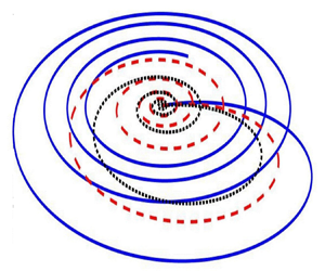
It is known that an Ekman spiral refers to wind or current structures that are developed near a horizontal boundary. As one moves away from the boundary region, the direction of the flow deviates from the external forcing and rotates gradually. Generally, the transport of volume associated with the Ekman spiral occurs in the right-hand direction towards the northern hemisphere. However, in the case of electro-osmotic flow, the Ekman spirals exhibit different characteristics. The direction of the volume transportation of electro-osmotic flow is essentially dependent on $\omega$ as depicted in figure 2. The Ekman spirals obtained in this scenario are observed as closed curves, and as the value of $\omega$ increases, the area enclosed by the curves tends to decrease. Notably, each closed curve originates from the origin ($z=0$). As $z$ increases, the $u$-component swirls along the positive $x$-axis, while the component $v$ swirls along the negative $y$-axis. When $u$ reaches its maximum value, the spiral changes direction until the $-v$ velocity reaches its maximum. Following this, the magnitudes of both $u$ and $v$ begin to decrease, eventually spiraling back towards the origin as witnessed in figure 2.

Figure 2. When considering a single plate, the Ekman spirals exhibit different closed spirals in the steady state corresponding to different values of $\omega$. Regardless of the value of $\omega$, closed spirals are obtained consistently. However, as the value of $\omega$ increases, the area enclosed by these spirals gradually shrinks in size.

We rewrite (3.7) and (3.10) as

(3.17)\begin{equation} \psi^{\prime\prime}+p\psi^{\prime}-q\psi=0 \end{equation}

and

(3.18)\begin{equation} \chi^{\prime\prime}+p\chi^{\prime}+m^{2}\chi+\psi=0, \end{equation}

where $q=\alpha ^2+1$. Equations (3.17) and (3.18) along with the boundary conditions (3.11a,b) and (3.12a,b) are solved using Galerkin approximation. We approximate the functions $\chi (z)$ and $\psi (z)$ by a finite series that can be obtained from a complete continuous set of linearly independent functions $\chi _n(z)$ and $\psi _n(z)$. The functions are approximated in such a way that they satisfy the boundary conditions. We take the following approximations for $\chi$ and $\psi$:

(3.19)\begin{equation} \left.\begin{gathered} \chi(z)=\sum_{n=1}^{N} a_n\,\chi_n(z), \\ \psi(z)=\sum_{n=1}^{N} b_n\,\psi_n(z), \end{gathered}\right\} \end{equation}

where $a_n$ and $b_n$ are constants. For the sake of mathematical simplicity, we consider $n=2$ and the following basis functions for $\chi _n(z)$ and $\psi _n(z)$:

(3.20a,b)\begin{equation} \chi_1(z)=z\,{\rm e}^{{-}z}, \quad \chi_2(z)=z^2\,{\rm e}^{{-}z}, \end{equation}

and

(3.21a,b)\begin{equation} \psi_1(z)={\rm e}^{{-}z}, \quad \psi_2(z)={\rm e}^{{-}2z}. \end{equation}

The relevant equations (3.20a,b) and (3.21a,b) are substituted in (3.17) and (3.18). The residuals are obtained in each case. The sets of coefficients $a_n$ and $b_n$ are determined using the fact that each residual is orthogonal to the set of trial functions over the selected domain. The integral formulation can be written as

(3.22a,b)\begin{equation} \int_{0}^{\infty}\chi_n (z)\,R_1 \,{\rm d}z=0 \quad \mbox{and} \quad \int_{0}^{\infty}\psi_n(z)\,R_2 \,{\rm d}z=0 \quad (n=1,2), \end{equation}

where $R_1$ and $R_2$ are the respective residues. Equations (3.22a,b) lead to a homogeneous system of linear equations with four unknowns. The necessary condition for the existence of a non-trivial solution gives rise to the approximated equation

(3.23)\begin{align} &0.0016(1.6+m^4+1.32\alpha^2-5.33\beta+5.33\alpha^2+10.66{\rm i}\omega +4{\rm i}\alpha\beta-4{\rm i}\alpha^3+8\alpha\omega)\nonumber\\ &\quad{}\times (\beta-\alpha^2-2{\rm i}\omega-2.5\alpha^2+0.5\alpha^4-3{\rm i}\alpha+3{\rm i}\alpha^3)=0. \end{align}

This equation is solved numerically to obtain the values of $\alpha$ for which the flow is either stable or unstable. Consequently, the nature of the Ekman spirals is analysed in the stable and unstable regions.

Case B: we analyse Ekman spirals in unstable and stable regions.

In the unstable region, the Ekman spirals are closed curves that initiate from the origin. In the unstable region, as the value of $\omega$ increases in the range $\omega <1$, the area enclosed by the Ekman spirals also increases, and the spirals gradually shift towards the left.

On the other hand, when $\omega > 1$, the Ekman spirals continue to shift towards the left as the value of $\omega$ increases. However, the area enclosed by the spirals becomes smaller with increasing values of $\omega$. The maximum enclosed area is obtained at $\omega =1$. By comparing figures 3(a) and 3(b), it is apparent that the deviation of the Ekman spirals in the leftward direction is considerably smaller for $\omega \geq 1$ compared to $\omega <1$.

Figure 3. Unstable Ekman spirals: (a) when $\omega \leq 1$, (b) when $\omega >1$. Closed Ekman spirals initiating from the origin are obtained in unstable cases as well. The deviation of the spirals towards the left is substantially smaller when $\omega >1$ compared to when $\omega \leq 1$.

In the stable region (when $\textrm {Re}(\beta )>0$), the behaviour of the Ekman spirals differs from that in the unstable region, as can be seen in figure 4. In the stable region, the Ekman spirals appear as broken curves that initiate from the origin. As the value of $\omega$ increases, the discontinuity or ‘cut’ present in the broken spiral gradually diminishes, but a closed curve is never formed. Additionally, with an increasing value of $\omega$, the area covered by the curve also reduces, and finally, the discontinuity or ‘cut’ in the spiral moves closer to the origin. As $\omega \rightarrow \infty$, both axial and lateral electro-osmotic flow velocities become negligible. This observation indicates that as $\omega \rightarrow \infty$, the system behaves like a rigid body, where the fluid motion becomes significantly restricted.

Figure 4. In the case of stable flow, the Ekman spirals are broken curves with the origin as the initiation point. (a) A prominent discontinuity is observed for smaller values of $\omega$. (b) As $\omega$ increases, the discontinuity in each Ekman spiral diminishes. For $\omega =1$, the discontinuity in the Ekman spiral is shown in an inset.

3.1.5. Physical significance of the Ekman spirals

We introduce the rotational parameter $\omega$, defined as the ratio of the Reynolds number $Re$ to the Rossby number $Ro$. A small Rossby number $Ro$ indicates a strong Coriolis force. Given the relationship $\omega ={Re}/{Ro}$, the influence of the Coriolis force becomes more dominant compared to the viscous force of the fluid with the increasing values of $\omega$ in the regime $\omega >1$. Consequently, the Ekman spirals become more tightly confined and shrink in size with increasing $\omega$. Conversely, $\omega <1$ signifies a weaker Coriolis force, and in this regime, the viscous force predominates, resulting in disorganized and shifting spiral patterns. However, in the case of stable flow, where perturbations and disturbances have reduced impact, the Ekman spirals align almost perfectly, as depicted in figure 4.

The Ekman spiral curves obtained in both stable and unstable regions hold physical significance, as the curves arise due to the Coriolis effect. The distinction between ‘complete’ and ‘broken’ Ekman spirals reflects the persistence or decay of disturbances developed owing to the Coriolis force. In the unstable region, the closed curves of the Ekman spirals suggest that the disturbances developed by the Coriolis effect persist indefinitely and spiral along the closed curves. This implies that the influence of the Coriolis force continues to shape the flow patterns in the unstable region. In the stable region, it is observed from figure 4 that the Ekman spirals do not form closed curves and consist of a discontinuity or ‘cut’ near the origin. The extent of discontinuity, equivalently opening of the ‘cut’, reduces in size with the increasing value of $\omega$, as illustrated in figures 4(a) and 4(b). This observation signifies that as the value of $\omega$ increases, the disturbance being developed also increases. Consequently, the ‘cut’ opening decreases, implying that the disturbances die out beyond a certain period of time.

3.2.1. Linear stability analysis

We assume that the normal mode solutions to (3.25), (3.26) and (3.27) are taken in the form

(3.28)\begin{equation} \begin{bmatrix} u(z,t)\\ v(z,t)\\ \psi(z,t) \end{bmatrix} = \begin{bmatrix} \hat{u}(z) \\ \hat{v}(z) \\ \hat{\psi}(z) \end{bmatrix} \exp({{\rm i} \alpha z-\beta t}), \end{equation}

where $\alpha$ is the wavenumber along the $z$-direction and $\beta$ is the growth rate (which can be a complex quantity). Substituting these modes into (3.25), (3.26) and (3.27), and considering $\chi = \hat {u}+\textrm {i} \hat {v}$, we obtain the equations

(3.29)\begin{equation} \chi'' +a\chi'+b\chi +K^{2}\psi=0 \end{equation}

and

(3.30)\begin{equation} \psi''+a\psi'-L\psi=0. \end{equation}

The corresponding boundary conditions are defined as

(3.31a,b)\begin{equation} \chi(\pm1)=0\quad \mbox{and}\quad \psi(\pm1)=1, \end{equation}

where $a=2\textrm {i}\alpha$, $b=\beta -\alpha ^2-2\textrm {i}\omega$ and $L=K^2+\alpha ^2$, and we rewrite $\hat {\psi }$ as $\psi$ by dropping the hat symbol.

The relevant equations (3.29) and (3.30), along with the boundary conditions (3.31a,b), are solved using a Galerkin approximation method as adopted in Reza & Gupta (Reference Reza and Gupta2012) and Shivakumara et al. (Reference Shivakumara, Lee, Vajravelu and Akkanagamma2012). The functions $\chi (z)$ and $\psi (z)$ are approximated by a finite series obtained from a complete continuous set of linearly independent functions $\chi _n(z)$ and $\psi _n(z)$. We take the following approximate solutions for $\chi$ and $\psi$:

(3.32)\begin{equation} \left.\begin{gathered} \chi(z)= \sum_{n=1}^{n=N} a_{n}\,\chi_{n}(z), \\ \psi(z)= \sum_{n=1}^{n=N} b_{n}\,\psi_{n}(z), \end{gathered}\right\} \end{equation}

where $a_n$ and $b_n$ are constants, and $\chi _n(z)$ and $\psi _n(z)$ denote the sets of basis functions satisfying the respective boundary conditions. We choose

(3.33a,b)\begin{equation} \chi_{1}(z)= z(1-z^2), \quad \chi_{2}(z)=(1-z^2)^{2} \end{equation}

and

(3.34a,b)\begin{equation} \psi_1(z)=z^4 , \quad \psi_2(z)=z^2. \end{equation}

On substituting the approximated solutions (3.33a,b) and (3.33a,b) into (3.29) and (3.30), residuals are obtained in each case. The sets of coefficients $a_n$ and $b_n$ can be obtained by using the fact that each residual is orthogonal to the set of trial functions over the selected domain. The integral formulation of the Galerkin approximation for $\chi _n (z)$ and $\psi _n (z)$ can be written as

(3.35)\begin{equation} \int_{{-}1}^{1}\chi_{n}(z)\,R_1\,{\rm d}z=0, \quad n=1,2, \end{equation}

and

(3.36)\begin{equation} \int_{{-}1}^{1}\psi_{n}(z)\,R_2\,{\rm d}z=0 ,\quad n=1,2, \end{equation}

where $R_1$ and $R_2$ are the respective residues.

Equations (3.35) and (3.36) lead to a homogeneous system of linear equations in four unknowns. The necessary condition for the existence of a non-trivial solution gives rise to

(3.37)\begin{equation} \begin{vmatrix} -1.6+0.152b & -0.609a & 0 & 0 \\ 0.609a & 0.812b-2.438 & 0.051K^2 & 0.152K^2 \\ 0 & 0 & 3.428-0.222L & -0.285L+0.8\\ 0 & 0 & 4.8-0.285L & 1.33-0.4L\\ \end{vmatrix} =0. \end{equation}

On expanding (3.37), we obtain the following approximated biquadratic equation in $K$ as

(3.38)\begin{align} &L^2(0.0295+0.0028a^2-0.0126b+0.0009b^2)-L(0.2673+0.0249a^2-0.1123b+0.008b^2) \nonumber\\ &\quad +(2.76411+0.2628a^2-1.1832b+0.0874b^2)=0, \end{align}

where $K$ is the dimensionless electrokinetic width, $a=2\textrm {i}\alpha$, $b=\beta -\alpha ^2-2\textrm {i}\omega$ and $L=K^2+\alpha ^2$. Equation (3.38) consists of both real and imaginary parts. However, the physical definition of $K$ requires that $K$ must be real. Hence the solution of (3.38) for a fixed value of $\omega$ is considered by taking the absolute value of $K$. This consideration is valid because in (3.29), $\chi =\hat {u}+\textrm {i} \hat {v}$ represents complex velocity potential. The plot of $|K|$ versus $\alpha$, as depicted in figure 5(a), illustrates the neutral stability curve with respect to the parameter $K$ for the complex velocity potential. As $\beta =\beta _{r}+\textrm {i}\beta _{i}$, we consider the case of direct bifurcation when $\beta _r=\beta _i=0$. In this situation, (3.38) can be solved to get the neutral curve with respect to the parameter $K$ for complex velocity potential with different values of $\omega$. From figure 5(a), we observe that with an increase in $\omega$, the regions of both stable and unstable zones change significantly. To ascertain the accuracy of our results, we conducted analyses using one, two and three basis functions within the Galerkin expansion framework. Our findings indicate that the outcomes derived from employing two and three basis functions are closely aligned. However, as witnessed in figure 5(b), there is a noticeable discrepancy in the results when considering only a singular term in the Galerkin approximation. A comparative illustration of these results is presented in figure 5(b). While the inclusion of three basis functions provides rigorous insights, the associated computational complexities prompted us to utilize a more streamlined approach with two basis functions for the present analysis.

Figure 5. (a) Neutral stability curve for $K$ versus $\alpha$ with different values of $\omega$. The neutral stability curve separates the regions of stability and instability of fluid flow. In this illustration, the stable region exhibits on the lower side of each neutral stability curve, while the upper side corresponds to the unstable region. As the value of $\omega$ increases, the instability region increases. (b) Comparison of the numerical results by taking a singular-term Galerkin approximation, a two-point Galerkin approximation and a three-point Galerkin approximation when $\omega =10$.

Figures 6(a) and 6(b) plot the variation of real growth rate $\beta _r$ versus wavenumber $\alpha$ for different values of $K$, obtained at $\omega =1$ and $10$, respectively. It is worth mentioning that pertaining to the case $\omega =1$, no instability is observed for $K=1.5$. This observed behaviour can be attributed to a relatively lower strength of rotational forcing for $\omega =1$ together with a significantly smaller electrokinetic parameter at $K=1.5$. However, as the value of $K$ increases, the channel width also increases, leading to the emergence of instabilities beyond a critical wavenumber. The critical wavenumber, which corresponds to a zero growth rate, can be calculated by identifying the value of $\alpha$ at which the growth rate becomes zero, as indicated by the curve. As witnessed in figures 6(a) and 6(b), for $\omega =1$ and higher values of $K$, the flow remains stable for smaller values of $\alpha$. However, instabilities start to manifest as the wavenumber increases. These inferences suggest that the stability of the underlying flow is influenced by the rotation parameter ($\omega$) and the electrokinetic width ($K$), leading to a wider range of wavenumbers implicating the onset of instabilities.

Figure 6. Variation of real growth rate $\beta _r$ versus $\alpha$ and transition from stability to instability. (a) Different values of $K$ when $\omega =1$. When $K=1.5$ and $\omega =1$, the flow is always stable. This trend of stable flow for $K=1.5$ continues for a value of $\omega$ taken roughly up to 5.95. (b) Different values of $K$ when $\omega =10$. When $K$ is small, there is a transition towards stability from instability. However, as $K$ is increased, the flow gradually transits to an unstable flow from a stable flow.

In the analysis dealing with the transition to instability with a fixed value of $K$ and for different values of $\omega$ as depicted in figures 6(a) and 6(b), we observe that for $K=1.5$, the flow remains stable for $\omega =1$. It can also be shown (as elaborated later) that for $K=1.5$, the flow remains stable for $\omega \approx 5.95$. This is also depicted in figure 7(a). However, instabilities start to emerge as $\omega$ increases beyond its critical value ($\omega \geq 6$). These instabilities gradually lead to stability as the wavenumber increases. This observation suggests a transition from stability to instability as $\omega$ exceeds a critical value. The exact critical value of $\omega$ depends specifically on the problem under consideration.

Figure 7. Variation of real growth rate $\beta _r$ versus $\alpha$ and transition from stability to instability. (a) Different values of $\omega$ when $K=1.5$. For significantly small values of $K$, the flow gradually tends to be stable with increasing wavenumber. (b) Different values of $\omega$ when $K=10$. For large values of $K$, the flow is stable only for smaller wavenumbers, while the instabilities occur in the flow as the wavenumber increases.

Figure 7(b) shows different trends of the stability picture for the higher values of $\omega$ considered. At a higher value of $\omega \ (=10)$, the flow is stable only for smaller wavenumber $\alpha$. Increasing the value of $\alpha$, the flow gradually becomes unstable, as witnessed by the growth rate curve for different values of $K$ in the figure.

We rewrite (3.38) in the form

(3.39)\begin{equation} AK^4-BK^2+C=0, \end{equation}

where $A$, $B$ and $C$ are defined in Appendix A.

We seek to find the critical wavenumber above which instabilities appear in the flow corresponding to the different values of $K$ and $\omega$. We put $\beta =0$ in (3.39), and perform an implicit derivative of $K$ with respect to $\alpha ^2$. Thus the rate of change of $K$ with respect to $\alpha ^2$ is obtained as

(3.40)\begin{equation} \frac{{\rm d}K}{{\rm d}\alpha^2}= \frac{\varLambda K^4+K^2(2\alpha^2\varLambda+2\delta-\varGamma)+(\alpha^4\varLambda+2\delta\alpha^2-\alpha^2\varGamma-\xi+\epsilon)}{4K^3\delta+2\tau K}, \end{equation}

where $\tau,\delta,\varLambda, \varGamma, \xi,\varGamma$ are defined in Appendix A. In order to find the critical wavenumber $\alpha _c$, ${\textrm {d}K}/{\textrm {d}\alpha ^2}$ is set to zero. As a result, we obtain

(3.41)\begin{equation} \varLambda K^4+K^2(2\alpha_c^2\varLambda+2\delta-\varGamma)+(\alpha_c^4\varLambda+2\delta\alpha_c^2-\alpha_c^2\varGamma-\xi+\epsilon)=0. \end{equation}

This equation is solved numerically for different values of $\omega$ after substituting the value of $K$ from (3.39). It is to be noted that since wavenumber is a real quantity, only the real part of $\alpha _c$ is to be considered from the solution obtained from (3.41). Finally, the critical wavenumber above which the instabilities appear in the flow can be obtained for different values of $K$ and $\omega$.

In order to study the variation of $K_c$ (critical electro-osmotic parameter) with respect to wavenumber, the reciprocal of (3.40) is set to zero. The expression of $K_c$ for different values of $\omega$ as a function of $\alpha$ is thus obtained as

(3.42)\begin{equation} K_c= \sqrt{-\frac{\tau}{2\delta}}. \end{equation}

Figure 8(a) represents the variation of critical wavenumber ($\alpha _c$) with $K$ for different values of $\omega$. It is seen that with increasing $\omega$, the range of $\alpha _c$ increases. This shows that the system under consideration tends to become stable as $\omega$ is increased.

Figure 8. (a) Variation of critical wavenumber $\alpha _c$ with electro-osmotic parameter $K$, for different values of $\omega$. As $\omega$ increases, the critical value of $\alpha$ becomes gradually higher. (b) Variation of critical $K$ with wavenumber at different values of $\omega$.

The variation of critical electro-osmotic parameter $K_c$ with wavenumber $\alpha$ for different $\omega$ is shown in figure 8(b). It can be seen that with increasing $\alpha$, the critical electro-osmotic parameter $K_c$ first decreases and then increases with increasing $\alpha$.

3.2.2. Analytical verification: employment of the modified Routh–Hurwitz criterion

Here, we make an effort to verify the stability threshold of the flow field, employing an analytical method consistent with the modified Routh–Hurwitz criterion. Using this method, we check the stability of the flow for $K=1.5$ and in the neighbourhood of $\omega =5.9$. Additionally, we establish by using this method that the flow is always stable for $K=1.5$ and $\omega \approx 5.95$. The Routh–Hurwitz criterion is a method used to determine whether the real part of a root of an equation is positive or negative. This technique allows us to determine the sign of the real part of the root without solving the equation (D'Azzo & Houpis Reference D'Azzo and Houpis1960; Anagnost & Desoer Reference Anagnost and Desoer1991). However, when the equation contains complex coefficients, the standard Routh–Hurwitz criterion is not applicable directly. In such cases, the modified Routh–Hurwitz criterion is employed to analyse the stability of the system (Lung Reference Lung1966).

Equation (3.38) in terms of $\beta$ can be expressed as

(3.43)\begin{equation} P(\beta)= p\beta^2 -\beta(q+{\rm i} r)+(x+{\rm i} y), \end{equation}

where the terms $p,q,r, x,y$ are given in Appendix B. In order to apply the modified Routh–Hurwitz criterion, we introduce another polynomial ${\bar P}({\beta })$, which is the complex conjugate of the polynomial $P(\beta )$ defined in (3.43). Multiplying (3.43) by its conjugate ${\bar P}({\beta })$, we obtain the polynomial

(3.44)\begin{equation} F(\beta)=p^2\beta^4-2pq\beta^3+\beta^2\{2px+(q^2+r^2)\}-\beta(2qx+2ry)+(x^2+y^2). \end{equation}

As is evident from this equation, the zeros of the above biquadratic polynomial are complex. To determine the nature of the real part of $\beta$, which determines the stability of the flow, we construct the Routhian table using (3.44).

The number of sign changes in the first column of the Routhian table corresponds to the number of roots with a positive real part. It is important to note that the number of roots having a positive real part in (3.43) is half the numbers obtained from (3.44).

Using the modified Routh–Hurwitz criterion, we now show that the flow is always stable for $K=1.5$ and $\omega =5.9$. If we put $K=1.5$, $\omega =5.9$ in (3.43), then we obtain the polynomial

(3.45)\begin{equation} P_{1.5,5.9}(\beta)= 0.1105\beta^2-\beta(q_1+{\rm i}r_1)+(x_1+{\rm i}y_1), \end{equation}

where $q_1=1.00028+0.211\alpha ^2$, $r_1=1.5445$, $x_1=-2.0301+2.1087\alpha ^2+0.1106\alpha ^4$ and $y_1= 11.8063+2.6091\alpha ^2$.

As mentioned earlier, we introduce another polynomial $\overline {P_{1.5,5.9}}(\beta )$, which is the conjugate of ${P_{1.5,5.9}(\beta )}$, and multiply them to get the resultant biquadratic polynomial

(3.46)\begin{align} F_{1.5,5.9}(\beta)&=0.0122\beta^4-0.221q_1\beta^3+(0.221x+q_{1}^2+r_{1}^2)\beta^2 \nonumber\\ &\quad -(2y_1r_1+2q_1x_1)\beta +(x_{1}^2+y_{1}^2). \end{align}

Using (3.46), we construct the Routhian table (see table 1a) for $F_{1.5,5.9}(\beta )$.

Table 1. (a) Routhian table for $F_{1.5,5.9}(\beta )$. (b) Estimation of $A_{1}$, $A_{2}$, $B_{1}$ and $C_{1}$.

The expressions $A_1$, $A_2$, $B_1$ and $C_1$ in table 1(a) are defined in Appendix C.

Based on the analysis of data given in the Routhian table, the values of $A_1, A_2, B_1, C_1$ are obtained for $\alpha =0$–$5$ as given in table 1(b).

By comparing table 1(b) with table 1(a), it is observed that in the Routhian table, there are four changes in sign along the first column. This indicates that the complex polynomial given in (3.46) will have four zeros with a positive real part. This feature, in turn, shows that the polynomial (3.45) will have two zeros whose real part is positive. Since a positive real $\beta$ denotes a stable flow, it can be inferred that for $K=1.5$ and $\omega =6$, the flow is indeed stable.

Now we aim to show the instabilities in the flow when $K=1.5$ and $\omega =6$. We put $K=1.5$ and $\omega =6$ in (3.43), yielding the polynomial

(3.47)\begin{equation} P_{1.5,6}(\beta)=0.1105\beta^2-\beta(g+{\rm i} h)+(m+{\rm i} n), \end{equation}

where $g=1.00028+0.2211\alpha ^2$, $h=1.57065$, $m=-2.1793+2.2310\alpha ^2+0.1105\alpha ^4$ and $n=12+2.6533\alpha ^2$. By introducing the conjugate polynomial, as discussed earlier, and multiplying it with (3.47), we obtain the biquadratic polynomial

(3.48)\begin{align} F_{1.5,6}(\beta)= 0.0122\beta^4-0.221\beta^3g+(0.221m+g^2+h^2)\beta^2-(2gm+2hn)\beta+(m^2+n^2). \end{align}

In the Routhian table 2, the expressions for $A_1, A_2, B_1, C_1$ are the same as defined in table 1.

Table 2. Routhian table for $F_{1.5,6}$($\beta$).

By constructing a table similar to tables 1(a) and 1(b), and performing an analysis using tabulated data, it is observed that for $\alpha$ in the range 0–0.235, there are two sign changes. This indicates that two zeros of the polynomial (3.48) with a negative real part exist. Consequently, the polynomial (3.47) has one zero whose real part is negative. Therefore, it can be concluded that for $K=1.5$ and $\omega =6$, instabilities start to appear in the flow field.

Similarly, using the modified Routh–Hurwitz criterion for different values of $K$ and $\omega$, different ranges of wavenumbers can be obtained at which the flow is unstable.

3.2.3. Generalized flow analysis

Pertaining to the flow in a bounded configuration, we also attempt to demonstrate the flow field as described by the velocity variation in both stable and unstable scenarios. Using (3.25), (3.26) and (3.27), we obtain the differential equation in $\chi$ as

(3.49)\begin{equation} \chi''+a\chi'+b\chi={-}\frac{K^{2}\cosh\{({\rm i}\alpha+K)z\}}{\cosh({\rm i}\alpha+K)}, \end{equation}

where $a=2\textrm {i} \alpha$ and $b=\beta -\alpha ^{2}-2\textrm {i}\omega$. The right-hand side of (3.49) is obtained from the analytical solution of (3.25), subject to the boundary conditions of $\psi$ given in (3.31a,b).

The solution of (3.49) using the boundary condition (3.31a,b) takes the form

(3.50)\begin{equation} \chi(z)=\frac{{\rm e}^{{\rm i}\alpha}\,K^{2}}{K^{2}-aK+b}\left(\frac{\cosh(lz)}{\cosh l}-\frac{\cosh\{({\rm i}\alpha+K)z\}}{ \cosh ({\rm i}\alpha+K)}\right) , \end{equation}

where $l=\sqrt {2\textrm {i}\omega -\beta }$. In particular, the solution for $\alpha =0$ and $\beta =0$ reproduces the steady-state solution given by

(3.51) \begin{equation} \chi(z)=\frac{K^{2}}{K^{2}-2{\rm i}\omega} \Bigg(\frac{\cosh(\sqrt{2i\omega}\,z)}{\cosh \sqrt{2{\rm i}\omega}}-\frac{\cosh(Kz)}{\cosh K}\Bigg) . \end{equation}

It is worth mentioning here that the solution described in (3.27) aligns with the findings presented in Chang & Wang (Reference Chang and Wang2011). Specifically, for small values of $K$, the EDL potential reaches a minimum at the centre of the channel. When the value of $K$ is low, the velocity profile of $u$ is approximately parabolic in the absence of rotation, and decreases rapidly with rotation. These observations indicate the influence of rotation on the EDL potential and velocity distribution.

3.2.4. Flow characteristics at stable and unstable regions

The stability of the flow can be assessed by examining the growth rate $\beta$. A positive value of $\beta$ indicates stability, while a negative value signifies flow instability. From figure 9, we observe that the flow is always stable for $K=1.5$, $\omega =1$, hence a fully developed parabolic nature of the velocity profile is obtained. It is also seen that as the wavenumber $\alpha$ and the corresponding growth rate increase, the absolute value of the complex velocity reduces. We have performed full-scale numerical simulations using the finite element framework of COMSOL Multiphysics by considering the Poisson–Boltzmann equation with Gouy–Chapman theory for the description of EDL potential, and the Navier–Stokes equations for a purely electro-osmotically driven flow in a rotating microchannel. The comparison analysis of our results, both analytical solutions and simulated data, with the reported results of Chang & Wang (Reference Chang and Wang2011) is presented in figure 10(a). As witnessed in figure 10(a), our analytical solutions agree well with both full-scale simulated and reported theoretical results for all the values of $K$ and $\omega$ considered. In figure 10(b), we compare our analytical solutions with the experimental results of Hsieh et al. (Reference Hsieh, Lin and Lin2006) in the limiting case of a non-rotating channel. It is worth mentioning here that the lack of experimental data pertaining to rotating electro-osmotic flows encouraged us to focus on this benchmarking analysis in the limiting case. The velocity profile in the stability regions is known to expose a fully developed parabolic or wave-like structure. Conversely, in the unstable region, the flow profile takes the form of a flattened parabolic profile as depicted in figure 11(a). Figure 11(a) illustrates the variation of the resultant velocity profile at different stability conditions when the other parameters are $K=1.5$ and $\omega =10$, while 11(b) illustrates the resultant velocity profile for $K=20$ and $\omega =1$ at different stability conditions. As the value of $\beta$ increases, the velocity profiles show a plateau-like structure. The disturbance of the flow field occurs near the central line of the channel. For a set of parametric values, i.e. for $K=1.5$, $\omega =10$, both least stable and unstable zones exist. The approximate highest negative value of $\beta$ represents the most unstable velocity profile, while the least stable corresponds to the least positive value of $\beta$. The most unstable, as well as least stable, growth rate and its corresponding wavenumbers can be determined from figures 7(a) and 7(b).

Figure 9. Stable velocity profile of the resultant velocity $|\chi (z)|=\sqrt {(u^2+v^2)}$ at different wavenumbers and their corresponding growth rate: (I) $\alpha =0.08$, $\beta =2.8$; (II) $\alpha =1.51$, $\beta =6.37$; (III) $\alpha =2.48$, $\beta =10.59$, when $\omega =1$, $K=1.5$.

Figure 10. (a) Comparison of axial velocity profiles obtained from the analytical solution at the steady state (when $\alpha =0$, $\beta =0$) with direct numerical simulation and previous theoretical investigation. (b) Comparison of the present dimensional axial electro-osmotic flow velocity for the limiting case of zero rotational speed with the experimental results of Hsieh, Lin & Lin (Reference Hsieh, Lin and Lin2006) when electro-osmotic mobility is $4.21\times 10^{-8}\ \textrm {m}^2\ (\textrm {V}-\textrm {s})^{-1}$ $\textrm {m}^2/\textrm {V}/\textrm {s}$ and zeta potential is $-55.32\ \textrm {mV}$ for $10\ \textrm {mM}$ NaCl solution. The dimensional axial velocity is obtained by multiplying the electro-osmotic mobility and electric field into the present dimensionless axial velocity field for the limiting case of zero rotational speed.

Figure 11. (a) Velocity profile for the electro-osmotic flow $|\chi |=\sqrt {(u^2+v^2)}$ for $K=1.5$, $\omega =10$ when the flow is: maximum unstable ($\alpha =0.005$, $\beta =-1.613$), least stable ($\alpha =0.934$, $\beta =0.0005$) and stable ($\alpha =2.768$, $\beta =12$). (b) Velocity profile for the electro-osmotic flow $|\chi |=\sqrt {(u^2+v^2)}$ for most stable, neutral and unstable regimes when $K=20$, $\omega =1$. Here, most stable is defined as a stability of flow with maximum positive growth rate.

These profiles bear significant information about the transition of the field for electro-osmotic flow. This flattening effect can be attributed to the destabilizing factors in the flowing fluid. In the case of instability, the flow velocity profile exhibits a depression or disturbance in the vicinity of the central line of the channel. This depression signifies the disruptive effects of instability on the behaviour of the electro-osmotic flow. This characteristic feature suggests that the flow becomes more turbulent or irregular, deviating from the expected parabolic or wavy shape as demonstrated in stable conditions.