


1. Introduction
Snap-through is a buckling instability of slender bodies that drives a sudden jump between two different configurations (Holmes & Crosby Reference Holmes and Crosby2007; Gomez, Moulton & Vella Reference Gomez, Moulton and Vella2017a; Holmes Reference Holmes2019; Jiao & Liu Reference Jiao and Liu2021). In the past decade or so, this bi-stability has been recognized as a key factor in the behaviour of several biological systems. For example, the leaf lobes of the Venus flytrap exploit snap-through to efficiently catch a prey (Sachse et al. Reference Sachse, Westermeier, Mylo, Nadasdi, Bischoff, Speck and Poppinga2020), and the lower jaw of the hummingbird can execute a controlled snap that enables the bird to react sufficiently rapidly to catch a flying insect (Smith, Yanega & Ruina Reference Smith, Yanega and Ruina2011). Technological applications exploit the snap-through instability in the design of mechanical switches (Schultz & Hyer Reference Schultz and Hyer2003; Giannopoulos, Monreal & Vantomme Reference Giannopoulos, Monreal and Vantomme2007; Rothemund et al. Reference Rothemund, Ainla, Belding, Preston, Kurihara, Suo and Whitesides2018; Preston et al. Reference Preston, Jiang, Sanchez, Rothemund, Rawson, Nemitz, Lee, Suo, Walsh and Whitesides2019a,Reference Preston, Rothemund, Jiang, Nemitz, Rawson, Suo and Whitesidesb), small-scale pumps (Li et al. Reference Li, Wang, Foo, Godaba, Zhu and Yap2017) and energy-harvesting devices (Zhao & Suo Reference Zhao and Suo2010; Harne & Wang Reference Harne and Wang2013). In the biomedical engineering industry, snap-through has been exploited in the design of artificial heart valves that enable a rapid and reversible response to an external stimulus, such as a change in hydraulic pressure from blood vessels (Gonçalves et al. Reference Gonçalves, Pamplona, Teixeira, Jerusalmi, Cestari and Leirner2003; Hu & Burgueño Reference Hu and Burgueño2015).
Snap instability can be actuated in various ways, including the application of a point force (Pandey et al. Reference Pandey, Moulton, Vella and Holmes2014) or the utilization of electrostatic and capillary forces (Krylov et al. Reference Krylov, Ilic, Schreiber, Seretensky and Craighead2008; Fargette, Neukirch & Antkowiak Reference Fargette, Neukirch and Antkowiak2014) or thermal effects (Boisseau et al. Reference Boisseau, Despesse, Monfray, Puscasu and Skotnicki2013; Kessler et al. Reference Kessler, Ilic, Krylov and Liberzon2018). These actuation methods drive a system towards a marginal stability state, from which only a small perturbation will drive the instability. In addition to the above-mentioned mechanisms, previous studies have also explored the possibility of inducing a snap instability through incoming flows. For example, Gomez, Moulton & Vella (Reference Gomez, Moulton and Vella2017b) demonstrated a method for controlling the flow rate of a viscous fluid in a tunnel by incorporating a slender beam along the sidewall of the tunnel. They found that when the flow rate exceeded a critical value, the beam snapped out, increasing the cross-sectional area of the tunnel, and thereby controlled the flow. Arena et al. (Reference Arena, Groh, Brinkmeyer, Theunissen, Weaver and Pirrera2017) proposed an adaptive slender structure that can induce a controlled snap in response to the pressure field exerted by a surrounding fluid. Kim et al. (Reference Kim, Zhou, Kim and Oh2020, Reference Kim, Lahooti, Kim and Kim2021) revealed a mechanism of periodic snap-through in a thin sheet that was initiated by a uniform incoming flow. This mechanism was subsequently utilized to improve the performance of renewable energy-harvesting systems. Finally, Peretz et al. (Reference Peretz, Mishra, Shepherd and Gat2020) introduced an innovative approach for controlling the shape of a continuous multi-stable structure by utilizing an inlet flow as an actuation mechanism. This last technology holds promise for a range of applications, including soft robotics, biomedical devices and active materials.
Although the examples cited above demonstrate scenarios in which fluid motion triggers an elastic instability, there are also configurations in which the onset of an elastic instability drives a fluid's motion, a phenomenon that we denote as snap-induced flow. Indeed, any object that snaps and is surrounded by a fluid will interact with the fluid to some extent during its motion. The measure of interaction between the snapping object and its surrounding fluid can vary, depending on several factors, including the properties of both the fluid and the object and the geometry of the object. For instance, the snap-through of the Venus flytrap is affected only minimally by the surrounding air, because the ratio of hydrodynamic to elastic forces is relatively small (Forterre et al. Reference Forterre, Skotheim, Dumais and Mahadevan2005). In contrast, the snapping of a shrimp's claw interacts strongly with the surrounding water. The resulting high-pressure water jet from the snap can stun or even kill a prey (Versluis et al. Reference Versluis, Schmitz, von der Heydt and Lohse2000; Tang & Staack Reference Tang and Staack2019). Another example is that of microfluidic pumps, which use snap-induced flow to drive the motion of the fluid within the microchannels (Tavakol et al. Reference Tavakol, Bozlar, Punckt, Froehlicher, Stone, Aksay and Holmes2014).
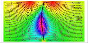
Despite the widespread occurrence of snap-induced flow in both natural and technological systems, analytical analysis of this phenomenon in the literature is relatively sparse. Our study thus aims to investigate this phenomenon by examining a representative flow generated by a snapping object. Our model consists of a closed channel that is filled with an inviscid fluid and is split into two parts by an inextensible sheet that is compressed between the sidewalls of the channel (see figure 1). Initially, the pressure difference between the upstream and downstream directions of the channel is equal to zero, and the sheet buckles towards the upstream direction. Then, the pressure difference increases slowly until the sheet loses stability and snaps. The intricate dynamics of the sheet and the fluid after snapping is examined in this article.

Figure 1. Schematic overview of the channel's cross-section in the  $\tilde {x}$–
 $\tilde {y}$ plane (the width
  $\tilde {W}$ is in the spanwise direction). A thin sheet divides a closed channel, filled with an inviscid fluid, into two parts. The pressures in the upstream and the downstream directions at a distance of
  $\tilde {L}_y/2$ from the sheet are designated
  $\tilde {P}_{{u}}$ and
  $\tilde {P}_{{d}}$, respectively.
To this end, we formulate a model that couples Kirchhoff equations, which describe the dynamics of thin sheets, with the hydrodynamics of inviscid fluids (Lamb Reference Lamb1945). In addition to the pressure difference in the channel, our model depends on three distinct dimensionless parameters: the excess length of the sheet compared with the vertical dimension of the channel,  $\varDelta$ (all the lengths are normalized to the total length of the sheet), the length of the channel,
  $L_y$, and the sheet-to-fluid mass ratio, which is represented by
  $\lambda$. We show that, although this model yields a set of complex and nonlinear equations, it can be analysed analytically in the case of small excess lengths,
  $\varDelta \ll 1$. For this purpose, we use a modal expansion of the sheet's configuration and the fluid's potential functions to derive analytical solutions that hold both at the onset of the instability and at later stages of the dynamic evolution (Goncharuk, Feldman & Oshri Reference Goncharuk, Feldman and Oshri2023).
To identify the onset of instability, we start by recalling the quasi-static evolution of the system, which encompasses different branches of solutions (for details, refer to Oshri (Reference Oshri2021)). We then conduct a linear stability analysis around the primary branch of the solutions, and calculate the growth rate of the instability ( $\sigma$) and the critical pressure difference at which the onset of instability occurs. We show that the instability primarily perturbs the sheet's configuration via an asymmetric eigenfunction. This perturbation induces a rotational pattern flow in the channel that does not lead to a net flow of fluid from the upstream direction to the downstream direction. The appearance of the net flow is shown to emerge as a higher-order correction to the theory. To analyse the weakly nonlinear stage of the system's evolution, we first show that the sheet's evolution is determined mainly by its first two modes of buckling. This allows us to simplify our set of nonlinear equations into a single and tractable equation for one of the modes. By solving this equation, we gain valuable insights into the system's evolution, including the emergence of the net flow in the channel, with an exponential growth rate of
  $2\sigma$, and the pressure difference on the sheet as a function of its geometry.
Of particular interest is the behaviour of the system when the sheet-to-fluid mass ratio is relatively small, as the hydrodynamic effect on the sheet's motion dominates in such conditions. In this case, we observe that the dynamics slows down, and the system evolves along one of the quasi-static branches of solutions whose energy is higher than that of the other branches. This implies that dynamic effects enable the system to propagate along a branch that would otherwise be unstable. We also observe the emergence of pressure spikes in the channel during the system's propagation. When the snap transition occurs, the sheet initially gains bending energy up to a critical point, beyond which it rapidly releases this energy into the flow. This process generates sharp peaks of pressure drop in the channel, the duration and maximum magnitude of which depend on the system's parameters.
The paper is structured as follows. In § 2, we start by formulating the problem and obtaining a set of equations that describe the dynamics of the sheet and the fluid. We then simplify these equations using small-amplitude approximation and modal expansion. In § 3, we focus on the early evolution of the system. First, we recall the quasi-static solution of the problem and then perform linear stability analysis. Moving on to § 4, we analyse the system's evolution at intermediate times. Here, we introduce the two-mode approximation and discuss its limitations, before investigating the onset of the net flow in the channel, the pressure drop on the sheet as a function of the volume difference in the channel and the elastohydrodynamic energetic interplay. Finally, in §§ 5 and 6, we discuss the limits of the model, and then summarize the main findings and present our conclusions.
2. Formulation of the problem
An inextensible thin sheet of total length  $\tilde {L}$, bending modulus
  $\tilde {B}$, thickness
  $\tilde {h}$ and density
  $\tilde {\rho }_{{sh}}$ is compressed between the sidewalls of a closed channel. The channel is filled with an inviscid fluid of density
  $\tilde {\rho }_{\ell }$. The height and the width of the channel's cross-section are
  $\tilde {L}_x$ and
  $\tilde {W}$, respectively. The pressures in the fluid in the upstream and downstream directions, each at a distance
  $\tilde {L}_y/2$ from the sheet, are designated
  $\tilde {P}_{{u}}$ and
  $\tilde {P}_{{d}}$, respectively (figure 1). A Cartesian coordinate system is located on the bottom edge of the sheet. In the analysis that follows, all lengths are normalized to the total length of the sheet,
  $\tilde {L}$, time is normalized to the inertial time scale of the sheet
  $\tilde {t}_{\star }=\tilde {L}^2(\tilde {\rho }_{{sh}} \tilde {h}/\tilde {B})^{1/2}$ and the pressure fields are normalized to
  $\tilde {B}/\tilde {L}^3$. In addition, all dimensional parameters are denoted with a tilde, while their non-dimensional counterparts appear without a tilde, for example,
 \begin{equation} t=\tilde{t}/\tilde{t}_{{\star}}, \quad L_x=\tilde{L}_x/\tilde{L}, \quad x=\tilde{x}/\tilde{L}, \quad P_{{u}}=\tilde{P}_{{u}}\tilde{L}^3/\tilde{B},\quad \text{etc.} \end{equation}
This implies the normalization of the hydrodynamic and elastic fields, as is further discussed below.
To initialize the system, we set the pressure difference between the upstream and downstream directions,  $P_{{ud}}\equiv P_{{u}}-P_{{d}}$, to zero. Additionally, we ensure that the sheet buckles towards the upstream direction, as shown in figure 1. Subsequently, we slowly increase the pressure difference in the channel until the sheet loses stability and snaps. At the point of instability, we reset the time to
  $t=0$ and investigate the coupled dynamics of the elastic sheet and the fluid flow for
  $t\geq 0$.
Our model is based on the following assumptions. Firstly, we assume that the system remains uniform along the spanwise direction of the channel. Therefore, we set  $W=1$ and essentially consider a two-dimensional system. Secondly, we assume that the volume occupied by the elastic sheet is negligible compared with the total volume of the channel, i.e.
  $\tilde {h} \tilde {L}/\tilde {L}_x \tilde {L}_y \ll 1$. Consequently, if we define
  $L_x L_y$ as our control volume, we have
  $v_{{u}}(t)+v_{{d}}(t)=L_x L_y$, where
  $v_{{u}}(t)$ and
  $v_{{d}}(t)$ correspond to the volumes in the upstream and the downstream parts of the control volume, respectively. Hereafter, we denote quantities related to the upstream and downstream directions of the control volume by the subscripts ‘u’ and ‘d’, respectively. Thirdly, we assume that there is no contact between the sheet and the sidewalls of the channel, or of the sheet with itself, at any time during the system's evolution. Lastly, we choose the length of the control volume,
  $L_y$, to be larger than the characteristic length scale at which the flow disturbances induced by the motion of the sheet decay to zero.
The velocity profiles and the pressure fields of an irrotational, inviscid flow are determined by four fields. The first two fields correspond to the potential functions,  $\phi _i(x,y,t)$, where
  $i=u, d$, determined in the upwards and downwards sections of the channel. From these potentials, we can determine the fluid's velocity
  ${\boldsymbol v}_i=\boldsymbol {\nabla }\phi _i$, where
  $\boldsymbol {\nabla }$ is the two-dimensional gradient operator. The remaining two fields are the pressure fields
  $p_i(x,y,t)$. Using our normalization convention, we find that the potential functions are normalized to
  $(\tilde {B}/\tilde {\rho }_{{sh}} \tilde {h})^{1/2}$. The evolutions of these hydrodynamic fields, in space and over time, are determined by the continuity and Bernoulli's equations:
 $$\begin{gather} \nabla^2 \phi_i = 0, \end{gather}$$
 $$\begin{gather}\lambda p_i+\frac{\partial \phi_i}{\partial t}+\frac{1}{2}|\boldsymbol{\nabla} \phi_i|^2 = c_i(t), \end{gather}$$
where  $c_i(t)$ are arbitrary time-dependent functions used to set a Dirichlet point on each side of the channel. In our system, the pressures in the upstream and downstream directions are predetermined by the boundary conditions at
  $y=\pm L_y/2$. Therefore, the functions
  $c_i(t)$ can take any arbitrary value as long as we satisfy these boundary conditions. For the sake of convenience, we set
  $c_i(t)=\lambda P_i$ in the following analysis. This choice explicitly implies that the pressure is a constant along each side of the channel when the fluid is at rest. In addition, we define the dimensionless parameters
 \begin{equation} \lambda=\frac{\tilde{\rho}_{{sh}}\tilde{h}}{\tilde{\rho}_{\ell}\tilde{L}}, \quad \varDelta=\frac{\tilde{L}-\tilde{L}_x}{\tilde{L}}=1-L_x, \end{equation}
where the parameter  $\lambda$ represents the sheet-to-fluid mass ratio, which takes into account the relative densities of the sheet and the fluid, and the second parameter
  $\varDelta$ accounts for the excess length of the sheet compared with the vertical dimension of the channel, i.e.
  $\tilde {\varDelta }=\tilde {L}-\tilde {L}_x$. Since we are considering an inviscid fluid, the boundary conditions on the fluid–channel interfaces correspond to no penetration. In addition, the pressures in the fluid at
  $y=\pm L_y/2$ are predetermined. These boundary conditions are given by
 $$\begin{gather} \frac{\partial \phi_i}{\partial x}(0,y,t)=\frac{\partial \phi_i}{\partial x}(1-\varDelta,y,t)=0, \end{gather}$$
 $$\begin{gather}p_i(x,\pm L_y/2,t)=P_i. \end{gather}$$
 To obtain a closed set of equations it remains to model the contact between the sheet and the fluid. To this end, we introduce the position vector to a point on the sheet  ${\boldsymbol {x}}_{{sh}}(s,t)=(x_{{sh}}(s,t),y_{{sh}}(s,t))$, where
  $s\in [0,1]$ is the normalized arclength parameter, and we define the angle
  $\theta (s,t)$ between the tangent to the sheet and the
  $x$ axis, as shown in figure 1. The elastic fields
  $x_{{sh}}(s,t)$,
  $y_{{sh}}(s,t)$ and
  $\theta (s,t)$ are not independent since they are related by the following geometric constraints:
 $$\begin{gather} \frac{\partial x_{{sh}}}{\partial s}=\cos\theta, \end{gather}$$
 $$\begin{gather}\frac{\partial y_{{sh}}}{\partial s}=\sin\theta. \end{gather}$$
Using these definitions of the elastic fields, we first ensure that there is no penetration of the fluid through the sheet interface. This requirement is satisfied by imposing kinematic constraints on each side of the sheet (see Appendix A):
 \begin{equation} y=y_{{sh}}(x,t), \quad \frac{{\rm D} y_{{sh}}}{{\rm D} t}=\frac{\partial \phi_i}{\partial y}, \end{equation}
where  ${\rm D}/{\rm D}t=\partial /\partial t +{\boldsymbol v}_i \boldsymbol{\cdot } \boldsymbol {\nabla }$ is the two-dimensional convective derivative. Second, we ensure proper transfer of the momentum between the fluid and the sheet. This requirement is satisfied by enforcing the following balance of moments and forces on the sheet:
 $$\begin{gather} \frac{\partial^2\theta}{\partial s^2} =-F_x \sin\theta+F_y \cos\theta, \end{gather}$$
 $$\begin{gather}\frac{\partial^2 x_{{sh}}}{\partial t^2} =-\frac{\partial F_x}{\partial s} -[\,p_{{d}}(x_{{sh}},y_{{sh}},t)-p_{{u}}(x_{{sh}},y_{{sh}},t)]\sin\theta, \end{gather}$$
 $$\begin{gather}\frac{\partial^2 y_{{sh}}}{\partial t^2} =-\frac{\partial F_y}{\partial s} +[\,p_{{d}}(x_{{sh}},y_{{sh}},t)-p_{{u}}(x_{{sh}},y_{{sh}},t)]\cos\theta, \end{gather}$$
where  $F_x(s,t)$ and
  $F_y(s,t)$ are the
  $x$ and
  $y$ components of the reaction forces per unit length at a cross-section of the sheet, and the pressure difference term in (2.7b) and (2.7c) is multiplied by
  $\hat {\boldsymbol {n}}_{{d}}=(-\sin \theta,\cos \theta )$, which is the unit normal vector on the sheet that points outwards from the downstream side of the channel. Equations (2.7) are supplemented by the following hinged boundary conditions on the sheet's edges:
 $$\begin{gather} x_{{sh}}(0,t)=0, \quad x_{{sh}}(1,t)= 1-\varDelta, \end{gather}$$
 $$\begin{gather}y_{{sh}}(0,t)=0, \quad y_{{sh}}(1,t)=0, \end{gather}$$
 $$\begin{gather}\frac{\partial \theta}{\partial s}(0,t)=0,\quad \frac{\partial \theta}{\partial s}(1,t)=0. \end{gather}$$
 This completes the formulation of the problem. In summary, given the excess length,  $\varDelta$, the sheet-to-fluid mass ratio,
  $\lambda$, the horizontal dimension of the channel,
  $L_y$, the pressures,
  $P_{{u}}$ and
  $P_{{d}}$, and a proper set of initial conditions, we can, in principle, solve (2.2)–(2.8) to obtain the temporal evolution of the system. While this set of equations can be solved numerically, a deeper understanding of the elastohydrodynamic interactions can be obtained by considering the limit
  $\varDelta \ll 1$, i.e. the so-called small-amplitude approximation. For this reason, in the next section we reduce our formulation to this limit and utilize it to study the system's behaviour close to the snap-through instability. A numerical solution of the more general formulation is used subsequently to validate the reduced model; see Appendix B for details of the numerical solution.
Prior to proceeding to the next section, it is useful to comment on the system's conserved quantity. Since we consider an elastic model for the sheet and an inviscid model for the fluid, the sum of the total energy of the system and the work done by the external pressures are conserved throughout the system's evolution. Indeed, following the derivations in Appendix C it can be shown that (2.2)–(2.8) have the conserved first integral
 \begin{equation} H=E(t)+P_{{ud}} v_{{d}}(t), \end{equation}
where  $P_{{ud}}=P_{{u}}-P_{{d}}$ is the pressure difference between the upstream and the downstream directions and
  $E(t)=E_{{sh}}^{k}(t)+E_{{sh}}^{p}(t)+E_{{f}}(t)$ is the total energy of the system. The total energy is comprised of three contributions: the kinetic energy of the sheet,
  $E_{{sh}}^{k}(t)=\frac {1}{2}\int _0^1 |\partial {\boldsymbol {x}}_{{sh}}/\partial t|^2\, {\rm d} s$, where
  $| \cdot |$ corresponds to the norm of the enclosed vector; the potential energy of the sheet,
  $E_{{sh}}^{p}(t)=\frac {1}{2}\int _0^1 (\partial \theta /\partial s)^2\, {\rm d} s$; and the kinetic energy of the fluid,
  $E_{{f}}(t)=\sum _{i={u,d}}({1}/{2\lambda })\iint _{v_i(t)}|\boldsymbol {\nabla }\phi _i|^2\, {\rm d}\kern0.06em x \,{{\rm d} y}$. We note that with our normalization convention it can be shown that energy is normalized to
  $\tilde {B}/\tilde {L}$.
Since the sheet and the fluid are almost at rest close to the elastic instability and the kinetic energies of the sheet and fluid are very small, the total energy of the system at  $t=0$ equals the potential energy of the sheet,
  $E(0)\simeq E_{{sh}}^{{p}}(0)$. Consequently,
  $H\simeq E_{{sh}}^{{p}}(0)+P_{{ud}}v_{{d}}(0)$ is conserved throughout the system's evolution.
2.1. The small-amplitude approximation
The assumption that the lateral displacement remains small,  $\varDelta \ll 1$, or equivalently that the amplitude of the sheet is small, implies that, to leading order, the geometric relations, (2.5), reduce to
  $\partial y_{{sh}}/\partial s\simeq \theta$ and
  $\partial x_{{sh}}/\partial s\simeq 1-\frac {1}{2}(\partial y_{{sh}}/\partial s)^2$. With these approximations, the constraint on the lateral displacement of the sheet, (2.8a), becomes
 \begin{equation} \varDelta=\frac{1}{2}\int_0^1\left(\frac{\partial y_{{sh}}}{\partial x}\right)^2\, {\rm d}\kern0.06em x, \end{equation}
where we replace the arclength coordinate of the sheet with the Eulerian coordinate of the fluid,  $s\simeq x$, according to our level of approximation. The balance of forces (see (2.7)) reduces in the small-amplitude approximation to
 \begin{equation} \frac{\partial^2 y_{{sh}}}{\partial t^2}+\frac{\partial^4 y_{{sh}}}{\partial x^4}+F_x(t)\frac{\partial^2 y_{{sh}}}{\partial x^2}+p_{{u}}(x,0,t)-p_{{d}}(x,0,t)=0, \end{equation}
where to leading order the lateral compression,  $F_x(t)$, is found to be solely a function of time.
Equations (2.10) and (2.11) describe the elastic part of the model. To complete the reduction of the model, we need to approximate the hydrodynamic equations, (2.2) and (2.6). For this purpose, we use the conserved quantity, (2.9), to estimate the order of the hydrodynamic fields. At the onset of the instability, the system is nearly at rest, and we can approximate the conserved quantity as  $H \simeq E_{{sh}}^{{p}}(0)+P_{{ud}} v_{{d}}(0)$. The potential energy of the sheet, represented by the first term in
  $H$, is proportional to
  $E_{{sh}}^{{p}}(0) \sim \varDelta$, because it scales as a square of the sheet's amplitude. Moreover, up to a constant shift in
  $H$, the second term scales approximately as
  $P_{{ud}} v_{{d}}(t) \sim \varDelta$, and this scaling holds throughout the system's evolution. This scaling arises from the subsequent analysis of the small-amplitude approximation, which reveals that both
  $P_{{ud}}$ and
  $v_{{d}}(t)$ scale proportionally to
  $\sqrt {\varDelta }$. During the dynamic evolution, the energy released from the sheet, combined with the work done by the external pressures, act to increase the fluid's velocity. However, since
  $H\sim \varDelta$ remains constant and
  $P_{{ud}} v_{{d}}(t) \sim \varDelta$, the fluid's energy must, at most, also be proportional to
  $|\boldsymbol {\nabla }\phi |^2\sim \varDelta$. Assuming that a derivative of the potential functions with respect to time or a spatial coordinate does not change this scaling, i.e.
  $\phi _i\sim \sqrt {\varDelta }$, we can simplify Bernoulli's equation, (2.2), and the kinematic boundary conditions, (2.6), to
 $$\begin{gather} p_i-P_i =-\frac{1}{\lambda}\frac{\partial\phi_i}{\partial t}, \end{gather}$$
 $$\begin{gather}\frac{\partial y_{{sh}}}{\partial t} = \left(\frac{\partial \phi_i}{\partial y}\right)_{y=0}. \end{gather}$$
These approximations are verified numerically in the following sections where we analyse the nonlinear dynamics of the system. In particular, we compare the approximated results with the numerical solution of the nonlinear model, (2.2)–(2.8). We note that since the equations of continuity, (2.2a), are already linear in the potential functions, they remain unchanged in our approximated model.
This completes the reduction of the model to the small-amplitude approximation. In summary, given the parameters  $\varDelta$,
  $L_y$,
  $P_i$ (
 $i=u, d$) and
  $\lambda$, we can obtain the system's evolution from the solution of the coupled equations (2.2a) and (2.10)–(2.12), the boundary conditions on the fluid–channel interface (2.4) and the linearized form of the boundary conditions on the sheet's edges (2.8b) and (2.8c).
We have two comments regarding this formulation. Firstly, following the derivations in Appendix D, it can be shown that the reduced model emanates from the minimization of the action  $\mathcal {S}=\int _0^T\mathcal {L}\, {\rm d} t$. Here,
  $T$ is the duration of the experiment, and the Lagrangian is given by
 \begin{align} \mathcal{L} &= \int_0^1\left[\frac{1}{2}\left(\frac{\partial y_{{sh}}}{\partial t}\right)^2-\frac{1}{2}\left(\frac{\partial^2y_{{sh}}}{\partial x^2}\right)^2+F_x(t)\left(\frac{1}{2}\left(\frac{\partial y_{{sh}}}{\partial x}\right)^2-\varDelta\right)\right. \nonumber\\ &\quad +\left.\frac{1}{\lambda}[\phi_{{d}}(x,0,t)-\phi_{{u}}(x,0,t)+\lambda t P_{{ud}}]\frac{\partial y_{{sh}}}{\partial t}\right]{{\rm d}\kern0.06em x} \nonumber\\ &\quad -\frac{1}{2\lambda}\int_{0}^{{L_y}/{2}}\int_0^1|\boldsymbol{\nabla}\phi_{{u}}|^2\, {\rm d}\kern0.06em x\, {\rm d} y-\frac{1}{2\lambda}\int_{-{L_y}/{2}}^0\int_0^1|\boldsymbol{\nabla}\phi_{{d}}|^2\, {\rm d}\kern0.06em x\, {\rm d} y, \end{align}
where the minimization is considered with respect to the elastic fields,  $y_{{sh}}(x,t)$ and
  $F_x(t)$, and the hydrodynamic fields,
  $\phi _i(x,y,t)$. Secondly, since at the far edges of the control volume,
  $y=\pm L_y/2$, the pressures in the fluid are determined by (2.4b), then from Bernoulli's equation, (2.12a), we obtain
  $\phi _i(x,\pm L_y/2,t)=0$. These boundary conditions for the potential functions are used in the minimization of the action, as is discussed further in Appendix D.
2.1.1. Modal expansion
In the small-amplitude approximation, the general solutions of the continuity equations, (2.2a), read as
 \begin{equation} \phi_i(x,y,t)=a_0^i(t)\left(y\pm \frac{L_y}{2}\right)+ \sum_{m=1}^{\infty}a_m^i(t)\cos({\rm \pi} m x)\sinh \left[{\rm \pi} m \left(\frac{L_y}{2}\pm y\right)\right]\!, \end{equation}
where  $a_m^i(t)$ (
 $m=0,1,2,\ldots$) are unknown time-dependent coefficients and the
  $\pm$ signs correspond to the solutions of the potential functions in the downstream and the upstream directions, respectively. Equation (2.14) satisfies the boundary conditions on the sidewalls of the channel, (2.4a), and the requirement that
  $\phi _i(x,\pm L_y/2,t)=0$ on the edges of the control volume. Yet, the boundary conditions on the sheet–fluid interfaces, (2.12b), are not satisfied. The unknown coefficients are later determined so as to satisfy these requirements.
Similarly, we expand the solution of the sheet's height function as follows:
 \begin{equation} y_{{sh}}(x,t)=\sum_{n=1}^{\infty}A_n(t)\sin({\rm \pi} n x), \end{equation}
where the time-dependent coefficients  $A_n(t)$ are as yet unknown. We note that this expansion automatically satisfies the boundary conditions on the sheet's edges, (2.8b) and (2.8c). We note also that while (2.15) involves infinite summation over the modes of the height function, in practice, we truncate this series at
  $n=N$. It can be shown that a closed system of equations is then obtained when the coefficients of
  $a_m^i(t)$ are truncated at
  $N-1$.
Using the two expansions for the potential functions and the sheet's height function, (2.14) and (2.15), we reduce our problem to finding the unknown coefficients,  $a_m^i(t)$ and
  $A_n(t)$, and the lateral compression force,
  $F_x(t)$, from the force balance equation, (2.11), the kinematic boundary conditions, (2.12b), and the constraint over the lateral displacement, (2.10). However, instead of using these equations directly, we take a different yet equivalent route for the solution by utilizing the action we derived earlier. To this end, we first substitute (2.14) and (2.15) in the Lagrangian, (2.13), and then integrate over the spatial coordinates. Thereafter, we minimize the action with respect to
  $a_m^i(t)$ and express these coefficients in terms of
  $A_n(t)$; see Appendix E for the details of this procedure. Overall, this gives the Lagrangian
 \begin{align}
&\mathcal{L}[A_1,\ldots,A_N,F_x]\notag\\ &\quad ={\mathsf{T}}_{nk} \frac{{\rm
d}A_n}{{\rm d}t}\frac{{\rm d}A_k}{{\rm d}t}-{\mathsf{V}}_{nk}A_nA_k
+F_x(t){\mathsf{C}}_{nk}A_nA_k-F_x(t)\varDelta+tP_{{ud}}W(n,0)\frac{{\rm
d} A_n}{{\rm d} t},
\end{align}
\begin{align}
&\mathcal{L}[A_1,\ldots,A_N,F_x]\notag\\ &\quad ={\mathsf{T}}_{nk} \frac{{\rm
d}A_n}{{\rm d}t}\frac{{\rm d}A_k}{{\rm d}t}-{\mathsf{V}}_{nk}A_nA_k
+F_x(t){\mathsf{C}}_{nk}A_nA_k-F_x(t)\varDelta+tP_{{ud}}W(n,0)\frac{{\rm
d} A_n}{{\rm d} t},
\end{align}where from now on Einstein's summation rule is implied for repeated indices, and we define the following symmetric matrices:
 $$\begin{gather} {\mathsf{T}}_{nk} =\frac{1}{4}\delta_{nk}+\frac{L_y}{2\lambda}W(n,0)W(k,0)+ \sum_{m=1}^{N-1}\frac{2}{{\rm \pi} m \lambda}\tanh\left(\frac{{\rm \pi} m L_y}{2}\right)W(k,m)W(n,m), \end{gather}$$
 $$\begin{gather}{\mathsf{V}}_{nk} = \frac{{\rm \pi}^4}{4}n^2k^2\delta_{nk}, \quad \ {\mathsf{C}}_{nk}=\frac{{\rm \pi}^2}{4}nk\delta_{nk}. \end{gather}$$
In addition,  $\delta _{nk}$ is the Kronecker delta and
  $W(n,m)= ({n}/{{\rm \pi} })(({1-(-1)^{n+m}})/({n^2-m^2}))$ for
  $n\neq m$ and zero otherwise. Note that since the matrix
  ${\mathsf{T}}_{nk}$ is akin to the kinetic terms in the Lagrangian, it assumes the role of a mass matrix in this framework. This mass matrix encompasses contributions from both the inertia of the sheet, represented by the first term in
  ${\mathsf{T}}_{nk}$, and the fluid's hydrodynamics, denoted by terms proportional to
  $1/\lambda$. These hydrodynamic terms are commonly known as added mass or virtual mass. This terminology arises from their characterization of an extra mass that the sheet appears to acquire when undergoing acceleration in the fluid, as discussed in works such as Munk (Reference Munk1924), Lighthill (Reference Lighthill1960) and Coene (Reference Coene1992).
Therefore, in this modal expansion, the evolution of the system is determined by the amplitudes of the normal modes of the sheet,  $A_n(t)$, and the lateral compression,
  $F_x(t)$. Minimization of the Lagrangian, (2.16), with respect to these functions yields the following equations of motion:
 $$\begin{gather} {\mathsf{T}}_{nk}\frac{{\rm d} ^2A_k}{{\rm d} t^2}+({\mathsf{V}}_{nk}-F_x(t){\mathsf{C}}_{nk}) A_k =-\frac{P_{{ud}}}{2}W(n,0), \end{gather}$$
 $$\begin{gather}{\mathsf{C}}_{nk}A_kA_n = \varDelta. \end{gather}$$
Given the system's parameters and the initial conditions for the amplitudes, i.e.  $A_n(0)$ and
  $({{\rm d} A_n}/{{\rm d} t})(0)$, the time-dependent behaviour of the system may be completely determined from the solution of (2.18). Once
  $A_n(t)$ are determined, the potential functions are obtained from (E2) and (2.14), and the height function is obtained from (2.15).
We now make a comment regarding this reduced model. At an early stage of our formulation, we assumed that the length of the control volume,  $L_y$, is greater than the characteristic length scale at which flow disturbances induced by the motion of the sheet decay to zero. Using (2.14), we can now identify this characteristic length scale as the decay length of the hydrodynamic potentials, i.e.
  $\ell =1/({\rm \pi} m)$, where
  $m$ corresponds to the lowest non-zero term in the Fourier expansion. Since the fluid's coefficients,
  $a_m^i(t)$, are related to the time derivative of the sheet's modes,
  ${\rm d} A_n(t)/{\rm d} t$ (see (E2)), the lowest dynamic mode of the sheet effectively determines the decay length of disturbances in the flow. Furthermore, given that all lengths in our formulation are normalized to the total length of the sheet, it is necessary to ensure that
  $L_y\gtrsim 1$ to satisfy our assumption, provided that the lowest modes of the sheet affect the dynamics.
3. The early time evolution
This section is divided into two parts. In the first part, we recall the quasi-static solution of the system. In the second part, we perform a linear stability analysis around this quasi-static solution, and obtain the critical conditions for the onset of the snap instability.
3.1. Recap of the quasi-static solution
The quasi-static solution of the problem in the small-amplitude approximation was previously investigated in Oshri (Reference Oshri2021). For the sake of completeness, and to facilitate the further comparisons with the dynamic evolution, we summarize this solution here in brief. In the quasi-static scenario, where there is no fluid flow, the pressure fields are uniform on each side of the channel and are given by  $p_i(x,y,0)=P_i$.
Three different branches dominate the quasi-static solution: the symmetric branch, the inverted symmetric branch and the asymmetric branch. In the first two of these branches, the height functions are close in shape to the first mode of buckling. However, in the symmetric branch, the sheet buckles towards the upstream direction, as depicted in figure 1, and in the inverted symmetric branch the sheet buckles in the downstream direction. Therefore, their corresponding solutions differ only in terms of the sign:
 $$\begin{gather} y_{{sh}}(x,0) ={\pm}\frac{P_{{ud}}}{8u^2}(1-x)x\pm\frac{P_{{ud}}}{16u^4} \left[1-\frac{\cos[2u(x-1/2)]}{\cos u}\right]\!, \end{gather}$$
 $$\begin{gather}P_{{ud}} ={\mp}\frac{16\sqrt{6}u^{7/2}\cos u}{\sqrt{6u+4u(6+u^2)\cos^2 u-15\sin (2u)}}\varDelta^{1/2}, \end{gather}$$
 $$\begin{gather}v_{{du}}(0) ={\mp}\frac{2\sqrt{2}[u(3+u^2)-3\tan u]\cos u}{\sqrt{3}u^{3/2}\sqrt{6u+4u(6+u^2)\cos^2 u-15\sin(2u)}}\varDelta^{1/2}, \end{gather}$$
where  $u=\sqrt {F_x(0)}/2$ and the upper and lower signs correspond to the symmetric and the inverted symmetric branches, respectively. In addition,
  $v_{{du}}(0)=v_{{d}}(0)-v_{{u}}(0)$ is the volume difference between the downstream and upstream directions. Given the pressure difference in the channel,
  $P_{{ud}}$, we can solve (3.1b) for the lateral compression,
  $F_x(0)$. Substitution of this solution into (3.1a) and (3.1c) gives the sheet's height function and the volume difference in the channel, respectively. Note that when the pressure difference in the channel vanishes,
  $P_{{ud}}\rightarrow 0$, we have from (3.1a) and (3.1b) that the lateral compression converges to
  $F_x(0)\rightarrow {\rm \pi}^2$, and the configuration converges to the first mode of buckling
  $y_{{sh}}(x,0)\rightarrow \pm (2\sqrt {\varDelta }/{\rm \pi} )\sin ({\rm \pi} x)$.
The third branch, the asymmetric branch, provides a route through which the system can transform continuously between the symmetric and inverted symmetric branches. In this family of solutions, the lateral compression remains constant,  $F_x(0)=4{\rm \pi} ^2$, and the height functions are given by
 $$\begin{gather} y_{{sh}}(x,0) = \frac{P_{{ud}}}{16{\rm \pi}^4}[2{\rm \pi}^2(1-x)x+1-\cos(2{\rm \pi} x)]+\frac{1}{\rm \pi}\sqrt{\varDelta-\frac{15+2{\rm \pi}^2}{768{\rm \pi}^6}P_{{ud}}^2 }\sin(2{\rm \pi} x), \end{gather}$$
 $$\begin{gather}P_{{ud}} = \frac{24{\rm \pi}^4}{3+{\rm \pi}^2}v_{{du}}(0). \end{gather}$$
Note that when  $P_{{ud}}\rightarrow 0$, the volume difference between the two sides of the channel approaches zero, and the elastic configuration converges to the second mode of buckling,
  $y_{{sh}}(x,0)\rightarrow (\sqrt {\varDelta }/{\rm \pi} )\sin (2{\rm \pi} x)$. Note also that at the critical pressures
 \begin{equation} \text{quasi-static:}\quad P_{{ud}}^{{cr}}={\pm}\sqrt{\frac{768{\rm \pi}^6}{15+2{\rm \pi}^2}}\varDelta^{1/2}, \end{equation}
the term under the square root in (3.2a) becomes negative, and the asymmetric branch ceases to exist. In fact, it can be shown that at these critical pressures the asymmetric branch coincides with the symmetric branch (plus sign) and the inverted symmetric branch (minus sign). We denoted this pressure difference by  $P_{{ud}}^{{cr}}$, because later in this analysis we show that it coincides with the critical pressure at the snap instability.
The system's trajectory in this quasi-static solution is determined by energetic considerations (Oshri Reference Oshri2021). A convenient way to visualize this trajectory is through the  $P_{{ud}}$–
 $v_{{du}}(0)$ relation. A typical plot of this relation is shown in figure 2(a) for the case where
  $\varDelta =0.01$. When the pressure difference vanishes,
  $P_{{ud}}\rightarrow 0$, the system exhibits the first mode of buckling (point
  ${\bigcirc{\kern-6pt 1}}$) that lies within the symmetric branch (blue solid line; see figure 2b). When the pressure difference increases, the system propagates along the symmetric branch until
  $P_{{ud}}=P_{{ud}}^{{cr}}$ (indicated by label
  ${\bigcirc{\kern-6pt 2}}$) is reached. At this point, the symmetric branch coincides with the asymmetric branch (grey dashed line) and, as we show in the next section, becomes unstable. The unstable part of the symmetric branch is denoted by a dashed blue line in figure 2(a). The second mode of buckling obtained in the asymmetric branch is indicated by the label
  ${\bigcirc{\kern-6pt 3}}$. When the pressure difference slightly exceeds the critical value, i.e.
  $P_{{ud}}>P_{{ud}}^{{cr}}$, any small perturbation can drive the snap-through instability. After the instability occurs, the system propagates dynamically to the inverted symmetric branch (solid green line). Point
  ${\bigcirc{\kern-6pt 4}}$ on this line corresponds to one possible configuration in this branch, which is close in shape to the first mode of buckling in the inverted state.

Figure 2. The quasi-static evolution of the system. (a) The evolution on the  $P_{{ud}}$–
 $v_{{du}}(0)$ plane. Solid lines correspond to stable states and dashed lines correspond to unstable states. Initially, the pressure difference vanishes, and the system is in the symmetric branch (blue solid line, label
  ${\bigcirc{\kern-6pt 1}}$). Then, the pressure difference increases until
  $P_{{ud}}=P_{{ud}}^{{cr}}$ (label
  ${\bigcirc{\kern-6pt 2}}$). At this point, the symmetric branch coincides with the asymmetric branch (dashed grey line) and becomes unstable. When
  $P_{{ud}}$ is set above the critical value, the sheet is expected to snap into the inverted symmetric branch (solid green line, label
  ${\bigcirc{\kern-6pt 4}}$). The black arrow is introduced for schematic illustration and does not indicate the actual trajectory of the system. (b) The sheet's configuration along the system's trajectory (
 ${\bigcirc{\kern-6pt 1}} \rightarrow {\bigcirc{\kern-6pt 2}} \rightarrow {\bigcirc{\kern-6pt 4}}$); see the corresponding label numbers in (a). Despite the relatively large pressure changes between labels
  ${\bigcirc{\kern-6pt 1}}$ and
  ${\bigcirc{\kern-6pt 2}}$, the elastic configuration remains almost unchanged. The configuration indicated by
  ${\bigcirc{\kern-6pt 3}}$ corresponds to the second mode of buckling in the asymmetric branch (dashed grey line).
Our goal in this paper is to investigate the system's trajectory, including the elastic deformation and the hydrodynamic response, during the snap instability.
3.2. Linear stability analysis
To derive the linear stability analysis of the system around the symmetric branch, we utilize the modal expansion by perturbing the unknown coefficients,  $A_n(t)$, and the lateral compression,
  $F_x(t)$, around their base solutions at
  $t=0$. Assuming that the perturbation grows exponentially with time, we have
  $A_n(t)\rightarrow A_n(0)+\epsilon \bar {A}_n \, {\rm e}^{\sigma t}$ and
  $F_x(t)\rightarrow F_x(0)+\epsilon \bar {F}_x \, {\rm e}^{\sigma t}$, where
  $\bar {A}_n$ and
  $\bar {F}_x$ are unknown constants,
  $\sigma$ is the growth rate and
  $\epsilon \ll 1$ is an arbitrarily small parameter. Substituting these perturbed functions in (2.18), and expanding to leading order in
  $\epsilon$, i.e. order
  $\epsilon ^0$, gives
 $$\begin{gather} {\mathsf{V}}_{nk}A_k(0)-{\mathsf{C}}_{nk}F_x(0)A_k(0) =-\frac{P_{{ud}}}{2}W(n,0), \end{gather}$$
 $$\begin{gather}{\mathsf{C}}_{nk}A_k(0)A_n(0) = \varDelta. \end{gather}$$
The subleading order of this expansion, i.e. order  $\epsilon ^1$, gives
 $$\begin{gather} [\sigma^2{\mathsf{T}}_{nk}+{\mathsf{V}}_{nk}-F_x(0){\mathsf{C}}_{nk}]\bar{A}_k-{\mathsf{C}}_{nk}A_k(0)\bar{F}_x = 0, \end{gather}$$
 $$\begin{gather}{\mathsf{C}}_{nk}A_k(0)\bar{A}_n = 0. \end{gather}$$
Note that (3.5) are linear and homogeneous in the unknown constants,  $\bar {A}_n$ and
  $\bar {F}_x$. Therefore, to obtain the growth rate, we need to solve (3.4) for the unknown zeroth-order coefficients,
  $A_n(0)$ and
  $F_x(0)$, and then to substitute this solution in the subleading order, (3.5). The condition that the determinant of the latter equations equals zero yields the growth rate.
As expected, one of the solutions of the leading-order equations, (3.4), converges to the symmetric branch, (3.1), as we increase the number of modes,  $N$, in the solution. Since this solution is symmetric around
  $x=1/2$, all the even modes that describe this branch vanish identically, i.e.
  $A_n(0)=0$ where
  $n=2,4,6,\ldots$, while only the odd modes, i.e.
  $A_n(0)$ where
  $n=1,3,5,\ldots$ , differ from zero. When this solution is substituted in the subleading order, we find that the odd perturbations,
  $\bar {A}_n$ where
  $n=1,3,5,\ldots$, and
  $\bar {F}_x$ vanish identically, while only the even perturbations are non-zero. Therefore, while the base solution is symmetric, the instability is initially driven by the asymmetric modes.
An analytical approximation of this perturbative solution, which gives a reasonable estimation of the growth rate  $\sigma$, is obtained in the case
  $N=2$, i.e. the two-mode approximation. In this case, we find from (3.4) that
  $A_1(0)=2\sqrt {\varDelta }/{\rm \pi}$,
  $A_2(0)=0$ and
  $F_x(0)={\rm \pi} ^2+2P_{{ud}}/({\rm \pi} ^2\sqrt {\varDelta })$. Substituting this solution into (3.5) gives that
  $\bar {A}_1=\bar {F}_x=0$, and that the equations are all satisfied if
  $[\sigma ^2 {\mathsf{T}}_{22}+{\mathsf{V}}_{22}-F_x(0){\mathsf{C}}_{22}]\bar {A}_2=0$. Consequently, a non-trivial solution is obtained when
  $\bar {A}_2\neq 0$ and when the growth rate is given by
 \begin{equation} \sigma=\frac{\sqrt{3}{\rm \pi}^2}{\sqrt{\dfrac{1}{4}+\dfrac{32\tanh({\rm \pi} L_y/2)}{9{\rm \pi}^3\lambda}}}\sqrt{\frac{P_{{ud}} -\bar{P}_{{ud}}^{{cr}}}{\bar{P}_{{ud}}^{{cr}}}}, \quad \bar{P}_{{ud}}^{{cr}}=\frac{3{\rm \pi}^4}{2}\sqrt{\varDelta}. \end{equation}
 Equation (3.6) implies explicitly that below the critical pressure difference,  $P_{{ud}}<\bar {P}_{{ud}}^{{cr}}$, the growth rate is imaginary and the system is stable around the base solution. However, when
  $P_{{ud}}>\bar {P}_{{ud}}^{{cr}}$, the growth rate becomes real and positive, and therefore any small deviation from the static solution drives the snap instability. We note that while the critical pressure difference in (3.6) is close to the quasi-static solution, (3.3), it does not coincide with it, i.e.
  $\bar {P}_{{ud}}^{{cr}}/P_{{ud}}^{{cr}}\simeq 1.002$. This is because in addition to the small-amplitude approximation assumed in the quasi-static analysis we also imposed the modal expansion. Using the numerical solution of (3.4) and (3.5), we can now show that
  $\bar {P}_{{ud}}^{{cr}}$ converges to
  $P_{{ud}}^{{cr}}$ as the number of modes is increased.
In figure 3, we compare the growth rate of the two-mode approximation, (3.6), with the linear stability analysis obtained numerically from (2.2)–(2.8), i.e. where the assumptions of the small-amplitude approximation and the modal expansion are relaxed. The details of this more general analysis are summarized in Appendix F. We observe that the numerical data collapse onto a single master curve when we use the scaling given by (3.6). However, we note that there are visible deviations from the analytical prediction due to the low order of our modal expansion ( $N=2$) and due to corrections resulting from the assumption of a finite excess length.

Figure 3. The growth rate as a function of the deviation of the pressure difference from the critical value. The numerical data (symbols) approximately collapse on a single master curve (solid line) once the analytical scaling, (3.6), is implied. The matrix part  ${\mathsf{T}}_{22}=\frac {1}{4}+{32\tanh ({\rm \pi} L_y/2)}/{9{\rm \pi} ^3\lambda }$ is given by (2.17).
When  $L_y\gtrsim 1$, according to our model's assumption, (3.6) indicates that the growth rate is influenced primarily by the sheet-to-fluid mass ratio,
  $\lambda$. This is because
  $\tanh ({\rm \pi} L_y/2)\simeq 1$ for large values of
  $L_y$, and because
  $P_{{ud}}\sim \sqrt {\varDelta }$ close to the instability, so that
  $\sigma$ does not depend on the excess length
  $\varDelta$. In turn, the dependence of the growth rate on
  $\lambda$ defines two asymptotic regions of the system. When
  $\lambda \gg 1$, the growth rate converges to a constant that is independent of
  $\lambda$, whereas when
  $\lambda \ll 1$ the dynamics is slowed down and the growth rate scales as
  $\sqrt {\lambda }$; hereafter, we refer to these two regions as ‘solid-dominated’ and ‘fluid-dominated’, respectively. These two asymptotic regions thus correspond, respectively, to the cases where the solid's inertia or the fluid's inertia dominates the system's dynamics. Similarly, these two regions are also manifested in the added mass term
  $32\tanh ({\rm \pi} L_y/2)/(9{\rm \pi} ^3\lambda )$ in the denominator of the growth rate. As
  $\lambda$ increases, the added mass approaches zero, leaving the sheet's inertia largely undisturbed by the fluid's motion. In contrast, for smaller values of
  $\lambda$, the added mass increases, and thereby slows down the dynamics.
The relative magnitudes of the modes,  $\bar {A}_n/\bar {A}_2$, exhibit a distinct dependence on
  $\lambda$ in the two asymptotic regions. To show this dependence, we solve (3.4) and (3.5) numerically for
  $N=8$ and plot the modes’ ratio as a function of
  $\lambda$. While in the solid-dominated region (
 $\lambda \gg 1$) this ratio decays to zero as
  $\bar {A}_n/\bar {A}_2\sim \lambda ^{-1}$, in the fluid-dominated region (
 $\lambda \ll 1$) it converges to a constant that is independent of
  $\lambda$; see figure 4(a). Consequently, we expect higher modes to be suppressed from the dynamics at relatively long times when
  $\lambda \gg 1$. Nonetheless, in both regions, the numerical solution of (3.4) and (3.5) implies that
  $\bar {A}_n/\bar {A}_2\ll 1$ for all
  $n\geq 4$. Therefore, at the onset of the instability, the sheet's eigenfunction is approximated well only by the second mode of the sheet; see figure 4(b).

Figure 4. The relative magnitude of the normal amplitudes and the eigenfunction at the onset of the instability. In both panels,  $\varDelta =0.01$ and
  $L_y=2$. (a) Log–log plot of the relative amplitudes as a function of
  $\lambda$ obtained from the numerical solution of (3.4) and (3.5) with
  $N=8$. While in the solid-dominated region
  $\bar {A}_n/\bar {A}_2\propto 1/\lambda$, in the fluid-dominated region the ratios of the modes converge to a constant. (b) The eigenfunction of the sheet's amplitude. Symbols correspond to the linear stability analysis of (2.2)–(2.8), and the solid line to the two-mode approximation. The eigenfunction is normalized such that the height of the sheet at
  $x=1/4$ is equal to one (numerically we choose
  $\hat {y}(1/4)=1$).
When the sheet deviates from the base solution, rotational pattern flow is induced in the channel that is centred at the midpoint of the sheet (figure 5). Indeed, since only even modes are excited at the instability, and these modes do not alter the volume difference,  $v_{{du}}(t)$, there is no net flow of fluid from the upstream direction to the downstream direction. If the pressure difference is below the critical value, the flow is oscillatory and synchronizes with the oscillations of the sheet's eigenfunction. However, if the pressure difference exceeds the critical value, the flow increases exponentially and the sheet escapes from the unstable solution. While figure 5 shows rotational pattern flow in the clockwise direction, in practice, the symmetry is broken spontaneously toward either direction, and therefore the flow can also occur in the counterclockwise direction.

Figure 5. The flow field obtained from the linear stability analysis of (2.2)–(2.8), where  $L_y=2$,
  $\varDelta =0.01$ and
  $\lambda =0.1$. The perturbation around the base solution (solid black line) induces rotational pattern flow in the channel, which is maximized around the sheet's centre. Arrows correspond to directions of the streamlines and colours to the relative magnitude of the velocity.
It should be noted, however, that this linear stability solution may seem counterintuitive, given that a net flow must occur for the sheet to transition from the symmetric branch to the inverted symmetric branch. In the next section, we demonstrate that this zero net flux is a result of our order of approximation, i.e. higher-order terms are responsible for the emergence of a net flow in the channel.
4. Evolution at intermediate times
This section is divided into four subsections. The first subsection presents the two-mode approximation, which allows us to derive analytical results on the weakly nonlinear region of the system. In the other three subsections, we utilize the two-mode approximation to analyse (i) the emergence of a net flow in the channel, (ii) the relation between the pressure drop and the volume difference in the channel and (iii) the elastohydrodynamic energetic interplay during the snap instability.
4.1. The two-mode approximation
In the previous section, we employed the two-mode approximation to examine the onset of the instability. We now extend the use of this approximation and suggest that it can effectively characterize the initial stages of the nonlinear regime of the dynamic evolution. Later in this section, we investigate the accuracy of this assumption and assess its limitations by comparing it with the numerical solution of (2.2)–(2.8).
A convenient starting point for this nonlinear analysis is the constant of motion,  $H={\mathsf{T}}_{nk}({{\rm d} A_n}/{{\rm d} t})({{\rm d} A_k}/{{\rm d} t})+{\mathsf{V}}_{nk}A_n A_k+P_{{ud}}W(n,0)A_n$, that is obtained from the integration of (2.18), or equivalently, from (2.9) in the respective limit of the small-amplitude approximation. (Equation (2.9) reduces to the small-amplitude limit with a constant shift in the value of
  $H$. This is because the volume
  $v_{{d}}$ is measured relative to
  $L_xL_y/2$.) When only two modes are considered in the expression for
  $H$, we obtain
 \begin{align}
H &=\left(\frac{1}{4}+\frac{2L_y}{{\rm \pi}^2\lambda}\right)\left(\frac{{\rm
d} A_1}{{\rm d}
t}\right)^2+\left(\frac{1}{4}+\frac{32\tanh({\rm \pi}
L_y/2)}{9{\rm \pi}^3\lambda}\right)\left(\frac{{\rm d} A_2}{{\rm
d}
t}\right)^2\notag\\ &\quad +\frac{{\rm \pi}^4}{4}A_1^2+4{\rm \pi}^4A_2^2+\frac{2P_{{ud}}}{\rm \pi}A_1,
\end{align}
\begin{align}
H &=\left(\frac{1}{4}+\frac{2L_y}{{\rm \pi}^2\lambda}\right)\left(\frac{{\rm
d} A_1}{{\rm d}
t}\right)^2+\left(\frac{1}{4}+\frac{32\tanh({\rm \pi}
L_y/2)}{9{\rm \pi}^3\lambda}\right)\left(\frac{{\rm d} A_2}{{\rm
d}
t}\right)^2\notag\\ &\quad +\frac{{\rm \pi}^4}{4}A_1^2+4{\rm \pi}^4A_2^2+\frac{2P_{{ud}}}{\rm \pi}A_1,
\end{align}
where  $A_1(t)$ and
  $A_2(t)$ are related through the constraint of the lateral displacement, (2.18b). Therefore, to obtain a solution in the two-mode approximation, it remains only to express, for example,
  ${\rm d}A_1/{\rm d}t$ as a function of
  $A_1$ and to perform an integral over time. However, instead of performing this integration explicitly and studying its corresponding solutions, it is instructive to first investigate the trajectories of the system in the phase space that is spanned on the
  $(A_1,{{\rm d} A_1}/{{\rm d} t})$ plane.
To this end, we need to obtain the constant  $H$ as a function of the system's parameters. If the system is initially almost at rest, and the elastic configuration is given by the symmetric branch, we have from (2.18) that
  $A_1(t)=2\varDelta ^{1/2}/{\rm \pi}$ and
  $A_2(t)=0$, similar to the leading-order solution of (3.4). Substituting this solution in (4.1), we find that
  $H={\rm \pi} ^2\varDelta +({4}/{{\rm \pi} ^2})P_{{ud}}\varDelta ^{1/2}$, where the first term corresponds to the potential energy of the sheet and the second term to the work done by the pressure difference in the channel
  $P_{{ud}}$.
With the value of  $H$ in hand, we return to obtain the trajectory of the system on the
  $(A_1, {{\rm d} A_1}/{{\rm d} t})$ plane. Using the constraint over the lateral displacement, (2.18b), to eliminate
  $A_2(t)$ in favour of
  $A_1(t)$ in (4.1), we obtain
 \begin{equation} \frac{{\rm d} A_1}{{\rm d} t}={\pm} \sqrt{\frac{16 P_{{ud}}\varDelta^{1/2}-12{\rm \pi}^4\varDelta-8{\rm \pi} P_{{ud}}A_1+3{\rm \pi}^6 A_1^2}{{\rm \pi}^2+\dfrac{8L_y}{\lambda}+\dfrac{{\rm \pi}^4A_1^2}{4\varDelta-{\rm \pi}^2 A_1^2}\left(\dfrac{1}{4}+\dfrac{32\tanh({\rm \pi} L_y/2)}{9{\rm \pi}^3\lambda}\right)}}. \end{equation}
This equation explicitly provides the trajectories of the system in phase space. Depending on the pressure difference,  $P_{{ud}}$, it reflects two qualitatively different scenarios. When
  $P_{{ud}}<\bar {P}_{{ud}}^{{cr}}$, there are two separate trajectories: one trajectory corresponds to the fixed point
  $(A_1,{{\rm d} A_1}/{{\rm d} t})=(2\varDelta ^{1/2}/{\rm \pi},0)$ and the second, closed trajectory passes through the inverted configuration
  $(A_1,{{\rm d} A_1}/{{\rm d} t})=(-2\varDelta ^{1/2}/{\rm \pi},0)$; see figure 6(a). The distance between these two trajectories
  $\delta =(8/3{\rm \pi} ^5)(\bar {P}_{{ud}}^{{cr}}-P_{{ud}})$ shrinks to zero when the pressure difference approaches the critical value
  $\bar {P}_{{ud}}^{{cr}}$. (To obtain
  $\delta$ we equate (4.2) to zero and solve for
  $A_1$. This gives the two solutions
  $A_1=2\varDelta ^{1/2}/{\rm \pi}$ and
  $A_1=(2/3{\rm \pi} ^5)(4P_{{ud}}-3{\rm \pi} ^4\varDelta ^{1/2})$. Subtracting the first solution from the second solution gives
  $\delta =(8/3{\rm \pi} ^5)(\bar {P}_{{ud}}^{{cr}}-P_{{ud}})$.) Beyond the critical pressure difference,
  $P_{{ud}}\geq \bar {P}_{{ud}}^{{cr}}$, the two trajectories merge, and the point
  $(A_1, {{\rm d} A_1}/{{\rm d} t})=(2\varDelta ^{1/2}/{\rm \pi},0)$ appears as a stagnation point; see the solid black line in figure 6(b).

Figure 6. The system's trajectories on the  $(A_1,{{\rm d} A_1}/{{\rm d} t})$ plane and the evolution of the sheet's configuration. In all panels, we use
  $\varDelta =0.01$,
  $\lambda =0.1$ and
  $L_y=2$. (a) When
  $P_{{ud}}<\bar {P}_{{ud}}^{{cr}}$, (4.2) exhibits two separate trajectories, namely a trajectory that corresponds to the static equilibrium state,
  $(A_1,{{\rm d} A_1}/{{\rm d} t})=(2\varDelta ^{1/2}/{\rm \pi},0)$ (black dot), and a second closed trajectory that passes through the inverted shape
  $(A_1,{{\rm d} A_1}/{{\rm d} t})=(-2\varDelta ^{1/2}/{\rm \pi},0)$. The distance between the two trajectories on the
  $A_1$ axis falls to zero as the pressure difference approaches the critical value,
  $\delta \propto \bar {P}_{{ud}}^{{cr}}-P_{{ud}}$. (b) When
  $P_{{ud}}\geq \bar {P}_{{ud}}^{{cr}}$, (4.2) exhibits a single trajectory where
  $(A_1,{{\rm d} A_1}/{{\rm d} t})=(2\varDelta ^{1/2}/{\rm \pi},0)$ is the stagnation point. Symbols correspond to the numerical data obtained from (2.2)–(2.8). The analytical and numerical trajectories deviate slightly after the sheet reaches to the inverted shape. In (a,b), closed trajectories are oriented in the clockwise direction, as indicated by the arrows on the theoretical curves. (c) The sheet's configuration along the system's trajectory; see the corresponding circled numbers
  ${\bigcirc{\kern-6pt 1}}$-
 ${\bigcirc{\kern-6pt 4}}$ in (b). Solid black lines correspond to the two-mode approximation and blue circles correspond to the numerical data.
Physically, these two different scenarios represent the stable and the unstable states of the system. If the system is placed initially in the static equilibrium state, i.e. at the stagnation point  $(2\varDelta ^{1/2}/{\rm \pi},0)$, a finite perturbation, approximately of a size
  $\delta$, is required to displace it from rest when
  $P_{{ud}}<\bar {P}_{{ud}}^{{cr}}$, whereas only an infinitesimal perturbation is required to displace the system from rest when
  $P_{{ud}}\geq \bar {P}_{{ud}}^{{cr}}$. In the following analysis, we are concerned only with the dynamics at the second scenario, i.e. when the system is unstable.
The configurations of the sheet along the trajectory depicted in figure 6(b), i.e. the unstable system, are plotted in figure 6(c). At the stagnation point, indicated by  ${\bigcirc{\kern-6pt 1}}$ in figure 6(c), the sheet exhibits the static (unstable) equilibrium state. At
  ${\bigcirc{\kern-6pt 2}}$, the first mode vanishes, i.e.
  $A_1(t)=0$, and the sheet exhibits an asymmetric configuration, which is instantaneously given by
  $A_2(t)=\varDelta ^{1/2}/{\rm \pi}$. At
  ${\bigcirc{\kern-6pt 3}}$, the configuration is a superposition of the two modes, where
  ${\rm d}A_1/{\rm d}t$ is minimized, and at
  ${\bigcirc{\kern-6pt 4}}$ the sheet approaches the inverted shape,
  $A_1(t)=-2\varDelta ^{1/2}/{\rm \pi}$. Since the theoretical trajectory is symmetric around the
  $A_1$ axis, the sheet undergoes the same shape changes, but in the opposite direction, as it returns to the static configuration,
  ${\bigcirc{\kern-6pt 4}} \rightarrow {\bigcirc{\kern-6pt 1}}$.
Interestingly, these shape changes are not limited to the above example, because they are independent of the sheet-to-fluid mass ratio  $\lambda$ and of the length of the control volume
  $L_y$. Indeed, given the excess length
  $\varDelta$, and given that the weakly nonlinear region of the system is predominantly governed by the first two modes of the sheet, the shape changes depend only on the geometric constraint, (2.18b), while the parameters
  $\lambda$ and
  $L_y$ merely shrink or inflate the trajectory of the system in phase space.
We note that in the above discussion we calculated  $H$ on the assumption that the system is initially at rest. We also implicitly assumed that any small perturbations over the initial configuration do not alter
  $H$. In practice, however, the perturbation that displaces the system from rest is arbitrary and may either slightly increase or decrease this conserved quantity. This minute change eliminates the stagnation point in the system's trajectory and essentially causes the onset of the sheet's motion. Indeed, in a similar way, our system is perturbed in the numerical solution of (2.2)–(2.8). In this numerical analysis, we first fix the system's parameters
  $\lambda$,
  $\varDelta$ and
  $L_y$, and then set the pressure difference above the critical value,
  $P_{{ud}}>P_{{ud}}^{{cr}}$. Thereafter, we solve the elastic system of equations assuming that the sheet is initially at rest. This static solution places the system at the stagnation point in phase space. The system is displaced from this point by adding a small and random perturbation to the elastic shape, similar to the procedure introduced in Kodio, Goriely & Vella (Reference Kodio, Goriely and Vella2020). This random perturbation eliminates the stagnation point in the system's trajectory and essentially initiates the snap instability.
Despite these minor discrepancies between the initial conditions of the numerical data and the analytical approximation, the trajectories of the two solutions in phase space are almost identical, up until the sheet approaches the inverted shape; see figure 6(b). Slightly beyond the inverted shape, the two trajectories, numerical and theoretical, separate and take different routes. This deviation apparently results from higher modes, i.e.  $A_n$ where
  $n>2$, that start to affect the numerical solution beyond the inverted configuration. The elastic configurations along the numerical trajectory,
  ${\bigcirc{\kern-6pt 1}} \rightarrow {\bigcirc{\kern-6pt 4}}$, fit well with the shapes of the two-mode approximation; compare the symbols and the solid lines in figure 6(c). Similar agreement between the numerical data and the analytical approximation is obtained when we vary the system's parameters. Notably, the agreement between the numerical and analytical trajectory extends beyond the inverted shape in the solid-dominated region, i.e.
  $\lambda \gg 1$. Nonetheless, in the following analysis, we limit the nonlinear investigation of the system up to the inverted shape, where the two-mode approximation holds for both the fluid-dominated and the solid-dominated regions.
Although the trajectories of the numerical and analytical solutions in phase space are almost identical, the time-dependent solutions of the modal amplitudes,  $A_1(t)$ and
  $A_2(t)$, may not align precisely with the numerical data. When the initial conditions are set closer to the stagnation point, the system takes longer to depart from its starting state. This delay in the onset of instability diverges as the system approaches the static configuration. Therefore, even minor variations in the initial conditions between the theoretical and numerical solutions can result in significant discrepancies at later times. However, since both solutions exhibit similar trajectories in phase space, we expect their corresponding time-dependent behaviours to match except for a constant shift in time that accounts for the ‘delay’ in the initial evolution of the system.
One way to determine this constant shift is to ensure that both solutions approach the inverted shape at the same time. From this point on, we can integrate (4.2) backwards and forwards in time to obtain the complete theoretical profile. A comparison between this shifted theoretical solution and the numerical solution is plotted in figure 7 for both modes  $A_1(t)$ and
  $A_2(t)$. We find that the two solutions are almost identical until the sheet arrives at the inverted shape; see the corresponding markers in comparison with sheet's configurations plotted in figure 6(c). Consequently, while our theory cannot predict the time that it takes for the system to evolve, for example, from
  ${\bigcirc{\kern-6pt 1}} \rightarrow {\bigcirc{\kern-6pt 2}}$, because it depends on an arbitrary shift in time, it can predict accurately the evolution between later intervals in time, for example,
  ${\bigcirc{\kern-6pt 2}} \rightarrow {\bigcirc{\kern-6pt 3}}$ or
  ${\bigcirc{\kern-6pt 2}} \rightarrow {\bigcirc{\kern-6pt 4}}$, that lie within the nonlinear regime of the system.

Figure 7. Dynamic evolution of (a) the first mode,  $A_1(t)$, and (b) the second mode,
  $A_2(t)$. In both panels,
  $\varDelta =0.01$,
  $\lambda =0.1$,
  $L_y=2$ and
  $P_{{ud}}=1.01 P_{{ud}}^{{cr}}$ (
 $P_{{ud}}\simeq 1.007 \bar {P}_{{ud}}^{{cr}}$), similar to the set of parameters used in figure 6(b). The numerical data correspond to the solution of (2.2)–(2.8), whereas the analytical prediction is given up to a constant shift in time by the integration of (4.2). The shift in time is determined such that both solutions reach the inverted shape, indicated by
  ${\bigcirc{\kern-6pt 4}}$, simultaneously. The numbered markers correspond to the points in phase space and the sheet's configurations that are shown in figure 6(b,c).
This completes the first section of the nonlinear analysis. In summary, we showed that the two-mode approximation describes well the system's evolution in phase space, from the initial state, which is assumed to be close to the static (unstable) equilibrium state, up to the inverted shape. However, since the system is sensitive to the initial conditions, the dynamics obtained from the theoretical model matches the numerical observations only up to a constant shift in time. Nonetheless, fortunately, some of the system's observed characteristics depend very weakly on the exact form of the initial perturbation, and as such are almost independent of the arbitrary shift in time. We discuss these observed characteristics in the following sections.
4.2. Emergence of a net flow
We concluded § 3.2 by observing that the flow pattern produced by the linear solution results in a zero net flow in the channel, because only even modes ( $A_n$, where
  $n = 2, 4, 6,\ldots$) are activated at the onset of the instability. Clearly, this result no longer holds at intermediate times because the odd mode
  $A_1(t)$ appears in the nonlinear analysis; see, for example, (4.2). In this section, we go back to the early times of the evolution but now exploit the analysis at intermediate times to investigate the initiation of this net flow.
Naively, to investigate the onset of the net flow, we need only to extend the linear stability analysis to the next order, i.e. order  $\epsilon ^2$. However, this extension is invalid, because at the onset of the instability the growth rate (3.6) can be arbitrarily small. This introduces an additional small parameter, in addition to
  $\epsilon$, which leads to the mixing of different orders in the expansion. To obtain a consistent expansion, we follow (Goriely, Nizette & Tabor Reference Goriely, Nizette and Tabor2001) and define the new small parameter,
  $\varepsilon =(P_{{ud}}-\bar {P}_{{ud}}^{{cr}})^{1/2}$, that measures how far the system is from the neutral stability state. In addition, since we anticipate the modal amplitude to evolve slowly in time compared with the inertial time scale of the sheet, we introduce the multiple scale-like expansion
  $A_1(\varepsilon t)={2\varDelta ^{1/2}}/{{\rm \pi} }-\varepsilon A_{1,1}(\varepsilon t)-\varepsilon ^2 A_{1,2}(\varepsilon t)+\cdots$, where
  $\varepsilon t$ designates the initial slow evolution of the mode. In this expansion, when
  $P_{{ud}}=\bar {P}_{{ud}}^{{cr}}$, the system exhibits the static solution, which satisfies (3.4); however, when
  $P_{{ud}}>\bar {P}_{{ud}}^{{cr}}$, the dynamics starts and the amplitude evolves over a time scale of
  $\varepsilon t$. Note that the negative sign in front of the expansion terms is chosen for convenience, and will allow us later to treat
  $A_{1,2}(\varepsilon t)$ as a positive function. Note also that when we expand the solution in powers of
  $\varepsilon$ we assume that this parameter is smaller than all other parameters in the system.
Taken together, when we substitute  $P_{{ud}}=\bar {P}_{{ud}}^{{cr}}+\varepsilon ^2$ along with
  $A_1(\varepsilon t)$ in (4.2), and expand this equation in powers of
  $\varepsilon$, we find to leading order that
  $A_{1,1}(\varepsilon t)=0$. The first non-trivial equation is obtained at
  $O(\varepsilon ^3)$ and reads
 \begin{equation} \frac{{\rm d} A_{1,2}}{{\rm d}(\sigma t)}=2A_{1,2}\sqrt{1+\frac{3{\rm \pi}^5}{8}A_{1,2}}, \end{equation}
where  $\sigma$ is given in (3.6). As shown in Appendix G, this equation is equivalent to the so-called amplitude equation derived from the Fredholm alternative theorem (Goriely et al. Reference Goriely, Nizette and Tabor2001; Gomez et al. Reference Gomez, Moulton and Vella2017a; Gomez, Moulton & Vella Reference Gomez, Moulton and Vella2019; Kodio et al. Reference Kodio, Goriely and Vella2020; Liu, Gomez & Vella Reference Liu, Gomez and Vella2021). Equation (4.3) describes the early-time evolution of the modal amplitude
  $A_1(t)$, and therefore also describes the emergence of a net flux in the channel. Below we investigate some properties of its solution.
If we linearize (4.3), we find that the solution grows exponentially at a rate of  $2\sigma$, i.e.
  $A_{1,2}(\varepsilon t)=A_{1,2}(0)\, {\rm e}^{2\sigma t}$, where
  $A_{1,2}(0)$ is determined by the initial condition. Restoring the nonlinear term causes the system to escape from the unstable state even faster, because the term under the square root is greater than one. To compare this result with our numerical solution, we plot the system's trajectory in phase space and identify that in this diagram the exponential growth appears as a straight line with a slope of
  $2\sigma$, as seen in the example in figure 8. Although this line matches the system's trajectory in the vicinity of the stagnation point, it soon underestimates the actual velocity of the mode. The complete form of (4.3) corrects the system's trajectory towards the actual solution, but overestimates the velocity beyond the early stages of the evolution.

Figure 8. The emergence of a net flow in the channel. In both panels,  $\lambda =10$,
  $\varDelta =0.01$ and
  $L_y=2$. (a) The evolution of the system on the
  $(A_1,{\rm d}A_1/{\rm d}t)$ plane. The symbols correspond to the numerical solution of (2.2)–(2.8) and the solid black line corresponds to the two-mode approximation, (4.2). The approximation from the amplitude equation (dashed orange line) agrees with the numerical solution in a narrow region near the stagnation point. The dotted orange line represents the linear order of the amplitude equation, the solution of which grows exponentially at a rate of
  $2\sigma$. (b) The flow field obtained from the numerical solution of (2.2)–(2.8) at the point indicated by the grey arrow in (a). The vortex that was centred around the sheet's midpoint (see figure 5) is pushed by the net flux of fluid to the sidewall of the channel.
To quantify the net flow induced by this odd mode, we calculate the flux through a vertical line in the channel,  $Q(t)=\int _0^1 ({\partial \phi _i}/{\partial y})\, {{\rm d}\kern0.06em x}\simeq ({2}/{{\rm \pi} })({{\rm d} A_1}/{{\rm d} t})$, where we used the two-mode approximation and (2.14) and (E2). Using (4.3), we find that
  $|Q(t)|\sim \varepsilon ^3 A_{1,2}\sqrt {1+({3{\rm \pi} ^5}/{8})A_{1,2}}$. Therefore, at the early stages of the evolution, a net flux appears as a small correction, of order
  $\varepsilon ^3$, to the rotational pattern flow encountered in the linear stability analysis. Initially, the net flux grows exponentially at a rate of
  $2\sigma$, but in later stages, it becomes faster than exponential. In figure 8(b), we plot the typical flow field in the early stages of the evolution. Compared with the linear stability eigenfunction shown in figure 5, there is a clear net flow towards the downstream direction. A uniform flow from left to right pushes aside the vortex that was originally centred around the sheet's midpoint.
Despite the usefulness of (4.3) in describing the early times of the system's evolution, its solution clearly deviates from the actual trajectory slightly beyond the onset of the instability. This is because the dynamics at later times is composed primarily of a net flow, which cannot be adequately described as a small perturbation around the linear stability solution that consists of a rotational pattern flow. Nonetheless, the amplitude equation analysis provides us with two important observations. The unusual exponential growth observed near the instability, together with the rapid deviation from the static solution shortly afterwards, represents the distinctive and robust behaviours of the solution, which are independent of the precise nature of the initial disturbance.
Yet, the solution at these early times depends strongly on  $\varepsilon$ and hence on the exact initial deviation from the critical pressure difference. In the next section, we show that as the system progresses deeper into the nonlinear region, the evolution becomes even less sensitive, not just to the initial perturbation but also to the initial state, as corrections of order
  $\varepsilon$ become negligible. To demonstrate this, we resort to the more general solution, and examine the relation between the pressure difference on the sheet and the volume difference in the channel.
4.3. The  $\bar {p}_{{ud}}(t)$–$v_{{du}}(t)$ relation


To gain deeper insight into the weakly nonlinear region of the system's evolution, we now examine the relationship between the volume change and the pressure difference in the channel. Since the pressure fields are functions of the spatial coordinates, it is convenient, instead, to focus on the evolution of the instantaneous force that the fluid exerts on the sheet and the edges of the control volume:  ${\boldsymbol f}=\sum _{i={u,d}} \oint _{\delta v_i(t)} p_i \boldsymbol {\hat {n}}_i \, {\rm d}s$, where
  $\delta v_i(t)$ are the perimeters of the system in the upstream and the downstream directions and
  $\hat {\boldsymbol { n}}_i$ are the corresponding outward unit normal vectors of these contours. This force corresponds to the time derivative of the system's impulse (Lamb Reference Lamb1945), or virtual momentum (Saffman Reference Saffman1995). In the small-amplitude approximation, the total force in the
  $y$ direction significantly surpasses that in the
  $x$ direction. Consequently, we define the average pressure difference on the sheet as minus the total instantaneous force acting on the sheet in the
  $y$ direction,
  $\bar {p}_{{ud}}(t) =P_{{ud}}- \hat {\boldsymbol { y}}\boldsymbol{\cdot }{\boldsymbol f}$, and examine how the relationship between
  $\bar {p}_{{ud}}(t)$ and
  $v_{{du}}(t)$ changes over time.
In figures 9(a) and 9(b), we plot the typical evolution of the system on the  $\bar {p}_{{ud}}$–
 $v_{{du}}$ plane in the fluid-dominated (
 $\lambda =0.1$) and solid-dominated (
 $\lambda =10$) regions, respectively. In these figures, the solid black lines correspond to the two-mode approximation and the green triangles represent the numerical solution of (2.2)–(2.8). For purposes of comparison, we also plot the
  $P_{{ud}}$–
 $v_{{du}}$ relation of the quasi-static solution, (3.1) and (3.2), and add the labels
  ${\bigcirc{\kern-6pt 1}}$–
 ${\bigcirc{\kern-6pt 4}}$ that correspond to the points in the trajectories depicted in figures 6(b) and 8(a). In both fluid-dominated and solid-dominated regions, the system starts from rest, and the external pressure difference is set only slightly above the critical value,
  $P_{{ud}}=1.01P_{{ud}}^{{cr}}$. Consequently, the initial average pressure difference is given by
  $\bar {p}_{{ud}}\simeq P_{{ud}}$, and the initial volume difference is very close to that in the first mode of buckling; see point
  ${\bigcirc{\kern-6pt 1}}$ in the figures. As the instability develops, the volume difference decreases until the system approaches the inverted configuration, i.e. point
  ${\bigcirc{\kern-6pt 4}}$. During this evolution, the average pressure difference initially decreases and then, when the sheet almost approaches the inverted shape, i.e. close to point
  ${\bigcirc{\kern-6pt 3}}$, it increases gradually. The time-dependent behaviour of
  $\bar {p}_{{ud}}(t)$ is presented in the insets of figures 9(a) and 9(b), and shows the rapid amplification of the pressure difference.

Figure 9. The  $\bar {p}_{{ud}}$–
 $v_{{du}}$ relation in the fluid-dominated (a) and the solid-dominated (b) regions, where
  $L_y=2$ and
  $\varDelta =0.01$. In all the panels, green triangles represent the numerical solution of (2.2)–(2.8) and the solid black line represents the solution of the two-mode approximation. The labels
  ${\bigcirc{\kern-6pt 1}}$–
 ${\bigcirc{\kern-6pt 4}}$ correlate with the corresponding labels in figures 6(b) and 8(a), in the fluid-dominated and solid-dominated regions, respectively. The quasi-static solution, (3.1) and (3.2), is plotted for comparison. The symmetric and inverted symmetric branches are denoted by solid blue and solid orange lines and the asymmetric branch by the dashed grey line. (c) A closer view into the initial evolution of the system depicted in (a) that displays the evolution along the asymmetric branch. The insets in (a,b) show
  $\bar {p}_{{ud}}(t)$ with a focus on the pressure spikes.
Despite these similarities, there are some notable differences between the trajectories in the fluid-dominated and solid-dominated regions. Notably, within the fluid-dominated region, the system initially traces the asymmetric branch of the quasi-static solution; see figure 9(c) for a zoom-in into this stage of the system's evolution. The system deviates from this quasi-static trajectory only when the average pressure difference is close to zero, i.e. close to point  ${\bigcirc{\kern-6pt 2}}$. We remind the reader that the asymmetric branch of the quasi-static solution is always higher in energy than the two other branches of solutions, i.e. the symmetric and inverted symmetric branches, and therefore is statically unstable (Oshri Reference Oshri2021). This dynamic stabilization of the asymmetric branch is explained as follows. The dynamics in the fluid-dominated region is very slow, and the inertia of the sheet is negligible compared with the hydrodynamic pressure of the fluid; compare the first and last terms in (2.11). As a result, the volume change in the channel occurs very slowly and essentially mimics the volume-constrained analysis in Oshri (Reference Oshri2021), a process that facilitates the stabilization of the asymmetric branch. When the pressure difference on the sheet approaches zero, the sheet's inertia starts to play a role in the system's motion once again, causing it to deviate from the quasi-static solution. In contrast, in the solid-dominated region (figure 9b), the decline in the average pressure difference is steeper and its
  $\bar {p}_{{ud}}$–
 $v_{{du}}$ relation does not exhibit any correlation with the asymmetric branch.
Another notable difference between the two regions of the system is apparent in the magnitudes of  $\bar {p}_{{ud}}$. As depicted in figures 9(a) and 9(b) and their corresponding insets, the average pressure difference reaches significantly higher values in the fluid-dominated region than in the solid-dominated region. These quantitative distinctions are elaborated on below by employing the two-mode approximation.
In the two-mode approximation, we can express the  $\bar {p}_{{ud}}$–
 $v_{{du}}$ relation as a function of
  $A_1(t)$, where
  $A_1(t)$ varies between
  $2\varDelta ^{1/2}/{\rm \pi}$ and
  $-2\varDelta ^{1/2}/{\rm \pi}$ as the shape changes from the initial configuration to the inverted shape. To calculate
  $\bar {p}_{{ud}}(t)$ as a function of
  $A_1$, we firstly use (2.12a), (2.14) and (E2a) and obtain
  $\bar {p}_{{ud}}(t)=\int _0^1p_{{ud}}(x,0,t){{\rm d}\kern0.06em x}=P_{{ud}}+({2L_y}/{{\rm \pi} \lambda })({{\rm d} ^2A_1}/{{\rm d} t^2})$. Thereafter, we differentiate equation (4.2) with respect to time and use (4.2) once again to express the result in terms of
  $A_1(t)$ alone. This gives a cumbersome expression, which for the sake of brevity we do not write explicitly here. In addition, the volume difference is given by
  $v_{{du}}(t)=2\int _0^1 y_{{sh}}{{\rm d}\kern0.06em x}=4A_1(t)/{\rm \pi}$ (Oshri Reference Oshri2021). Figure 9 shows this parametric solution (solid black line) in comparison with the numerical data. Although the two-mode approximation matches the numerical solution of (2.2)–(2.8) throughout most of the trajectory, there are still some noticeable discrepancies in the fluid-dominated region. To delve further into these details, we now examine particular regions in the system's trajectory and extract additional quantitative properties from this parametric two-mode
  $\bar {p}_{{ud}}$–
 $v_{{du}}$ solution.
4.3.1. The $\bar {p}_{{ud}}(t)$–$v_{{du}}(t)$ relation near point ${\bigcirc{\kern-6pt 2}}$


Near point  ${\bigcirc{\kern-6pt 2}}$, the sheet's configuration is close in shape to the second mode of buckling, where
  $A_1(t)\approx 0$ and
  $A_2(t)\approx \varDelta ^{1/2}/{\rm \pi}$. The flow field around this point exhibits a pure net flow in the downstream direction; see figure 10(a). This is because when an even mode, i.e.
  $A_2(t)$, dominates the sheet's configuration, the shape of the sheet is primarily disturbed by an odd mode, i.e.
  $A_1(t)$, which drives the net flow.

Figure 10. The flow field and the average pressure difference near point  ${\bigcirc{\kern-6pt 2}}$. In both panels
  $L_y=2$ and
  $\varDelta =0.01$. (a) The numerical solution of (2.2)–(2.8) with
  $\lambda =10$ shows a pure net flow towards the downstream direction. (b) The average pressure difference as a function of
  $\lambda$. Logarithmic scales are used on both axes. Results from the numerical solution of (2.2)–(2.8) are indicated by black squares. The solid black line corresponds to the two-mode approximation, (4.4), where
  $v_{{du}}=0$. The numerical data deviate from the two-mode approximation in the fluid-dominated region. These deviations are eliminated by the addition of a higher mode (
 $N=3$) to the solution of (2.18).
To calculate the  $\bar {p}_{{ud}}$–
 $v_{{du}}$ relation, we first set the pressure difference to the critical value
  $P_{{ud}}=\bar {P}_{{ud}}^{{cr}}$ (
 $\sigma =0$) in our two-mode
  $\bar {p}_{{ud}}$–
 $v_{{du}}$ relation. By so doing, we stress that, in contrast to the early-times solution, the evolution at later times is largely unaffected by small deviations from the critical pressure value. Then, we expand the relation near
  $v_{{du}}=0$, where
  $A_1(t)\approx 0$, and obtain
 \begin{align} &\text{close to point}\
{\bigcirc{\kern-6pt 2}}: \nonumber\\ &\quad
v_{{du}}=\frac{24(8L_y+{\rm \pi}^2\lambda)^2}{{\rm \pi}^5
L_y\left[288{\rm \pi}
L_y+27{\rm \pi}^3\lambda-128\tanh\left(\dfrac{{\rm \pi}
L_y}{2}\right)\right]}\left(\bar{p}_{{ud}}-\bar{P}_{{ud}}^{{cr}}
\frac{{\rm \pi}^2\lambda}{8L_y+{\rm \pi}^2\lambda}\right)\!.
\end{align}
\begin{align} &\text{close to point}\
{\bigcirc{\kern-6pt 2}}: \nonumber\\ &\quad
v_{{du}}=\frac{24(8L_y+{\rm \pi}^2\lambda)^2}{{\rm \pi}^5
L_y\left[288{\rm \pi}
L_y+27{\rm \pi}^3\lambda-128\tanh\left(\dfrac{{\rm \pi}
L_y}{2}\right)\right]}\left(\bar{p}_{{ud}}-\bar{P}_{{ud}}^{{cr}}
\frac{{\rm \pi}^2\lambda}{8L_y+{\rm \pi}^2\lambda}\right)\!.
\end{align} In the previous section, we observed that the system traces the quasi-static asymmetric branch in the fluid-dominated region (see figure 9b). This is reflected in our two-mode approximation through the compressibility parameter,  $\beta ={\rm d}v_{{du}}/{\rm d}\bar {p}_{{ud}}$, which gives
  $\beta \simeq 16/(3{\rm \pi} ^6)\simeq 5.54\times 10^{-3}$ when
  $\lambda \ll 1$ and
  $L_y\gtrsim 1$; this value is very close to the quasi-static solution, (3.2b), that yields
  ${\rm d}v_{{du}}(0)/{\rm d}P_{{ud}}\simeq 5.50\times 10^{-3}$. In contrast, in the solid-dominated region (
 $\lambda \gg 1$) (4.4) exhibits an almost vertical line in the
  $\bar {p}_{{ud}}(t)$–
 $v_{{du}}(t)$ plane, i.e. the average pressure difference on the sheet remains almost constant throughout the motion.
Despite its usefulness, the two-mode approximation may not always provide highly accurate quantitative predictions. For example, in an attempt to calculate the pressure difference at point  ${\bigcirc{\kern-6pt 2}}$, we employed the two-mode approximation given by (4.4) and obtained
  $\bar {p}_{{ud}}(v_{{du}}=0)={\rm \pi} ^2\lambda \bar {P}_{{ud}}^{{cr}}/(8L_y+{\rm \pi} ^2\lambda )$. However, comparing this solution with the corresponding numerical data, we observe that it fails to accurately predict the pressure difference in the fluid-dominated region, as shown in figure 10(b). Although the discrepancies are small when compared with
  $P_{{ud}}$ or the maximum pressure difference, they are still qualitatively different. This difference can be eliminated if, for example, we include three modes (
 $N=3$), instead of only two modes (
 $N=2$), in the solution of (2.18); see dashed orange line in figure 10(b). Namely, in the two-mode approximation,
  $\bar {p}_{{ud}}(v_{{du}}=0)$ is zero, and therefore even a small non-zero correction from a higher mode leads to a qualitative change in the results.
4.3.2. The $\bar {p}_{{ud}}(t)$–$v_{{du}}(t)$ relation near point ${\bigcirc{\kern-6pt 4}}$


Let us now focus on the inverted shape, point  ${\bigcirc{\kern-6pt 4}}$, where the pressure difference is maximized. The flow field around this point once again exhibits pure rotation (see figure 11a), as we encountered in the linear stability analysis. This is because, when an odd mode, i.e.
  $A_1(t)$, dominates the sheet's configuration, it is primarily perturbed by an even mode, i.e.
  $A_2(t)$, which drives a rotational pattern flow.

Figure 11. The flow field and the average pressure difference near point  ${\bigcirc{\kern-6pt 4}}$. In both panels,
  $L_y=2$ and
  $\varDelta =0.01$. (a) The flow field around point
  ${\bigcirc{\kern-6pt 4}}$ is characterized by pure rotation around the centre of the sheet. This flow pattern is obtained from the numerical solution of (2.2)–(2.8) with
  $\lambda =10$. (b) The maximum average pressure difference (point
  ${\bigcirc{\kern-6pt 4}}$) as a function of
  $\lambda$. Logarithmic scales are used on both axes. The two-mode approximation (solid black line) overestimates the numerical solution (2.2)–(2.8) (open black triangles) in the fluid-dominated region. This deviation is eliminated when a higher mode (
 $N=4$) is used for the solution of (2.18).
To study this particular stage, we expand the two-mode  $\bar {p}_{{ud}}$–
 $v_{{du}}$ relation around the inverted configuration, where
  $A_1(t)\simeq -2\varDelta ^{1/2}/{\rm \pi}$ and
  $P_{{ud}}\simeq \bar {P}_{{ud}}^{{cr}}$. Again, when we set the pressure difference at the critical value, we emphasize that the dynamics at later stages is insensitive to the initial disturbance of the system. This gives,
 \begin{gather} \begin{aligned}&\text{close to point}\ {\bigcirc{\kern-6pt 4}}: \nonumber\\ &\quad v_{{du}}=-\frac{8\varDelta^{1/2}}{{\rm \pi}^2}+\frac{\left[9{\rm \pi}^3\lambda+128\tanh\left({\rm \pi} L_y/2\right)\right]^2}{216{\rm \pi}^7\left[1152{\rm \pi} L_y+135{\rm \pi}^3\lambda-128\tanh\left({\rm \pi} L_y/2\right)\right]}\left(\bar{p}_{{ud}}^{max}-\bar{p}_{{ud}}\right)\!, \end{aligned}\end{gather}
 \begin{gather} \bar{p}_{{ud}}^{max}=\bar{P}_{{ud}}^{{cr}}\left(1+\frac{1152 {\rm \pi}L_y}{9{\rm \pi}^3\lambda+128\tanh({\rm \pi} L_y/2)}\right)\!,\end{gather}
where  $\bar {p}_{{ud}}^{max}$ denotes the maximum average pressure difference in the inverted shape. In figure 11(b), we plot this maximum pressure difference as a function of
  $\lambda$ and compare the results with the numerical data. We find that in the solid-dominated region (
 $\lambda \gg 1$), where the sheet's motion is unaffected by the hydrodynamic pressure, the maximum pressure difference remains nearly equal to
  $P_{{ud}}$. In contrast, in the fluid-dominated region, the external pressure difference is instantaneously amplified to
  $\bar {p}_{{ud}}\simeq 9{\rm \pi} L_y \bar {P}_{{ud}}^{{cr}}$ when
  $L_y\gtrsim 1$. This amplification may be attributed to the increased transfer of energy from the sheet to the fluid in this particular region of the parameter space. We discuss these energetic considerations further in the next section.
While the numerical data in figure 11(b) agree qualitatively with the two-mode approximation, there are some noticeable quantitative deviations when  $\lambda \ll 1$. These deviations can be attributed to the excitation of higher modes in the system. In fact, when we solve (2.18) with
  $N=4$ (indicated by the orange dashed line in figure 11b) instead of
  $N=2$, we observe a convergence towards the numerical data. We are of the opinion that this deviation occurs because the compressibility of the system is very low in the fluid-dominated region. For instance, when
  $L_y=2$, (4.5a) implies that
  $\beta \sim 10^{-6}$. Hence, even a minor deviation of the volume difference from the approximate solution, owing to the presence of non-zero higher modes, can lead to significant deviations in the pressure difference.
We note that while four modes are necessary to correct the deviations around point  ${\bigcirc{\kern-6pt 4}}$ of the evolution, only three modes are needed to achieve a similar result around point
  ${\bigcirc{\kern-6pt 2}}$; see figures 10(a) and 10(b). We attribute this difference to the fact that when the sheet's configuration is symmetric (as in point
  ${\bigcirc{\kern-6pt 4}}$), it is primarily perturbed by even modes, as we observed in our linear stability analysis. However, when the base solution is asymmetric (as in point
  ${\bigcirc{\kern-6pt 2}}$), it is primarily perturbed by odd modes.
4.3.3. Duration of the pressure spikes
The insets in figures 9(a) and 9(b) show that in the vicinity of the inverted shape, the pressure difference exhibits a spike-like behaviour, in that it rapidly increases and then decreases. Let us define the width of these spikes as the time it takes for the system to transition from point  ${\bigcirc{\kern-6pt 3}}$ to point
  ${\bigcirc{\kern-6pt 4}}$ and investigate its dependence on the system's parameters. Hereafter, we denote this time interval by
  $t_{{\bigcirc{\kern-6pt 3}}\rightarrow {\bigcirc{\kern-6pt 4}}}$.
To compute  $t_{{\bigcirc{\kern-6pt 3}}\rightarrow {\bigcirc{\kern-6pt 4}}}$ by using the two-mode approximation, we integrate (4.2) from point
  ${\bigcirc{\kern-6pt 3}}$, where
  ${\rm d}A_1/{\rm d}t$ is a minimum, to the inverted shape at point
  ${\bigcirc{\kern-6pt 4}}$, where
  $A_1(t)\simeq -2\varDelta ^{1/2}/{\rm \pi}$. Although this integration can be carried out analytically (we use Mathematica (Wolfram Research Inc. Reference Wolfram Research Inc2018) for the symbolic integration), the resulting expression is long and cumbersome, and therefore we do not present it explicitly here. Instead, we focus on discussing the general properties observed from this solution. Firstly, since in the two-mode approximation the limits of integration are proportional to
  $\varDelta ^{1/2}$, the time
  $t_{{\bigcirc{\kern-6pt 3}}\rightarrow {\bigcirc{\kern-6pt 4}}}$ is independent of the excess length
  $\varDelta$. Secondly, the typical dependence of
  $t_{{\bigcirc{\kern-6pt 3}}\rightarrow {\bigcirc{\kern-6pt 4}}}$ on
  $\lambda$ for a fixed
  $L_y$ is presented in figure 12. In the solid-dominated region, we find that
  $t_{{\bigcirc{\kern-6pt 3}}\rightarrow {\bigcirc{\kern-6pt 4}}}$ converges to a constant that is independent of
  $\lambda$. In this region, the pressure drop on the sheet is almost a constant, i.e. it is independent of the fluid's motion. Therefore,
  $\lambda$ does not contribute to the force balance equation on the sheet and does not affect the duration of the spike. In contrast, in the fluid-dominated region, we find the scaling
  $t_{{\bigcirc{\kern-6pt 3}}\rightarrow {\bigcirc{\kern-6pt 4}}}\propto \lambda ^{-1/2}$. Indeed, as
  $\lambda$ decreases, the dynamics is slowed down by the resistance of the fluid to the sheet's motion, and it takes longer for the pressure difference in the fluid to increase. These two observations remain valid even when we vary the length of the control volume
  $L_y$.

Figure 12. Duration of the pressure spike as a function of  $\lambda$, where
  $L_y=2$ and
  $\varDelta =0.01$. The numerical solution of (2.2)–(2.8) is denoted by open squares and the two-mode approximation is denoted by the solid line. While
  $t_{{\bigcirc{\kern-6pt 3}}\rightarrow {\bigcirc{\kern-6pt 4}}}$ converges to a constant in the solid-dominated region, it exhibits a power law in the fluid-dominated region.
4.4. The elastohydrodynamic energetic interplay
During the evolution of the dynamic system, the external pressure difference  $P_{{ud}}$ supplies energy to the system that is distributed between the sheet and the fluid. The energy added to the system is given by
  $E(t)=H-P_{{ud}}v_{{d}}(t)$ (equation (2.9)), where
  $E(t)=E_{{sh}}(t)+E_{{f}}(t)$ is the total energy of the sheet and the fluid. Since
  $H$ and
  $P_{{ud}}$ remain fixed during the sheet's motion, and since the downstream volume,
  $v_{{d}}(t)$, decreases monotonically as the system evolves from point
  ${\bigcirc{\kern-6pt 1}}$ to
  ${\bigcirc{\kern-6pt 4}}$, the total energy
  $E(t)$ always increases. However, the distribution of the supplied energy between the sheet and the fluid is not monotonic and depends on the system's trajectory. Roughly speaking, we can divide the trajectory into two different regions: between points
  ${\bigcirc{\kern-6pt 1}}$ and
  ${\bigcirc{\kern-6pt 2}}$ of the evolution, the system ‘climbs’ an energetic hill, because the energy added to the system increases both the potential energy of the sheet (the bending energy increases; see figure 6c) and the kinetic energies of the sheet and the fluid. In contrast, when the system passes point
  ${\bigcirc{\kern-6pt 2}}$, the potential energy of the sheet decreases, i.e. the sheet releases bending energy by transforming from the asymmetric shape to the inverted symmetric shape. The energy gained from the sheet, together with the work done by the external pressures, acts to increase the system's kinetic energy. This process terminates at point
  ${\bigcirc{\kern-6pt 4}}$ when the sheet arrives at the inverted shape and the total kinetic energy reaches a maximum value.
While the process described above is robust in the sense that it is independent of the system's parameters, the final distribution of the kinetic energy between the sheet and the fluid does depend on the parameters that we choose. These quantitative details can be further characterized by the two-mode approximation. To show this, we first set the pressure difference at the critical value,  $P_{{ud}}=\bar {P}_{{ud}}^{{cr}}$, because deviations from this value have minimal effect on the evolution at intermediate times. This gives
  $H=7{\rm \pi} ^2\varDelta$ for the conserved quantity,
  $\bar {P}^{{cr}}_{{ud}}v_{{d}}=3{\rm \pi} ^3\varDelta ^{1/2}A_1$ for the work of the pressure difference (
 $v_{{d}}$ is measured relative to
  $L_xL_y/2$) and
  $E_{{sh}}^{{p}}(t)={\mathsf{V}}_{nk}A_n A_k=4{\rm \pi} ^2\varDelta -3{\rm \pi} ^4A_1^2/4$ for the potential energy of the sheet. Taken together, the sum of the kinetic energies of the sheet and the fluid as a function of
  $A_1(t)$ is given by
 \begin{equation} E_{{sh}}^{{k}}(t)+E_{{f}}(t)=3{\rm \pi}^2\varDelta+ \frac{3{\rm \pi}^4}{4}A_1^2-3{\rm \pi}^3\varDelta^{1/2}A_1. \end{equation}
Initially, at point  ${\bigcirc{\kern-6pt 1}}$, we have
  $A_1(t)=2\varDelta ^{1/2}/{\rm \pi}$ and the right-hand side of (4.6) vanishes to zero, i.e. the total kinetic energy vanishes and the system is at rest. Between points
  ${\bigcirc{\kern-6pt 1}}$ and
  ${\bigcirc{\kern-6pt 2}}$, the system ‘climbs’ an energy barrier as the potential energy of the sheet increases. At point
  ${\bigcirc{\kern-6pt 2}}$, the potential energy reaches a maximum,
  $A_1(t)=0$, and the sum of the kinetic energies increases to
  $3{\rm \pi} ^2\varDelta$. Between points
  ${\bigcirc{\kern-6pt 2}}$ and
  ${\bigcirc{\kern-6pt 4}}$, the sheet releases potential energy and, together with the work of the external pressures, increases the kinetic energy of the system. The total kinetic energy reaches a maximum value of
  $12{\rm \pi} ^2\varDelta$ when the sheet reaches the inverted shape (
 $A_1(t)=-2\varDelta ^{1/2}/{\rm \pi}$).
The kinetic energies of the sheet and the fluid are given in the two-mode approximation by  $E_{{sh}}^{{k}}(t)=(\lim _{\lambda \rightarrow \infty }{\mathsf{T}}_{nk})({{\rm d} A_n}/{{\rm d} t})({{\rm d} A_k}/{{\rm d} t})$ and
  $E_{{f}}(t)={\mathsf{T}}_{nk}({{\rm d} A_n}/{{\rm d} t})({{\rm d} A_k}/{{\rm d} t})-E_{{sh}}^{{k}}$. Using these two relations and (2.17), (2.18b) and (4.2), we find that the total kinetic energy at point
  ${\bigcirc{\kern-6pt 4}}$ is distributed between the sheet and the fluid as follows:
 $$\begin{gather} \text{point}\ {\bigcirc{\kern-6pt 4}} \quad \frac{E_{{sh}}^{{k}}}{12{\rm \pi}^2\varDelta} = \frac{1}{1+\dfrac{128\tanh({\rm \pi} L_y/2)}{9{\rm \pi}^3\lambda}}, \end{gather}$$
 $$\begin{gather}\frac{E_{{f}}}{12{\rm \pi}^2\varDelta} = \frac{1}{1+\dfrac{9{\rm \pi}^3\lambda}{128\tanh({\rm \pi} L_y/2)}}. \end{gather}$$
 In figure 13, we show that this theoretical prediction fits well with the results obtained from the numerical solution of (2.2)–(2.8). Equation (4.7) implies that in the solid-dominated region most of the energy supplied to the system is converted to a kinetic energy of the sheet, while only a small fraction of the order of  $\lambda ^{-1}$ is converted to the kinetic energy of the fluid. The picture is reversed in the fluid-dominated region where most of the energy is converted to the kinetic energy of the fluid. In this case, only a small fraction of the order of
  $\lambda$ is converted to the kinetic energy of the solid.

Figure 13. The kinetic energy of the sheet and the fluid as a function of  $\lambda$ (
 $L_y=2$). A log–log scale is used on both axes. The dashed blue line corresponds to the kinetic energy of the sheet, (4.7a), and the dotted black line corresponds to the fluid's energy, (4.7b). Symbols with corresponding colours correspond to the numerical solution of (2.2)–(2.8). In the fluid-dominated region (
 $\lambda \ll 1$), most of the energy is converted to the fluid, whereas in the solid-dominated region (
 $\lambda \gg 1$) most of the energy is converted to the kinetic energy of the sheet.
5. A discussion on the limits of the model
Early in the formulation, we assumed an inviscid and incompressible flow. In this section, we discuss some of the limits associated with these two assumptions and assess their validity in typical experimental set-ups.
The incompressibility assumption implies that the hydrodynamic pressure adjusts instantaneously to accommodate the sheet's motion and the boundary conditions, as dictated by the dynamic system of equations. However, in a real fluid with a finite speed of sound  $\tilde {c}$, the pressure does not adjust instantaneously but requires a time of the order of
  $\tilde {L}_y/\tilde {c}$ to adapt to these changes. This finite time for the propagation of a pressure wave has only a minor effect on our results, given that the pressure fields change very slowly compared with
  $\tilde {L}_y/\tilde {c}$. Since our system involves the snapping of an elastic object with the occurrence of seemingly rapid variations in the pressures (spikes), one may question the validity of the incompressibility assumption. Note that compressibility effects can manifest even when the Mach number in the system is small, as observed in a phenomenon like a ‘water hammer’ (Ghidaoui et al. Reference Ghidaoui, Zhao, McInnis and Axworthy2005).
If we estimate the snapping time by the duration of the spike, then the incompressibility assumption holds when  $\mathcal {T}\equiv t_{{\bigcirc{\kern-6pt 3}}\rightarrow {\bigcirc{\kern-6pt 4}}}\tilde {t}_{\star }\tilde {c}/\tilde {L}_y \gg 1$, where
  $t_{{\bigcirc{\kern-6pt 3}}\rightarrow {\bigcirc{\kern-6pt 4}}}$ is a dimensionless time that is given in figure 12 and
  $\tilde {t}_{\star } = \tilde {L}^2(\tilde {\rho }_{{sh}}\tilde {h}/\tilde {B})^{1/2}$ is the inertial time scale of the sheet. We remind the reader that a dimensional quantity is denoted by a tilde.
To test this criterion, we adopted, for example, the experimental parameters of Gomez et al. (Reference Gomez, Moulton and Vella2017a) and consider a sheet with a thickness of  $\tilde {h}=0.35$ mm, a total length of
  $\tilde {L}=240$ mm, Young's modulus
  $\tilde {e}=5.7$ GPa and a density of
  $\tilde {\rho }_{{sh}}=1337~{\rm kg~m}^{-3}$. With these parameters, the characteristic time scale of the system is
  $\tilde {t}_{\star } \simeq 0.26\ {\rm s}$ and the characteristic velocity is
  $\tilde {L}/\tilde {t}_{\star } \simeq 0.9\ {\rm m}\ {\rm s}^{-1}$. For water, the speed of sound and the fluid's density are
  $\tilde {c}\simeq 1500\ {\rm m}\ {\rm s}^{-1}$ and
  $\tilde {\rho }_{\ell }\simeq 1000\ {\rm kg}\ {\rm m}^{-3}$, respectively, and therefore the Mach number is very small. In addition, the sheet-to-fluid mass ratio is
  $\lambda =0.002$ and the system is in the fluid-dominated region where the pressure spikes are relatively high. Using figure 12, where
  $\tilde {\varDelta }/\tilde {L}=0.01$ and
  $\tilde {L}_y/\tilde {L}=2$, we find that
  $t_{{\bigcirc{\kern-6pt 3}}\rightarrow {\bigcirc{\kern-6pt 4}}}\simeq 0.2$. Therefore,
  $\mathcal {T}\simeq 160$, and compressibility corrections are most probably negligible. However, if we just decrease the total length of the sheet to, say,
  $\tilde {L}=50$ mm, then we find
  $\mathcal {T}\simeq 17$, and compressibility may become significant.
In addition, given that the theory is confined to inviscid fluids, it is reasonable to anticipate that our predictions should align with the solution of the more general, viscous equations, in the limit of high Reynolds numbers. The Reynolds number is given by  $Re=\tilde {{v}}\tilde {L}/\tilde {\nu }$, where
  $\tilde {\nu }$ is the kinematic viscosity and
  $\tilde {{v}}$ is the typical velocity of the fluid. Using our normalization convention, where lengths and time are normalized by the characteristics of the sheet, it can be shown that, up to a multiplication by the typical normalized velocity, the Reynolds number expresses the ratio between the viscose time scale
  $\tilde {L}^2/\tilde {\nu }$ and the inertial time scale of the sheet
  $\tilde {t}_{\star }$.
Adopting again the parameters from (Gomez et al. Reference Gomez, Moulton and Vella2017a) and assuming that the sheet is immersed in water with  $\tilde {\nu }=10^{-6}\ {\rm m}^2\ {\rm s}^{-1}$, we find
  $Re\sim 10^5{v}$, where
  ${v}$ represents the typical dimensionless velocity. This velocity depends on the system's set-up and it can be estimated using (4.2), which expresses the velocity of the first mode of the sheet. Assuming
  $\tilde {L}_y=2\tilde {L}$, we obtain
  ${v}\sim |{\rm d}A_1/{\rm d}t|_{max}\simeq 0.1$ for the maximum mode velocity (point
  ${\bigcirc{\kern-6pt 3}}$), and consequently,
  $Re\sim 10^4$. Therefore, we can carefully assess that, in this particular case, the potential flow can adequately describe the dynamic evolution. However, if we reduce the thickness of the sheet to
  $h=0.01$ mm, the Reynolds number would become much smaller, and the inviscid assumption of the flow would break down. Nonetheless, we emphasize that since our problem involves a transient flow, the instantaneous Reynolds number may not always accurately represent the flow pattern, and a more accurate analysis is required to verify this assumption.
6. Summary and conclusions
Our paper explores the intricate dynamics that arises when a slender sheet snaps within a closed channel. To this end, we developed an analytical model that couples the elastic theory of thin sheets with the hydrodynamic theory of inviscid fluids. Despite the inherent nonlinearities of our model, which typically require numerical solutions, we derived analytical predictions by using two complementary assumptions: the small-amplitude approximation and modal expansion. These predictions apply both for the early stages of the system's evolution and at intermediate times when nonlinearities are crucial for the dynamics. Overall, our findings provide insights into the fundamental physics of slender structures that interact with an ambient fluid.
To investigate the system's dynamics during the initial stages of the evolution, we conducted a linear stability analysis around the symmetric branch of the quasi-static solution. This analysis provided us with two important results. Firstly, we obtained the growth rate  $\sigma$, from which we identified the critical pressure difference for the onset of the instability (equation (3.6)). Given the significance of this result and to facilitate comparisons with experiments, we repeat this solution here in dimensional form:
 \begin{align} \tilde{\varDelta}/\tilde{L}\ll 1: \quad \tilde{\sigma}=\frac{\sqrt{3}{\rm \pi}^2}{\sqrt{\dfrac{1}{4}+\dfrac{32\tanh [{\rm \pi} \tilde{L}_y/(2\tilde{L})]}{9{\rm \pi}^3\lambda}}} \sqrt{\frac{\tilde{P}_{{ud}}- \tilde{\bar{P}}_{{ud}}^{{cr}}}{\tilde{\bar{P}}_{{ud}}^{{cr}}}}, \quad \tilde{\bar{P}}_{{ud}}^{{cr}}\simeq \frac{3{\rm \pi}^4}{2}\frac{\tilde{\varDelta}^{1/2}\tilde{B}}{\tilde{L}^{7/2}}, \end{align}
where we remind the reader that a tilde designates the dimensional form of the corresponding quantity and  $\lambda$ is given by (2.3a,b). Below the critical pressure difference, i.e.
  $\tilde {P}_{{ud}}<\tilde {\bar {P}}_{{ud}}^{{cr}}$, the system is stable to small perturbations, whereas above the critical pressure difference, i.e.
  $\tilde {P}_{{ud}}>\tilde {\bar {P}}_{{ud}}^{{cr}}$, any small perturbation can drive the instability. Secondly, we demonstrated that when the onset of the instability begins, an asymmetric eigenfunction perturbs the configuration of the sheet, as illustrated in figure 4(b). This eigenfunction indicates that the midpoint of the sheet remains fixed, while all other points on the sheet exhibit exponential growth at a rate of
  $\sigma$. As a result, the sheet's motion induces rotational pattern flow in the channel, which does not cause a net fluid flux, as shown in figure 5.
The emergence of a net flux in the channel becomes apparent only when nonlinearities are taken into account in the analytical analysis. By employing modal expansion and the two-mode approximation, we accounted for these nonlinearities and derived a simplified, first-order equation, (4.2), that governs the physics in the weakly nonlinear regime of the system. This equation predicts the onset of a net flux in the channel with an exponential growth rate of  $2\sigma$. Additionally, it provides accurate estimates of the
  $\bar {p}_{{ud}}(t)$–
 $v_{{du}}(t)$ relationship and of the amount of energy transferred from the sheet to the fluid during the snap.
Furthermore, we showed that the system manifests two different behaviours in the two asymptotic regions, namely  $\lambda \gg 1$ (solid-dominated) and
  $\lambda \ll 1$ (fluid-dominated). In the solid-dominated region, where the sheet is relatively heavier than the fluid, the fluid's motion has minimal influence on the dynamic evolution of the system. As a result, the parameter
  $\lambda$ is scaled out of the solution, and the pressure difference on the sheet remains approximately constant. In addition, the energy gained from the sheet together with the work of the external pressure difference is used primarily to increase the kinetic energy of the sheet, rather than the energy of the fluid. In contrast, in the fluid-dominated region where the fluid is relatively heavier than the sheet, the dynamics of the system is slowed down, and the system follows the quasi-static branches of solutions. During the initial stages of the snap instability, the system traces the asymmetric branch of solutions, which is quasi-statically unstable, whereas at later stages, it propagates along the inverted symmetric branch, as shown in figures 9(a) and 9(c). This gradual evolution facilitates an efficient transfer of energy from the sheet to the fluid and results in significant amplification of the hydrodynamic pressure. The maximum amount of energy that can be transferred to the fluid is limited to
  $12{\rm \pi} ^2\varDelta$, and the rate at which this energy is transferred can vary greatly and depends on the value of
  $\lambda$. In fact, in the fluid-dominated region, the width of the pressure spike increases as
  $\lambda$ decreases, following scaling of
  $\lambda ^{-1/2}$. Consequently, the width of the pressure spike, or equivalently the rate of the transfer of energy, can be made arbitrarily slow as
  $\lambda$ approaches zero.
In conclusion, our findings demonstrate that the snap instability can either be significantly affected by the surrounding fluid or remain entirely insensitive to it, where the degree of sensitivity depends primarily on the sheet-to-fluid mass ratio,  $\lambda$, which plays a crucial role in determining the system's behaviour. These findings have important implications for the design and functionality of fluidic devices that utilize snap-induced flow for tasks such as mixing, pumping and particle manipulation in channels. For example, when the two sections of a channel contain different fluids, a substantial pressure difference across a sheet can cause the sheet to rupture, leading to the mixing of the two fluids.
Finally, in order to broaden the scope of our study, it is crucial to consider the effect of viscosity in the analytical model. This addition will enable us to explore the effect of viscous dissipation and boundary layers on the dynamics. We plan to pursue this direction in a future study.
Funding
This research was partially supported by the Israel Science Foundation (grant no. 950/22).
Declaration of interest
The authors report no conflict of interest.
Appendix A. Derivation of (2.6)
The kinematic boundary condition ensures that at every point along the sheet, i.e. constant  $s$, the normal velocity of the sheet is equal to the normal velocity of the fluid. This implies
 \begin{equation} x=x_{{sh}}(s,t) \quad \text{and} \quad y=y_{{sh}}(s,t): \quad \left(\frac{\partial{\boldsymbol{x}}_{{sh}}}{\partial t}\right)_s\boldsymbol{\cdot }\hat{\boldsymbol{ n}}_i=\boldsymbol{\nabla}\phi_i\boldsymbol{\cdot }\hat{\boldsymbol{ n}}_i, \end{equation}
where in this appendix we explicitly specify which variable is held constant when taking a derivative with respect to time. Since the equivalence between (2.6) of the main text and (A1) might not be immediately apparent, in this appendix, we elaborate on the relation between them.
Up to a normalization factor, the normal vector of, say, the downstream direction is given by  $\hat {\boldsymbol { n}}_{{d}}\propto (-\partial y_{{sh}}/\partial x,1)$. Therefore, (A1) reads
 \begin{equation} -\frac{\partial y_{{sh}}}{\partial x}\left(\frac{\partial x_{{sh}}}{\partial t}\right)_s+\left(\frac{\partial y_{{sh}}}{\partial t}\right)_s=-\frac{\partial y_{{sh}}}{\partial x}\frac{\partial \phi_{{d}}}{\partial x}+\frac{\partial \phi_{{d}}}{\partial y}. \end{equation}
This equation is equivalent to the kinematic boundary condition in the main text, (2.6), given that  $(\partial y_{{sh}}/\partial t)_x$ equals the left-hand side of (A2). To show this, we write the total differentials of
  $y_{{sh}}(s,t)$ and
  $y_{{sh}}(x,t)$ and equate between them at a constant
  $x$. This gives
 \begin{equation} \left(\frac{\partial y_{{sh}}}{\partial t}\right)_x=\frac{\partial y_{{sh}}}{\partial s}\left(\frac{\partial s}{\partial t}\right)_x+\left(\frac{\partial y_{{sh}}}{\partial t}\right)_s. \end{equation}
Additionally, at a constant  $x$ we have
  ${\rm d}\kern0.06em x_{{sh}}=(\partial x_{{sh}}/\partial s)_t \, {\rm d} s+(\partial x_{{sh}}/\partial t)_s \, {\rm d} t=0$ which gives
 \begin{equation} \left(\frac{\partial s}{\partial t}\right)_x=-\frac{\left(\partial x_{{sh}}/\partial t\right)_s}{\partial x_{{sh}}/\partial s}. \end{equation}
Finally, by substituting (A4) into (A3) and considering that  $\partial y_{{sh}}/\partial x=(\partial y_{{sh}}/\partial s)/ (\partial x_{{sh}}/\partial s)$, we complete the derivation.
Appendix B. Numerical scheme for the solution of (2.2)–(2.8)
In this appendix, we elaborate on the numerical approach for the solution of the nonlinear model. We start by discretizing time into intervals of  $\Delta t$ and the sheet's arclength into
  $N$ equally spaced grid points
  $\Delta s=1/(N-1)$, i.e.
  $s_k=(k-1)\Delta s$ for
  $k=1,\ldots,N$. In each point, we define the discrete elastic fields at time
  $j$ and position
  $k$ by
  $\{\boldsymbol {{x}}_{{sh}}^{k,j},\theta ^{k,j},{\boldsymbol F}^{k,j}\}$.
In addition, the following Fourier expansions are assumed for the potential functions:
 $$\begin{gather} \phi_{{u}}^j(x,y) = a_0^{{{u}},j}y+c_0^{{{u}},j}{\!+\!}\sum_{m=1}^{M-1}a_m^{{{u}},j} \cos\left(\!\frac{{\rm \pi} m}{L_x}x\!\right)\, {\rm e}^{({{\rm \pi} m}/{L_x})y}+\sum_{m=1}^{N-2}c_m^{{{u}},j}\cos\left(\!\frac{{\rm \pi} m}{L_x}x\!\right)\, {\rm e}^{-({{\rm \pi} m}/{L_x})y}, \end{gather}$$
 $$\begin{gather}\phi_{{d}}^j(x,y) = a_0^{{{d}},j}y+c_0^{{{d}},j}{\!+\!}\sum_{m=1}^{N-2}a_m^{{{d}},j}\cos\left(\!\frac{{\rm \pi} m}{L_x}x\!\right)\, {\rm e}^{({{\rm \pi} m}/{L_x})y}+\sum_{m=1}^{M-1}c_m^{{{d}},j}\cos\left(\!\frac{{\rm \pi} m}{L_x}x\!\right)\, {\rm e}^{-({{\rm \pi} m}/{L_x})y}, \end{gather}$$
where  $L_x=1-\varDelta$ is the vertical dimension of the channel and
  $\{a_m^{i,j},c_m^{i,j}\}$ are yet unknown constants. These expansions satisfy automatically the continuity equation (2.2a) and the no-penetration boundary conditions at the sheet–channel interfaces (2.4a). Note that the unknown coefficients
  $a_m^{{u},j}$ and
  $c_m^{{d},j}$ are coupled to exponential terms that may become very large at the boundaries
  $y=\pm L_y/2$. To mitigate the impact of these large exponential terms in the vicinity of the sheet, where
  $y\ll 1$, the coefficients
  $a_m^{{u},j}$ and
  $c_m^{{d},j}$ diminish to zero already with a small number of modes. For this reason, we will generally choose
  $M$ to be much smaller than
  $N$.
$N$.
At each time step, our objective is to formulate a closed set of nonlinear and algebraic equations for the constants defining the elastic fields and the potential functions. These equations will then be solved using Newton's method.
Following the methodology outlined by Kodio et al. (Reference Kodio, Goriely and Vella2020), we employ a backward second-order finite difference for the time discretization:
 \begin{equation} \frac{\partial {\boldsymbol{x}}_{{sh}}^{k,j}}{\partial t}=\frac{3{\boldsymbol{x}}_{{sh}}^{k,j}-4{\boldsymbol{x}}_{{sh}}^{k,j-1}+{\boldsymbol{x}}_{{sh}}^{k,j-2}}{2\Delta t}\equiv {\boldsymbol v}_{{sh}}^{k,j}, \end{equation}
where  ${\boldsymbol v}_{{sh}}^{k,j}$ is the sheet's velocity vector at point
  $k$ and time
  $j$. Additionally, we utilize a central difference to compute derivatives with respect to arclength. The discretizations of the geometric relations and the force balance equations, (2.5) and (2.7), are given by
 $$\begin{gather} \frac{x_{{sh}}^{k+1,j}-x_{{sh}}^{k,j}}{\Delta s} = \cos\theta^{k+1/2,j}, \end{gather}$$
 $$\begin{gather}\frac{y_{{sh}}^{k+1,j}-y_{{sh}}^{k,j}}{\Delta s} = \sin\theta^{k+1/2,j}, \end{gather}$$
 $$\begin{gather}\frac{\theta^{k+1,j}-\theta^{k,j}}{\Delta s} = \kappa^{k+1/2,j}, \end{gather}$$
 $$\begin{gather}\frac{\kappa^{k+1,j}-\kappa^{k,j}}{\Delta s} =-F_x^{k+1/2,j}\sin\theta^{k+1/2,j}+F_y^{k+1/2,j}\cos\theta^{k+1/2,j}, \end{gather}$$
 $$\begin{gather}\frac{3{\boldsymbol v}_{{sh}}^{k,j}-4{\boldsymbol v}_{{sh}}^{k,j-1}+{\boldsymbol v}_{{sh}}^{k,j-2}}{2\Delta t} =-\frac{\boldsymbol{ F}^{k+1,j}-{\boldsymbol F}^{k,j}}{\Delta s}+(\,p_{{d}}^{k+1/2,j}-p_{{u}}^{k+1/2,j})\hat{\boldsymbol{ n}}_{{d}}^{k+1/2,j}, \end{gather}$$
where we use the notation  $k+1/2$ to denote, for example,
  $x_{{sh}}^{k+1/2}=(x_{{sh}}^{k+1}+x_{{sh}}^k)/2$, and the variable
  $\kappa =\partial \theta /\partial s$. The boundary conditions on the sheet (2.8) are given by
 \begin{equation} x_{{sh}}^{1,j}=y_{{sh}}^{1,j}=y_{{sh}}^{N,j}=\kappa^{1,j}=\kappa^{N,j}=0 \quad \text{and} \quad x_{{sh}}^{N,j}=1-\varDelta. \end{equation}
Equation (B3) is coupled to the fluid's motion through the hydrodynamic pressure differences, given by Bernoulli's equation (2.2b):
 \begin{equation} i= u, d: \quad p_i^j(x,y)=-\frac{1}{\lambda}\frac{3\phi_i^j-4\phi_i^{j-1}+\phi_i^{j-2}}{2\Delta t}-\frac{1}{2\lambda}|\boldsymbol{\nabla}\phi_i^j|^2+P_i. \end{equation}
 To complete the numerical scheme we need to account for the kinematic boundary conditions (A1) and the constant pressures at  $y=\pm L_y/2$ (2.4b). The discrete equations are given by
 $$\begin{gather} {\boldsymbol v}_{{sh}}^{k+1/2,j}\boldsymbol{\cdot } \hat{\boldsymbol{ n}}_{i}^{k+1/2,j} = \boldsymbol{\nabla}\phi_i^{k+1/2,j}\boldsymbol{\cdot }\hat{\boldsymbol{ n}}_i^{k+1/2,j}, \end{gather}$$
 $$\begin{gather}p_{i}^j(x_n,\pm L_y/2) = 0, \quad x_n=\frac{n-1}{M-1}L_x, \quad (n=1,\ldots,M). \end{gather}$$
This completes the discretization. In summary, at each time step, (B2)–(B6) constitute a system of  $10N+2M-2$ equations for the same number of unknowns
  $\{\boldsymbol {{x}}_{{sh}}^{k,j},\theta ^{k,j},\kappa ^{k,j},{\boldsymbol F}^{k,j},{\boldsymbol v}_{{sh}}^{k,j},a_m^{i,j},c_m^{i,j}\}$. Therefore, we have obtained a closed set of nonlinear algebraic equations that can be solved using Newton's method.
In our simulations, we use  $N=40$ and
  $M=5$, and utilize time steps that vary between
  $\Delta t\simeq 10^{-2}$ to address the slower dynamics in the fluid-dominated region, down to
  $\Delta t\simeq 10^{-4}$ for the relatively faster dynamics in the solid-dominated region. Newton's method is implemented in each time step using the FindRoot routine in Mathematica (Wolfram Research Inc. Reference Wolfram Research Inc2018).
Appendix C. Derivation of (2.9)
In this appendix, we elaborate on the derivation of (2.9) in the main text. To derive this equation, we first multiply (2.7a) by  $\partial \theta /\partial t$, and (2.7b) and (2.7c) by
  $\partial {x}_{{sh}}/\partial t$ and
  $\partial {y}_{{sh}}/\partial t$. Then, we add the latter two equations and subtract the result from the first one, integrate over the configuration of the sheet and use integration by parts and the geometric constraints, (2.5), to simplify the result. This gives
 \begin{align} \frac{{\rm d} }{{\rm d} t}[E_{{sh}}^{{k}}(t)+E_{{sh}}^{{p}}(t)] &= \int_0^1\frac{\partial}{\partial s}\left(\frac{\partial\theta}{\partial t}\frac{\partial\theta}{\partial s}-\frac{\partial {\boldsymbol{x}}_{{sh}}}{\partial t}\boldsymbol{\cdot } {\boldsymbol F}\right){\rm d} s \nonumber\\ &\quad -\int_0^1[\,p_{{u}}(x_{{sh}},y_{{sh}},t) -p_{{d}}(x_{{sh}},y_{{sh}},t)]\frac{\partial {\boldsymbol{x}}_{{sh}}}{\partial t}\boldsymbol{\cdot } \hat{\boldsymbol{ n}}_{d}\, {\rm d} s, \end{align}
where  $E_{{sh}}^{{k}}(t)=\frac {1}{2}\int _0^1|{\partial {\boldsymbol {x}}_{{sh}}}/{\partial t}|^2\, {\rm d} s$ and
  $E_{{sh}}^{{p}}(t)=\frac {1}{2}\int _0^1({\partial \theta }/{\partial s})^2\, {\rm d} s$ are readily identified as the kinetic and potential energies of the sheet, respectively. Given the boundary conditions on the sheet edges, (2.8), the first term on the right-hand side of (C1) vanishes. Therefore, to complete the derivation, it remains to show that the second term on the right-hand side of (C1) equals
  $-({{\rm d} }/{{\rm d} t})[E_{{f}}(t)+P_{{ud}}v_{{d}}(t)]$.
To show this, we recall that the kinetic energy of an incompressible fluid is given by Lamb Reference Lamb1945
 \begin{equation} \frac{{\rm d} }{{\rm d} t}\left(\frac{1}{2\lambda}\iint_{v_i(t)}|\boldsymbol{\nabla} \phi_i|^2\, {\rm d}\kern0.06em x\, {\rm d} y\right)=-\oint_{\delta v_i(t)}p_i \boldsymbol{\nabla}\phi_i\boldsymbol{\cdot } \hat{\boldsymbol{ n}}_i (\bar{s},t)\, {\rm d} \bar{s}, \end{equation}
where  $\delta v_i(t)$ denotes the perimeter of the upstream or the downstream parts of the control volume,
  ${\rm d} \bar {s}$ is an infinitesimal element on
  $\delta v_i(t)$ (on the sheet
  ${\rm d} \bar {s}={\rm d} s$) and
  $\hat {\boldsymbol { n}}_i(\bar {s},t)$ are the corresponding outward local unit normal vectors on
  $\delta v_i(t)$. Since
  $(\boldsymbol {\nabla }\phi _i \boldsymbol{\cdot } \hat {\boldsymbol { n}}_i)_{x=0,1}=0$ on the sidewalls of the channel (see (2.4a)) and
  $p_i(x,\pm L_y/2,t)=P_i$ on the upper and lower walls of the control volume (see (2.4b)), (C2) reduces to
 \begin{equation} \frac{{\rm d}}{{\rm d} t}\left(\frac{1}{2\lambda}\iint_{v_i(t)}|\boldsymbol{\nabla} \phi_i|^2\, {\rm d}\kern0.06em x\, {\rm d} y\right)=-\int_{0}^1 p_i \boldsymbol{\nabla}\phi_i\boldsymbol{\cdot } \hat{\boldsymbol{ n}}_i\, {\rm d} s-P_i\int_{0}^1 \boldsymbol{\nabla}\phi_i\boldsymbol{\cdot } \hat{\boldsymbol{ n}}_i \,{{\rm d}\kern0.06em x}, \end{equation}
where the first term on the right-hand side of (C3) is integrated over the contour of the sheet and the second term is integrated over either the left or the right edges of the control volume. Since the kinematic boundary conditions, (2.6), imply that  $\boldsymbol {\nabla }\phi _i\boldsymbol{\cdot } \hat {\boldsymbol { n}}_i=({\partial {\boldsymbol {x}}_{{sh}}}/{\partial t})\boldsymbol{\cdot } \hat {\boldsymbol { n}}_i$ on the sheet, and the change of volumes on each side of the sheet is given by
  ${\rm d}v_i/{\rm d}t=-\int _{0}^1 \boldsymbol {\nabla }\phi _i\boldsymbol{\cdot } \hat {\boldsymbol { n}}_i \,{{\rm d}\kern0.06em x}$, we can rewrite (C3) as
 \begin{equation} \frac{{\rm d} }{{\rm d} t}\left(\frac{1}{2\lambda}\iint_{v_i(t)}|\boldsymbol{\nabla} \phi_i|^2\, {\rm d}\kern0.06em x\, {\rm d} y\right)=-\int_{0}^1 p_i \frac{\partial{\boldsymbol{x}}_{{sh}}}{\partial t}\boldsymbol{\cdot } \hat{\boldsymbol{ n}}_i\, {\rm d} s+P_i\frac{{\rm d} v_i}{{\rm d} t}. \end{equation}
Keeping in mind that the total volume in the system is conserved,  $v_{{d}}(t)+v_{{u}}(t)=L_xL_y$, we have
  ${\rm d}v_{{d}}/{\rm d}t=-{\rm d}v_{{u}}/{\rm d}t$. In addition, the normal vectors on the sheet in the upstream and downstream directions are parallel but opposite in sign,
  $\hat {\boldsymbol { n}}_d= -\hat {\boldsymbol { n}}_u$. Using the latter relations and summing (C4) over the two parts of the channel, we obtain
 \begin{equation} \frac{{\rm d} }{{\rm d} t}[E_{{f}}(t)+P_{{ud}}v_{{d}}(t)]=\int_0^1 [\,p_{{u}}(x_{{sh}},y_{{sh}},t)-p_{{d}}(x_{{sh}},y_{{sh}},t)] \frac{\partial {\boldsymbol{x}}_{{sh}}}{\partial t}\boldsymbol{\cdot } \hat{\boldsymbol{ n}}_{d}\, {\rm d} s, \end{equation}
where  $E_{{f}}(t)=\sum _{i={u,d}}({1}/{2\lambda })\iint _{v_i(t)}|\boldsymbol {\nabla }\phi _i|^2\, {\rm d}\kern0.06em x\, {\rm d} y$ is the kinetic energy of the fluid. Using (C5) to replace the last term on the right-hand side of (C1), and integrating once with respect to time gives (2.9) in the main text.
Appendix D. Minimization of the action
In this appendix, we show that the minimization of the action  $\mathcal {S}=\int _0^T\mathcal {L}\, {\rm d} t$, where
  $\mathcal {L}$ is given by (2.13), yields the small-amplitude model that we derived in § 2.1. To this end, we add a small perturbation to the elastic and hydrodynamic fields, i.e.
  $y_{{sh}}(x,t)\rightarrow y_{{sh}}(x,t)+\delta y_{{sh}}(x,t)$, and expand the action to leading order in the perturbations. The result of this expansion is given by
 \begin{align} \delta\mathcal{S} &= \int_0^1\left[\left(\frac{\partial y_{{sh}}}{\partial t}+\frac{\phi_{{d}}(x,0,t)-\phi_{{u}}(x,0,t)}{\lambda}+tP_{{ud}}\right)\delta y_{{sh}}\right]_{t=0}^{T}{{\rm d}\kern0.06em x} \nonumber\\ &\quad +\int_0^T\left[-\frac{\partial^2 y_{{sh}}}{\partial x^2}\frac{\partial\delta y_{{sh}}}{\partial x}+\left(\frac{\partial^3 y_{{sh}}}{\partial x^3}+F_x(t) \frac{\partial y_{{sh}}}{\partial x}\right)\delta y_{{sh}}\right]_{x=0}^{x=1}\, {\rm d} t \nonumber\\ &\quad - \int_0^T\int_0^1\left(\frac{\partial^2 y_{{sh}}}{\partial t^2}+\frac{\partial^4 y_{{sh}}}{\partial x^4}+F_x(t)\frac{\partial^2 y_{{sh}}}{\partial x^2}+[\,p_{{u}}(x,0,t)-p_{{d}}(x,0,t)]\right)\delta y_{{sh}}\, {\rm d}\kern0.06em x\, {\rm d} t \nonumber\\ &\quad +\int_0^T\int_0^1\left(\frac{1}{2}\left(\frac{\partial y_{{sh}}}{\partial x}\right)^2-\varDelta\right)\delta F_x\, {\rm d}\kern0.06em x\, {\rm d} t \nonumber\\ &\quad+\frac{1}{\lambda}\int_0^T\int_0^1 [\delta\phi_{{d}}(x,0,t)-\delta\phi_{{u}}(x,0,t)] \frac{\partial y_{{sh}}}{\partial t}\, {\rm d}\kern0.06em x\, {\rm d} t \nonumber\\ &\quad -\frac{1}{\lambda}\sum_{i={u,d}}\left(\int_0^T \oint_{\delta v_i} \boldsymbol{\nabla}\phi_i\boldsymbol{\cdot } \hat{\boldsymbol{ n}}_i \delta\phi_i \, {\rm d} \bar{s}\, {\rm d} t -\int_0^T\int_{v_i}\nabla^2\phi_i \delta\phi_i\, {\rm d}\kern0.06em x\, {\rm d} y\, {\rm d} t\right)\!, \end{align}
where  $v_i$ are the volumes in the upstream and downstream directions in the small-amplitude approximation,
  $\delta v_i$ are the perimeters of these volumes,
  $\hat {\boldsymbol { n}}_i(\bar {s},t)$ are the unit normal vectors to
  $\delta v_i$ and
  ${\rm d} \bar {s}$ is an infinitesimal line element on
  $\delta v_i$.
The first and the second lines in (D1) vanish given the initial conditions in the system and the boundary conditions on the edges of the sheet, (2.8b) and (2.8c). The third and the fourth lines in (D1) vanish given that the force balance equation, (2.11), Bernoulli's equation, (2.12a), and the constraint of the lateral displacement, (2.10), are all satisfied. The last term in the last line of (D1) also vanishes when the continuity equations, (2.2a), are both satisfied. Therefore, it is left to show that the fifth line and the first term in the last line are both equal to zero.
To this end, we note that the integrals over the perimeters of the upstream and downstream volumes,  $\delta v_{{u}}$ and
  $\delta v_{{d}}$, respectively, both reduce to integrals over the configuration of the sheet. This is because
  $\boldsymbol {\nabla }\phi _i\boldsymbol{\cdot } \hat {\boldsymbol { n}}_i=0$ on the sidewalls of the channel (
 $x=0,1$), and because
  $\delta \phi _i(x,\pm L_y/2,t)=0$. At our level of approximation, the normal vector on the sheet points in the
  $y$ direction. Therefore, we obtain
 \begin{align} \delta\mathcal{S} &=
\frac{1}{\lambda}\int_0^T\int_0^1\left[\left(\frac{\partial
y_{{sh}}}{\partial
t}-\left(\frac{\partial\phi_{{d}}}{\partial
y}\right)_{y=0}\right)\delta\phi_{{d}}(x,0,t) \right. \notag\\ &\quad + \left.
\left(\left(\frac{\partial\phi_{{u}}}{\partial
y}\right)_{y=0}-\frac{\partial y_{{sh}}}{\partial
t}\right)\delta\phi_{{u}}(x,0,t) \right]\, {\rm
d}\kern0.06em x\, {\rm d} t.
\end{align}
\begin{align} \delta\mathcal{S} &=
\frac{1}{\lambda}\int_0^T\int_0^1\left[\left(\frac{\partial
y_{{sh}}}{\partial
t}-\left(\frac{\partial\phi_{{d}}}{\partial
y}\right)_{y=0}\right)\delta\phi_{{d}}(x,0,t) \right. \notag\\ &\quad + \left.
\left(\left(\frac{\partial\phi_{{u}}}{\partial
y}\right)_{y=0}-\frac{\partial y_{{sh}}}{\partial
t}\right)\delta\phi_{{u}}(x,0,t) \right]\, {\rm
d}\kern0.06em x\, {\rm d} t.
\end{align}
Consequently, the perturbation  $\delta \mathcal {S}$ vanishes identically when the kinematic boundary conditions, (2.12b), are satisfied. This completes the proof that the small-amplitude model emanates from the minimization of action.
Appendix E. Derivation of (2.16) and (2.17)
In this appendix we derive (2.16) and (2.17) in the main text. Firstly, we substitute the expansions of the potential functions, (2.14), and the height function, (2.15), in the Lagrangian, (2.13), and integrate over the spatial coordinates. This gives
 \begin{align} \mathcal{L} &= \sum_{n=1}^{N}\frac{1}{4}\left[ \left(\frac{{\rm d} A_n}{{\rm d} t}\right)^2+{\rm \pi}^2 n^2 \left(F_x(t)-{\rm \pi}^2n^2\right)A_n^2\right]-F_x(t)\varDelta+ tP_{{ud}}\sum_{n=1}^N W(n,0)\frac{{\rm d} A_n}{{\rm d} t} \nonumber\\ &\quad+\frac{L_y}{2\lambda}(a_0^{d}+a_0^{{u}})\sum_{n=1}^{N}W(n,0)\frac{{\rm d} A_n}{{\rm d} t}+\frac{1}{\lambda}\sum_{n=1}^{N} \sum_{m=1}^{N-1}W(n,m)(a_m^{{d}}-a_m^{{u}})\frac{{\rm d} A_n}{{\rm d} t}\sinh\left(\frac{{\rm \pi} m L_y}{2}\right) \nonumber\\ &\quad -\frac{L_y}{4\lambda}[(a_0^{{d}})^2+ (a_0^{{u}})^2]-\sum_{m=1}^{N-1}\frac{{\rm \pi} m}{8\lambda}\sinh({\rm \pi} m L_y)[(a_m^{{d}})^2+(a_m^{{u}})^2]. \end{align}
Secondly, we minimize (E1) with respect to  $a_m^i(t)$. This gives
 $$\begin{gather} a_0^{{d}} = a_0^{{u}}=\sum_{k=1}^N W(k,0)\frac{{\rm d} A_k}{{\rm d} t}, \end{gather}$$
 $$\begin{gather}a_m^{{d}} =-a_m^{{u}}=\sum_{k=1}^N\frac{4}{{\rm \pi} m}\frac{\sinh({\rm \pi} m L_y/2)}{\sinh({\rm \pi} m L_y)}W(k,m)\frac{{\rm d} A_k}{{\rm d} t} \quad (m=1,2,\ldots,N-1), \end{gather}$$
where  $W(n,m)= ({n}/{{\rm \pi} })(({1-(-1)^{n+m}})/({n^2-m^2}))$ for
  $n\neq m$ and zero otherwise.
Thirdly, we substitute equation (E2) back into the integrated Lagrangian, (E1), and collect terms that are proportional to  $({{\rm d} A_n}/{{\rm d} t})({{\rm d} A_k}/{{\rm d} t})$, the lateral compression,
  $F_x(t)$, the pressure difference,
  $P_{{ud}}$, and
  $A_n A_k$. This yields (2.16) and (2.17) in the main text.
Appendix F. Linear stability analysis at a finite excess length
In this appendix, we derive the linear stability analysis of (2.2)–(2.8) for a finite excess length  $\varDelta$. In addition, we also outline our numerical approach for the solution of these equations.
To derive the linear equations, we perturb the elastic fields and the hydrodynamic fields around their base solutions at  $t=0$. For example, the sheet height function is expanded to
  $y_{{sh}}(s,t)=y_{{sh}}(s,0)+\epsilon \hat {y}_{{sh}}(s)\, {\rm e}^{\sigma t}$, where
  $y_{{sh}}(s,0)$ is the quasi-static solution of the nonlinear equations at
  $t=0$,
  $\hat {y}_{{sh}}(s)$ is an eigenfunction that is yet to be determined,
  $\sigma$ is the growth rate and
  $\epsilon$ is an arbitrarily small parameter. Similarly, we expand the other fields in the system and define their corresponding eigenfunctions
  $\{\hat {x}_{{sh}}(s),\hat {\theta }(s),\hat {F}_x(s),\hat {F}_y(s), \hat {\phi }_i(x,y),\hat {p}_i(x,y)\}$. Then, we substitute these perturbed fields in (2.2)–(2.8) and expand the equations to linear order in
  $\epsilon$.
To linear order, the continuity and Bernoulli equations, (2.2), reduce to
 $$\begin{gather} \nabla^2\hat{\phi}_i = 0, \end{gather}$$
 $$\begin{gather}\hat{p}_i =-\frac{\sigma}{\lambda}\hat{\phi}_i. \end{gather}$$
Similarly, the geometric constraints, (2.5), and the balance of moments and forces on the sheet, (2.7), are given by
 $$\begin{gather} \frac{{\rm d} \hat{x}_{{sh}}}{{\rm d}s} =-\hat{\theta}\sin\theta(s,0), \end{gather}$$
 $$\begin{gather}\frac{{\rm d} \hat{y}_{{sh}}}{{\rm d}s} = \hat{\theta}\cos\theta(s,0), \end{gather}$$
 $$\begin{gather}\frac{{\rm d} ^2\hat{\theta}}{{\rm d}s^2} = [-\hat{F}_x(s,0)\hat{\theta}+\hat{F}_y] \cos\theta(s,0)-[\hat{F}_x+F_y(s,0)\hat{\theta}]\sin\theta(s,0), \end{gather}$$
 $$\begin{gather}\sigma^2{\hat{\boldsymbol{x}}}_{{sh}} =-\frac{{\rm d} {\hat{\boldsymbol{F}}}}{{\rm d} s} +P_{{ud}}\hat{\theta}{\hat{\boldsymbol{t}}}(s,0)- [\hat{p}_{{u}}(x_{{sh}}(s,0),y_{{sh}}(s,0))- \hat{p}_{{d}}(x_{{sh}}(s,0),y_{{sh}}(s,0))]\hat{\boldsymbol{n}}_{{d}}(s,0), \end{gather}$$
where  $\hat {\boldsymbol {n}}_{{d}}(s,0)=(-\sin \theta (s,0),\cos \theta (s,0))$ and
  $\hat {\boldsymbol {t}}(s,0)=(\cos \theta (s,0),\sin \theta (s,0))$ are the normal and tangent vectors of the solution at
  $t=0$, respectively. To form a closure, we first supplement equation (F1) with the following boundary conditions at the fluid–channel interfaces and at the sidewalls of the channel:
 $$\begin{gather} \frac{\partial\hat{\phi}_i}{\partial x}(0,y,t) = \frac{\partial\hat{\phi}_i}{\partial x}(1-\varDelta,y,t)=0, \end{gather}$$
 $$\begin{gather}\hat{p}_i(x,\pm L_y/2) = 0. \end{gather}$$
The sheet–fluid interfaces are supplemented with the kinematic boundary condition:
 \begin{equation} y=y_{{sh}}(x,0): \quad \sigma\hat{y}_{{sh}}+\frac{\partial\hat{\phi}_i}{\partial x}\left[\frac{\partial y_{{sh}}}{\partial x}(s,0)\right]=\frac{\partial\hat{\phi}_i}{\partial y}. \end{equation}
Finally, we impose the following boundary conditions on the edges of the sheet:
 $$\begin{gather} \hat{x}_{{sh}}(0,t) = \hat{x}_{{sh}}(1,t)=0, \end{gather}$$
 $$\begin{gather}\hat{y}_{{sh}}(0,t) = \hat{y}_{{sh}}(1,t)=0, \end{gather}$$
 $$\begin{gather}\frac{{\rm d} \hat{\theta}}{{\rm d} s}(0,t) = \frac{{\rm d} \hat{\theta}}{{\rm d} s}(1,t)=0. \end{gather}$$
This completes the derivation of the equations of the linear stability analysis at a finite  $\varDelta$. In summary, (F1)–(F5) always have the trivial solution, where the eigenfunctions vanish altogether, unless their corresponding determinant is equal to zero.
Given the system's parameters,  $L_y$,
  $\lambda$ and
  $\varDelta$, and the external pressures,
  $P_{{u}}$ and
  $P_{{d}}$, we first obtain numerically the quasi-static solution of the system (Oshri Reference Oshri2021), i.e. we obtain the base solution
  $\{x_{{sh}}(s,0),y_{{sh}}(s,0),\theta (s,0),F_x(s,0),F_y(s,0)\}$ and we keep in mind that
  $\phi _i(x,y,0)=0$ and
  $p_i(x,y,0)=P_i$. Then, we substitute this solution into (F1)–(F5) and discretize the equations. We use a finite-difference scheme for the equations on the sheet and a finite-element numerical scheme for the solution of (F1) in the bulk of the fluid.
Appendix G. Derivation of (4.3) from a solvability condition
In this appendix, we demonstrate that (4.3) arises as a solvability condition in a perturbative solution of (2.18). To this end, we firstly expand the modal amplitudes and the lateral compression force in the powers of the small parameter  $\varepsilon =(P_{{ud}}-\bar {P}_{{ud}}^{{cr}})^{1/2}$:
 $$\begin{gather} A_n(\varepsilon t) = A_n(0)-\varepsilon A_{n,1}(\varepsilon t)-\varepsilon^2 A_{n,2}(\varepsilon t)-\cdots , \end{gather}$$
 $$\begin{gather}F_x(\varepsilon t) = F_x(0)+\varepsilon F_{x,1}(\varepsilon t)+\varepsilon^2 F_{x,2}(\varepsilon t)+\cdots , \end{gather}$$
where we assume slow evolution in time. The minus signs in front of the terms of the modal amplitudes are chosen for convenience. Secondly, we substitute equation (G1) and  $P_{{ud}}=\bar {P}_{{ud}}^{{cr}}+\varepsilon ^2$ into the equations of the modal amplitudes, (2.18), and expand the equations in powers of
  $\varepsilon$.
At order  $\varepsilon ^0$ we find the equations
 $$\begin{gather} [{\mathsf{V}}_{nk}-F_x(0){\mathsf{C}}_{nk}]A_k(0) =-\frac{\bar{P}_{{ud}}^{{cr}}}{2}W(n,0), \end{gather}$$
 $$\begin{gather}{\mathsf{C}}_{nk}A_k(0)A_n(0) = \varDelta, \end{gather}$$
where  $\bar {P}_{{ud}}^{{cr}}$ is an unknown parameter. These equations are equivalent to the zeroth-order equations of the linear stability analysis, (3.4), where
  $P_{{ud}}$ is replaced with the critical pressure difference. Since the initial configuration is symmetric around
  $x=1/2$, these equations imply that all the even modes vanish, while only the odd modes differ from zero. At the next order, order
  $\varepsilon$, we have
 $$\begin{gather} [{\mathsf{V}}_{nk}-F_x(0){\mathsf{C}}_{nk}]A_{k,1}+{\mathsf{C}}_{nk}A_k(0)F_{x,1} = 0, \end{gather}$$
 $$\begin{gather}{\mathsf{C}}_{nk}A_k(0)A_{n,1} = 0. \end{gather}$$
These homogeneous equations resemble the linear stability analysis, (3.5), at the neutral stability state, where  $\sigma =0$. They yield a non-trivial solution only when their corresponding determinant vanishes.
The equations at order  $\varepsilon ^2$ read
 $$\begin{gather} [{\mathsf{V}}_{nk}-F_x(0){\mathsf{C}}_{nk}]A_{k,2}+{\mathsf{C}}_{nk}A_k(0)F_{x,2} = \frac{W(n,0)}{2}+{\mathsf{C}}_{nk}F_{x,1}A_{k,1}, \end{gather}$$
 $$\begin{gather}2{\mathsf{C}}_{nk}A_k(0)A_{n,2} = {\mathsf{C}}_{nk}A_{k,1}A_{n,1}. \end{gather}$$
Lastly, at order  $\varepsilon ^3$ we find
 $$\begin{gather} [{\mathsf{V}}_{nk}-F_x(0){\mathsf{C}}_{nk}]A_{k,3}+{\mathsf{C}}_{nk}A_k(0)F_{x,3} =-{\mathsf{T}}_{nk}\frac{{\rm d} ^2A_{k,1}}{d(\varepsilon t)^2}+{\mathsf{C}}_{nk}F_{x,1}A_{k,2}+{\mathsf{C}}_{nk}F_{x,2}A_{k,1}, \end{gather}$$
 $$\begin{gather}{\mathsf{C}}_{nk}A_k(0)A_{n,3} = {\mathsf{C}}_{nk}A_{k,1}A_{n,2}. \end{gather}$$
As can be seen, at this order the inertial term first affects the hierarchical set of equations. Therefore, we would expect to obtain the amplitude equation from this order of the expansion.
Equations (G2)–(G5) provide the complete set of perturbative equations required to derive the amplitude equation. In the next subsection, we present the derivation of the amplitude equation in the two-mode approximation.
G.1. The two-mode approximation
In the two-mode approximation ( $N=2$), the solution to the leading-order equations, (G2), is given by
  $A_2(0)=0$ and
 \begin{equation} A_1(0)=\frac{2\varDelta^{1/2}}{\rm \pi}, \quad F_x(0)={\rm \pi}^2+\frac{2\bar{P}_{{ud}}^{{cr}}}{{\rm \pi}^2 \varDelta^{1/2}}. \end{equation}
When this solution is substituted into the equations at the first order, (G3), we find that  $A_{1,1}(\varepsilon t)=F_{x,1}(\varepsilon t)=0$. A non-trivial solution, where
  $A_{2,1}(\varepsilon t)$ remains arbitrary, is obtained when we fix the critical pressure difference at
  $\bar {P}_{{ud}}^{{cr}}=3{\rm \pi} ^4\varDelta ^{1/2}/2$, as we obtained from the linear stability analysis, (3.6). Using the solutions of the first two orders, we obtain for the solution of (G4) that
  $A_{2,2}(\varepsilon t)$ remains arbitrary and that
 \begin{equation} A_{1,2}(\varepsilon t)=\frac{\rm \pi}{\varDelta^{1/2}}A_{2,1}(\varepsilon t)^2, \quad F_{x,2}(\varepsilon t)=\frac{2}{{\rm \pi}^2\varDelta^{1/2}}+\frac{3{\rm \pi}^4}{2\varDelta}A_{2,1}(\varepsilon t)^2. \end{equation}
It remains to solve (G5) at order  $\varepsilon ^3$. However, this set of equations does not have a solution unless the following solvability condition is satisfied:
 \begin{equation} \frac{{\rm d} ^2A_{2,1}}{{\rm d}(\sigma t)^2}=A_{2,1}+\frac{3{\rm \pi}^6}{4\varDelta^{1/2}}(A_{2,1})^3, \end{equation}
where we used the growth rate, (3.6), to simplify the equation. To recover (4.3) from the main text, we multiply (G8) by  ${{\rm d} A_{2,1}}/{{\rm d} t}$ and integrate it with respect to time. This gives
 \begin{equation} \left(\frac{{\rm d} A_{2,1}}{{\rm d}(\sigma t)}\right)^2= (A_{2,1})^2+\frac{3{\rm \pi}^6}{8\varDelta^{1/2}}(A_{2,1})^4, \end{equation}
where we set the constant of integration to zero, because we seek the trajectory of the system that passes through the stagnation point. We can now use (G7a,b) to replace  $A_{2,1}(\varepsilon t)$ with
  $A_{1,2}(\varepsilon t)$. This final step yields (4.3) in the main text.


 Open access