2.1. Problem statement

We consider a pinned-pinned cylinder of length $L$ and radius $A$ (figure 1a). We will use two coordinate systems: a Cartesian system $(X,Y,Z)$ with its origin at the bottom of the cylinder, and a cylindrical system $(R,\theta,Z)$ with the same origin (figure 1b).

Figure 1. Representation of a confined pinned-pinned cylinder deformed under axial flow in (a) real space and (b) Fourier space.

The cylinder is immersed in a uniform axial flow with velocity $U$ and bounded in the $X$- and $Y$-directions by rigid walls at distances $L_{x}$ and $L_{y}$ from the cylinder axis. Without loss of generality, we consider that the cylinder deflects in the $Y$-direction, and the deflection is called $W(Z,T)$ (figure 1a).

We use the linearised Euler–Bernoulli beam equation (Bauchau & Craig Reference Bauchau and Craig2009) to describe the dynamics of the cylinder deflection

(2.1)\begin{equation} M_s\,\partial^{2}_T W + B\,\partial^{4}_Z W=F_Y, \end{equation}

where $M_s$ is the mass of the cylinder per unit length, $B=EI$ is the bending rigidity ($E$ being Young's modulus, and $I=({\rm \pi} A^{4})/{4}$ the second moment of area), and $F_Y$ is the force per unit length that the fluid exerts on the cylinder in the $Y$-direction.

We assume that the forces exerted by the fluid on the structure originate mainly from pressure difference. Hence the force per unit length can be expressed as

(2.2)\begin{equation} F_Y(Z,T)={-}\int_{0}^{2{\rm \pi}}P(A,\theta,Z,T)\sin(\theta)\,A \,{\rm d} \theta, \end{equation}

where $P(R,\theta,Z,T)$ is the pressure field in cylindrical coordinates.

The problem is made dimensionless using the cylinder radius $A$, the flow velocity $U$, and the fluid density $\rho$ as characteristic length, speed and density. Dimensionless quantities are designated with lowercase letters such that, for instance,

(2.3a–g)\begin{equation} r=\frac{R}{A}, \quad w=\frac{W}{A}, \quad z=\frac{Z}{A}, \quad l_x=\frac{L_x}{A}, \quad l_y=\frac{L_y}{A}, \quad t=\frac{UT}{A}, \quad p=\frac{P}{\rho U^{2}}. \end{equation}

In dimensionless form, the linearised Euler–Bernoulli equation (2.1) becomes

(2.4)\begin{equation} m\,\partial^{2}_t w + b\,\partial^{4}_z w = f_y, \end{equation}

where

(2.5a–c)\begin{equation} m=\frac{M_s}{\rho A^{2}}, \quad b=\frac{B}{\rho U^{2} A^{4}}, \quad f_y=\frac{F_Y}{\rho U^{2} A}. \end{equation}

The flow is assumed to be potential, inviscid and incompressible, such that the flow velocity is given by

(2.6)\begin{equation} \boldsymbol{V} = U {\boldsymbol{e}}_z + \boldsymbol{\nabla} \varPhi, \end{equation}

where ${\boldsymbol {e}}_z$ is the unit vector along $z$, and $\varPhi (X,Y,Z,T)$ is the perturbation potential. In dimensionless units, this potential is $\phi =\varPhi /(UA)$. To find the flow around the moving cylinder, one has to solve a Laplace problem with Neumann boundary conditions (linearised for small displacements):

(2.7)$$\begin{gather} \Delta \phi =0 , \end{gather}$$

(2.8)$$\begin{gather}\left.\frac{\partial {\phi}}{\partial {x}}\right|_{|{x}|={l}_x} =0 , \end{gather}$$

(2.9)$$\begin{gather}\left.\frac{\partial {\phi}}{\partial {y}}\right|_{|{y}|={l}_y} =0 , \end{gather}$$

(2.10)$$\begin{gather}\left.\frac{\partial {\phi}}{\partial {n}}\right|_{{r}=1} ={-}(\partial_{{t}}+\partial_{{z}}){w}(z,t)\sin\theta , \end{gather}$$

where (2.8) and (2.9) come from the impermeability of the walls, and (2.10) comes from the impermeability on the cylinder wall.

Using the linearised unsteady Bernoulli equation, the dimensionless pressure field can be linked to $\phi$ (Capanna Reference Capanna2018) by

(2.11)\begin{equation} {p}(x,y,z,t)={-}(\partial_{{t}}+\partial_{{z}}){\phi}. \end{equation}

Using this relation and applying the operator $(\partial _{{t}}+\partial _{{z}})$ to the system (2.7)–(2.10) yields

(2.12)$$\begin{gather} \Delta p =0 , \end{gather}$$

(2.13)$$\begin{gather}\left.\frac{\partial {p}}{\partial {x}}\right|_{|{x}|={l}_x} =0 , \end{gather}$$

(2.14)$$\begin{gather}\left.\frac{\partial {p}}{\partial {y}}\right|_{|{y}|={l}_y} =0 , \end{gather}$$

(2.15)$$\begin{gather}\left.\frac{\partial {p}}{\partial {n}}\right|_{{r}=1} = (\partial_{{t}}+\partial_{{z}})^{2}{w}({z},{t})\sin\theta . \end{gather}$$

This shows that the pressure field is also a solution to a Laplace equation with Neumann boundary conditions. This is why the term $P/\rho$ is called the acceleration potential in aerofoil theory.

2.2. Problem in Fourier space

To solve the set of equations (2.12)–(2.15), we will use the method proposed by Doaré et al. (Reference Doaré, Sauzade and Eloy2011b). It consists in expressing the Laplace problem in Fourier space along $z$ as

(2.16)\begin{equation} \hat{p}(x,y,k,t)=\mathcal{F}\left[ {p(x,y,z,t)} \right], \end{equation}

where $\hat {p}$ is the Fourier transform of $p$, with $\mathcal {F}\left [ {{\cdot }} \right ]$ defined as

(2.17)\begin{equation} \mathcal{F}\left[ {f(z)} \right]=\frac{1}{2{\rm \pi}}\int_{-\infty}^{+\infty}f(z)\,{\rm e}^{-{\rm i}kz} \, {\rm d}z = \hat{f}(k), \end{equation}

together with the inverse Fourier transform

(2.18)\begin{equation} \mathcal{F}^{{-}1}[ {\hat{f}(k)} ] = \int_{-\infty}^{+\infty}\hat{f}(k)\,{\rm e}^{{\rm i}kz} \, {\rm d}k = f(z). \end{equation}

The convolution product along $z$, denoted $\star$, is also introduced

(2.19)\begin{equation} f\star g = \int_{-\infty}^{+\infty}f(\zeta)\,g(z-\zeta)\,{\rm d}\zeta = 2 {\rm \pi}\,\mathcal{F}^{{-}1}[ {\hat{f}\,\hat{g}}]. \end{equation}

In Fourier space, the three-dimensional Laplace problem is transformed into a two-dimensional Helmholtz problem:

(2.20)$$\begin{gather} (\partial_{{x}}^{2}+\partial_{{y}}^{2})\hat{p} = {k}^{2}\hat{p} , \end{gather}$$

(2.21)$$\begin{gather}\left.\frac{\partial \hat{p}}{\partial {x}}\right|_{|{x}|={l}_x} =0 , \end{gather}$$

(2.22)$$\begin{gather}\left.\frac{\partial \hat{p}}{\partial {y}}\right|_{|{y}|={l}_y} =0 , \end{gather}$$

(2.23)$$\begin{gather}\left.\frac{\partial \hat{p}}{\partial {n}}\right|_{{r}=1} = \hat{\gamma}({k},{t})\sin\theta , \end{gather}$$

where $\hat {\gamma }(k,t)$ is the Fourier transform of the impermeability boundary condition, such that

(2.24)\begin{equation} \hat{\gamma} = \mathcal{F}[{(\partial_{{t}}+\partial_{{z}})^{2}{w}} ]. \end{equation}

Equation (2.2) relates the force per unit length exerted by the fluid on the cylinder and the pressure field. Using dimensionless quantities and taking the Fourier transform of (2.2), one obtains the equivalent in Fourier space:

(2.25)\begin{equation} \hat{f}_y(k,t) ={-}\int_0^{2{\rm \pi}} \hat{p} (r=1,\theta,k,t) \sin\theta\,{\rm d}\theta, \end{equation}

where $\hat {f}_y$ is the Fourier transform of $f_y$. Because the pressure $\hat {p}$ is a solution of the linear Helmholtz problem (2.20)–(2.23), it is proportional to $\hat {\gamma }(k, t)$. Hence (2.25) can be written as

(2.26)\begin{equation} \hat{f}_y ={-}\hat{\mu}(k)\,\hat{\gamma}(k,t). \end{equation}

where the function $\hat {\mu }(k)$ depends on $l_x$ and $l_y$ through the boundary conditions (2.21) and (2.22).

Equation (2.4) governing beam dynamics then becomes in Fourier space

(2.27)\begin{equation} m\,\partial^{2}_t\hat{w} + k^{4} b \hat{w} = \hat{\mu}(k)[-(\partial^{2}_t\hat{w}+2{\rm i}k\,\partial_t\hat{w}-k^{2}\hat{w})], \end{equation}

showing that $\hat {\mu }$ plays the role of an added mass in Fourier space and that added damping $2{\rm i}k\hat {\mu }$ and added stiffness $-k^{2}\hat {\mu }$ are proportional to this added mass.

The objective now will be to calculate the added mass $\hat {\mu }(k)$. In practice, to calculate it, we can assume $\hat {\gamma } = 1$, compute numerically the solution $\hat {p}$ of the Helmholtz problem (2.20)–(2.23) for different values of $k$, $l_x$ and $l_y$, and finally use (2.25) and (2.26) to compute $\hat {\mu }(k)$.

2.3. Modal decomposition and range of interest for $k$

Considering an external forcing at a given frequency $\varOmega$, the displacement of the cylinder can be written in dimensionless form as

(2.28)\begin{equation} w(z,t) = \sum_{j=1}^{\infty}q_j(t)\,{\chi}j(z), \end{equation}

where ${\chi}j (z)$ are the beam eigenmodes, and $q_j(t) = \eta _j\,{\rm e}^{{\rm i}\omega t}$ are the generalised coordinates, with $\eta _j$ the modal amplitudes (which do not depend on time), and $\omega =\varOmega A/U$ the dimensionless forcing frequency.

To determine the interesting range for $k$ for which $\hat {\mu }$ should be computed, let us examine the eigenmodes ${\chi}j (z)$ and their Fourier transform $\hat {\chi }_j(k)$ for pinned-pinned beams. Eigenmodes are given by (Blevins Reference Blevins2015)

(2.29)\begin{equation} {\chi}j(z) = \sqrt{2}\sin(k_jz),\quad \mbox{with } k_j=j{\rm \pi}/l, \end{equation}

where $l=L/A$ is the dimensionless cylinder length. Using this normalisation, the scalar product of two eigenmodes is

(2.30)\begin{equation} \langle\chi_i,\chi_j\rangle=\frac{1}{l}\int_0^{l}\chi_i(z)\,\chi_j(z)\,{\rm d}z = \delta_{ij}. \end{equation}

As figure 2(b) shows, $k$ values greater than $10k_j$ have contributions at least 100 times smaller than low $k$ values in Fourier space. Hence they can be truncated.

Figure 2. (a) Eigenmodes for the first three modes of a pinned-pinned beam, and (b) their Fourier transforms.

Classical values for PWR beams are $A\in [10^{-3},10^{-2}]$ m and $L\in [1,10]$ m. Hence classical slenderness ratios $l$ belong to $[10^{2},10^{4}]$, and dimensionless wavenumbers are $k_j=j{\rm \pi} /l\in [3\times 10^{-4}, 0.3]$ when considering the first 10 modes. This implies that the interesting range for which $\hat {\mu }$ should be evaluated is roughly $k\in [10^{-4}, 10]$.

2.4. Equation of motion in generalised coordinates

Taking the Fourier transform of the modal decomposition (2.28), inserting it into the beam equation (2.27) in Fourier space, performing an inverse Fourier transform, and taking the scalar product (2.30) with the eigenmodes ${\chi}j$, gives a set of differential equations for the generalised coordinates $q_i(t)$ that can be written in vector form as

(2.31)\begin{equation} \boldsymbol{\mathsf{M}}\, \ddot{\boldsymbol{q}} + \boldsymbol{\mathsf{K}}\, \boldsymbol{q} ={-}\left(\boldsymbol{\mathsf{M}}_{\boldsymbol{\mathsf{a}}}\, \ddot{\boldsymbol{q}} + \boldsymbol{\mathsf{C}}_{\boldsymbol{\mathsf{a}}}\, \dot{\boldsymbol{q}} + \boldsymbol{\mathsf{K}}_{\boldsymbol{\mathsf{a}}}\, \boldsymbol{q} \right), \end{equation}

where $\boldsymbol {q}(t) = [q_1(t), q_2(t), \ldots ]^{\rm T}$ is the vector of generalised coordinates, the left-hand side corresponds to the unforced beam equation, and the right-hand side corresponds to the forcing by pressure forces. Here, we have omitted the external forcing term representing the seismic forcing.

The matrix $\boldsymbol{\mathsf{M}} = m \boldsymbol{\mathsf{I}}$, with $\boldsymbol{\mathsf{I}}$ the identity matrix, is the mass matrix, and $\boldsymbol{\mathsf{K}} = b\,\boldsymbol{\mathsf{diag}}(\{k_j^{4}\})$ is the stiffness matrix (where $\boldsymbol{\mathsf{diag}}(\{k_j^{4}\})$ means the diagonal matrix with $k_1^{4}$, $k_2^{4}$, etc. on the diagonal). Equating the left-hand side of (2.31) to zero allows us to recover the eigenmodes and the eigenfrequencies $\omega _j = \sqrt {bk_j^{4}/m}$ of the beam in vacuum.

The matrices $\boldsymbol{\mathsf{M}}_{\boldsymbol{\mathsf{a}}}$, $\boldsymbol{\mathsf{C}}_{\boldsymbol{\mathsf{a}}}$ and $\boldsymbol{\mathsf{K}}_{\boldsymbol{\mathsf{a}}}$ correspond to the added mass, added damping and added stiffness matrices, respectively. Their coefficients can be calculated as

(2.32a)$$\begin{gather} \left(\boldsymbol{\mathsf{M}}_{\boldsymbol{\mathsf{a}}}\right)_{ij} = \left\langle \chi_i, \mathcal{F}^{{-}1}\left[ {\hat\mu \hat{\chi}_j} \right]\right\rangle =\frac{1}{2{\rm \pi}} \langle \chi_i, \mu \star \chi_j \rangle, \end{gather}$$

(2.32b)$$\begin{gather}\left(\boldsymbol{\mathsf{C}}_{\boldsymbol{\mathsf{a}}}\right)_{ij} = \left\langle \chi_i, \mathcal{F}^{{-}1}\left[ {2{\rm i}k\hat{\mu} \hat{\chi}_j} \right] \right\rangle = \frac{1}{2{\rm \pi}} \langle \chi_i, 2 \mu \star \chi'_j \rangle, \end{gather}$$

(2.32c)$$\begin{gather}\left(\boldsymbol{\mathsf{K}}_{\boldsymbol{\mathsf{a}}}\right)_{ij} = \left\langle \chi_i, \mathcal{F}^{{-}1}\left[ {-k^{2}\hat{\mu} \hat{\chi}_j} \right] \right\rangle = \frac{1}{2{\rm \pi}} \langle \chi_i, \mu \star \chi''_j \rangle, \end{gather}$$

where $\chi _j'$ and $\chi _j''$ respectively denote first and second derivatives of $\chi _j$, $\mu = \mathcal {F}^{-1}\left [ {\hat \mu } \right ]$, and we have used the property (2.19) of the convolution product.

We see here that knowledge of $\hat {\mu }(k)$ or $\mu (z)$ is enough to compute the matrices $\boldsymbol{\mathsf{M}}_{\boldsymbol{\mathsf{a}}}$, $\boldsymbol{\mathsf{C}}_{\boldsymbol{\mathsf{a}}}$ and $\boldsymbol{\mathsf{K}}_{\boldsymbol{\mathsf{a}}}$. In addition, these matrices depend only on the geometry of the problem (i.e. the wall distances $l_x$ and $l_y$) and not on the forcing. Finally, note that the Helmholtz problem (2.20) depends only on $k^{2}$, which means that $\hat {\mu }(k)$ and $\mu (z)$ are real and even functions. The coefficients of the matrices $\boldsymbol{\mathsf{M}}_{\boldsymbol{\mathsf{a}}}$, $\boldsymbol{\mathsf{C}}_{\boldsymbol{\mathsf{a}}}$ and $\boldsymbol{\mathsf{K}}_{\boldsymbol{\mathsf{a}}}$ are thus all real, as expected.

3.1. Meshing

As described previously, the numerical resolution of the problem takes advantage of the Fourier transform. This allows us to solve several two-dimensional problems, instead of solving a three-dimensional problem.

In this subsection, we present numerical solutions of the Helmholtz problem described by (2.20)–(2.23). Our objective is to compute the value of the function $\hat {\mu }(k;l_x,l_y)$ for different values of $k$, $l_x$ and $l_y$. Thanks to the symmetries of the problem, the equations may be solved on a quarter of the domain only (figure 3).

Figure 3. Helmholtz problem represented in the FEM domain: limit conditions and example mesh for $k=0.01$, $l_x=1.5$ and $l_y=2$.

Before showing the results of these numerical computations, some considerations have to be made on the discretisation of the domain. A convergence study has been performed in order to find the optimal meshing for different combinations of wall distance and wavenumber. Typically, the size of the meshes must be decreased when the wavenumber $k$ is increased. In addition, the refinement of meshes will increase as the enclosure size decreases and when getting closer to the cylinder.

Explored values are $k\in [10^{-5},10^{3}]$ and $l_x,l_y\in [1.25,50]$. The variations of the number of cells in the mesh with $l_x$ and $l_y$ do not depend on $k$: number of cells is maximum for $l_x=l_y=5$. This maximum is equal to 864 for $k\leq 1$, and increases quadratically for $k>1$. The FreeFEM$++$ code used in this study is included in Appendix A. Raw data can be found in the csv file attached to this paper; it contains the 2448 combinations of $l_x$, $l_y$ and $k$ values, and the resulting $\hat {\mu }$ values.

3.2. General trends

Figure 4 shows the dependence of the added mass $\hat {\mu }$ on the wavenumber $k$ for different values of the wall distances $l_x$ and $l_y$. It shows that the added mass does not change substantially for $k \lesssim 10^{-2}$ or $k \gtrsim 10^{2}$, for the enclosure sizes considered. This was expected because the only scales in the problem are the radius $a=1$ and the enclosure lengths $l_x$ and $l_y$, which are of order 1. Hence for $l_x$ and $l_y$ fixed, most variations of the added mass are expected to occur near $k\approx 1$. Note that the slenderness ratio of cylinders in a reactor core assembly is very large, and the range of relevant wavenumbers in this context is $k\in [3\times 10^{-4}, 0.3]$, as stressed already in § 2.3. For the sake of clarity, the raw data used for the plots in figure 4 are published online joint to this paper.

Figure 4. Value of $\hat {\mu }$ as function of the wavenumber $k$ for different values of the wall distances $l_x$ and $l_y$. Dots denote computed values, and the solid line shows the fit (3.6), valid for $k\geq 10$. Wall distances are: (a) $l_x\leq 5$, $l_y\leq 5$; (b) $l_x\leq 5$, $l_y > 5$; (c) $l_x> 5$, $l_y> 5$; (d) $l_x>5$, $l_y\leq 5$.

3.3. Slender body limit

In the asymptotic limit of large wavelengths ($k\ll 1$) and large enclosure sizes ($l_x,l_y\gg 1$), we expect to recover the result of slender body theory (Lighthill Reference Lighthill1960b) given by (1.2), which in dimensionless form is

(3.2)\begin{equation} f_y ={-} m_a\,(\partial_{{t}}+\partial_{{z}})^{2} w, \end{equation}

with $m_a = {\rm \pi}$, the added mass per unit length of a circular cylinder in dimensionless units. By analogy with (2.26), one thus expects

(3.3)\begin{equation} \lim_{k\to 0} \hat{\mu} = {\rm \pi}, \quad \mbox{for } l_x,l_y\gg 1, \end{equation}

and this is indeed what is found numerically when $l_x \gtrsim 10$, $l_x \gtrsim 10$ and $k \lesssim 10^{-2}$ (figure 4c). This validates our numerical results for small wavenumbers $k$, in the limit of negligible enclosure sizes.

3.4. Comparison with cylinder in annular enclosure

In the previous section, the numerical computations of the added mass have been validated in the limit of long wavelengths and large enclosure size by comparison with the slender body theory of Lighthill (Reference Lighthill1960b). In this section, we perform further comparisons with the theoretical results of Chen (Reference Chen1985) on a single cylinder confined in a concentric annular chamber. In a potential flow, the added mass of such a cylinder is

(3.4)\begin{equation} \hat{\mu}={\rm \pi}\,\frac{a_{ext}^{2}+1}{a_{ext}^{2}-1}, \end{equation}

where $a_{ext}$ is the radius of the annular enclosure in dimensionless units.

We will compare this prediction with our numerical calculations of a cylinder in a square enclosure ($l_x=l_y$). To perform this comparison, we need to relate the wall distances $l_x=l_y$ to the annular radius $a_{ext}$. One possibility is to use the hydraulic diameter equivalence, which leads to an annular radius

(3.5)\begin{equation} a_{hydr} = 1 + \frac{4{l_x}^{2} - {\rm \pi}}{4l_x + {\rm \pi}}. \end{equation}

Alternatively, one can simply use the inscribed circle, which gives an annular radius $a_{insc}=l_x$. Finally, one can look for the best linear fit with the numerical data, which leads to $a_{fit}=1.0775\,l_x$.

Figure 5 shows a comparison between our computations of the added mass for a square enclosure ($l_x=l_y$ and $k\ll 1$) and the added mass predicted by (3.4) for an annular enclosure. This comparison shows that the effect of the square enclosure is equivalent to an annular enclosure with radius $a_{fit} = 1.0775\,l_x$. The hydraulic diameter equivalence gives a good estimate of the effect of the enclosure. This validates our numerical calculations in a square enclosure geometry in the limit $k\ll 1$.

Figure 5. Comparison between the computed added mass of a single cylinder in a square enclosure and the theoretical predictions of Chen (Reference Chen1985) for a concentric annular enclosure. (a) Geometry of the square enclosure ($l_x=l_y=1.25$) superimposed with the three proposed annular enclosure radii: $a_{hydr}$, $a_{insc}$ and $a_{fit}$. (b) Comparison between our numerical results (dots) for $l_x=l_y$ and the prediction given by (3.4) for the three proposed radii (solid lines).

3.5. Confinement effects

Figure 4 shows that $\hat {\mu }$ does change significantly for small values of $k$, but still depends on the wall distances $l_x$ and $l_y$ when $l_x \lesssim 5$ or $l_y \lesssim 5$. Two extreme cases can be considered: (1) a small value of the wavenumber $k= 10^{-5}$; and (2) a large value $k= 10$.

Figure 6 shows how the added mass depends on both $l_x$ and $l_y$ for the two extreme wavenumbers considered ($k= 10^{-5}$ and $k=10$). For $k= 10^{-5}$, the enclosure length along the $x$-direction has much more influence than its counterpart along the $y$-direction (figure 6a). For $k=10$, it is the opposite. Note, however, that these effects have different magnitudes: for $k= 10^{-5}$, the value of $\hat {\mu }$ roughly triples between $l_x=10$ and $l_x=1.25$, while for $k=10$, $\hat {\mu }$ varies by only 15 % between $l_y=10$ and $l_y=1.25$.

Figure 6. Confinement effects for (a) small wavenumbers and (b) large wavenumbers.

Figure 4 thus shows that for large wavenumbers, the dependency on the enclosure size is weak. Assuming that $\hat {\mu }$ is independent of $l_x$ and $l_y$ for large $k$ values, we can find a power-law approximation of $\hat {\mu }$ displayed as black solid line in figure 4:

(3.6)\begin{equation} \hat{\mu}\approx 2.5\,k^{{-}1},\quad k\geq 10. \end{equation}

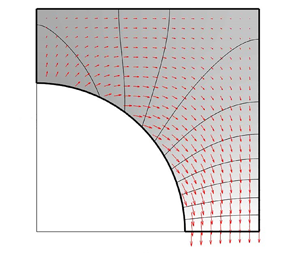
For small wavenumbers, although the cylinder can move only in the $y$-direction, it is the wall distance along $x$ that has the strongest influence. To better understand this paradoxical result, we plot the velocity field in the Fourier space (figure 7). For $k= 10^{-5}$, a strong flow in the $y$-direction (opposite to the cylinder displacement) is observed along the wall $x=l_x$ around the cylinder diameter ($y\approx 0$), as shown in figure 7(a). For large wavenumbers, however, no such flow is observed (figure 7b). By virtue of mass conservation, when the wall distance along $x$ is reduced, this flow increases. This is why there is a strong dependency of the fluid–structure interaction force on the $x$-direction confinements for small wavenumbers.

Figure 7. Velocity and pressure fields in Fourier space for both small and large wavenumbers.

Finally, for all the wavenumbers that have been considered and for all enclosure sizes, the added mass $\hat {\mu }$ appears to increase as the enclosure lengths decrease (in both directions). This observation is in agreement with the literature on channel flows by Chen & Wambsganss (Reference Chen and Wambsganss1972), Chen (Reference Chen1985) and Païdoussis & Pettigrew (Reference Païdoussis and Pettigrew1979).

The calculations performed for a single-cylinder geometry allowed us to prove the reliability of the proposed simplified model. The introduction of the potential flow theory and the use of Fourier transforms are key to relate directly the cylinder displacement and the resulting pressure force.

This approach leads to fast calculations for any kind of geometry. In the next section, it will be applied to a group of cylinders and compared to experimental results in the same geometry.

4.1. ICARE experimental apparatus

The ICARE experimental facility is made of a closed water loop powered by a centrifugal pump, the test section, a compensation tank and a heat exchanger (figure 8). The test section is placed in vertical position with a square section measuring $22.5\ {\rm cm}\times 22.5\ {\rm cm}$, and hosts up to four fuel assemblies arranged in a $2 \times 2$ lattice. The length of the fuel assemblies is $L=2.57$ m. Each of them constitutes a square lattice of $8\times 8$ rods, in which there are 60 rods simulating fuel rods made of acrylic, and four stainless steel guide tubes. The guide tubes are empty inside, and they are welded to five metallic spacer grids along the length of the assembly. The guide tubes have a structural function since they give rigidity to the assembly and they hold together fuel rods. Each assembly has a section measuring $10.1 \times 10.1\ {\rm cm}^{2}$, and the 60 rods constituting it have diameter $2A=9$ mm with pin pitch $P/(2A) = 1.39$. The top and bottom of the assembly are fixed rigidly to the guide tubes, and they are fixed to the test section through the lower and upper support plates.

Figure 8. Scheme of the ICARE experimental facility. LDV, laser Doppler velocimetry.

A hydraulic actuator applies dynamic forcing to one of the four fuel assemblies (assembly [1] in figure 8). This forcing in one dimension aims to simulate an earthquake. The actuator is screwed into one of the grids of the assembly, and a force sensor is installed in between the actuator and the stem.

The test section is equipped with 24 linear variable differential transformer (LVDT) position sensors to measure the displacement of each grid in two directions (figure 9). For more details on the ICARE experiment, please refer to Capanna et al. (Reference Capanna, Ricciardi, Eloy and Sarrouy2019).

Figure 9. Scheme of the displacement sensors on the ICARE test section.

4.2. Problem geometry and meshing

The ICARE geometry is implemented in the code to allow for comparison with experiments with large ($C=8$ mm) or small ($C=4$ mm) confinements (figures 10(a) and 10(b), respectively). Confinement size denotes the length of the gap between different assemblies and between the assemblies and the walls. For both confinement sizes, the distance in between the rods of the same assembly remains the same.

Figure 10. Meshes for the two configurations simulating the ICARE set-up. These two geometries differ only by the value of the confinement $C$, as pictured. (a) Four assemblies in large confinement. (b) Four assemblies in small confinement.

Assemblies are numbered as depicted in figure 10(a). As in the experiments, the rods of assembly [1] are forced along the $x$-direction, and they all exhibit the same displacement $w_{x}^{[1]}(z,t)$. Those rods are assumed not to move along the $y$-direction, and the rods in the other assemblies are assumed not to move.

Based on § 3, the Helmholtz problem to solve is

(4.1a)$$\begin{gather} \Delta\hat{p} = k^{2}\hat{p},\quad \text{in the domain}, \end{gather}$$

(4.1b)$$\begin{gather}\left.\frac{\partial\hat{p}}{\partial n}\right|_{\partial\text{C}_w} = 0, \quad \text{on the walls}, \end{gather}$$

(4.1c)$$\begin{gather}\left.\frac{\partial\hat{p}}{\partial n}\right|_{{\partial}C^{[1]}} = {\hat\omega}_{x}^{[1]}(k,t)\cos(\theta), \quad \text{for assembly [1]}, \end{gather}$$

(4.1d)$$\begin{gather}\left.\frac{\partial\hat{p}}{\partial n}\right|_{{\partial}C^{[n]}} = 0, \quad \text{for other assemblies}, \end{gather}$$

where the superscripts $[n]$ refer to the assembly number, ${\partial}C^{[n]}$ denotes the boundaries of rods of assembly $[n]$ (with $\theta$ the local polar angle for each rod), and

(4.2)\begin{equation} {\hat\omega}_{x}^{[1]}=\mathcal{F}[{(\partial_t+\partial_z)^{2} w_{x}^{[1]}}]. \end{equation}

As in § 3, the solution $\hat {p}$ of the Helmholtz problem (4.1) is proportional to ${\hat\omega}_{x}^{[1]}$, and one can define added masses $\hat {\mu }_x^{[n]}$ and $\hat {\mu }_y^{[n]}$ from the forces exerted on each assembly:

(4.3a)$$\begin{gather} \hat{f}_x^{[n]}(k,t) ={-}\int_{{\partial}C^{[n]}}\hat p\cos(\theta)\,{\rm d}\theta ={-}\hat{\mu}_x^{[n]} {\hat\omega}_{x}^{[1]}, \end{gather}$$

(4.3b)$$\begin{gather}\hat{f}_y^{[n]}(k,t) ={-}\int_{{\partial}C^{[n]}}\hat p\sin(\theta)\,{\rm d}\theta ={-}\hat{\mu}_y^{[n]} {\hat\omega}_{x}^{[1]}. \end{gather}$$

In practice, $\hat {\mu }_x^{[n]}$ and $\hat {\mu }_y^{[n]}$ can be calculated by assuming ${\hat\omega}_{x}^{[1]}=1$ and numerically solving the Helmholtz problem (4.1) for $\hat {p}$. The convergence of the calculations depends on the mesh size. We thus conducted a convergence study and found that convergence is ensured when the walls are divided into at least $150$ sections, and the cylinder borders into $50$ sections. The calculations presented here have been performed with $200$ divisions on the external walls and $75$ divisions on the cylinder borders, which corresponds to approximately 500 000 cells in the domain and a computing time of about 60 s.

Figure 11 shows the results of these computations for $k\in [10^{-5}, 10]$. In Appendix B, we detail these results for individual rods. As in the single-cylinder case, the added masses do not change much for extreme values of $k$, i.e. $k\lesssim 10^{-2}$ or $k\gtrsim 1$, except for assembly $[1]$, the forced assembly. For large $k$, the added masses converge to zero.

Figure 11. Added masses $\hat {\mu }_x^{[n]}$ (blue solid line) and $\hat {\mu }_y^{[n]}$ (red dashed line) on each assembly (in Fourier space) for different values of $k$.

4.3. Equations of motion in real space

The functions $\hat {\mu }_x^{[n]}(k)$ and $\hat {\mu }_y^{[n]}(k)$ can be interpolated using piecewise sixth-order polynomials, which can then be used to calculate ${\mu }_x^{[n]}(z)$ and ${\mu }_y^{[n]}(z)$ with an inverse Fourier transform (Appendix C). By analogy with the calculations for a single cylinder done in § 2.4, we can define added mass, added damping and added stiffness matrices for the assemblies too. There are 24 such matrices: 3 kinds (mass $\boldsymbol{\mathsf{M}}$, damping $\boldsymbol{\mathsf{C}}$, stiffness $\boldsymbol{\mathsf{K}}$), 2 axes ($x$ and $y$, subscript $\circ$) and 4 assemblies, noted with the superscript $[n]$. Similarly to (2.32a–c), these matrices are expressed using the added masses ${\mu }_\circ ^{[n]}(z)$:

(4.4a)$$\begin{gather} {(}\boldsymbol{\mathsf{M}}_\circ^{[n]} )_{ij} = \langle \chi_i, \mathcal{F}^{{-}1}[{\hat{\mu}_\circ^{[n]} \hat{\chi}_j}]\rangle = \frac{1}{2 {\rm \pi}}\langle \chi_i, \mu_\circ^{[n]} \star \chi_j\rangle, \end{gather}$$

(4.4b)$$\begin{gather}{(}\boldsymbol{\mathsf{C}}_\circ^{[n]} )_{ij} = \langle \chi_i, \mathcal{F}^{{-}1}[{2{\rm i}k\hat{\mu}_\circ^{[n]} \hat{\chi}_j} ]\rangle = \frac{1}{2 {\rm \pi}}\langle \chi_i, 2\mu_\circ^{[n]} \star \chi'_j\rangle, \end{gather}$$

(4.4c)$$\begin{gather}{(}\boldsymbol{\mathsf{K}}_\circ^{[n]} )_{ij} = \langle \chi_i, \mathcal{F}^{{-}1}[{-k^{2}\hat{\mu}_\circ^{[n]} \hat{\chi}_j} ]\rangle = \frac{1}{2 {\rm \pi}}\langle \chi_i, \mu_\circ^{[n]} \star \chi''_j\rangle, \end{gather}$$

where $\chi _i(z)$ is the $i$th beam eigenmode defined in (2.29).

Because it is forced at mid-height, we can assume that assembly [1] moves mainly in its first beam eigenmode, i.e. $w_x^{[1]}(z,t) = q_x^{[1]}(t)\,\chi _1(z)$. We can assume further that the added mass and added stiffness matrices are diagonal, and that the added damping is negligible (Appendix C). With these hypotheses, the equation of motion for the $x$-component of assembly [1] is

(4.5)\begin{equation} (m_s + m_x^{[1]})\ddot{q}_x^{[1]} + c_v\,\dot{q}_x^{[1]} + (k_s + k_x^{[1]}) q_x^{[1]} = f_e\,{\rm e}^{{\rm i}\omega t}, \end{equation}

where $m_s=64m$ is the dimensionless mass of one assembly per unit length, $k_s = 64 b k_1^{4}$ is its stiffness, $c_v$ accounts for the damping induced by the viscosity effect, $m_x^{[1]}$ and $k_x^{[1]}$ denote the component $(1,1)$ of the added matrices $\boldsymbol{\mathsf{M}}_x^{[1]}$ and $\boldsymbol{\mathsf{K}}_x^{[1]}$, and $f_e\,{\rm e}^{{\rm i}\omega t}$ is the external forcing projected onto the first eigenmode, with $f_e$ a scalar. The $m_x^{[1]}$ and $k_x^{[1]}$ coefficients represent the added mass and stiffness encountered by an assembly that moves in its first mode in either the $x$-direction or the $y$-direction. Here, we consider only a weak coupling between the assemblies, such that we can neglect the hydrodynamic forces due to the motion of the other assemblies on assembly $[1]$ (the validity of this assumption will be assessed below). The solution of (4.5) is simply

(4.6)\begin{equation} q_x^{[1]} = h_x^{[1]} f_e\,{\rm e}^{{\rm i}\omega t}, \end{equation}

with the transfer function

(4.7)\begin{equation} h_x^{[1]}(\omega) =\frac{1} {-\omega^{2} (m_s + m_x^{[1]}) + {\rm i}\omega c_v + k_s + k_x^{[1]}}. \end{equation}

It is possible to estimate the motion of assemblies [2], [3] and [4] by considering the superimposition of the two following cases: still rods undergoing fluid forces induced by assembly [1] on the one hand, and moving rods undergoing fluid forces generated by their own movement while other assemblies stand still:

(4.8) \begin{equation} (m_s + m_x^{[1]})\ddot{q}_\circ^{[n]} + c_v\,\dot{q}_\circ^{[n]} + (k_s + k_x^{[1]}) q_\circ^{[n]} ={-}(-\omega^{2} m_\circ^{[n]} + k_\circ^{[n]}) q_x^{[1]}, \end{equation}

where the coefficients $m_x^{[1]}$, $c_v$ and $k_x^{[1]}$ appear on the left-hand side because, by symmetry, they also correspond to the pressure force induced by the motion $q_\circ ^{[n]}$ on the assembly $[n]$ itself. The right-hand side represents the action of assembly [1] motion via the fluid.

From (4.4c), we see that the added stiffness is $k_\circ ^{[n]} = -k_1^{2} m_\circ ^{[n]}$, with $k_1 = {\rm \pi}/l$ (since $\chi _i'' = -k_i^{2} \chi _i$). We will now assume that $\omega \gg k_1$, which is true here because typical values of $\omega$ are around 0.3, and $l \approx 571$. This means that the added stiffness term $k_\circ ^{[n]}$ can be neglected compared to the added mass term $-\omega ^{2} m_\circ ^{[n]}$ in (4.5) and (4.8). The values of the added masses $m_\circ ^{[n]}$ are given in table 1. From this table, we see that the ratio of added masses $m_\circ ^{[n]} / m_x^{[1]}$ is at most 21 % (for $n>1$). This justifies neglecting the hydrodynamic forces due to the motion of the assemblies $[n]$ onto assembly $[1]$, which can be estimated as the square of this ratio and is thus of order 4 % at most.

Table 1. Added mass matrix coefficients for small and large confinements.

Under these hypotheses, we can calculate the displacement ratio at the forcing frequency $\omega$ as

(4.9)\begin{equation} \frac{q_\circ^{[n]}}{q_x^{[1]}} \approx{-}\frac{-\omega^{2} m_\circ^{[n]}}{-\omega^{2} (m_s + m_x^{[1]}) + {\rm i}\omega c_v + k_s}, \end{equation}

which becomes, at the resonant frequency $\omega _{res}$,

(4.10)\begin{equation} \frac{q_\circ^{[n]}}{q_x^{[1]}} \approx{-}{\rm i} \omega_{res}\, \frac{m_\circ^{[n]}}{c_v}, \quad \mbox{with } {-\omega}_{res}^{2} (m_s + m_x^{[1]}) + k_s = 0. \end{equation}

Note that this equation is applicable only to $n\neq$1.

4.4. Comparison with a periodic assembly of cylinders

The model presented above allows us to compute the added mass of an assembly of cylinders organised in a square array. A qualitative comparison can be made with an infinite assembly made of a periodic arrangement of cylinders (Pettigrew & Taylor Reference Pettigrew and Taylor2003). In this case, by analogy with (3.4), the added mass of each cylinder is expressed as

(4.11)\begin{equation} \hat{\mu}={\rm \pi}\,\frac{a_{equiv}^{2}+1}{a_{equiv}^{2}-1}, \end{equation}

where $a_{equiv}$ is a measure of the equivalent confinement that can be approximated as

(4.12)\begin{equation} a_{equiv}=\left(0.535+0.14 p\right) p, \end{equation}

with $p=P/A$, the period along $x$ and $y$ of the arrangement.

Using the value $P/A=2.78$ of the ICARE assemblies, (4.11) corresponds to an added mass per cylinder $\hat {\mu }=4.26$. Considering an assembly made of 64 cylinders, the total added mass is $m_x=274$. This value can be compared to the value $m_x^{[1]}=350$ obtained in our simulations (table 1). The two values are of the same order, but in the ICARE geometry, the presence of other assemblies and of the walls tends to increase the added mass.

5.1. Added mass

Let us consider the transfer function $H^{[1]}_{exp}$ between the displacement $W^{[1]}_{x}$ along $x$ of the grid with vertical position $Z_w$, and the force $F_{g}$ applied by the actuator on the grid with position $Z_f$. Since the data are acquired with a swept sinusoidal excitation, the transfer functions are calculated using the cross-correlation product, and are defined as

(5.1)\begin{equation} H^{[1]}_{exp}=\left\|\frac{W^{[1]}_{x} \star W^{[1]}_{x}}{W^{[1]}_{x} \star F_{x}}\right\|, \end{equation}

where $W^{[1]}_{x} \star W^{1]}_{x}$ is the spectral autocorrelation of the displacement signal of the first assembly along the $x$-direction, and $W^{[1]}_{x} \star F_{x}$ is the spectral cross-correlation between the displacement signal of the first assembly and the force imposed on the first assembly. Cross-correlation functions are calculated using an Hamming windowing filter (5000 points per windows) to clean up the noise from the signal.

The theoretical transfer function modulus for a one-degree-of-freedom system is given by

(5.2)\begin{equation} H^{[1]}_{theo}(\varOmega)=\frac{1}{\sqrt{(K_e-\varOmega^{2}M_e)^{2}+\varOmega^{2}C_e^{2}}}, \end{equation}

where $M_e$, $C_e$ and $K_e$ are the coefficients of mass, damping and stiffness identified, and $\varOmega$ is the circular frequency.

Assembly [1] is excited around its first mode; to identify its dynamical properties, one has to find $M_e$, $C_e$ and $K_e$ that make $H^{[1]}_{theo}$ fit the experimental data $H^{[1]}_{exp}$. This can be achieved easily by a conjugate gradient optimisation method.

Using an Euler–Bernoulli beam model for the rods as described in (2.1), one can write the virtual work of assembly [1] as

(5.3)\begin{align} &M_t\int^{L}_{0}\partial^{2}_T W^{[1]}_{x}\,\delta W\,{\rm d}Z+C_t\int^{L}_{0}\partial_T W^{[1]}_{x}\,\delta W\,{\rm d}Z+ B_t\int^{L}_{0}\partial^{2}_Z W^{[1]}_{x}\,\partial^{2}_Z\delta W\,{\rm d}Z\nonumber\\ &\quad=\int_0^{L}F_{g}\,\delta_{Z_f}\,\delta W\,{\rm d}Z, \end{align}

with

(5.4a,b)\begin{equation} M_t=M_s+M_f, \quad B_t=B+B_f, \end{equation}

where $M_f$ and $B_f$ are respectively the participation of the fluid into mass and stiffness, $C_t$ is a linear damping coefficient, and the sum accounts for the 64 rods inside the assembly.

When the structure vibrates on its $j{\rm th}$ natural mode,

(5.5)\begin{equation} W^{[1]}_{x}(Z,T)=N_j(T)\,X_j(Z), \end{equation}

with $X_j(Z)={\chi}j (Z/A)$, one can rewrite the energy of the system as

(5.6)\begin{equation} M_t\int^{L}_{0}X_j^{2}\,{\rm d}Z\,\partial^{2}_T N_j+C_t\int^{L}_{0}X_j^{2}\,{\rm d}Z\,\partial_T N_j+B_t\int^{L}_{0}(\partial^{2}_Z X_j)^{2}\,{\rm d}Z\,N_j=F_{g}\,X_j(Z_f).\end{equation}

Noting that the experimental signal is

(5.7)\begin{equation} W^{[1]}_{g}=N_1(T)\,X_1(Z_w), \end{equation}

one can relate the mass per unit of length to the identified coefficient

(5.8)\begin{equation} M_t=\frac{X_1(Z_f)\,X_1(Z_w)}{\displaystyle\int^{L}_{0}X_1^{2}\,{\rm d}Z}\,M_e. \end{equation}

Measurements take into account the effect of the fluid added mass $M_f$ and the mass of the structure $M_s$, therefore to isolate the fluid added mass, the participation of the structure is subtracted, based on experimental results obtained in air. Finally, one then obtains the results listed in table 2 where added mass values are provided for the whole assembly,

(5.9)\begin{equation} M^{[1]}_x = M_f. \end{equation}

To get a comparison with results from numerical simulation obtained in § 4, the following transformation is applied

(5.10)\begin{equation} M^{[1]}_x = \rho A^{2} \, m_x^{[1]}, \end{equation}

where $\rho =1000\ {\rm kg}\ {\rm m}^{-3}$ is the water density.

Table 2. Values of added mass $M^{[1]}_x$.

Table 2 shows the values of added mass for large and narrow confinement given by experiments and simulations. Both agree on the increase of added mass when the confinement gets narrower. Experiments give a large increase, more than double, whereas simulations predict an increase of about 10 %. Although the order of magnitude is respected, the differences observed could cast doubt on the validity of the model. To analyse these results properly, one has to keep in mind that the methodology used to obtain the experimental results is subject to uncertainties coming from the accuracy of measurement, the optimisation process, and the fact that we try to identify constants of a linear one-degree-of-freedom system from a complex nonlinear system. As a result, one could estimate that the added mass coefficient given by the simulations is a reasonable estimation.

The added stiffness is orders of magnitude smaller than the ‘in air’ structural stiffness: the added stiffness estimated from simulations in § 4 is about $4.7\ {\rm N}\ {\rm m}^{2}$, while the measured flexural stiffness of a fuel assembly is about $2300\ {\rm N}\ {\rm m}^{2}$. As a consequence, we cannot extract the added stiffness from the total stiffness measured experimentally.

5.2. Coupling

To characterise the coupling between the fuel assemblies induced by the fluid, let us consider the transfer function between the imposed displacement and the displacement of the other fuel assemblies at the third grid level in the two transverse directions. Similarly to (5.1), transfer functions are calculated as

(5.11)\begin{equation} H^{[n]}_{{\circ}}=\left\|\frac{W^{[n]}_{{\circ}} \star W^{[n]}_{{\circ}}}{W^{[n]}_{{\circ}} \star W^{[1]}_{x}}\right\|,\quad \circ{\in}\{x,y\}, \end{equation}

where $W^{[n]}$ is the displacement signal of the $n$th assembly along the $\circ$ direction.

For each transfer function, the maximum value – which occurs at the first natural frequency – is accounted for. These experimental results are compared to the displacement ratio given by (4.10), with the added mass coefficients $m_\circ ^{[n]}$ given in table 1, and $c_v$ and $\omega _{res}$ estimated from identification of dynamical parameters using (5.6) as follows:

(5.12a–c)\begin{equation} C_v=\frac{X_1(Z_f)\,X_1(Z_w)}{\displaystyle\int^{L}_{0}X_1^{2}\,{\rm d}Z}\,C_e, \quad c_v=\frac{C_v}{\rho UA}, \quad \omega_{res}=\frac{A}{U}\sqrt{\frac{K_e}{M_e}}. \end{equation}

Experimental values give $c_v=69.2$ and $\omega _{res}=0.12$.

Figure 12 compares graphically the displacement ratios as observed in the experiments with the ratios predicted by (4.10) with these values of $c_v$ and $\omega _{res}$. Experiments show a ratio of about 10 % for most of the fuel assemblies in the two directions except for fuel assembly [3], which shows a coupling of about 20 % in the direction of forcing. Although simulations seem to underestimate the values of coupling, they give a good prediction of the order of magnitude. Moreover, the general pattern is well reproduced, with a significantly more important coupling for fuel assembly [3] in the direction of forcing. Therefore, the methodology developed seems to be appropriate to simulate the coupling between fuel assemblies.

Figure 12. Displacement ratios obtained by experimental data (a) and approximated from numerical simulations (b) for four fuel assemblies in large confinement at first natural frequency.