3.1. Secondary flow structures

Before presenting the effect of the surface heterogeneity on global flow parameters, we examine the spatial development of the secondary flows in the low-Reynolds-number cases with $(\lambda _x, \lambda _y) = (8{\rm \pi}, {\rm \pi}/4)$ and $(\lambda _x, \lambda _y) = (8{\rm \pi}, {\rm \pi}/2)$ to get an idea of what the flow structure in general looks like. As usual in studies concerning secondary flow, we use the mean-signed swirling strength, $\bar {\varLambda }_{ci} = \bar {\lambda }_{ci} \bar {\omega }_x/|\bar {\omega }_x|$, to visualize the streamwise roll motions. Here, $\bar {\lambda }_{ci}$ is calculated as the imaginary part of the complex eigenvalue of the local (time-averaged) velocity gradient tensor on the $yz$-plane (Zhou et al. Reference Zhou, Adrian, Balachandar and Kendall1999; Anderson et al. Reference Anderson, Barros, Christensen and Awasthi2015). The sign of the vorticity is used to indicate direction of the rotation. Signed swirling strength is generally recognized to be a more satisfactory way of identifying swirling motions than the vorticity itself, as the latter cannot distinguish between genuine vortex motions and regions of strong shear (Castro et al. Reference Castro, Kim, Stroh and Lim2021).

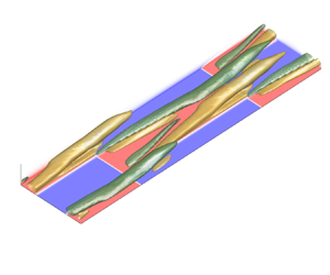
Isocontours of time- and phase-averaged mean signed swirling strength of layout X8Y0.25 are depicted in figure 2(a), with contour levels at 10 % of the maximum and minimum values. Note that the original domain is 16 times larger in the $y-$direction, but phase-averaging was applied. We observe two longitudinal roll structures that emerge from the streamwise transition at $x/h=2{\rm \pi}$. The streamwise development of the secondary motions can be appreciated more clearly in the $yz$-planes in figure 2(c,e,g), depicting contour plots of signed swirling strength with vectors of spanwise and vertical velocity. The streamwise locations where the planes are taken, $x/h \in \{2.5{\rm \pi}, 4{\rm \pi}, 5.5{\rm \pi} \}$, are also illustrated in figure 2(a). Figure 2(c) clarifies that the two vortices are formed right above the spanwise temperature step, and their extent grows as the flow travels downstream. In the last two planes (figure 2e,g), the size and strength of the swirling motions is nearly equal, indicating that the secondary flow could be considered to be fully developed. Behind the streamwise transition at $x/h=6{\rm \pi}$, the roll structures move upward and eventually fade out. This is also visible in figure 2(c), where the two upper vortices are a remainder of the secondary flows that have developed over the upstream section ($x/h < 2{\rm \pi}$).

Figure 2. (a,c,e,g) Layout X8Y0.25, (b,d, f,h) layout X8Y0.5. (a,b) Time- and phase-averaged isosurfaces of signed swirling strength $\bar {\varLambda }_{ci}$. Contour levels are 10 % of the maximum and minimum values, while colours indicate positive (yellow) and negative (green) values. Bottom and side planes indicate potential temperature reduced with its horizontal average ($\bar {\theta }''=\bar {\theta } - \langle \bar {\theta }\rangle$). (c–h) Time- and phase-averaged $yz$-planes of signed swirling strength, at $x=2.5{\rm \pi}, 4{\rm \pi}$ and $5.5{\rm \pi}$, as also indicated in (a,b). Vectors are constructed from mean spanwise and vertical velocity. Red and blue lines at the bottom correspond to high and low surface temperature. Note that the spanwise axes are reversed to have them aligned with the 3-D plots in (a,b). The aspect ratio in all plots is 4:1:1.

Figure 2(b,d, f,h) present the same variables, but for layout X8Y0.5. Compared with layout X8Y0.25, only the width of the hot and cold patches is doubled. In this scenario as well, two counterrotating vortices arise just above the spanwise temperature transitions, and they develop downstream to become the main secondary flow. Above the centre of the hot patch however, a weaker vortex pair forms, rotating in opposite direction to the adjacent main secondary motions (see figure 2d, f). Such tertiary flows have also been reported in flows over spanwise varying surface stress (Stroh et al. Reference Stroh, Hasegawa, Kriegseis and Frohnapfel2016) and longitudinal ridges (Hwang & Lee Reference Hwang and Lee2018; Castro et al. Reference Castro, Kim, Stroh and Lim2021). We remark that in the present case, this may be more counter-intuitive as we observe downward motion above a high-temperature patch, where the buoyancy force is upward. As the flow travels downstream, the extent of the strongest vortices grows until the tertiary vortices have disappeared near the end of the patch (figure 2h) and the two main vortices dominate the flow.

Comparing the left and right columns in figure 2 reveals that the main difference between the two cases with layouts X8Y0.25 and X8Y0.5 are the tertiary flows that develop above the wider patch. In addition to that, the magnitude of the swirling strength and the vectors are larger for the case with $\lambda _y/h = {\rm \pi}/2$. Finally, the secondary motions in the case with $\lambda _y/h={\rm \pi} /4$ seem to reach a fully developed state, where there only are minimal changes in the streamwise direction from approximately $2{\rm \pi} h$ downstream of the transition. In contrast, the last two contours in the case with $\lambda _y/h={\rm \pi} /2$ (figure 2 f,h) are less similar, illustrating that the secondary motions are still changing in the streamwise direction.

To investigate the strength and streamwise development of the secondary motions in a more quantitative way for all simulations, we consider two measures that are commonly used to describe the intensity of the secondary circulations. The first is based on the magnitude of the cross-stream velocity components $\psi = (\bar {v}^2 + \bar {w}^2)^{1/2}$, whereas the second involves the streamwise vorticity $\omega _x = \partial \bar {w}/\partial y - \partial \bar {v}/\partial z$. Both are calculated from the time- and phase-averaged $v$ and $w$ fields. The three-dimensional $\psi$ and $\omega _x$ arrays are then consecutively squared and averaged over the spanwise and vertical directions, defining

(3.1a,b)\begin{equation} \varOmega_x(x) = \frac{1}{A}\int_0^{2h} \int_0^{\lambda_y} \omega_x^2 \,\text{d}y\,\text{d}z \quad \text{and} \quad \varPsi(x) = \frac{1}{A}\int_0^{2h} \int_0^{\lambda_y} 0.5\psi^2 \,\text{d}y\,\text{d}z, \end{equation}

where $A = 2h\lambda _y$ is the area of the cross-stream plane. The former is the specific mean streamwise enstrophy, which can be interpreted as a measure of the rotational energy contained in the secondary motions (Stroh et al. Reference Stroh, Schäfer, Frohnapfel and Forooghi2020b). Likewise, the latter is related to the volume-averaged kinetic energy contained in the cross-stream velocity (Schäfer et al. Reference Schäfer, Frohnapfel and Mellado2022; Zampino et al. Reference Zampino, Lasagna and Ganapathisubramani2022). To enable comparison of the secondary motions in the 2-D heterogeneous cases to the equivalent streamwise homogeneous cases, we normalize $\varOmega _x$ and $\varPsi$ first by the bulk velocity $u_b = (1/2h) \int _{0}^{2h} \langle \bar {u} \rangle {\textrm d}z$ and finally by the average value from the corresponding streamwise homogeneous simulation, denoted by subscript Xh.

The ratios of normalized mean cross-stream velocity and enstrophy that are then obtained are displayed in figure 3. To generalize the length along the streamwise direction, we subtract the location of the streamwise transition ($x_t$) and normalize by the spanwise width of the temperature patches, i.e. $(x-x_t)/l_y$. Since the development over only one patch length is shown ($0 < x-x_t < l_x=\lambda _x/2$), the total length of the lines in figure 3 corresponds to the aspect ratio $a = l_x/l_y = \lambda _x/\lambda _y$ of the rectangular temperature patches. With this normalization, we observe some similarity for cases with the same aspect ratio, if $a \ge 8$. In particular, the two cases with the largest aspect ratio (darkest red and blue lines) converge to a value of $[\varOmega _x(x)/u_b^2]/[\langle \varOmega _x\rangle /u_b^2]_{Xh} \approx [\varPsi (x)/u_b^2]/[\langle \varPsi \rangle /u_b^2]_{Xh} \approx 1$ for $x-x_t \gtrsim 25 l_y$, suggesting that the secondary motions need approximately 25 times the spanwise width to reach the same strength as they would have if the patches were infinitely long. Directly downstream of the streamwise transition, the total strength of the secondary motions decreases as the ‘new’ secondary motions are forming and the secondary motions formed above the downstream patch are diminishing. Remarkably, the locations of the local minimum in $\varPsi$ (at $x-x_t \approx 4l_y$) and $\varOmega _x$ (at $x-x_t \approx 2l_y$) are very similar for all cases with $Re_\tau =180$ and $a \ge 8$. Downstream of this minimum, the secondary motion strength increases further and the enstrophy even exceeds the streamwise homogeneous value with a peak around $x-x_t \approx 10l_y$. We hypothesize that this large enstrophy may be due to strong shear near the surface, where $\partial v/\partial z \gg \partial w/\partial y$, rather than that the secondary motions are actually stronger. In the cross-stream velocity ratio, this local maximum at $x-x_t = 10l_y$ does not exceed unity.

Figure 3. Ratio of (a) integrated cross-stream velocity $\varPsi$ and (b) vorticity $\varOmega _x$ with respect to the equivalent streamwise homogeneous case. The $x$-axis starts at the location of a streamwise transition $x_t$ and is scaled with patch width $l_y$. Only one patch is shown, such that the length of the lines corresponds to the patch aspect ratio $a$. Blue lines indicate surface layouts with $\lambda _y/h = {\rm \pi}/4$, red lines $\lambda _y/h = {\rm \pi}/2$ and dashed lines represent cases with $Re_\tau =550$. Darker lines illustrate longer patches (larger $\lambda _x/h$).

The findings in figure 3 suggest that for relatively long strips ($a \ge 8$), the streamwise development of the secondary motions is governed by the patch aspect ratio rather than the patch length. An intuitive explanation would be that the initial spanwise separation between the secondary motions, as they start to develop close to the surface, is larger if $\lambda _y/h$ is larger (cf. figure 2c,d). Consequently, the two main counterrotating vortices require more distance to reach each other above the centre of the patch, where they eventually reinforce each other. Furthermore, as discussed in the previous section, the tertiary vortices arising between the two ‘main’ circulations for the cases with wider patches may prevent them from merging faster. However, we emphasize that a wider range of patch widths should be considered to draw a more general conclusion.

The cases with $Re_\tau = 550$, indicated by dashed lines in figure 3, show qualitatively similar behaviour to the cases with lower Reynolds number. In the simulation with layout X8Y0.5, the streamwise enstrophy reaches the same magnitude as the streamwise homogeneous case, while the maximum $\varPsi$ is approximately 80 %. The location of the minimum $\varPsi$ and $\varOmega _x$ is shifted further downstream compared with the cases with $Re_\tau = 180$. Both observations imply that at higher Reynolds number, the secondary flows diminish and grow over a larger distance but at a smaller rate.

Lastly, it is clear that the secondary flows are much less significant in the channels with shorter patches ($a \lesssim 4$ or $\lambda _x/h \lesssim {\rm \pi}$), since the averaged cross-stream velocity and enstrophy are smaller than ${\sim }10$% of the streamwise homogeneous value.

3.2. Global flow properties

In this subsection, we will analyse the effect of heterogeneous surface temperature and the induced secondary motions on domain-averaged flow characteristics, which are also reported in table 1. The bulk Reynolds and Richardson numbers there are defined as $Re_b = u_b h/\nu$ and $Ri_b = gh\beta \Delta _z\theta /(2 u_b^2)$, allowing comparison to studies with fixed flow rate $u_b$. In addition, the stability parameter $h/L_{O}$, which is often used in the ABL community to characterize stability of the surface layer, is also presented. The Obukhov length given by

(3.2)\begin{equation} L_O = \frac{u_\tau^3}{\kappa g\beta \alpha \left(\dfrac{\partial \langle \bar{\theta}\rangle}{\partial z} \right)_w} \end{equation}

can be interpreted as the height at which the buoyancy flux is of the same order as the turbulent energy production (Nieuwstadt Reference Nieuwstadt2005; Flores & Riley Reference Flores and Riley2011). In the definition above, $\kappa \approx 0.4$ is the Von Kármán constant and $(\partial \langle \bar {\theta }\rangle /\partial z)_w$ is the temperature gradient averaged over the bottom and top wall. The Obukhov length also plays a central role as a scaling parameter in MOST, which will be discussed in § 3.4. According to Nieuwstadt (Reference Nieuwstadt2005), flows with $h/L_O \gtrsim 0.51$ exhibit intermittent or fully collapsed turbulence and therefore belong to the strongly stably stratified regime (van Hooijdonk et al. Reference van Hooijdonk, Moene, Scheffer, Clercx and van de Wiel2017). Later studies suggest the Obukhov–Reynolds number as a parameter that governs the transition from weak to strong stratification, with $Re_L = Re_\tau L_O/h \approx 200$ as a critical value (Flores & Riley Reference Flores and Riley2011; Deusebio et al. Reference Deusebio, Brethouwer, Schlatter and Lindborg2014; Zhou, Taylor & Caulfield Reference Zhou, Taylor and Caulfield2017). In both classifications, all of the present cases fall well within the weakly stable regime (see table 1), implying that turbulence is continuous in our simulations and we do not need to consider effects of intermittency.

The skin friction coefficient and Nusselt number, defined as

(3.3a,b)\begin{equation} C_f=2\frac{u_\tau^2}{u_b^2}, \quad \textit{Nu} = \frac{2h}{\Delta_z \theta} \left(\frac{\partial \langle \bar{\theta}\rangle}{\partial z} \right)_w, \end{equation}

are commonly used to quantify momentum and heat transfer in stably stratified channel flows (García-Villalba & del Álamo Reference García-Villalba and del Álamo2011; Zonta & Soldati Reference Zonta and Soldati2018; Bon & Meyers Reference Bon and Meyers2022), and will now be considered to investigate the effect of the varying surface temperature configuration in our simulations. It may be useful here to realize that the stability parameter $h/L_O$ and Nu are directly related by external parameters since $h/L_O = (\kappa /2) Ri_\tau \textit {Nu} (Pr Re_\tau )^{-1}$. Figure 4(a,b) presents $C_f$ and Nu, normalized by the value from the fully homogeneous simulation, as a function of the (inverse) aspect ratio of the temperature patches. Focusing on the cases with $Re_\tau =180$ (full lines), it is clear from figure 4(a) that friction is significantly increased for infinitely long patches ($k_x/k_y=0$), as reported by Bon & Meyers (Reference Bon and Meyers2022). When the patch aspect ratio and thus the patch length is reduced (i.e. $k_x/k_y$ is increased), the skin friction coefficient drops substantially. For $a=2$, $C_f$ is within 5 % of the homogeneous value. In the higher-Reynolds-number cases (dashed lines), the impact of the heterogeneous surface on the friction coefficient is much smaller and $C_f/C_{f,{hom}}$ drops below 1. This small drag reduction due to the thermal heterogeneous surface was already reported by Bon & Meyers (Reference Bon and Meyers2022) for the $k_x=0$ case, where it was attributed to a decrease in turbulent shear stress. Here, we find that the drag reduction is slightly enhanced for finite-length strips, i.e. the X8Y0.5 layout shows a 5 % decrease with respect to the homogeneous case. Although a deeper analysis of the physical mechanism behind the observed drag reduction is beyond the scope of the present work, we note that Hickey et al. (Reference Hickey, Younes, Yao, Fan and Mouallem2020) demonstrated as well that localized heating by streamwise-aligned heating strips can lead to modest drag reduction in an unstratified, low-Mach-number channel flow with similar $Re_\tau$.

Figure 4. (a) Skin friction coefficient $C_f$ and (b) Nusselt number Nu as a function of surface wavenumber ratio $k_x/k_y$, normalized by the value from the corresponding homogeneous simulations. (c) Dispersive contributions to skin friction coefficient and (d) Nusselt number, relative to the total value.

In figure 4(b), we observe that heat transfer is reduced in channels with infinitely long spanwise heterogeneity and, for the longest finite-length patches, this reduction is just larger. As the temperature patches become shorter ($k_x/k_y$ increases), the Nusselt number increases and at $a= 2$, it is within 2 % of the homogeneous value. A very similar trend is followed by the cases with higher Reynolds number.

To assess the effect of the secondary motions on these patterns, we follow Bon & Meyers (Reference Bon and Meyers2022), by applying a triple decomposition to split $C_f$ and Nu into a laminar, turbulent and dispersive contribution. Triple decomposition is widely used to assess flows with spatial heterogeneities (e.g. Raupach & Shaw Reference Raupach and Shaw1982; Nikora et al. Reference Nikora, McEwan, McLean, Coleman, Pokrajac and Walters2007; Li & Bou-Zeid Reference Li and Bou-Zeid2019), and is obtained from averaging a variable in space and time. Hence, we split a variable into three components:

(3.4)\begin{equation} \phi(x,y,z,t) = \langle \bar{\phi} \rangle(z) + \bar{\phi}''(x,y,z) + \phi'(x,y,z,t), \end{equation}

where it is important to emphasize that $\bar {\phi }''(x,y,z) = \bar {\phi }(x,y,z) - \langle \bar {\phi } \rangle (z)$ represents the time-averaged local deviation from the mean profile and is typically referred to as the dispersive or coherent fluctuation. Further, $\langle \bar {\phi } \rangle$ is the horizontal and time average, while $\phi '$ represents the random or turbulent fluctuation. When this time–space averaging procedure is applied to the convective terms of the governing equations, dispersive fluxes $\langle \bar {u}_i'' \bar {u}_j''\rangle (z)$ and $\langle \bar {w}'' \bar {\theta }''\rangle (z)$ arise (see (B1) and (B2)). Physically, these terms result from the transport by the mean (time-averaged) coherent flow structures (Li & Bou-Zeid Reference Li and Bou-Zeid2019), such as the persistent mean secondary circulations induced by spanwise surface heterogeneity.

By means of vertical integration and a specific normalization, the contribution of the dispersive fluxes to the friction coefficient is then given by

(3.5)\begin{equation} C_f^D ={-} \frac{6}{u_b^2h} \int_{0}^{h}\left(1 - \frac{z}{h} \right) \langle \bar{u}''\bar{w}'' \rangle {\textrm d}z. \end{equation}

We refer to Stroh et al. (Reference Stroh, Schäfer, Forooghi and Frohnapfel2020a) for a derivation of the full decomposition of $C_f$ in a laminar, turbulent and dispersive part, which is also applied by Bon & Meyers (Reference Bon and Meyers2022). Similarly, the dispersive contribution to the Nusselt number is (Fukagata, Iwamoto & Kasagi Reference Fukagata, Iwamoto and Kasagi2005; Bon & Meyers Reference Bon and Meyers2022)

(3.6)\begin{equation} \textit{Nu}^D ={-} \frac{2}{\alpha \Delta^z\theta} \int_{0}^{h} \langle \bar{w}''\bar{\theta}''\rangle {\textrm d}z. \end{equation}

The ratio of the dispersive contribution to the total $C_f$ and Nu are displayed in figure 4(c,d). This shows that the dispersive momentum transfer contributes 20 to 35 % to the total friction for very long strips, and decreases to 5 % or less for $a \le 8$ (or $k_x/k_y \ge 0.125$). The dispersive component of the Nusselt number shows a rather similar trend, except that its sign is negative, which will be discussed further in the next section (see also Bon & Meyers Reference Bon and Meyers2022). At higher Reynolds number (dashed lines), the contribution of the dispersive fluxes is smaller and drops faster as $a$ increases. In general, we can conclude that the effect of the heterogeneity-induced mean secondary flows on the vertical momentum and heat transfer is significant, but it is strongly reduced as the patch aspect ratio reduces. To allow direct comparison of the strength of the thermally induced streamwise secondary motions in the present study to the cases with roughness-induced secondary flows of Schäfer et al. (Reference Schäfer, Frohnapfel and Mellado2022), the volume-averaged coherent (or dispersive) kinetic energy of the cross-sectional velocity components, $K''_c = 0.5\langle \bar {v}''\bar {v}'' + \bar {w}''\bar {w}'' \rangle _{xyz}$, is reported in the last column of table 1. Since the cross-sectional global mean velocity components $\langle \bar {v} \rangle$ and $\langle \bar {w}\rangle$ are zero, this quantity is simply the streamwise average of $\varPsi (x)$ as defined in (3.1a,b) and shown in figure 3. The values of $K_c''/u_\tau ^2$ for the cases with the longest strips are of the order of $10^{-2}$, which agrees very well with the range of 0.01–0.07 in figure 12(a) of Schäfer et al. (Reference Schäfer, Frohnapfel and Mellado2022), indicating that the strength of the thermally induced secondary motions here is similar to the secondary flows that are generated by streamwise-aligned Gaussian ridges under neutral or weakly unstable stratification in their study. We note however that a direct comparison of the two generation mechanisms may not be fair, since the magnitude of the induced secondary motions depends on many different factors. Although the Reynolds number and spanwise heterogeneity length scale are similar in both studies, a comparison of the ‘amplitude’ of the heterogeneity (i.e. the differences in roughness, temperature or heat flux at the surface) would obviously be ambiguous.

3.3. Variance and covariance distributions

The signs of the dispersive contributions to $C_f$ and Nu in the previous section reveal that there is a negative spatial correlation between $\bar {u}''$ and $\bar {w}''$, and a positive spatial correlation between $\bar {w}''$ and $\bar {\theta }''$. To examine this further, we investigate the horizontal distribution of these three components along with the viscous, turbulent and dispersive components of the vertical heat and momentum fluxes (see (B1) and (B2)). Note that mean profiles of these fluxes are presented in Appendix B.1 for completeness.

Figure 5 displays phase- and time-averaged $xy$-planes at $z/h = 0.1$ for layout X8Y0.5, where the black dashed lines indicate the location of the temperature transitions at the underlying bottom surface. At this approximate height, the dispersive fluxes are maximal for this case, as shown in figure 11 of Appendix B.1. The temperature distribution in figure 5(a) shows that the central patch is warmer than average, but the pattern at $z/h = 0.1$ is slightly shifted downstream compared with the surface temperature. In accordance with figure 2, we see two ‘legs’ of upward motions ($\bar {w}'' > 0$) in figure 5(b), which merge further downstream above the centre of the high-temperature patch ($\bar {\theta }'' > 0$). Consequently, the dispersive heat transfer, which is the product of these two terms as displayed in figure 5( f), is mostly positive. Moreover, figure 5(g) shows a negative temperature gradient above the high-temperature patch, implying there is an unstably stratified region in the flow where vertical motions are not damped. This explains the enhanced vertical turbulent and dispersive transport of both heat and momentum in that region in figure 5(e, f,h,i). Moreover, the turbulent heat transfer in this convective region is positive, while it is negative in the stably stratified zones above the low-temperature areas. As such, we find that both the turbulent and dispersive heat transfer above the high-temperature patches are opposite to the mean gradient, but not against the local one.

Figure 5. Horizontal phase- and time-averaged planes at $z/h = 0.1$ for layout X8Y0.5 with $Re_\tau = 180$. Black dashed lines indicate boundaries of underlying temperature patches. (a) Spatial fluctuations of potential temperature, (b) vertical and (c) streamwise velocity. (d,e,f) Laminar, turbulent and dispersive heat flux. (g,h,i) Laminar, turbulent and dispersive momentum flux.

Regarding the streamwise velocity distribution, figure 5(c) reveals that the streamwise velocity is significantly reduced in the convective region above the hot temperature patch, since $\bar {u}''= \bar {u}(x,y) - \langle \bar {u}\rangle < 0$. Here, low-momentum fluid from near the bottom is brought upward by the vertical motions. In the regions where the temperature is below average, downdrafts bring high-momentum fluid from above downward, resulting in an increased streamwise velocity in these regions. These alternating high and low momentum pathways (HMPs and LMPs) are commonly found in studies with secondary motions induced by spanwise heterogeneity (e.g. Barros & Christensen Reference Barros and Christensen2014; Salesky et al. Reference Salesky, Calaf and Anderson2022). The correlation between streamwise and vertical velocity deviations is emphasized in figure 5(i), which shows that the magnitude of the dispersive momentum flux $\langle \bar {u}''\bar {w}''\rangle$ is maximal in the centre between the counter-rotating vortices. Furthermore, figures 5(g) and 5(h) show that the strongest laminar and turbulent momentum fluxes also occur in the unstably stratified areas above the high-temperature patches.

In summary, we conclude from figure 5 that the convective regions above the high-temperature patches play a crucial role in the vertical transport of heat and momentum. In these zones, all heat transfer components are in the opposite direction with respect to the stable regions, explaining the reduction in overall heat transfer (i.e. Nu) due to the temperature heterogeneity that we found in the preceding section. Moreover, the rise in friction coefficient induced by the inhomogeneous surface can be related to the increased magnitude of both turbulent and dispersive momentum transfer in the unstably stratified sections.

Lastly, we study the effect of the thermal heterogeneity on the variances of streamwise velocity and temperature. Analogous to the vertical fluxes, the variances (or normal stresses in the case of velocity components) can also be decomposed into a turbulent and dispersive part, denoted respectively by $\langle \overline {\phi '\phi '}\rangle$ and $\langle \bar {\phi }''\bar {\phi }''\rangle$. The latter provides information on the penetration depth of the heterogeneity, also referred to as the blending height. This is the height above which the flow is homogeneous (Bou-Zeid, Meneveau & Parlange Reference Bou-Zeid, Meneveau and Parlange2004) and therefore the dispersive normal stresses are zero. Figure 6(a) shows mean profiles of the total (turbulent $+$ dispersive) normal stress (full lines) and the dispersive contribution (dashed lines) for the cases with $Re_\tau =180$ and $\lambda _y/h = {\rm \pi}/2$. The significant streamwise dispersive stress reveals that the streamwise velocity is highly heterogeneous, which is strongly associated with the formation of HMPs and LMPs as explained above and shown in figure 5(c). The fact that the dispersive stresses and fluxes are negligible in the channel core confirms that the channel centre is homogeneous in all cases. Interestingly, we observe that the total variance, $\langle \overline {u'u'}\rangle + \langle \bar {u}''\bar {u}''\rangle$ (full lines), remains approximately equal among all cases, suggesting that dispersive and turbulent variance act like communicating vessels. Furthermore, this implies that the turbulent stress is reduced in the cases where the dispersive stress is large (not shown). The reduction of turbulent stresses in the presence of secondary flows was shown previously by Medjnoun, Vanderwel & Ganapathisubramani (Reference Medjnoun, Vanderwel and Ganapathisubramani2020) and Stroh et al. (Reference Stroh, Schäfer, Forooghi and Frohnapfel2020a) in neutral flow conditions, and can possibly be explained by the fact that there is more temporal coherence in the flow due to the spatially fixed surface heterogeneity.

Figure 6. Horizontally averaged profiles of (a) streamwise normal stresses and (b) temperature variances, for cases with $Re_\tau =180$ and $\lambda _y/h = {\rm \pi}/2$. The full lines in (a) represent the total velocity stress (dispersive $+$ turbulent), while in (b), full lines denote only the turbulent fluctuations. Dashed lines show dispersive variances. In (b), the left ordinate belongs to dispersive component (dashes) and the right ordinate to turbulent component (full lines). Inset in (b) shows zoom of dispersive temperature variance, where the arrow indicates the direction of increasing temperature patch length.

The temperature variances in figure 6(b) expose that the dispersive temperature fluctuation (dashed lines, left ordinate) in the near-wall region is nearly two orders of magnitude larger than the turbulent variance (full lines, right ordinate), but decreases sharply away from the wall. In fact, the value of $\langle \bar {\theta }'' \bar {\theta }''\rangle$ at the surface is directly determined by the heterogeneous boundary conditions (figure 1) and is therefore equal for all cases. The inset in figure 6(b) shows that the dispersive temperature variance decays faster for smaller $\lambda _x/h$, implying that horizontal temperature mixing is stronger in the presence of streamwise heterogeneity. This enhanced mixing is accompanied by larger turbulent temperature fluctuations, as evidenced by the observation that the peak in turbulent temperature variance (full lines) close to the wall is higher for most layouts with small $\lambda _x/h$, while there is no near-wall peak in the homogeneous case (black line). The conclusion that heterogeneous temperature boundary conditions enhance temperature variance close to the surface was already made by Mironov & Sullivan (Reference Mironov and Sullivan2016, Reference Mironov and Sullivan2023) in their respective LES and DNS studies with streamwise varying surface temperature, although they did not distinguish between dispersive and turbulent components (see § 3.5). The dispersive variance is negligible for $z/h \gtrsim 0.15$, indicating that the blending height for temperature is significantly lower than that for streamwise momentum.

3.4. Monin–Obukhov similarity and outer layer scaling

The preceding sections demonstrate that surface temperature heterogeneity can have significant impact on the flow, penetrating deeply into the outer layer. In this section, we evaluate two existing methods to scale mean velocity and temperature profiles in the outer layer, and see to what extent they can be applied in these heterogeneous channel flows.

To this end, we first use the local Monin–Obukov similarity theory (MOST), which is widely used to interpret ABL data. Previous DNS studies have shown that homogeneous stable channel flow at sufficiently high Reynolds number agrees reasonably well with (local) Monin–Obukhov scaling (García-Villalba & del Álamo Reference García-Villalba and del Álamo2011; He Reference He2016; He & Basu Reference He and Basu2016). We note that at low Reynolds numbers, the intermediate layer where MOST is valid, between the viscous sublayer and the internal-wave-dominated channel centre, is not present (García-Villalba & del Álamo Reference García-Villalba and del Álamo2011; Shah & Bou-Zeid Reference Shah and Bou-Zeid2014). The original MOST assumes that all fluxes are constant with height, and employs the Obukhov length as defined in (3.2) based on surface momentum and temperature fluxes. In the current stable channel flows, the fluxes are not constant (figures 11 and 12c,d). Therefore, the dynamics in the outer region is governed by a local scaling based on a local Obukhov length (Nieuwstadt Reference Nieuwstadt1984):

(3.7)\begin{equation} \varLambda(z) = \frac{u_*(z)^3}{\kappa g\beta q_z}, \end{equation}

with $u_*(z) = (\tau _{xz})^{1/2}$ as in (B1) and $q_z$ as in (B2). Note that with this definition, the laminar and dispersive fluxes are also explicitly included in the framework, while the original MOST is based on homogeneous flow at infinite Reynolds number and therefore only includes the turbulent fluxes (Shah & Bou-Zeid Reference Shah and Bou-Zeid2014). Nevertheless, recent DNS studies involving heterogeneous surfaces have also incorporated laminar and (implicit) dispersive fluxes in their comparisons to MOST (Lee, Gohari & Sarkar Reference Lee, Gohari and Sarkar2020; Mironov & Sullivan Reference Mironov and Sullivan2023). Figure 7(a) shows profiles of the local Obukhov length scale for the present simulations with $Re_\tau =550$. Given that $u_*(0) = u_\tau$ and $q_z$ is constant through the channel (see Appendix B.2), $\varLambda (0)$ corresponds to the Obukhov length $L_O$ as reported in table 1. The local Obukov length is maximal for layout XhY0.5, and decreases with streamwise wavelength and wall distance. The dashed lines in figure 7(a) indicate $\varLambda (z)$ without inclusion of the dispersive fluxes. These are significantly smaller for the cases with the longest temperature patches, where the secondary flows are most significant.

Figure 7. (a) Local Obukhov length as a function of wall distance. (b) Mapping of stability parameter $z/\varLambda$ onto wall distance $z/h$. Similarity functions for (c) momentum and (d) heat. Coloured dashed lines indicate calculations without dispersive fluxes. Grey dashed lines in (a,b) represent limits for $z/h$ that have been used for data in (c,d). Light dashed lines in (c,d) depict empirical linear relation $1+4.7z/\varLambda$.

Within the MOST framework, the similarity functions for the non-dimensional shear $\varPhi _m$ and temperature gradient $\varPhi _h$ are

(3.8a)$$\begin{gather} \varPhi_m\left(\frac{z}{\varLambda}\right) = \frac{\kappa z}{u_*(z)}\frac{\partial \langle \bar{u}\rangle}{\partial z} \approx 1+\beta_m \frac{z}{\varLambda(z)}, \end{gather}$$

(3.8b)$$\begin{gather}\varPhi_h\left(\frac{z}{\varLambda}\right) = \frac{\kappa z}{\theta_*(z)}\frac{\partial \langle \bar{\theta}\rangle}{\partial z} \approx \alpha_h+\beta_h \frac{z}{\varLambda(z)}, \end{gather}$$

where the local friction temperature $\theta _*(z) = q_z/u_*(z)$. Although MOST does not specifically predict the shape of these functions, it has been established empirically that under stable conditions, both are linear in $z/\varLambda$ as indicated by the right-hand side of (3.8). While the exact values of the linear coefficients differ across different publications, we use typical values of $\alpha _h = 1$ and $\beta _m = \beta _h = 4.7$ (Stull Reference Stull1988; Hogstrom Reference Hogstrom1996; He Reference He2016).

Figures 7(c) and 7(d) depict the stability functions $\varPhi _m$ and $\varPhi _h$ for all cases at $Re_\tau = 550$. To avoid the impact of molecular viscosity at the bottom and internal waves in the channel centre, we only consider data from $0.01 < z/h < 0.8$ ($5 < z^+ < 440$), as indicated by the grey dashed lines in figure 7(a,b).

First, we find that the profiles from the homogeneous channel (black lines) agree reasonably well with the proposed linear relation for $z/\varLambda \gtrsim 0.05$, justifying the comparison of our DNS data at moderate Reynolds number to MOST. Note that we can use the mapping provided in figure 7(b) to determine that $z/\varLambda = 0.05$ corresponds to $z/h \approx 0.1$. The scaled velocity gradient profiles of all heterogeneous cases with finite length show excellent collapse; however, this outcome may be rather unsurprising since the velocity profiles are already highly similar before any scaling is applied (see Appendix B.2, figure 12a). The collapse of $\varPhi _h$ profiles on the other hand depends clearly on the surface layout, while for $z/\varLambda \gtrsim 0.35$ ($z/h \gtrsim 0.45$), all layouts with finite-length temperature patches are similar. For layout XhY0.5, where the temperature strips are infinitely long, the velocity and temperature gradient profiles in the outer layer have a comparable slope but are shifted downwards.

To assess the influence of dispersive fluxes in the present MOST framework, we also calculated the scaling functions and local Obukhov length without taking the dispersive fluxes into account. Resulting profiles are depicted by the dashed lines in figure 7. The differences between the dashed and full lines are most evident for layouts with long temperature strips in the region where dispersive fluxes are non-negligible (cf. figure 12c,d). We find that when dispersive fluxes are ignored, the near-wall peak in the scaling functions moves further away from the wall (towards larger values of $z/\varLambda$) and the height of the peak in $\varPhi _h$ decreases. However, if the dispersive fluxes are not neglected, the location of the peak (in terms of $z/\varLambda$) remains relatively unchanged, but the height of the peak increases as the temperature patch length increases. The near-wall peaks in $\varPhi _m$ and $\varPhi _h$ are directly related to the high values of the velocity and temperature gradients there (see figures 11 or 12c,d), except that the scaling prefactors are different. The substantial reduction of peak heights in the $\varPhi _h$ curves when ignoring the dispersive stresses can be understood by reexamining (B1) and (B2) and again figures 11 or 12(c,d). As the dispersive shear stress is positive, neglecting it results in an underestimation of momentum flux ($u_*(z)$). Disregarding the (negative) contribution of the dispersive heat flux leads to an overestimation of $q_z$. Therefore, the scaling factor $1/\theta _*(z) = u_*(z)/q_z$ becomes smaller when the dispersive fluxes are not taken into account.

Finally, we present a different way of scaling the outer layer, by means of a velocity or temperature deficit. In the present channel flow set-up, this is defined as the difference between the local quantity and the centreline value (indicated with subscript $c$). Such defect laws are typically of the form

(3.9a,b)\begin{equation} \frac{U_c - u(z/h)}{U_s} = f_m\left(\frac{z}{h}\right) \quad \text{and} \quad \frac{\theta_c - \theta(z/h)}{\theta_s} = f_h\left(\frac{z}{h}\right), \end{equation}

where $U_s$ and $\theta _s$ are scaling parameters. In the classical method, the inner velocity and temperature $u_\tau$ and $\theta _\tau$ are used (Pope Reference Pope2000). The velocity scaling in this form is also referred to as Townsend's similarity hypothesis. Medjnoun et al. (Reference Medjnoun, Rodriguez-Lopez, Ferreira, Griffiths, Meyers and Ganapathisubramani2021) already demonstrated that this scaling is violated as a consequence of large-scale secondary motions over a heterogeneously rough wall. The present results corroborate this finding, i.e. there is no collapse if defect profiles are scaled using $u_\tau$ and $\theta _\tau$ (not shown).

Alternatively, Zagarola & Smits (Reference Zagarola and Smits1998) propose to use $U_s = U_c\delta ^*/\delta$ as an outer velocity scale, while Wang & Castillo (Reference Wang and Castillo2003) suggest to use a very similar scale for the temperature, namely $\theta _s = (\theta _w - \theta _c)\delta ^*_T/\delta _T$. Here, the so-called displacement thickness for momentum and temperature are given by

(3.10a,b)\begin{equation} \delta^* = \int_{0}^{h}\left(1-\frac{u(z)}{U_c}\right){\textrm d}z \quad \text{and} \quad \delta^*_T = \int_{0}^{h}\frac{\theta(z) - \theta_c}{\theta_w - \theta_c}{\textrm d}z. \end{equation}

For $\delta$ and $\delta _T$, referring to the (thermal) boundary layer thickness, we simply use the half-channel height $h$. The resulting scaled velocity and temperature deficit profiles for the homogeneous cases and all cases with $\lambda _y/h = {\rm \pi}/2$ are displayed in figure 8. The collapse of the velocity defect profiles is excellent for $z/h > 0.2$, even for different Reynolds numbers. For the temperature deficit in figure 8(b), the profiles from the simulations with $Re_\tau =550$ (dashed lines) appear to collapse better. However, given that these scaling relations were mainly intended to study developing forced convection turbulent boundary layers with and without a pressure gradient (Wang & Castillo Reference Wang and Castillo2003), the applicability to our thermally heterogeneous stably stratified channel flows may be remarkable.

Figure 8. (a) Scaled velocity deficit and (b) temperature deficit, with outer scaling parameters based on displacement thickness following Zagarola & Smits (Reference Zagarola and Smits1998) and Wang & Castillo (Reference Wang and Castillo2003). Simulations with $Re_\tau =180$ (full lines) and $Re_\tau =550$ (dashed lines). Red indicates cases heterogeneous surface temperature and black lines are homogeneous simulations.

Nevertheless, we point out that while for classical defect scaling, only the surface values $u_\tau$ and $\theta _\tau$ need to be measured, the calculation of the displacement thickness (3.10a,b) depends on knowledge of the entire profile. A similar argument holds for local MOST, where additional information on flux profiles is needed, as already discussed by Nieuwstadt (Reference Nieuwstadt1984).

3.5. Further discussion

In this final section, we discuss some general remarks about the present study and interpretation of its results.

First, it might be instructive to get an understanding of how relevant the used flow set-up is to real-world situations. To assess how realistic our input parameters are in an ABL context, we take some estimates from an LES study of a heterogeneous SBL by Stoll & Porté-Agel (Reference Stoll and Porté-Agel2009), which itself was based on the GABLS intercomparison study (Beare Reference Beare2006). The latter was designed for an intercomparison of LES models applied to a relatively simple yet realistic stable boundary layer. In the result of this study, the friction velocity $u_\tau \approx 0.27$ m s$^{-1}$ and the reference potential temperature $\theta _0 = 265$ K (note that we use $\beta = 1/\theta _0$ here), we estimate the ABL height approximately to be 180 m, and the temperature difference between the surface and the ABL top to be approximately 2 K. Given our symmetric channel flow set-up, we can then roughly state that the half-channel height $h$ equals the ABL height, and the temperature difference $\Delta _z\theta$ over the full channel is twice the temperature difference between the ABL top and bottom. Using that, we find that $Ri_\tau = gh\Delta _z\theta /(\theta _0 u_\tau ^2) \approx 360$, which is at least the same order of magnitude as the $Ri_\tau = 120$ used in the present study. Given that the horizontal temperature difference at the surface in the present simulations is equal to the vertical temperature difference, this would also amount to $\Delta _{xy}\theta \approx 4$ K. This surface temperature difference is certainly possible, and consistent with previous numerical studies with heterogeneous surface temperatures (e.g. Stoll & Porté-Agel (Reference Stoll and Porté-Agel2009) and Mironov & Sullivan (Reference Mironov and Sullivan2016), see also the discussion of Mironov & Sullivan Reference Mironov and Sullivan2023). With $h \approx 180$ m, the present spanwise heterogeneity width $l_y = \lambda _y/2 = ({\rm \pi} /4 - {\rm \pi}/8 )h \approx 70\unicode{x2013}140$ m, and the streamwise patch length ranges from 70 m for the shortest patches to $16{\rm \pi} /2 \times h \approx 4.5$ km. Based on these values, we infer that the current set-up is not impossible in real-world scenarios.

The most obvious shortcoming of DNS studies is the low Reynolds number, which would be several orders of magnitude larger in the ABL. However, since we have shown in the previous section that the (homogeneous) high-Reynolds-number simulations follow local MOST quite well, we believe that low-Reynolds-number effects in these results are limited. Although LES would easily enable higher or infinite Reynolds numbers, it relies on MOST in the surface layer, while it is exactly the validity of MOST in heterogeneous flows that we wanted to test. Our results imply that, for surfaces with temperature heterogeneities of spanwise wavelength $\lambda _y/h = {\rm \pi}/2$, there exists an outer layer in which local MOST is valid if the streamwise heterogeneity scale is not longer than $4{\rm \pi} h$. However, for this patch length, the secondary flows are not yet fully developed (figure 3) and dispersive transport is significantly smaller than for infinitely long strips (figures 4(c,d), 12 and 13). If the surface heterogeneity effects would approach those for infinitely long strips, local MO-scaling does not work as shown in figure 7(c,d). Unfortunately, the largest patch length in the present high-Reynolds-number simulations was not long enough to reach that limit, but given the similarity with the simulations at $Re_\tau = 180$, one may estimate from figure 3 that this limit would occur around the same patch length, $l_x \approx 8{\rm \pi} h$ (or $\lambda _x \approx 16{\rm \pi} h$). However, a wider range of Reynolds numbers, Richardson numbers and surface temperature layouts should be explored to draw more general conclusions.

A last remark regarding MOST concerns the explicit inclusion of dispersive fluxes in the present study. We have shown that this improves similarity close to the surface, where the peak in the $\varPhi$ functions appears to scale with $k_x$ but remains on the same $z/\varLambda$ location. In field studies, localized eddy-covariance measurements do not account for dispersive transport due to secondary circulations; therefore, scaling relations derived from this may be biased (Roo & Mauder Reference Roo and Mauder2018; Bou-Zeid et al. Reference Bou-Zeid, Anderson, Katul and Mahrt2020). To incorporate sub-grid scale heterogeneity in mesoscale NWP models, mosaic approaches or methods involving modified flux-profile relationships based on local similarity have been developed (Stoll & Porté-Agel Reference Stoll and Porté-Agel2009; Mironov & Sullivan Reference Mironov and Sullivan2016), but a general procedure to understand the complex flow patterns over heterogeneous terrain remains lacking (Bou-Zeid et al. Reference Bou-Zeid, Anderson, Katul and Mahrt2020). Parametrizations for dispersive (shear) stresses based on surface characteristics are to be developed, for which the current dataset may serve as a reference. In that perspective, recent efforts have focused on predicting the decay of dispersive motions in the outer layer utilizing theoretical frameworks based on the linearized Navier–Stokes equations (Meyers, Ganapathisubramani & Cal Reference Meyers, Ganapathisubramani and Cal2019; Zampino et al. Reference Zampino, Lasagna and Ganapathisubramani2022), but they do not yet include streamwise heterogeneity or stratification effects.

As a more pragmatic approach, Margairaz et al. (Reference Margairaz, Pardyjak and Calaf2020b) introduced a non-dimensional number to determine under which conditions the influence of heterogeneous surface temperature on the mean flow is significant. This heterogeneity parameter, $\mathcal {H} = (gl_h/U_g^2) (\Delta T/T_0)$, depends on the heterogeneity length scale $l_h$, geostrophic wind $U_g$ and surface temperature difference $\Delta T$, and represents a balance between buoyancy effects due to the surface heterogeneities and inertia of the mean flow. In their LES results, the ratio of dispersive to turbulent heat flux is directly related to $\mathcal {H}$ by a power law. In the context of spanwise heterogeneous temperature and using different scaling arguments, based on the balance equation for mean streamwise vorticity, Salesky et al. (Reference Salesky, Calaf and Anderson2022) arrived at a very similar dimensionless parameter $\mathcal {H} = (gl_y/u_\tau ^2) (\Delta \theta /\Delta \theta _0)$, where $l_y$ represents the spanwise heterogeneity length scale and $u_\tau$ friction velocity. They remark that $\mathcal {H}$ can be interpreted as a modified Richardson number, which quantifies the capacity for spanwise thermal gradients to sustain mixing in the plane. Although the above-mentioned heterogeneity parameters provide an elegant way to quantify thermal surface heterogeneity, there are two reasons why they cannot be directly applied to the present results. First, they have been derived for unstable stratification, using the convective velocity scale, and therefore do not account for the damping of vertical motions by mean stable stratification. Second, they do not account for the anisotropy (or aspect ratio) of the heterogeneity, which, as we have shown, strongly affects dispersive fluxes that are caused by streamwise-aligned secondary circulations. Finally, we notice that the present results of the skin friction coefficient and Nusselt number in figure 4(a,b) contradict the Reynolds analogy, which states that heat and momentum transfer behave qualitatively similar. Although for the cases with $Re_\tau = 180$ the values of $C_f$ and Nu are both strongly affected by surface heterogeneity, we found that at $Re_\tau = 550$, the effect on skin friction is very small while the heat transfer is significantly reduced. We can explain the reduction in heat transfer using the current results and arguments from Mironov & Sullivan (Reference Mironov and Sullivan2016) and Mironov & Sullivan (Reference Mironov and Sullivan2023), who performed an analysis of second-moment budgets in stably stratified boundary layers over streamwise varying surface temperature. They point out that temperature variance multiplied by the buoyancy parameter, $Ri_\tau$ in the present study, occurs as the buoyancy production term in the budget equation for vertical temperature flux, and therefore is a source of positive (upward) heat transfer that partially compensates the downward transport along the mean gradient. As a result, the magnitude of the total downward heat flux, which is constant throughout the entire channel in our set-up, is reduced. Importantly, Mironov & Sullivan (Reference Mironov and Sullivan2023) do not distinguish between what we defined as ‘dispersive’ and ‘turbulent’ motions, while our findings demonstrate that treating these terms separately can lead to a better understanding of heat flux over (thermally) heterogeneous surfaces. First, figure 6(b) (and figure 13d) clarify that the enhanced temperature variance near the surface is exclusively due to dispersive temperature fluctuations that are directly determined by the boundary condition. Second, figures 11(d) and 12(d) in Appendix B show that the upward heat transfer is primarily caused by dispersive motions. Lastly, examination of horizontal planes in figure 5 exposed that the upward heat flux contributions mainly originate from the high-temperature patches, where the local stratification is unstable, and both turbulent and dispersive temperature transport are upward.

References

Allaerts, D. 2016 Large-eddy simulation of wind farms in conventionally neutral and stable atmospheric boundary layers. PhD thesis, KU Leuven.CrossRefGoogle Scholar
Anderson, W., Barros, J.M., Christensen, K.T. & Awasthi, A. 2015 Numerical and experimental study of mechanisms responsible for turbulent secondary flows in boundary layer flows over spanwise heterogeneous roughness. J. Fluid Mech. 768 (2015), 316347.Google Scholar
Armenio, V. & Sarkar, S. 2002 An investigation of stably stratified turbulent channel flow using large-eddy simulation. J. Fluid Mech. 459, 142.CrossRefGoogle Scholar
Barros, J.M. & Christensen, K.T. 2014 Observations of turbulent secondary flows in a rough-wall boundary layer. J. Fluid Mech. 748 (2), R1R13.CrossRefGoogle Scholar
Beare, R.J., et al. 2006 An intercomparison of large-eddy simulations of the stable boundary layer. Boundary-Layer Meteorol. 118 (2), 247272.CrossRefGoogle Scholar
Bon, T. & Meyers, J. 2022 Stable channel flow with spanwise heterogeneous surface temperature. J. Fluid Mech. 933, 138.Google Scholar
Bou-Zeid, E., Anderson, W., Katul, G.G. & Mahrt, L. 2020 The persistent challenge of surface heterogeneity in boundary-layer meteorology: a review. Boundary-Layer Meteorol. 177 (2–3), 227245.CrossRefGoogle Scholar
Bou-Zeid, E., Meneveau, C. & Parlange, M.B. 2004 Large-eddy simulation of neutral atmospheric boundary layer flow over heterogeneous surfaces: blending height and effective surface roughness. Water Resour. Res. 40 (2), 118.Google Scholar
Bradshaw, P. 1987 Turbulent secondary flows. Annu. Rev. Fluid Mech. 19, 5374.CrossRefGoogle Scholar
Canuto, C., Hussaini, M.Y., Quarteroni, A. & Zang, T.A. 2007 Spectral Methods, Fundamentals in Single Domains. Springer.Google Scholar
Castro, I.P., Kim, J.W., Stroh, A. & Lim, H.C. 2021 Channel flow with large longitudinal ribs. J. Fluid Mech. 915, 128.CrossRefGoogle Scholar
Chung, D., Monty, J.P. & Hutchins, N. 2018 Similarity and structure of wall turbulence with lateral wall shear stress variations. J. Fluid Mech. 847, 591613.CrossRefGoogle Scholar
Deusebio, E., Brethouwer, G., Schlatter, P. & Lindborg, E. 2014 A numerical study of the unstratified and stratified Ekman layer. J. Fluid Mech. 755, 672704.CrossRefGoogle Scholar
Erhard, P., Etling, D., Muller, U., Riedel, U., Sreenivasan, K.R. & Warnatz, J. 2009 Prandtl-Essentials of Fluid Mechanics, 3rd edn. Springer Science & Business Media.Google Scholar
Esau, I.N. 2007 Amplification of turbulent exchange over wide Arctic leads: large-eddy simulation study. J. Geophys. Res. 112 (8).Google Scholar
Flores, O. & Riley, J.J. 2011 Analysis of turbulence collapse in the stably stratified surface layer using direct numerical simulation. Boundary-Layer Meteorol. 139 (2), 241259.CrossRefGoogle Scholar
Forooghi, P., Yang, X.I.A. & Abkar, M. 2020 Roughness-induced secondary flows in stably stratified turbulent boundary layers. Phys. Fluids 32, 105118.CrossRefGoogle Scholar
Fukagata, K., Iwamoto, K. & Kasagi, N. 2005 Novel turbulence control strategy for simultaneously achieving friction drag reduction and heat transfer augmentation. In 4th International Symposium on Turbulence and Shear Flow Phenomena, vol. 1(3), pp. 307–312. Begel House.Google Scholar
Gage, K.S. & Reid, W.H. 1968 The stability of plane Poiseuille flow. J. Fluid Mech. 33 (1), 2132.CrossRefGoogle Scholar
García-Villalba, M. & del Álamo, J.C. 2011 Turbulence modification by stable stratification in channel flow. Phys. Fluids 23, 045104.CrossRefGoogle Scholar
Ghiasi, Z., Li, D., Komperda, J. & Mashayek, F. 2018 Near-wall resolution requirement for direct numerical simulation of turbulent flow using multidomain Chebyshev grid. Intl J. Heat Mass Transfer 126, 746760.CrossRefGoogle Scholar
He, P. 2016 A high order finite difference solver for massively parallel simulations of stably stratified turbulent channel flows. Comput. Fluids 127, 161173.CrossRefGoogle Scholar
He, P. & Basu, S. 2015 Direct numerical simulation of intermittent turbulence under stably stratified conditions. Nonlinear Process. Geophys. 22 (4), 447471.CrossRefGoogle Scholar
He, P. & Basu, S. 2016 Development of similarity relationships for energy dissipation rate and temperature structure parameter in stably stratified flows: a direct numerical simulation approach. Environ. Fluid Mech. 16 (2), 373399.CrossRefGoogle Scholar
Hickey, J.P., Younes, K., Yao, M.X., Fan, D. & Mouallem, J. 2020 Targeted turbulent structure control in wall-bounded flows via localized heating. Phys. Fluids 32 (3), 035104.CrossRefGoogle Scholar
Hogstrom, U. 1996 Review of some basic characteristics of the atmospheric surface layer. Boundary-Layer Meteorol. 78 (3–4), 215246.CrossRefGoogle Scholar
van Hooijdonk, I.G.S., Moene, A.F., Scheffer, M., Clercx, H.J.H. & van de Wiel, B.J.H. 2017 Early warning signals for regime transition in the stable boundary layer: a model study. Boundary-Layer Meteorol. 162 (2), 283306.CrossRefGoogle Scholar
Hwang, H.G. & Lee, J.H. 2018 Secondary flows in turbulent boundary layers over longitudinal surface roughness. Phys. Rev. Fluids 3 (1), 125.CrossRefGoogle Scholar
Lee, S., Gohari, S.M.I. & Sarkar, S. 2020 Direct numerical simulation of stratified Ekman layers over a periodic rough surface. J. Fluid Mech. 902, A25.CrossRefGoogle Scholar
Li, Q. & Bou-Zeid, E. 2019 Contrasts between momentum and scalar transport over very rough surfaces. J. Fluid Mech. 880, 3258.Google Scholar
Mahrt, L. 2000 Surface heterogeneity and vertical structure of the boundary layer. Boundary-Layer Meteorol. 96 (1–2), 3362.CrossRefGoogle Scholar
Mahrt, L. 2014 Stably stratified atmospheric boundary layers. Annu. Rev. Fluid Mech. 46, 2345.CrossRefGoogle Scholar
Margairaz, F., Pardyjak, E.R. & Calaf, M. 2020 a Surface thermal heterogeneities and the atmospheric boundary layer: the relevance of dispersive fluxes. Boundary-Layer Meteorol. 175 (3), 369395.CrossRefGoogle Scholar
Margairaz, F., Pardyjak, E.R. & Calaf, M. 2020 b Surface thermal heterogeneities and the atmospheric boundary layer: the thermal heterogeneity parameter. Boundary-Layer Meteorol. 177 (1), 4968.CrossRefGoogle Scholar
Medjnoun, T., Rodriguez-Lopez, E., Ferreira, M.A., Griffiths, T., Meyers, J. & Ganapathisubramani, B. 2021 Turbulent boundary-layer flow over regular multiscale roughness. J. Fluid Mech. 917, 132.CrossRefGoogle Scholar
Medjnoun, T., Vanderwel, C. & Ganapathisubramani, B. 2018 Characteristics of turbulent boundary layers over smooth surfaces with spanwise heterogeneities. J. Fluid Mech. 838, 516543.CrossRefGoogle Scholar
Medjnoun, T., Vanderwel, C. & Ganapathisubramani, B. 2020 Effects of heterogeneous surface geometry on secondary flows in turbulent boundary layers. J. Fluid Mech. 886, A31.Google Scholar
Meyers, J., Ganapathisubramani, B. & Cal, R.B. 2019 On the decay of dispersive motions in the outer region of rough-wall boundary layers. J. Fluid Mech. 862, R5.CrossRefGoogle Scholar
Mironov, D.V. & Sullivan, P.P. 2016 Second-moment budgets and mixing intensity in the stably stratified atmospheric boundary layer over thermally heterogeneous surfaces. J. Atmos. Sci. 73 (1), 449464.Google Scholar
Mironov, D.V. & Sullivan, P.P. 2023 Turbulence structure and mixing in strongly stable boundary-layer flows over thermally heterogeneous surfaces. Boundary-Layer Meteorol. 187, 371393.CrossRefGoogle Scholar
Neuhauser, J., Schäfer, K., Gatti, D. & Frohnapfel, B. 2022 Simulation of turbulent flow over roughness strips. J. Fluid Mech. 945, 127.CrossRefGoogle Scholar
Nieuwstadt, F.T.M. 1984 The turbulent structure of the stable, nocturnal boundary layer. J. Atmos. Sci. 41 (14), 2202.2.0.CO;2>CrossRefGoogle Scholar
Nieuwstadt, F.T.M. 2005 Direct numerical simulation of stable channel flow at large stability. Boundary-Layer Meteorol. 116 (2), 277299.CrossRefGoogle Scholar
Nikora, V., McEwan, I., McLean, S., Coleman, S., Pokrajac, D. & Walters, R. 2007 Double-averaging concept for rough-bed open-channel and overland flows: theoretical background. J. Hydraul. Engng 133 (8), 873883.Google Scholar
Pirozzoli, S., Bernardini, M., Verzicco, R. & Orlandi, P. 2017 Mixed convection in turbulent channels with unstable stratification. J. Fluid Mech. 821, 482516.Google Scholar
Pope, S. 2000 Turbulent Flows. Cambridge University Press.CrossRefGoogle Scholar
Raasch, S. & Harbusch, G. 2001 An analysis of secondary circulations and their effects caused by small-scale surface inhomogeneities using large-eddy simulation. Boundary-Layer Meteorol. 101 (1), 3159.Google Scholar
Raupach, M.R. & Shaw, R.H. 1982 Averaging procedures for flow within vegetation canopies. Boundary-Layer Meteorol. 22 (1), 7990.CrossRefGoogle Scholar
Roo, F.D. & Mauder, M. 2018 The influence of idealized surface heterogeneity on turbulent flux measurements: a parameter study with large-eddy simulation. Atmos. Chem. Phys. 18 (5059–5074), 117.Google Scholar
Salesky, S.T., Calaf, M. & Anderson, W. 2022 Unstable turbulent channel flow response to spanwise-heterogeneous heat fluxes: Prandtl's secondary flow of the third kind. J. Fluid Mech. 934, 124.CrossRefGoogle Scholar
Salesky, S.T., Chamecki, M. & Bou-Zeid, E. 2017 On the nature of the transition between roll and cellular organization in the convective boundary layer. Boundary-Layer Meteorol. 163 (1), 4168.CrossRefGoogle Scholar
Schäfer, K., Frohnapfel, B. & Mellado, J.P. 2022 The effect of spanwise heterogeneous roughness on mixed convection in turbulent channels. J. Fluid Mech. 950, 134.Google Scholar
Shah, S.K. & Bou-Zeid, E. 2014 Direct numerical simulations of turbulent Ekman layers with increasing static stability: modifications to the bulk structure and second-order statistics. J. Fluid Mech. 760, 494539.CrossRefGoogle Scholar
Stoll, R. & Porté-Agel, F. 2009 Surface heterogeneity effects on regional-scale fluxes in stable boundary layers: surface temperature transitions. J. Atmos. Sci. 66 (2), 412431.CrossRefGoogle Scholar
Stroh, A., Hasegawa, Y., Kriegseis, J. & Frohnapfel, B. 2016 Secondary vortices over surfaces with spanwise varying drag. J. Turbul. 17 (12), 11421158.CrossRefGoogle Scholar
Stroh, A., Schäfer, K., Forooghi, P. & Frohnapfel, B. 2020 a Secondary flow and heat transfer in turbulent flow over streamwise ridges. Intl J. Heat Fluid Flow 81, 108518.CrossRefGoogle Scholar
Stroh, A., Schäfer, K., Frohnapfel, B. & Forooghi, P. 2020 b Rearrangement of secondary flow over spanwise heterogeneous roughness. J. Fluid Mech. 885, 112.CrossRefGoogle Scholar
Stull, R.B. 1988 An Introduction to Boundary Layer Meteorology. Kluwer.CrossRefGoogle Scholar
Vanderwel, C., Stroh, A., Kriegseis, J., Frohnapfel, B. & Ganapathisubramani, B. 2019 The instantaneous structure of secondary flows in turbulent boundary layers. J. Fluid Mech. 862, 845870.CrossRefGoogle Scholar
Viggiano, B., Bossuyt, J., Ali, N., Meyers, J. & Cal, R.B. 2022 Secondary motions above a staggered multi-scale rough wall. J. Fluid Mech. 941, 111.CrossRefGoogle Scholar
Virtanen, P., et al. 2020 SciPy 1.0: fundamental algorithms for scientific computing in Python. Nat. Methods 17 (3), 261272.Google ScholarPubMed
Wang, X. & Castillo, L. 2003 Asymptotic solutions in forced convection turbulent boundary layers. J. Turbul. 4 (1), 006.CrossRefGoogle Scholar
Wanner, L., Calaf, M. & Mauder, M. 2021 Incorporating the effect of heterogeneous surface heating into a semi-empirical model of the surface energy balance closure. PLoS ONE 17 (6), 121.Google Scholar
Wenta, M. & Herman, A. 2018 The influence of the spatial distribution of leads and ice floes on the atmospheric boundary layer over fragmented sea ice. Ann. Glaciol. 59 (76pt2), 213229.CrossRefGoogle Scholar
Wenta, M. & Herman, A. 2019 Area-averaged surface moisture flux over fragmented sea ice: floe size distribution effects and the associated convection structure within the atmospheric boundary layer. Atmosphere 10 (11), 654.Google Scholar
Zagarola, M.V. & Smits, A.J. 1998 Mean-flow scaling of turbulent pipe flow. J. Fluid Mech. 373, 3379.CrossRefGoogle Scholar
Zampino, G., Lasagna, D. & Ganapathisubramani, B. 2022 Linearised Reynolds-averaged predictions of secondary currents in turbulent channels with topographic heterogeneity. J. Fluid Mech. 944, 138.CrossRefGoogle Scholar
Zhou, J., Adrian, R.J., Balachandar, S. & Kendall, T.M. 1999 Mechanisms for generating coherent packets of hairpin vortices in channel flow. J. Fluid Mech. 387, 353396.Google Scholar
Zhou, Q., Taylor, J.R. & Caulfield, C.P. 2017 Self-similar mixing in stratified plane Couette flow for varying Prandtl number. J. Fluid Mech. 820, 86120.Google Scholar
Zonta, F. & Soldati, A. 2018 Stably stratified wall-bounded turbulence. Appl. Mech. Rev. 70 (4), 117.CrossRefGoogle Scholar
Figure 0
Figure 1. Schematic overview of stable channel flow set-up with inhomogeneous surface temperatures.(a) Spanwise heterogeneous, streamwise homogeneous as in Bon & Meyers (2022), characterized by spanwise wavelength $\lambda _y$. (b) Two-dimensional (spanwise and streamwise) heterogeneous surface temperatures, defined by wavelengths $(\lambda _x, \lambda _y)$ or patch dimensions $(l_x, l_y)$.