


1. Introduction
Many experimental, numerical and theoretical studies of the boundary layer generated by the harmonic oscillations of a fluid parallel to an infinite fixed plate or conversely by the harmonic oscillations of a plate in an otherwise fluid at rest (Stokes boundary layer) were carried out and continue to be carried out. Indeed, the Stokes boundary layer is the prototype of the unsteady boundary layers which are present in a large number of applications ranging from coastal engineering to biomedical sciences.
The flow in the laminar regime is well known and it was determined by Stokes (Reference Stokes1851). More recent studies address the problem of detecting transition to turbulence and studying turbulence characteristics.
Two different approaches are commonly used to investigate the stability of the Stokes boundary layer and transition to turbulence.
The first approach is based on Floquet theory and it looks for the net growth/decay of a perturbation of the basic flow over the entire period of oscillation.
The second approach, also known as the quasi-steady approach, assumes that the perturbation growth/decay takes place on a time scale much smaller than the period of the basic flow. Hence, the eigenvalue problem describing the time development of the perturbation is solved at each phase of the oscillation cycle to obtain an instantaneous growth rate. This approach, which is justified only when the Reynolds number of the basic flow is assumed to have asymptotically large values, introduces a momentary criterion of instability and defines the flow to be unstable when a phase of the cycle exists at which the perturbation grows (Cowley Reference Cowley1987; Hall Reference Hall2003).
The approach which looks at the phase averaged growth of the perturbations was first used by Hall (Reference Hall1978). Hall (Reference Hall1978) solved the problem following the approach of Seminara & Hall (Reference Seminara and Hall1976) but, because of the limited power of the computers at that time, he could investigate only moderate values of the Reynolds number and he found no instability of the Stokes boundary layer up to values of the Reynolds number equal to  $800$. Hereinafter, the Reynolds number
  $R_\delta$ is defined by
 \begin{equation} R_\delta=\frac{U^{*}_0\delta^{*}}{\nu^{*}}, \end{equation}
where  $U^{*}_0$ is the amplitude of the velocity oscillations of the plate and
  $\delta ^{*}=\sqrt {{2\nu ^{*}}/{\omega ^{*}}}$ is a conventional viscous length defined using the kinematic viscosity
  $\nu ^{*}$ of the fluid and the angular frequency
  $\omega ^{*}$ of the plate oscillations. Later, using the same approach employed by Hall (Reference Hall1978), Blennerhassett & Bassom (Reference Blennerhassett and Bassom2002) could determine the behaviour of the perturbations for larger values of the Reynolds number and they found unstable modes when
  $R_\delta$ is larger than
  $1416$. Incidentally, let us point out that Blennerhassett & Bassom (Reference Blennerhassett and Bassom2002) defined the Reynolds number as
  ${U^{*}_0}/{\sqrt {2 \nu ^{*} \omega ^{*}}}$, a value which is half of
  $R_\delta$, and other authors use the Reynolds number
  $Re={U_0^{*2}}/{\nu ^{*}\omega ^{*}}={R_\delta ^{2}}/{2}$.
The approach based on the momentary criterion of stability was first used by Blondeaux & Seminara (Reference Blondeaux and Seminara1979), who predicted the growth of harmonic components characterized by a wavelength equal to approximately  $12.5 \delta ^{*}$ when the Reynolds number becomes larger than
  $85$ (since the analysis developed by Blondeaux & Seminara (Reference Blondeaux and Seminara1979) and the results they obtained are described in Italian, a brief summary of the analysis of Blondeaux & Seminara (Reference Blondeaux and Seminara1979) is provided in the following).
At this stage, it is worth pointing out that the analyses of Hall (Reference Hall1978), Blennerhassett & Bassom (Reference Blennerhassett and Bassom2002) and Blondeaux & Seminara (Reference Blondeaux and Seminara1979) consider the ‘infinite’ case, i.e. the boundary layer generated by a flat plate oscillating in a semi-infinite domain. As discussed in Hall (Reference Hall1978), the results provided by the stability analyses of the finite case (the oscillatory flow in a two-dimensional duct) differ from those of the infinite case.
These linear stability analyses attempt to explain the experimental observations that show the existence of different ‘flow regimes’. Even though in the scientific literature different terms are used and different definitions are given, we think it is reasonable to identify (i) the laminar regime, (ii) the disturbed laminar regime, (iii) the intermittently turbulent regime, (iv) the fully turbulent regime.
The disturbed laminar regime occurs when the Reynolds number exceeds a first critical value  $R_{\delta ,c1}$
  $( R_{\delta ,c1}\simeq 100 )$ but it stays smaller than a second critical value
  $R_{\delta ,c2}$ and it is characterized by the transient appearance of small amplitude perturbations of the laminar flow. However, the overall flow does not differ from that of the laminar regime (see the ‘weakly turbulent regime’ defined by Hino, Sawamoto & Takasu (Reference Hino, Sawamoto and Takasu1976)).
The intermittently turbulent regime takes place when the Reynolds number is larger than  $R_{\delta ,c2}$ and is characterized by the presence of violent bursts of turbulence which appear during the decelerating phases of the cycle. Experimental observations show that
  $R_{\delta ,c2}$ falls between
  $500$ and
  $600$. Then, the flow recovers a laminar-like behaviour during the accelerating phases (see the ‘conditional turbulent regime’ defined by Hino et al. (Reference Hino, Sawamoto and Takasu1976)).
The duration of the turbulence bursts increases as the Reynolds number is increased. In particular, the measurements of Hino et al. (Reference Hino, Kashiwayanagi, Nakayama and Hara1983), Jensen, Sumer & Fredsøe (Reference Jensen, Sumer and Fredsøe1989) and Akhavan, Kamm & Shapiro (Reference Akhavan, Kamm and Shapiro1991a) show that turbulence is present throughout the whole cycle when the Reynolds number  $R_\delta$ is larger than third a critical value
  $R_{\delta ,c3}$ which falls close to
  $750$. The reader can look at the measurement of the turbulent kinetic energy plotted in figures 11–13 of Hino et al. (Reference Hino, Kashiwayanagi, Nakayama and Hara1983), figures 19–20 of Jensen et al. (Reference Jensen, Sumer and Fredsøe1989) and figures 9–13, 24–26 of Akhavan et al. (Reference Akhavan, Kamm and Shapiro1991a).
In a few papers it is stated that so far no experimental observation exists that shows turbulence presence throughout the whole oscillatory cycle. However, this statement is due to a misinterpretation of one of the conclusions written by Jensen et al. (Reference Jensen, Sumer and Fredsøe1989) which reads ‘ $\ldots$ the present experiments indicate that, even at
  $Re$ as large as
  $1.6 \times 10^{6}$, there is still some portion of the half-cycle (namely
  $\omega t \le 45^{\circ }$) where the flow regime is not a fully developed turbulent one’. With the term ‘fully developed turbulent regime’, Jensen et al. (Reference Jensen, Sumer and Fredsøe1989) means a flow regime characterized by a turbulence level so high that the velocity profile close to the wall follows the log-law; they do not mean the simple presence of turbulence that was significant during the whole cycle. Indeed, figures 19 and 20 of Jensen et al. (Reference Jensen, Sumer and Fredsøe1989), where the results of Hino et al. (Reference Hino, Kashiwayanagi, Nakayama and Hara1983) are also plotted, show that the root mean square values of the velocity oscillations assume significant values during the whole cycle for
  $Re$ equal to
  $2.8 \times 10^{5}$ and
  $5.0 \times 10^{5}$, i.e.
  $R_\delta =748$ and
  $R_\delta =1000$, respectively. Turbulence presence throughout the oscillatory cycle was confirmed by one of the authors of the paper of Jensen et al. (Reference Jensen, Sumer and Fredsøe1989) (B.M. Sumer (2020), private communication).
A quantitative comparison of the experimental observations with the results of the stability analyses available in the scientific literature is not entirely satisfactory. Even though the momentary criterion of stability can explain the appearance of perturbations when the Reynolds number becomes larger than the first critical value  $R_{\delta ,c1}$, and the theoretical value
  $R_{\delta ,c1}=85$ is not too far from the experimental value which ranges around
  $100$, the theoretical analyses do not explain the cyclic appearance of the turbulence bursts for values of
  $R_\delta$ larger than a value falling between
  $500$ and
  $600$. In fact, according to Floquet theory, any initial perturbation should decay after a few cycles up to values of
  $R_\delta$ equal to
  $1416$ (Blennerhassett & Bassom Reference Blennerhassett and Bassom2002). A possible mechanism able to trigger the periodic appearance of turbulence was pointed out by Blondeaux & Vittori (Reference Blondeaux and Vittori1994) who showed that turbulence appearance can be triggered by wall imperfections through a resonance phenomenon. Blondeaux & Vittori (Reference Blondeaux and Vittori1994) found that when the Reynolds number is larger than a threshold value ranging around
  $100$, an instant within the decelerating phases of the cycle does exist such that a waviness of infinitesimal amplitude can induce large amplitude perturbations of the Stokes flow if its wavelength has particular values. Later, further investigations of this resonant mechanism was made by Luo & Wu (Reference Luo and Wu2010) and Scandura (Reference Scandura2013).
In this paper, we revisit the stability analysis of the Stokes flow made by Blondeaux & Seminara (Reference Blondeaux and Seminara1979) using a momentary criterion of instability and we evaluate what are the portions of the cycle during which the Stokes flow turns out to be unstable. The results of the analysis allow us to determine not only the critical value of the Reynolds number above which the Stokes boundary layer turns out to be momentarily unstable but also other critical values above which the intermittently turbulent and fully turbulent regimes are expected to be observed.
2. Formulation of the problem and solution approach
Let us consider a flat plate which bounds a viscous fluid and oscillates in its own plane with velocity  $U_0^{*}\cos (\omega ^{*}t^{*})$, where
  $U^{*}_0$ and
  $\omega ^{*}$ denote the amplitude and the angular frequency of the velocity oscillations, and
  $t^{*}$ is time. Moreover, let us introduce the viscous length
  $\delta ^{*}=\sqrt {{2 \nu ^{*}}/{\omega }}$, where
  $\nu ^{*}$ is the kinematic viscosity of the fluid.
Let us introduce a coordinate system  $(x^{*},y^{*},z^{*})$ with the
  $x^{*}$- and
  $y^{*}$-axes lying on the plate, the
  $x^{*}$-axis being in the direction of the plate oscillations, and the
  $z^{*}$-axis being vertical and pointing upwards.
The hydrodynamic problem is posed by continuity and Navier–Stokes equations along with the no-slip condition at the plate surface and the boundary condition that enforces the vanishing of the velocity far from the plate. Let us introduce dimensionless variables such that the spatial coordinates are scaled with the viscous length  $\delta ^{*}$ and time is scaled using the angular frequency of the fluid oscillations,
 \begin{equation} (x, y, z) = \frac{(x^{*},y^{*},z^{*})}{\delta^{*}},\quad t = \omega^{*}t^{*}. \end{equation}
Moreover, let us denote with ( $u,v,w$) and
  $p$ the dimensionless velocity components and the pressure field, respectively, defined by
 \begin{equation} (u,v,w) = \frac{(u^{*},v^{*},w^{*})}{U^{*}_0},\quad p=\frac{p^{*}}{\rho^{*}U^{*}_0\delta^{*}\omega^{*}}, \end{equation}
where  $\rho ^{*}$ is the density of the fluid. Then, the hydrodynamic problem is posed by
 \begin{equation} \frac{\partial u}{\partial x}+\frac{\partial v}{\partial y}+\frac{\partial w}{\partial z}=0 \end{equation}
and
 $$\begin{gather} \frac{\partial u}{\partial t}+ \frac{R_\delta}{2} \left(u\frac{\partial u}{\partial x}+v \frac{\partial u}{\partial y}+w\frac{\partial u}{\partial z}\right)={-}\frac{\partial p_m}{\partial x} +\frac{1}{2}\left( \frac{\partial^{2} u}{\partial x^{2}}+\frac{\partial^{2} u}{\partial y^{2}}+ \frac{\partial^{2} u}{\partial z^{2}}\right), \end{gather}$$
 $$\begin{gather}\frac{\partial v}{\partial t} + \frac{R_\delta}{2} \left(u\frac{\partial v}{\partial x}+v\frac{\partial v}{\partial y}+w\frac{\partial v}{\partial z}\right) ={-}\frac{\partial p_m}{\partial y} +\frac{1}{2}\left( \frac{\partial^{2} v}{\partial x^{2}}+\frac{\partial^{2} v}{\partial y^{2}}+\frac{\partial^{2} v}{\partial z^{2}}\right), \end{gather}$$
 $$\begin{gather}\frac{\partial w}{\partial t} + \frac{R_\delta}{2} \left(u\frac{\partial w}{\partial x}+v\frac{\partial w}{\partial y}+w\frac{\partial w}{\partial z}\right) ={-}\frac{\partial p_m}{\partial z} +\frac{1}{2}\left( \frac{\partial^{2} w}{\partial x^{2}}+\frac{\partial^{2} w}{\partial y^{2}}+\frac{\partial^{2} w}{\partial z^{2}}\right), \end{gather}$$
where the force per unit mass is assumed to be conservative and the modified pressure  $p^{*}_m$ is introduced such that
  $p^{*}_m= p^{*}-\rho ^{*} \varphi ^{*}$,
  $\varphi ^{*}=-g^{*}z^{*}$ being the dimensional potential function of the body force and
  $g^{*}$ being the gravitational acceleration.
It can be easily verified that flow field induced by the plate oscillations is described by
 \begin{equation} u_0=\tfrac{1}{2}\textrm{e}^{-(1+i)z}\ \textrm{e}^{\textrm{i}t}+\mbox{c.c.},\quad v_0=0,\quad w_0=0,\quad p_{m,0}=0, \end{equation}
where  $p_{m,0}$ is the leading-order term of the modified pressure, i.e. the actual pressure minus the hydrostatic contribution.
To investigate the stability of this basic flow, let us consider a perturbation of small amplitude superimposed on the basic flow and let us determine its time development. Since, according to Squire's theorem, two-dimensional perturbations of the flow field are more unstable than three-dimensional perturbations, let us assume
 \begin{equation} (u,v,w,p_m)=(u_0,0,0,p_{m,0})+\epsilon (u_1,0,w_1,p_{m,1}), \end{equation}
where  $\epsilon$ is assumed to be much smaller than unity. Neglecting terms of order
  $\epsilon ^{2}$, continuity and momentum equations read
 $$\begin{gather} \frac{\partial u_1}{\partial x} +\frac{\partial w_1}{\partial z}=0, \end{gather}$$
 $$\begin{gather}\frac{\partial u_1}{\partial t}+ \frac{R_\delta}{2} \left[ u_0\frac{\partial u_1}{\partial x} +w_1\frac{\partial u_0}{\partial z} \right] ={-}\frac{\partial p_{m,1}}{\partial x}+\frac{1}{2}\left[\frac{\partial^{2} u_1}{\partial x^{2}}+\frac{\partial^{2} u_1}{\partial z^{2}}\right], \end{gather}$$
 $$\begin{gather}\frac{\partial w_1}{\partial t}+ \frac{R_\delta}{2}\left[ u_0\frac{\partial w_1}{\partial x} \right] ={-}\frac{\partial p_{m,1}}{\partial z}+\frac{1}{2}\left[ \frac{\partial^{2} w_1}{\partial x^{2}}+\frac{\partial^{2} w_1}{\partial z^{2}}\right]. \end{gather}$$
The continuity equation is satisfied if a stream function  $\psi$ is introduced such that
 \begin{equation} (u_1,w_1)=\left(\frac{\partial \psi}{\partial z},-\frac{\partial \psi}{\partial x}\right). \end{equation}
Then, eliminating the pressure field from (2.10) and (2.11), the linearized vorticity equation is obtained as
 \begin{align} & \frac{\partial^{3} \psi}{\partial t \partial x^{2}}+\frac{\partial^{3} \psi}{\partial t \partial z^{2}} + \frac{R_\delta}{2}\left[ u_0 \left( \frac{\partial^{3} \psi}{\partial x^{3}}+ \frac{\partial^{3} \psi}{\partial z^{2} \partial x} \right) -\frac{\partial^{2} u_0}{\partial z^{2}} \frac{\partial \psi}{\partial x} \right] \nonumber\\ &\quad = \frac{1}{2}\left( \frac{\partial^{4} \psi}{\partial x^{4}} +2 \frac{\partial^{4} \psi}{\partial x^{2} \partial z^{2}} +\frac{\partial^{4} \psi}{\partial z^{4}} \right). \end{align}
Because of the linearity of (2.13), it is possible to consider the generic streamwise harmonic components of the perturbation. Moreover, because the growth of perturbations of the basic laminar flow is observed when the Reynolds number is much larger than unity, the amplitude of the flow perturbations can be assumed to grow on a temporal scale  $\tau$ much faster than that characterizing the time development of the basic flow. Hence, a ‘momentary’ criterion for the instability of the basic flow can be used (Shen Reference Shen1961). Indeed, the Reynolds number can be thought to be the ratio between the characteristic temporal scale
  $1/\omega ^{*}$ of the fluid oscillations and the convective temporal scale
  $\delta ^{*}/U^{*}_0$ of the time development of the perturbation. Hence, let us consider a solution of (2.13) in the form
 \begin{equation} \psi(x,z,t) = \mbox{Real}\left\{ f(z,t) \exp \left[ \textrm{i} \alpha \left( x - \frac{R_\delta}{2} \int c(\tau)\,{\textrm{d}}\tau \right) \right] \right\} + \mbox{h.o.t.}, \end{equation}
where h.o.t. indicates higher-order terms. In (2.14),  $\alpha$ is the wavenumber of the generic Fourier component of the flow perturbation in the streamwise direction, the real part
  $c_r$ of the complex quantity
  $c$ is its wave speed and the imaginary part
  $c_i$ controls its growth/decay rate.
At the leading order of approximation, when (2.14) is plugged into (2.13), the following homogeneous differential equation is obtained:
 \begin{equation} \left[ u_0(z,t) - c(t) \right] {\mathcal{N}}^{2} f(z,t) - \frac{\partial^{2} u_0(z,t)}{\partial z^{2}} f(z,t) = \frac{1}{i \alpha R_\delta} {\mathcal{N}}^{4} f(z,t), \end{equation}
where the operator  ${\mathcal {N}}^{2}$ is defined by
  ${\mathcal {N}}^{2}={\partial ^{2}}/{\partial z^{2}}-\alpha ^{2}$. The boundary conditions force the vanishing of the velocity at the wall and far from it
 \begin{equation} \left.\begin{gathered} \frac{\partial f}{\partial z} = 0,\quad f=0\quad \mbox{at}\ z=0,\\ \frac{\partial f}{\partial z} = \rightarrow 0,\quad f \rightarrow 0\ \mbox{for}\ z \rightarrow \infty. \end{gathered}\right\} \end{equation}
At this stage, it is worth pointing out that the viscous term is retained in (2.15) even if it is of order  $1/R_\delta$, because it turns out to be significant, at the leading order of approximation, within a viscous layer close to the wall and within critical layers. As pointed out by Blondeaux & Vittori (Reference Blondeaux and Vittori1994), a formal approach would require the solution of the inviscid version of (2.15) and, then, the matching of the inviscid solution with the solution which holds in the viscous and critical layers. However, such a procedure would involve much tedious and heavy algebra which can be avoided by the direct solution of (2.15). Blondeaux & Vittori (Reference Blondeaux and Vittori1994) showed that the direct solution of (2.15) coincides, to the required order of approximation, with the solution obtained on the basis of the rigorous matched asymptotic approach, previously briefly outlined.
A non-vanishing solution of the hydrodynamic homogeneous problem posed by (2.15) and its boundary conditions can be found by forcing an eigenrelation which provides the value of  $c$ as a function of
  $t$,
$t$,  $\alpha$ and
  $R_\delta$.
To find the eigenvalues  $c$ and the corresponding eigenfunctions
  $f$, the approach employed by Blondeaux & Seminara (Reference Blondeaux and Seminara1979) is employed. The stream function
  $\psi$ is written in the form
 \begin{align} f &= \sum_{n=0}^{\infty} \sum_{m=0}^{n} a_{n,m}(t)\exp({[-\alpha -n(1+i)+2mi]z}) \nonumber\\ &\quad +b_{n,m}(t)\exp({[-\sigma -n(1+i)+2mi]z}, \end{align}
where  $\sigma =\sqrt {\alpha ^{2}-2 \ \textrm {i} \alpha R_\delta c}$ and the coefficients
  $a_{n,m}$ and
  $b_{n,m}$ can be written as functions of
  $a_{0,0}$ and
  $b_{0,0}$ by means of the recursive relationships
 \begin{align} & \left(a_{n,m},b_{n,m}\right) = \textrm{i}\alpha R_\delta \left\{\frac{\mu}{2}\textrm{e}^{\textrm{i}t} \left[\left(-\left(\alpha,\sigma\right) - {\mathcal{C}}_{n,m} \right)^{2} -\alpha^{2} -2\textrm{i} \right]\left(a_{n-1,m},b_{n-1,m}\right) \vphantom{\frac{\zeta}{2}\textrm{e}^{-\textrm{i}t} \left[\left(-\left(\alpha,\sigma\right) - {\mathcal{C}}_{n,m}-2\textrm{i}\right)^{2} -\alpha^{2} +2\textrm{i}\right]\left(a_{n-1,m-1},b_{n-1,m-1}\right)}\right. \nonumber\\ &\quad \left.+\frac{\zeta}{2}\textrm{e}^{-\textrm{i}t} \left[\left(-\left(\alpha,\sigma\right) - {\mathcal{C}}_{n,m}-2\textrm{i}\right)^{2} -\alpha^{2} +2\textrm{i}\right]\left(a_{n-1,m-1},b_{n-1,m-1}\right) \right\} \nonumber\\ &\quad \times\left\{ \left[\left(-\left(\alpha,\sigma\right) - {\mathcal{D}}_{n,m} \right)^{2} -\alpha^{2} \right]^{2} + \textrm{i} \alpha R_\delta c \left[\left(-\left(\alpha,\sigma\right) - {\mathcal{D}}_{n,m} \right)^{2} -\alpha^{2} \right] \right\}^{{-}1}, \end{align}
where
 \begin{equation} {\mathcal{C}}_{n,m}=(n-1)(1+i)-2mi,\quad {\mathcal{D}}_{n,m}={\mathcal{C}}_{n,m}-1-i. \end{equation}
Moreover,  $\mu =0$ when
  $m=n$, whereas
  $\mu =1$ when
  $0\le m \le n-1$. Similarly,
  $\zeta =0$ when
  $m=0$, and
  $\zeta =1$ when
  $1\le m \le n$.
The boundary conditions at the wall lead to
 \begin{equation} \left.\begin{gathered} A_{11} a_{0,0} + A_{12} b_{0,0} = 0,\\ A_{21} a_{0,0} + A_{22} b_{0,0} = 0, \end{gathered}\right\} \end{equation}
where
 \begin{equation} \left.\begin{gathered} A_{11}=\sum_0^{\infty} \sum_{m=0}^{n} \frac{a_{n,m}}{a_{0,0}},\\ A_{12}=\sum_0^{\infty} \sum_{m=0}^{n} \frac{b_{n,m}}{b_{0,0}},\\ A_{21}=\sum_0^{\infty} \sum_{m=0}^{n} \left(-\alpha -n(1+i)+2 m i \right) \frac{a_{n,m}}{a_{0,0}},\\ A_{22}=\sum_0^{\infty} \sum_{m=0}^{n} \left(-\sigma -n(1+i)+2 m i \right) \frac{b_{n,m}}{b_{0,0}}. \end{gathered}\right\} \end{equation}
A non-trivial solution of the system (2.20) can be found if and only if
 \begin{equation} A_{11}A_{22}-A_{12}A_{21}=0, \end{equation}
which provides the eigenrelation  $c=c(t,\alpha ,R_\delta )$.
This flow field vanishes when  $z$ tends to infinity unless
  $c_r=0$ and
  $c_i < -({\alpha R_\delta }/{2})$. As discussed in Blondeaux & Seminara (Reference Blondeaux and Seminara1979), when
  $c_r=0$ and
  $c_i < -({\alpha R_\delta }/{2})$, a continuous spectrum of eigenvalues exists but the eigenfunctions do no decay moving far away from the oscillating wall. Indeed, for such values of
  $c$ the solution of the eigenvalue problem becomes
 \begin{align} f &= a \ \textrm{e}^{-\alpha z}+b \cos\left( \sqrt{\alpha^{2} + \alpha R_\delta c_i} z \right) +c \sin\left( \sqrt{\alpha^{2} + \alpha R_\delta c_i} z \right) \nonumber\\ &\quad + \mbox{exponential decaying terms}. \end{align}
Therefore, the continuous spectrum will be no longer considered in the following.
3. The results
The eigenfunction  $f$ and the eigenvalues
  $c$ are evaluated by truncating the summation (2.17) after
  $N$ terms, with
  $N$ large enough that the addition of further terms does not modify the results. The value of
  $N$ depends on
  $R_\delta$ and
  $\alpha$. For example, for
  $\alpha =0.5$ and
  $R_\delta =100$, already
  $N=15$ provides reliable results (five significant digits), but for
  $\alpha =0.5$ and
  $R_\delta =1000$, values of
  $N$ larger than
  $35$ are required to obtain the same accuracy. However, the evaluation of
  $A_{11}, A_{12}, A_{21}$ and
  $A_{22}$ requires a relatively small effort even when the accurate evaluation of
  $\psi$ asks for a large number of terms in (2.17). It is worth pointing out that increasing values of
  $N$ demand the evaluation of
  $a_{n,m}$ and
  $b_{n,m}$ with more digits. For example, for
  $\alpha =0.5$,
  $R_\delta =100$ and
  $t=0.0$, the single-precision floating-point format is enough, but for
  $\alpha =0.5$,
  $R_\delta =1500$ and
  $t=0.0$, the quadruple-precision is required. Because of the small computational costs required by the numerical procedure used to obtain the eigenvalues
  $c$ and the eigenfunctions
  $f$, the results described in the following were obtained by fixing
  $N=75$ and using the quadruple-precision for all the values of
  $\alpha$ and
  $R_\delta$.
Before discussing in detail the quantitative results provided by the solution of the eigenvalue problem described in the previous section, let us point out that for any eigenvalue  $c(t)=c_r(t)+\textrm {i}c_i(t)$, there are other eigenvalues equal to minus the complex conjugate of
  $c$ at phases of the cycle equal to
  $t \pm {\rm \pi}$
  $(c_r(t)+\textrm {i} c_i(t) = -c_r(t \pm {\rm \pi}) + \textrm {i} c_i(t \pm {\rm \pi}) )$.
Figure 1 shows the real and imaginary parts of  $c$ as a function of the phase
  $t$ of the cycle for
  $\alpha =0.5$ and two different values of the Reynolds number, namely
  $R_\delta =80$ and
  $R_\delta =90$, which are just below and above the critical value determined by Blondeaux & Seminara (Reference Blondeaux and Seminara1979), namely
  $R_{\delta ,c1}=85$. For the smaller value of
  $R_\delta$, the growth rate of the perturbation, i.e. the imaginary part of
  $c$, is always negative and the perturbation always decays. On the other hand, for the larger value of
  $R_\delta$, small parts of the cycle exist such that the perturbation grows.

Figure 1. Real (a) and imaginary (b) parts of the growth rate  $c$ for
  $\alpha =0.5$ and
  $R_\delta =80$ (dashed–dotted line) and
  $R_\delta =90$ (continuous line). The labels (1), (2), (3), (4) appearing near the curves allow the association of any group of values of
  $c_r$ with the corresponding group of values of
  $c_i$.
The size of the unstable parts of the cycle increases as the Reynolds number is increased, as it appears looking at figure 2 where the eigenvalue  $c_i$ is plotted versus
  $t$ for
  $\alpha =0.5$ and
  $R_\delta =150$ and
  $R_\delta =300$.

Figure 2. Imaginary part of the growth rate  $c$ for
  $\alpha =0.5$ and
  $R_\delta =150$ (continuous line) and
  $R_\delta =300$ (dashed–dotted line).
Figure 3 shows the eigenfunction  $f$ (see (2.17)) for
  $R_\delta =300, \alpha =0.5$,
  $t={3{\rm \pi} }/{2}$ and
  $t=1.8396$. At
  $t={3{\rm \pi} }/{2}$, the eigenfunction is significant in a layer, the thickness of which is similar to that of the Stokes boundary layer, i.e. the
  $|f|$ is significant up to values
  $z$ of order
  $1$. At
  $t=1.8396$, the discrete spectrum of eigenvalues is going to merge into the continuous spectrum and the eigenfunction tends to pervade the whole fluid domain since for smaller values of
  $t$ no mode exists that decays moving away from the oscillating plate. By analysing at the velocity profiles of the basic flow at different phases of the cycle, it appears that the instability of the Stokes flow is predicted when an inflection point is present in a region of the flow where both the velocity and its derivative are large and the Reynolds number is large enough to lead to a significant interaction between the perturbations and the basic flow.

Figure 3. Real (continuous line) and imaginary (dashed–dotted line) parts of the eigenfunction  $f(z)$ (see (2.17)) for
  $R_\delta =300, \alpha =0.5$. (a) For
  $t={3{\rm \pi} }/{2}$ (point
  $B$ in this figure), at this phase the perturbation grows. (b) For
  $t=1.8396$ (point
  $A$ in this figure), at this phase the perturbation decays and the discrete spectrum of the eigenvalues is going to merge into the continuous spectrum.
An investigation of the parameter space showed that the Stokes boundary layer is ‘momentarily’ unstable during the oscillatory cycle for values of  $R_\delta$ larger than
  $85$ and the most unstable wavenumber
  $\alpha _{c,1}$ is equal to
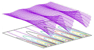
  $0.5$. Figure 4 shows the maximum value of the imaginary part
  $c_i$ of
  $c$ as a function of
  $\alpha$ and
  $R_\delta$ irrespective of the phase of the cycle at which the maximum takes place. The line characterized by
  $c_i=0$ is the marginal stability curve in the plane
  $(\alpha ,R_\delta )$.

Figure 4. The maximum values of  $c_i$ observed during the cycle, irrespective of the phase at which they are observed, plotted versus
  $\alpha$ and
  $R_\delta$.
Figure 5 shows the phase  $t_{ins}$ of the cycle at which the instability first occurs as a function of the Reynolds number. Close to the critical conditions, the instability is predicted close to
  $t={{\rm \pi} }/{2}+n {\rm \pi}$ with
  $n=0,1,2,\ldots$ but the instability takes place earlier as the Reynolds number is increased.

Figure 5. Phase  $t_{ins}$ of the cycle, at which instability first occurs, plotted versus the Reynolds number for
  $\alpha =0.5$. Similar results are obtained for different values of
  $\alpha$. Needless to say that the instability is predicted also at
  $t_{ins}+n{\rm \pi}$ with
  $n=0,1,2,\ldots$.
These results were already obtained by Blondeaux & Seminara (Reference Blondeaux and Seminara1979). However, Blondeaux & Seminara (Reference Blondeaux and Seminara1979) did not look at the behaviour of  $c$ for larger values of
  $R_\delta$. Figure 6 shows the imaginary part of
  $c$ as a function of
  $t$ for
  $\alpha =0.5$ and
  $R_\delta =500$ and
  $1500$. For the smallest value of
  $R_\delta$, there is a time interval during which even the most unstable mode is characterized by a negative value of
  $c_i$, implying a momentary decay of the perturbation. On the other hand, for
  $R_\delta =1500$, there is an unstable mode during the whole cycle. In figure 6, the points
  $D$ indicate the phase of the cycle such that the perturbation which propagates in the positive direction of the
  $x$-axis has the same growth rate as the perturbation which propagates in the negative direction. To determine the critical value
  $R_{\delta ,c3}$ which leads to the growth of perturbations at any phases of the cycle, the evaluation of
  $c_i$ is carried out for many values of
  $R_\delta$ and
  $\alpha$. Figure 7 shows the value
  $c_i$ at the point
  $D$ (see panel (b) of figure 6) plotted in the plane
  $(\alpha , R_\delta )$. Looking at figure 6, it can be realized that the instability pervades the whole oscillation cycle when
  $c_i$ at the point
  $D$ is zero or positive. It follows that the results plotted in figure 7 allow the determination of the value
  $R_{\delta ,c3}$ of the Reynolds number such that, for
  $R_\delta$ larger than
  $R_{\delta ,c3}$, a growing perturbation is present during the whole cycle. It turns out that
  $R_{\delta ,c3} = 818$ and the most unstable perturbation is characterized by the wavenumber
  $\alpha _{c,3} = 0.4$. Hence, it can be inferred that the fully turbulent regime is predicted by the present analysis when the Reynolds number is larger than
  $818$.

Figure 6. Imaginary part of the growth rate  $c$ for
  $\alpha =0.5$ and
  $R_\delta =500$ (continuous line) and
  $R_\delta =1500$ (dashed–dotted line). Panel (b) is an enlargement of panel (a).

Figure 7. Imaginary part  $c_i$ of the growth rate at the point
  $D$ (see figure 6) plotted versus
  $\alpha$ and
  $R_\delta$.
In figure 8, the value of  $c_i$ is plotted for
  $\alpha =0.5$ and different values of
  $R_\delta$. When the Reynolds number is not too far from
  $R_{\delta ,c1}$, the instability is restricted to small parts of the oscillatory cycle. However, when the Reynolds number is increased beyond
  $200$, the unstable time interval rapidly increases, and for
  $R_\delta \simeq 550$ the instability pervades a large part of the decelerating phases and the whole accelerating phases. Indeed, the lower limit
  $t_1$ of the unstable time intervals does not change significantly when the Reynolds number is increased, whereas the upper limit
  $t_2$ moves quickly to
  $2{\rm \pi}$. We remind the reader that
  $c_i(t-{\rm \pi} )=c_i(t)$ is also an eigenvalue which is not plotted in figure 8 for the sake of clarity. Hence, the instability phases also range between
  $t_1 \pm n {\rm \pi}$ and
  $t_2 \pm n {\rm \pi}$.

Figure 8. Imaginary part of the growth rate  $c$ for
  $\alpha =0.5$ and different values of
  $R_\delta$.
The existence of a further critical value of the Reynolds number  $R_{\delta ,c2}$ can be inferred, beyond which, not only a growing perturbation exists, but transition to turbulence is promoted during a large time interval. The different qualitative behaviour of the perturbations, when the Reynolds number moves from
  $200$ to
  $550$ and beyond, clearly appears when the values of
  $t_1$ and
  $t_2$, i.e. the boundaries of the unstable time intervals, are plotted versus the Reynolds number. Figure 9 clearly shows that, while
  $t_1$ decreases continuously with
  $R_\delta$,
  $t_2$ is characterized by a sudden and rapid growth when
  $R_\delta$ becomes larger than approximately
  $200$. The rapid growth of the unstable phases is more evident if
  $t_2$ and
  $d t_2/d R_\delta$ are plotted versus the Reynolds number. Indeed figure 10 shows that the value of
  $d t_2/d R_\delta$ decreases from large values to small values when
  $R_\delta$ moves from
  $85$ to
  $187.5$ but it suddenly jumps to larger values when
  $R_\delta$ moves from
  $187.5$ to
  $200$, and decays again for values of
  $R_\delta$ larger than
  $200$.

Figure 9. Value of the boundaries of the unstable time intervals during the oscillation cycle as a function of  $R_\delta$ (
 $\alpha =0.5$). A similar curve does exist with
  $t$ decreased by
  ${\rm \pi}$.

Figure 10. Value of  $t_2$ (a) and of
  ${\textrm {d}}t_2/{\textrm {d}}R_\delta$ (b) evaluated by means of a forward finite difference approximation of the data plotted in panel (a) for
  $\alpha =0.5$.
4. Conclusions
The present momentary stability analysis extends to the ‘infinite’ case the analysis of Von Kerczek & Davis (Reference Von Kerczek and Davis1974) who considered the ‘finite’ case, introducing a wall at a distance  $h$ from the oscillating wall which generates the Stokes boundary layer.
Even though the present results come from a linear analysis of the time development of perturbations of the Stokes boundary layer and, certainly, it cannot be claimed that they describe turbulence dynamics, the present findings explain the presence of the different flow regimes observed in the laboratory experiments (see, amongst others, Hino et al. (Reference Hino, Sawamoto and Takasu1976), Hino et al. (Reference Hino, Kashiwayanagi, Nakayama and Hara1983), Jensen et al. (Reference Jensen, Sumer and Fredsøe1989) and Akhavan et al. (Reference Akhavan, Kamm and Shapiro1991a)).
Indeed, the present results show the following.
(i) Perturbations of the laminar flow start to appear when  $R_\delta$ becomes larger than a value
  $R_{\delta ,c1}$ which is approximately
  $85$. This theoretical result provides an explanation of the laboratory observation of disturbances of the laminar regime which appear when the Reynolds number becomes larger than a value which depends on the experimental apparatus but ranges around
  $100$.
(ii) When the Reynolds number becomes larger than  $R_{\delta ,c1}$, but it stays smaller than approximately
  $200$, the instability is restricted to small parts of the oscillation cycle, close to the inversions of the velocity of the oscillating plate, from
  $t=t_1+n{\rm \pi}$ to
  $t=t_2+n{\rm \pi}$. This hydrodynamic regime can be paired with the ‘disturbed laminar’ regime.
(iii) When the Reynolds number is increased beyond  $200$ the range of unstable phases of the cycle rapidly increases until for
  $R_\delta =R_{\delta ,c2}\simeq 550$, the instability pervades a much larger part of the cycle and in particular the whole accelerating phases. In this range of the Reynolds number, the dynamics of the perturbations is expected to give rise to the ‘intermittently turbulent regime’.
(iv) Finally, when the Reynolds number becomes larger than  $R_{\delta ,c3} \simeq 850$, the instability spreads all over the cycle. Hence, turbulence is expected to be present during the whole cycle and the ‘fully turbulent’ regime to be observed (see the experimental measurements of Hino et al. (Reference Hino, Kashiwayanagi, Nakayama and Hara1983) and Jensen et al. (Reference Jensen, Sumer and Fredsøe1989)).
In figure 11, the results of the present analysis are plotted along with the data of Hino et al. (Reference Hino, Sawamoto and Takasu1976), who investigated the transition process in the oscillatory boundary layer which is generated in a pipe of circular cross-section. Hence, the flow regimes observed by Hino et al. (Reference Hino, Sawamoto and Takasu1976) depend not only on the Reynolds number but also on the ratio  $\lambda ={R^{*}}/{\delta ^{*}}$,
  $R^{*}$ being the radius of the pipe section. Even though different terms were used by Hino et al. (Reference Hino, Sawamoto and Takasu1976), namely (i) ‘laminar flow at low Reynolds numbers’, (ii) ‘weakly turbulent flow at transition Reynolds numbers’, (iii) ‘conditionally turbulence at higher Reynolds numbers’, the velocity signals plotted in figures 3, 4 and 6 of the paper of Hino et al. (Reference Hino, Sawamoto and Takasu1976) suggest that the flow regimes (ii) and (iii) can be associated with the disturbed laminar regime and intermittently turbulent regime, respectively. As expected, the results of the present stability analysis tend to provide a fair prediction of the flow regimes observed during the experiments of Hino et al. (Reference Hino, Sawamoto and Takasu1976) when
  $\lambda$ tends to be much larger than unity, even though further experiments would be necessary to fully support the theoretical analysis.

Figure 11. The different flow regimes observed in the boundary layer generated by an oscillatory flow in a pipe of circular cross-section plotted as a function of the Reynolds number and of the ratio  $\lambda ={R^{*}}/{\delta ^{*}}$,
  $R^{*}$ being the radius of the pipe section. White points, laminar flow regime; black points, disturbed laminar regime; black points with crosses, intermittently turbulent regimes. The dashed lines show the critical values of the Reynolds number predicted by the present linear stability analysis.
As already pointed out, nonlinear effects certainly affects the dynamics of the perturbations when their amplitude becomes large, and quantitative differences are expected to be present when the present results are compared with the experimental observations. Indeed, differences amongst the critical values of the Reynolds number predicted by the present stability analysis and those observed in the laboratory experiments are present. Nevertheless, the present results provide a physical insight into the mechanisms giving rise to the different flow regimes characterizing an oscillatory boundary layer. Only direct numerical simulations (DNS) can be used to follow the growth of the flow perturbations until they attain their mature stage (see, amongst others, Akhavan, Kamm & Shapiro (Reference Akhavan, Kamm and Shapiro1991b), Verzicco & Vittori (Reference Verzicco and Vittori1996), Vittori & Verzicco (Reference Vittori and Verzicco1998), Costamagna, Vittori & Blondeaux (Reference Costamagna, Vittori and Blondeaux2003) and Mazzuoli, Vittori & Blondeaux (Reference Mazzuoli, Vittori and Blondeaux2011)). In particular, Thomas et al. (Reference Thomas, Davies, Bassom and Blennerhassett2014) and Ramage et al. (Reference Ramage, Davies, Thomas and Togneri2020) made DNS of oscillatory Stokes layers and showed that perturbations of the laminar regime grow rapidly after the wall shear stress reverses its direction. However, because of the high computational costs, DNS do not allow a detailed investigation of the parameter space which would require a large number of simulations for different values of the Reynolds number ( $R_\delta$) and of the size of the computational domain (
 $\alpha$). Hence, the results of this linear stability analysis could help to select the numerical simulations to be made.
Acknowledgements
The authors are grateful to Professor G. Seminara for his comments and valuable suggestions.
Funding
This study has been partially supported by Ministero dell'Istruzione dell'Universitá e della Ricerca - MIUR (under grant FUNBREAK-PRIN2017 n. 20172B7MY9) and by the University of Genova.
Data availability statement
The data that support the findings of this study are openly available in OSF at https://osf.io/9hbgr/.
Author contributions
Both authors contributed equally in analysing data, reaching conclusions and in writing the paper.
Declaration of interests
The authors report no conflict of interest.


 Open access