


1. Introduction
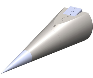
The flow field around a hypersonic body can involve many complex interactions. Flow deflection towards the free stream, such as that obtained by a compression corner, results in shock waves that interact with the upstream boundary layer, amplify disturbances and may even cause it to separate (Chapman, Kuehn & Larson Reference Chapman, Kuehn and Larson1958). However, flow deflection away from the free stream, such as that by an expansion corner, results in expansion fans and attenuation of disturbances in the boundary layer (Sternberg Reference Sternberg1954). This amplification or attenuation of disturbances affects the state of the boundary layer. Predicting this boundary-layer response along with shock-wave/boundary-layer interaction (SBLI) have been identified as two of the key scientific challenges towards the development of hypersonic vehicles (Leyva Reference Leyva2017). Detailed studies focusing individually on expansion and on compression corners have been carried out using two-dimensional canonical geometries in supersonic and hypersonic flow (Smits & Dussauge Reference Smits and Dussauge2006). However, as noted by Dolling (Reference Dolling2001), new studies on complex geometries are needed to bridge the gap between our understanding from canonical studies and the flow physics in real-world applications. To this end, a non-canonical geometry, as shown in figure 1, is the focus of the present work. This geometry is inspired by earlier designs used in previous suborbital (Martellucci & Weinberg Reference Martellucci and Weinberg1982; Oberkampf & Aeschliman Reference Oberkampf and Aeschliman1992; Walker & Rodgers Reference Walker and Rodgers2005) and orbital (Massobrio et al. Reference Massobrio, Viotto, Serpico, Sansone, Caporicci and Muylaert2007; Pezzella, Marino & Rufolo Reference Pezzella, Marino and Rufolo2014) hypersonic reentry-body studies.

Figure 1. Cone-slice-ramp geometry: (a) side view, expansion-only case; (b) iso view, expansion-compression case with a  $10^{\circ }$ ramp.
Interaction of a high-speed boundary layer with a two-dimensional compression ramp is a canonical SBLI geometry that has received considerable attention (Delery Reference Delery1985; Knight et al. Reference Knight, Yan, Panaras and Zheltovodov2003; Babinsky & Harvey Reference Babinsky and Harvey2011; Clemens & Narayanaswamy Reference Clemens and Narayanaswamy2014; Gaitonde Reference Gaitonde2015). The flow deflection subjects the upstream boundary layer to an adverse pressure gradient, and whether this imposed pressure gradient is enough to cause flow separation or not depends on the state of the boundary layer. The boundary-layer state is dependent upon a number of key variables such as the shape parameter, laminar sub-layer thickness and subsonic-layer thickness (Delery Reference Delery1985). Overall, a laminar boundary layer is highly susceptible to separation whereas a turbulent boundary layer has increased momentum in the near-wall region that enables it to withstand a stronger adverse pressure gradient (Beresh, Clemens & Dolling Reference Beresh, Clemens and Dolling2002; Arnal & Delery Reference Arnal and Delery2004). The susceptibility to separation for a boundary layer can be quantified by either the size of the separation zone for a given pressure gradient (larger for laminar) or by the smallest flow deflection angle, or the incipient angle, that provides the pressure gradient needed for separation (smaller for laminar). In addition, when a laminar boundary layer separates, a characteristic decrease in surface heating is observed, whereas a heating increase occurs for a turbulent boundary-layer separation (Arnal & Delery Reference Arnal and Delery2004).
Due to the importance of the state of the boundary layer in determining the SBLI characteristics, there have been several studies on interaction between a shock wave and a boundary layer that is neither laminar nor fully turbulent. Among these, the majority pertain to either a laminar-to-turbulent transitional boundary layer (Benay et al. Reference Benay, Chanetz, Mangin, Vandomme and Perraud2006; Sandham et al. Reference Sandham, Schülein, Wagner, Willems and Steelant2014; Murphree et al. Reference Murphree, Combs, Yu, Dolling and Clemens2021) or involve imposed modifications that enhance some scales in an upstream turbulent boundary layer (Hayakawa & Squire Reference Hayakawa and Squire1982; Barter & Dolling Reference Barter and Dolling1995). However, there have been limited SBLI studies with a boundary layer undergoing a reduction in turbulent fluctuations, such as that obtained downstream of an expansion corner (Chew Reference Chew1979). A geometry where this effect becomes important is a cone-cylinder-flare (axisymmetric two-dimensional tandem expansion–compression). Several studies have been carried out on this geometry; while the earlier studies were concerned with characterizing the overall flow field for the different boundary layer states (Dennis Reference Dennis1957; Schaefer & Ferguson Reference Schaefer and Ferguson1962; Gray Reference Gray1967; Wadhams et al. Reference Wadhams, Mundy, MacLean and Holden2008), the recent ones have focused on understanding the transition mechanisms in the laminar separated shear layer after the expansion (Paredes et al. Reference Paredes, Scholten, Choudhari, Li, Benitez and Jewell2022; Benitez et al. Reference Benitez, Borg, Paredes, Schneider and Jewell2023a,Reference Benitez, Borg, Scholten, Paredes, McDaniel and Jewellb). However, these studies did not systematically investigate the effect of expansion on the upstream boundary layer and how that affected the subsequent SBLI.
A prominent work that does look into these effects is the extensive experimental study by Zheltovodov, Shilein & Horstman (Reference Zheltovodov, Shilein and Horstman1993) on two-dimensional tandem-expansion–compression (also known as backward-facing ramp) geometries. Turbulent boundary layers, at a wide range of Reynolds numbers (Re) and at Mach numbers (M) of 2 to 4, were subjected to backward-facing ramps of angles  $8^\circ$ to
  $45^\circ$. The results showed an increase in the separation bubble size with increasing
  $M$ but an opposite trend with increasing Re. The former was attributed to the suppression of turbulence by the expansion fan whose strength increases with
  $M$, and the latter was attributed to the turbulent recovery that occurs faster with increasing Re. The study suggested an increase in the ‘fullness’ of the boundary layer due to acceleration across the expansion corner. One of these cases, at Mach 2.9 with a
  $25^\circ$ ramp, was computationally simulated by Fang et al. (Reference Fang, Yao, Zheltovodov, Li and Lu2015), who showed that while the outer part of the expanded boundary layer is accelerated, as was suggested by Chew (Reference Chew1979) and Zheltovodov et al. (Reference Zheltovodov, Shilein and Horstman1993), the inner layer is in fact retarded after the expansion corner. Recently, Huo et al. (Reference Huo, Yi, Zheng, Niu, Lu and Gang2022) (Mach 3.4) varied the length of the expansion region as well as the expansion and compression angles, and showed that the separation region in front of a compression ramp is larger when an upstream expansion is introduced.
Since the SBLI characteristics are dependent on the upstream boundary-layer state, it is important to review the studies on high-speed boundary layers interacting with an expansion corner alone. It is now understood that an expansion corner acts to stabilize a supersonic boundary layer through the cumulative effects of convex curvature of the streamlines (Bradshaw Reference Bradshaw1973; Wang, Wang & Zhao Reference Wang, Wang and Zhao2017), favourable pressure gradient (Wang et al. Reference Wang, Wang, Sun, Wang and Hu2020) and bulk dilatation (mean density change). For an incoming laminar boundary layer, this leads to suppression of instabilities, which, for the high Mach number and conical geometry considered in this work, are the Mack second-mode waves (Mack Reference Mack1984). Recent computational (Chuvakhov et al. Reference Chuvakhov, Egorov, Ilyukhin, Obraz and Fedorov2021) and experimental (Butler & Laurence Reference Butler and Laurence2021) works have shown that as the upstream second-mode waves decay, frequency-shifted instability waves begin to appear in the thicker boundary layer after the expansion corner. For turbulent boundary layers, the upstream mass-flow fluctuations can diminish by a factor of three downstream of an expansion corner (Goldfeld, Nestoulia & Shiplyuk Reference Goldfeld, Nestoulia and Shiplyuk2002). Previous studies using theory and velocity measurements (Dussauge Reference Dussauge1987; Smith & Smits Reference Smith and Smits1991; Arnette, Samimy & Elliott Reference Arnette, Samimy and Elliott1998; Tichenor, Humble & Bowersox Reference Tichenor, Humble and Bowersox2013) and computations (Sun, Hu & Sandham Reference Sun, Hu and Sandham2017; Teramoto, Sanada & Okamoto Reference Teramoto, Sanada and Okamoto2017; Nicholson et al. Reference Nicholson, Huang, Duan, Choudhari and Bowersox2021) have shown that bulk dilatation, which peaks in the expansion fan region (Teramoto et al. Reference Teramoto, Sanada and Okamoto2017), is the primary cause of disturbance reduction. The reduction of turbulent fluctuations in an expanded boundary layer is particularly strong in the small-scale, high-frequency regime (Dawson, Samimy & Amette Reference Dawson, Samimy and Amette1994; Arnette et al. Reference Arnette, Samimy and Elliott1998). Since such fluctuations are dominant in the near-wall region, structurally, this suggests a wall-normal gradient in turbulence modification.
In a seminal work, Sternberg (Reference Sternberg1954) proposed that an expanded boundary layer assumes a two-layered structure with a near-wall layer that undergoes relaminarization and an outer layer containing inactive ‘debris’ of large-scale structures from the upstream boundary layer. This near-wall layer has been visualized in the supersonic regime using schlieren (Sternberg Reference Sternberg1954; Viswanath, Narasimha & Prabhu Reference Viswanath, Narasimha and Prabhu1978) and recently using high-resolution planar laser scattering (Wang, Wang & Zhao Reference Wang, Wang and Zhao2016). Similar observations have also been made in the incompressible regime where boundary layers subjected to strong favourable pressure gradients demonstrate an inner laminar boundary layer with reduced interaction with the outer turbulent layer and reduced surface skin-friction coefficient (Narasimha & Sreenivasan Reference Narasimha and Sreenivasan1973; Warnack & Fernolz Reference Warnack and Fernolz1998; Bourassa & Thomas Reference Bourassa and Thomas2009). Under strong relaminarization effects, near-wall mean velocity profiles have even been shown to be approximated by Falkner–Skan or Blasius profiles (Warnack & Fernolz Reference Warnack and Fernolz1998; Goldfeld et al. Reference Goldfeld, Nestoulia and Shiplyuk2002).
In a review paper, Sreenivasan (Reference Sreenivasan1982) defined ‘relaminarization’ as a process rather than an end state, in which an ‘initially turbulent flow is rendered effectively laminar’. He further defined ‘laminarescence’ as an intermediate stage in this process where the flow deviates from fully turbulent behaviour to exhibit properties reminiscent of laminar flow without being purely laminar. The actual state of the flow within this process depends, among other things, on the imposed pressure gradient (strength of the expansion) and the disturbance environment. Following Sreenivasan (Reference Sreenivasan1982), the term ‘relaminarization’ has been used in the present work in a comprehensive sense to mean a process whose intermediate stages manifest as a reduction in near-wall turbulence levels or a regression to an earlier state of transition. The use of this term does not necessarily mean that the flow has become strictly laminar.
The two-layered boundary-layer structure, resulting from the relaminarization effects due to the expansion, typically recovers to a turbulent boundary layer further downstream. This recovery process takes longer at a lower Reynolds number (Goldfeld & Lisenkov Reference Goldfeld and Lisenkov1991). Mean pressure recovery to inviscid values occurs over a distance that scales with the expansion strength that is quantified by a hypersonic similarity parameter  $K = M_{\infty }\alpha$, where
  $\alpha$ is the corner angle (Stollery & Bates Reference Stollery and Bates1974; Lu & Chung Reference Lu and Chung1992). This recovery typically occurs within a few boundary-layer thicknesses (Dawson et al. Reference Dawson, Samimy and Amette1994). However, due to slower recovery of turbulent quantities and limited length of the test articles used in high-speed boundary-layer experiments, the recovery to equilibrium turbulence is typically not achieved (Goldfeld & Lisenkov Reference Goldfeld and Lisenkov1991; Arnette et al. Reference Arnette, Samimy and Elliott1998). For a minor expansion (Mach 2.7,
  ${\sim }4^{\circ }$ corner), Sun et al. (Reference Sun, Hu and Sandham2017) found that that the near-wall velocity deficit was sustained even after approximately 15 boundary-layer thickness downstream of the corner, and the turbulent kinetic energy in the outer-layer was lower than that of a flat-plate boundary layer. A boundary layer encountering a stronger expansion is expected to recover over an even longer streamwise distance. The two-layered structure of such relaminarizing boundary layers poses modelling challenges to the typical design tools that employ equilibrium turbulence models (Rumsey & Spalart Reference Rumsey and Spalart2009; Ranjan & Narasimha Reference Ranjan and Narasimha2017; Nicholson et al. Reference Nicholson, Huang, Duan, Choudhari and Bowersox2021).
The state of the boundary layer downstream of an expansion corner determines the nature of its interaction with a subsequent compression ramp. The expanded boundary layer has a near-wall velocity deficit that results in enhanced susceptibility to separation and, consequently, a larger mean separation length. This explains the experimental findings of Zheltovodov et al. (Reference Zheltovodov, Shilein and Horstman1993) and Huo et al. (Reference Huo, Yi, Zheng, Niu, Lu and Gang2022) on tandem expansion–compression geometries where larger separation regions were observed with stronger upstream expansions (larger  $K$). As Re increases, the recovery (or the re-transition process) of the expanded boundary layer is expedited (Goldfeld & Lisenkov Reference Goldfeld and Lisenkov1991), and the separation length decreases (Zheltovodov et al. Reference Zheltovodov, Shilein and Horstman1993; Xie et al. Reference Xie, Xiao, Wang and Yang2022). It should be noted that while these studies do elucidate many important aspects of the expansion–compression flow field, these have been restricted to supersonic Mach numbers (Mach 2 to 4). Furthermore, these two-dimensional studies, including those on the cone-cylinder-flare geometry (Gray Reference Gray1967), lack the complexities present in three-dimensional geometries (Panaras Reference Panaras1996; Gaitonde & Adler Reference Gaitonde and Adler2023). For example, the geometry considered in this study (figure 1) has a three-dimensional expansion corner upstream of a spanwise-finite compression ramp. These non-axisymmetric geometric features result in spanwise-varying pressure fields and separation and reattachment fronts (Vogel et al. Reference Vogel, Coder, Chynoweth and Schneider2019), and an overarching goal of this study is to understand how much of our understanding from existing two-dimensional studies can be transferred to this non-canonical geometry.
To this end, the geometry shown in figure 1 has been studied in the recent years in the Sandia Hypersonic Wind Tunnel (HWT) (Pandey et al. Reference Pandey, Casper, Spillers, Soehnel and Spitzer2020, Reference Pandey, Casper, Soehnel, Spillers, Bhakta and Beresh2021, Reference Pandey, Casper, Guildenbecher, Beresh, Bhakta, Dezetter and Spillers2022, Reference Pandey, Jirasek, Saltzman, Casper, Beresh, Bhakta, Denk, De Zetter and Spillers2023; Saltzman et al. Reference Saltzman, Pandey, Beresh, Casper, Bhakta, Denk, De Zetter and Spillers2023). Although studies on similar geometries have been conducted in a hypersonic setting before, these have either been restricted to the laminar regime or were only concerned with characterizing the overall flow field for varying transition locations (Martellucci & Weinberg Reference Martellucci and Weinberg1982; Oberkampf & Aeschliman Reference Oberkampf and Aeschliman1992; Walker & Oberkampf Reference Walker and Oberkampf1992; Tan et al. Reference Tan, Tu, Sun, Liu, Meng and Yang2017; Thome et al. Reference Thome, Reinert, Dwivedi and Candler2018; Vogel et al. Reference Vogel, Coder, Chynoweth and Schneider2019; McKiernan & Schneider Reference McKiernan and Schneider2021; Quintanilha & Theofilis Reference Quintanilha and Theofilis2021; Terceros & Araya Reference Terceros and Araya2021; White et al. Reference White, West, Rhode, Rieken, Erb, Lampenfield and Rodriguez2021; Sadagopan et al. Reference Sadagopan, Huang, Jirasek, Seidel, Pandey and Casper2023; Francis et al. Reference Francis, Dylewicz, Klothakis, Theofilis and Jewell2024; Nicotra et al. Reference Nicotra, Moy, Ritchie, Zhou, Bane and Jewell2024; Sadagopan & Huang Reference Sadagopan and Huang2024). As such, there is currently limited understanding on the evolution of hypersonic boundary-layer instabilities and turbulence and their effect in a three-dimensional expansion–compression geometry that is relevant to real-world applications.
The current study used several experimental campaigns to carry out characterization of this three-dimensional geometry in hypersonic flow. The decrease in fluctuations was quantified for a range of Re conditions on the expansion-only geometry in the absence of the downstream compression ramp. Once the phenomenon of boundary-layer relaminarization was established, its effect on the subsequent SBLI was evaluated for two different compression ramp angles. A remarkable effect of relaminarization is the enhanced susceptibility to separation that has been demonstrated for a scenario where separation was not expected for a turbulent boundary layer. Apart from elucidating this important engineering result, this study helps improve understanding of SBLI phenomena in such non-canonical geometries by allowing comparisons with the large body of knowledge obtained from simpler two-dimensional geometries. Furthermore, the experimental results presented here can be used as a challenging test case for the analytical and computational tools used in hypersonic vehicle design.
2. Experimental set-up
2.1. Sandia Hypersonic Wind Tunnel and test conditions
The Sandia Hypersonic Wind Tunnel (HWT) is a conventional blowdown-to-vacuum facility with an interchangeable system of nozzles and heater sections for the selection of a desired Mach number in the test section (Beresh et al. Reference Beresh, Casper, Wagner, Henfling, Spillers and Pruett2015). In this work, the Mach 8 system was used that has a 355.6 mm diameter axisymmetric test section. The tunnel employs a bottle farm that stores nitrogen (working fluid) at 689 MPa. A control valve between the high-pressure storage and the tunnel allows a  $P_0$ range of 1720–6890 kPa, and an in-line heater provides a
  $T_0$ range of 500–890 K. This provides a Reynolds number (Re) range from
  $3.3\unicode{x2013}20 \times 10^6\ {\rm m}^{-1}$. The noise level of the HWT is 3 %–5 %, quantified as the root mean square (r.m.s.) Pitot pressure between 0 and 50 kHz over the mean Pitot pressure (Casper et al. Reference Casper, Beresh, Henfling, Spillers, Pruett and Schneider2016).
2.2. Model and sensors
The test model, shown in figure 1, is a  $7^{\circ }$ half-angle slender cone with a base diameter of 127 mm. The cone has a hyperbolic cut at an offset of 45.7 mm (72 % of the base radius) from its axis. The axial length of the resulting horizontal slice is 144.9 mm and, at its aft-end, the slice has a provision to mount 50.8 mm long and 44.5 mm wide ramps of different deflection angles. In this work, first a flat plate (
 $0^{\circ }$ ramp) was used that provided a baseline case for evaluating the effect of streamwise expansion on the cone boundary layer. Ramps of
  $10^{\circ }$ and
  $30^{\circ }$ angle were then used to set up SBLIs of different strengths and the concomitant flow features. The origin was located at the slice-ramp corner and at midspan of the ramp with
  $(x,y,z)$ coordinates pointing in the downstream, slice-normal and spanwise directions, respectively. In this work, the coordinates have been non-dimensionalized using the distance of the cone-slice corner from the origin along the plane of symmetry, i.e.
  $(\bar {x},\bar {y},\bar {z}) = (x,y,z)/L$, where
  $L = 94.1$ mm. This model was mounted using a sting at the base of the cone, and all testing was done at zero angle of attack. Slight variations can occur in the angle of attack of the wind tunnel model when attempting to hold it nominally to zero. The impact of this was studied by deliberately setting an angle of
  $+/- 0.2^{\circ }$, from which it was found that the resulting changes in the peak frequency or the amplitude of the second-mode waves, though detectable, were too modest to influence the relaminarization effects discussed herein. The effects at turbulent conditions were negligible. The experiments reported in this paper were conducted over several different HWT campaigns with compatible measurement/visualization techniques.
Zheltovodov & Knight (Reference Zheltovodov and Knight2011) note that complex three-dimensional interactions can be understood by comparison with equivalent two-dimensional flows and as a combination of canonical interactions. To facilitate such comparisons with two-dimensional studies, the sensors used in this work have been placed along the plane of symmetry of this three-dimensional geometry. Two rows of sensor holes, offset on either side of the plane of symmetry by 3.2 mm, were used. One row has 1.8 mm diameter holes for mounting Kulite sensors and the other row has 3.8 mm diameter holes for mounting PCB, Schmidt–Boelter and shear-stress sensors. The holes on the ramp are at the same distance from the origin irrespective of the ramp angle. The hole locations and the sensors used in the experiments have been summarized in table 1. The sensors were mounted flush with the model surface and the sensor cables routed through the sting to the data-acquisition set-up outside the tunnel. The model base plate had holes that allowed the internal cavity to equilibrate with the low pressures in the HWT.
Table 1. Instrumentation locations (distances from origin) on the model with lines demarcating the sensors on the cone, slice and ramp. Here,  $\bullet$ denotes corresponding measurements were made.

The Kulite row had a combination of Kulite XCQ-062-30As or XCE-062-15As for measuring surface-pressure fluctuations with a 0–30 kHz bandwidth. The sensors have a vendor-reported uncertainty of 0.1 % of the full-scale output which corresponds to approximately 100 and 200 Pa for the  $-$15As and
  $-$30As, respectively. Precision Filters’ 28000 analog signal-conditioning system with a 28144 module was used to provide the excitation voltage to the sensors and also to low-pass filter (anti-alias) the signals. The digitization was carried out using an NI-PXI system with NI-6133 modules. The signals were low-pass filtered at 80 kHz and sampled at 500 kHz. Although these sensors operate in the absolute mode (no reference pressure needed), determination of the zero-bias voltage was needed which was facilitated by the pre-run pressures recorded by a Kulite ETL-79 placed in the test section. The linear sensitivities of the sensors were then used to calculate the surface pressures during the run.
A thin boundary layer typically found on the small-scale geometries in hypersonic wind-tunnel experiments is associated with high-frequency pressure fluctuations. In this work, PCB132B38 sensors that have a frequency bandwidth of 11–1000 kHz have been used that allow measurements of high-frequency pressure fluctuations in laminar (Fujii Reference Fujii2006) and turbulent boundary layers (Beresh et al. Reference Beresh, Henfling, Spillers and Pruett2011). These sensors have demonstrated success in previous HWT experiments on a straight-cone (Casper et al. Reference Casper, Beresh, Henfling, Spillers, Pruett and Schneider2016), and extend the measurements of the lower-frequency Kulite sensors to capture the second-mode waves and its higher harmonics. The sensor has an external diameter of 3.175 mm and a rubber sleeve was used to provide electrical insulation as well as to help isolate it from structural vibrations; the actual sensing-element diameter is 0.81 mm (Ort & Dosch Reference Ort and Dosch2019). The excitation was provided by a PCB 482A22 signal conditioning system and the anti-alias low-pass filtering was provided by Precision Filters’ 28612 module. The digitization was carried out using an NI-PXI system with NI-6396 modules. The signals were low-pass filtered at 2 MHz and sampled at 5 MHz.
In measurements of high-frequency, small-scale disturbances, spatial averaging effects due to the finite sensor size can cause unwanted attenuation of fluctuations (Corcos Reference Corcos1963; Beresh et al. Reference Beresh, Henfling, Spillers and Pruett2011). The attenuation model of Corcos (Reference Corcos1963), derived originally for the incompressible regime, has been shown to correct the PCB data of hypersonic boundary layers (Huang et al. Reference Huang, Duan, Casper, Wagnild and Bitter2024) using  $U_{c}/U_{e} = 0.8$, where
  $U_{c}$ is the convection velocity of the pressure fluctuation-inducing eddies and
  $U_{e}$ is the edge velocity. According to this model,
  $-$3 dB attenuation occurs for
  $\omega *r/U_{c} = 1$, where
  $\omega = 2{\rm \pi} f$ is the circular frequency,
  $r$ is the sensor radius and
  $U_{c}$ is the convection velocity of the pressure fluctuation-inducing eddies. The estimated
  $-$3 dB cutoff for the PCB measurements of the turbulent boundary layer on the cone is approximately
  $f=330$ kHz. To extend the PCB data up to 500 kHz, the Corcos correction has been applied to the turbulent dataset. For the laminar and transitional boundary layers, no correction was necessary since the dominant fluctuations, due to second-mode instability, exhibit frequencies of approximately 200 kHz or lower on this geometry.
Schmidt–Boelter gauges (Medtherm Corporation; 8-1-0.25-45-20835EBS) were used to measure the heat flux on the slice and the ramp. The gauges house a thermopile in a 2.79 mm diameter cavity with a thermocouple on each of its two ends (Sullivan et al. Reference Sullivan2012). The sensor has an external diameter of 3.175 mm and the same mounting procedure as the PCB was used. The sensor has a reported uncertainty of 3 %. The signals were low-pass filtered at 1 kHz and were sampled at 20 kHz.
Shear-stress measurements were carried out using novel miniature sensors (AH-125-02) developed by Ahmic Aerospace, LLC. The sensing element was a floating head that was connected to the base of the housing through a flexure connected to strain gauges. After calibration of the strain induced on the flexure, measurement of shear stress on the floating head can be made (Meritt & Schetz Reference Meritt and Schetz2016; Meritt et al. Reference Meritt, Schetz, Marineau, Lewis and Daniel2017). The sensing element and the external housing are 2.41 mm and 3.175 mm in diameter, respectively. The sensor can measure shear stress up to 150 Pa with a reported uncertainty of 0.75 Pa at a rate of approximately 250 Hz. The signals were low-pass filtered at 1 kHz and sampled at 20 kHz.
2.3. High-frame-rate schlieren and focused laser differential interferometry
In addition to the sensor measurements, flow-visualization and off-surface density fluctuations were captured using schlieren and focused-laser-differential interferometry (FLDI). Both these techniques were qualitative in nature but provided useful insights into boundary-layer growth and the relaminarization phenomena.
The high-frame-rate schlieren system incorporated an incoherent pulsed laser (Cavilux Smart) and a camera (Phantom v2512 or Phantom TMX7510). The laser generated pulses of 10 ns duration at high repetition rates, either 100 kHz for 10 s or 465 kHz for bursts of 4 to 5 ms. The  $z$-type schlieren configuration used two 450.8 mm diameter, 2.75 m focal length, spherical mirrors for light-collimation and a knife edge oriented horizontally to resolve vertical gradients in density (Settles Reference Settles2001). The schlieren system provided a spanwise-integrated visualization of the boundary layer and SBLI. Two sets of data were acquired over different wind tunnel entries. The first set used a Phantom v2512 at 100 kHz with a
  $640 \times 208$ pixel area that captured the whole slice-ramp region with a resolution of
  $2.56\ {\rm pixels}\ {\rm mm}^{-1}$. The second set used a Phantom TMX7510 at 465 kHz with a
  $1280 \times 64$ pixel area to capture the boundary-layer evolution of the expansion-only case with a resolution of
  $7.67\ {\rm pixels}\ {\rm mm}^{-1}$.
To measure the high-frequency disturbances in the turbulent boundary layer, a scanning-FLDI system has been used. A typical FLDI system consists of two sides that reside across the test section; an FLDI beam pair is generated on the first side and, after passing through the measurement region and encoding the density gradient information, is received on the other side (Smeets Reference Smeets1972; Parziale, Shepherd & Hornung Reference Parziale, Shepherd and Hornung2013). The focusing aspect of FLDI ensures that the beam pair is only sensitive to a finite region near the point of focus (Schmidt & Shepherd Reference Schmidt and Shepherd2015). The scanning-FLDI used two mirrors on either side to fold the traditional FLDI set-up, which was then mounted on a horizontal stage that traversed along the wind-tunnel axis. The scanning-FLDI probe was focused at the plane of symmetry and scanned the boundary layer 3.5 mm above the slice surface at  $14\ {\rm mm}\ {\rm s}^{-1}$. A Coherent Verdi laser set at 50 mW output power was used as the light source. The first side consisted of a 25 mm plano-concave lens (Edmund Optics 47911) that expanded the laser beam, a linear polarizer (ThorLabs LPVISA100) and a 2-arcminute Wollaston prism (United Crystals) that split the beam into a diverging beam pair. A 200 mm achromat lens (Edmund Optics 88593) followed by a 532-nm mirror focused the beam pair at the centreplane. A beam profiler measured the resulting beam diameters to be 0.03 mm with a spacing of 0.1 mm. The optics on the other side were symmetrical with a photodetector (ThorLabs PDA10A2) replacing the expanding lens to measure the interference between the beam pair. The photodetector signal was coupled to the data acquisition system using AC coupling; the signal was low-pass filtered at 2.5 MHz and digitized at 5 MHz. Further details and pictures can be found from Pandey et al. (Reference Pandey, Casper, Guildenbecher, Beresh, Bhakta, Dezetter and Spillers2022).
2.4. Oil-flow visualization and temperature-sensitive paint
To visualize the three-dimensionality of the flow field, oil flow and temperature-sensitive paint (TSP) were used. Oil-flow visualization provided surface streaklines (which align with streamlines in steady flow) on the geometry which were useful in verifying flow symmetry as well as in identifying separation and reattachment locations. A thin coating of low-viscosity fluorescent liquid (Zyglo ZL-15) was sprayed on the model prior to the run. Over the course of the run, the streakline pattern settled with a settling time of 1 to 15 s depending upon the flow conditions. It was illuminated using UV lights and the slice-ramp region was captured by a LaVision sCMOS camera at a resolution of  $15.1\ {\rm pixels}\ {\rm mm}^{-1}$.
TSP was used to visualize the heating pattern on the model and provide an additional diagnostic for the extent of the SBLI separation region. The TSP formulation used was Ru(bpy) in a clearcoat (Liu & Sullivan Reference Liu and Sullivan2005). The paint was excited with 460 nm water-cooled lights (ISSI LM2XX-400). Images were acquired with a LaVision sCMOS camera at a resolution of  $6.8\ {\rm pixels}\ {\rm mm}^{-1}$. A 550 nm high-pass filter was used to remove the excitation light and capture only the paint emission. The temperature measured by TSP was converted to heat flux using an in situ scaling method used in previous studies (Sullivan et al. Reference Sullivan2012; Liu et al. Reference Liu, Ward, Rubal, Sullivan and Schneider2013; Juliano, Borg & Schneider Reference Juliano, Borg and Schneider2015). A scale factor was computed by using a linear fit between the heat-flux obtained from a Schmidt–Boelter gauge, located on the slice (
 $x = -49.9$ mm), and the temperature obtained from TSP near the gauge. Under the assumption that the paint characteristics are similar and the heating effects are linear, this scale factor was then applied to the whole TSP image to estimate the full-field heat flux. Although the accuracy of this scaling method is limited further away from the gauge location (Juliano et al. Reference Juliano, Borg and Schneider2015), salient differences in the heating patterns of laminar/transitional and fully turbulent SBLIs are much greater than the estimated errors in the heat-flux fields.
3. Effect of expansion on the boundary layer
The boundary layer developing on the upstream cone region of the current geometry undergoes an abrupt expansion as it encounters the slice corner. The effect of this three-dimensional feature on the mean flow field is first discussed for the expansion-only geometry, as shown in figure 1(a). The evolution of the boundary-layer disturbances is then discussed in the context of high-frequency experimental measurements that describe the relaminarization behaviour on this geometry. A range of Reynolds numbers was used to examine stabilization across different boundary-layer states.
3.1. Mean flow
The two-dimensional expansion-corner studies, reviewed in § 1, use expansion ramps, such as were used by Dussauge (Reference Dussauge1987), or an axisymmetric cone-cylinder geometry, such as was used by Sternberg (Reference Sternberg1954), to subject the upstream boundary layer to an expansion. In contrast, the current cone geometry has a hyperbolic cut that results in a curved expansion edge and a spanwise finite region of low pressure. The goal of this section is to assess the effect of this three-dimensional relief on the cone boundary layer and how it compares with two-dimensional studies.
Figures 2(a) and 2(b) show instantaneous surface oil-flow visualization for a laminar and a turbulent upstream boundary-layer state, respectively. The two cases show qualitative similarity except that for the higher Re case, the oil spreads quickly into smooth surface streaklines presumably due to larger surface shear. A few oil flow streaklines have been indicated using black dashed curves in panel (b). The streakline on the plane of symmetry moves straight from the cone onto the slice without any deviation or interruption, verifying that there is no flow separation due to the  $7^{\circ }$ expansion. Cone streaklines azimuthally away from the plane of symmetry appear to follow the expected diverging trajectory on the cone until they approach the slice where the low pressure on the slice attracts the fluid and causes spanwise-inward turning of the streaklines. Further downstream on the slice, these streaklines begin to diverge away from the plane of symmetry suggesting development of secondary flow. Despite this opposing outward flow, cone streaklines continue to climb onto the slice even at the end of the model.

Figure 2. Oil-flow visualization for (a) a laminar case  $Re = 4.7 \times 10^6\ {\rm m}^{-1}$ and (b) a turbulent case
  $Re = 16.2 \times 10^6\ {\rm m}^{-1}$ on the cone-slice expansion configuration. Black dashed curves in panel (b) track a few streaklines.
As documented by two-dimensional studies, flow expansion leads to thickening of the boundary layer; for example, Arnette et al. (Reference Arnette, Samimy and Elliott1998) found that for a Mach 3 free stream, boundary-layer thickness increased by a factor of 1.5 and 2 across  $7^{\circ }$ and
  $14^{\circ }$ expansions, respectively. This expansion of the boundary layer is apparent in figure 3 that shows ensemble averaged (50k images) schlieren images for a laminar and a turbulent case. The mean density gradients in the boundary layer appear as increased intensity in the image. The thickening is strongest across the expansion fan which is visible as a region of increased schlieren intensity emanating from the cone-slice corner into the free stream. Expansion fans are regions of increased bulk dilatation and are bounded by Mach waves. Here, the cone edge Mach number estimated using Taylor–Maccoll equations and a slice Mach number estimated using inviscid two-dimensional Prandtl–Meyer equations have been used to obtain the two Mach waves shown in the figure (dashed lines). The intensity gradient in the free stream at the start of the expansion fan corresponds well with the first Mach wave.

Figure 3. Mean schlieren visualization. Whites dots trace the extracted boundary layer edge and dashed lines approximately bound the expansion fan region in the plane of symmetry: (a)  $Re = 4.7 \times 10^6\ {\rm m}^{-1}$; (b)
  $Re = 16.2 \times 10^6\ {\rm m}^{-1}$.
The white dots in figure 3 track the boundary-layer edge educed from the averaged schlieren images. While the  $z$-type schlieren implemented here provides a spanwise-integrated side view of the boundary layer development, it can be argued that the extracted edge represents the boundary layer edge in the plane of symmetry since the expansion occurs there first. For the laminar case shown in figure 3(a), the r.m.s. schlieren intensity clearly helps demarcate the edge of the boundary layer. For the turbulent case shown in figure 3(b), the edge has been defined as the wall-normal location at which the double-derivative of the schlieren intensity value peaks; this identifies the location where the schlieren intensity begins to increase sharply. The extracted edge appears to faithfully capture the growth of the boundary layer in figure 3.
Streamwise pressure gradient is an important parameter that affects the boundary layer stabilization. To quantify it, the mean (temporally averaged) pressures measured by the Kulite transducers are shown in figure 4. For a few locations, uncertainty bars are shown that correspond to the vendor-reported value of 0.1 % of full-scale output. As Re increases, mean pressure values increase and the relative uncertainty magnitudes decrease. To normalize the data, estimates of pressure upstream of the expansion corner have been obtained using the Taylor–Maccoll equations that provide the cone-edge pressure ( $P_{{CE}}$). In addition, inviscid estimates of pressures downstream of a two-dimensional,
  $7^{\circ }$ expansion corner have been obtained using the Prandtl–Meyer equations (
 $P_{{PM}}$). Figure 4(a) shows that this allows reasonable collapse of data across several different Reynolds numbers considered here. Also shown are measurements by Oberkampf et al. (Reference Oberkampf, Aeschliman, Henfling and Larson1995) who used a
  $10^{\circ }$ blunt cone geometry with a similar slice-length to cone-length ratio of 30 %, although the cone length was considerably shorter (264 mm as compared to 517 mm of the current geometry). The abscissa has been normalized by the length of the full slice (
 $L_{{slice}}$) in the plane of symmetry from the cone-slice corner to the base of the geometry. The results show that the upstream pressure on the cone is close to the edge value predicted by the Taylor–Maccoll equation but the pressure on the slice (in the plane of symmetry) is not well represented by the two-dimensional inviscid estimate.

Figure 4. Normalized mean pressure. (a) Comparison at several Reynolds numbers, Re indicated as  $\times 10^6\ {\rm m}^{-1}$. For clarity, exemplar uncertainty bars are shown for only a few locations. (b) Turbulent case compared with previous two-dimensional expansion corner studies.
The turbulent case ( $Re = 16.5 \times 10^6\ {\rm m}^{-1}$) is compared with data from turbulent two-dimensional expansion corner literature in figure 4(b). The streamwise dimension has been normalized using the upstream boundary layer thickness (
 $\delta _0$) and the hypersonic similarity parameter (
 $K \equiv M_{\infty }\alpha$, where
  $\alpha$ is the corner angle in radians). The boundary-layer edge extracted at
  $\bar {x} = -1$ from the mean schlieren image shown in figure 3(b) was used as
  $\delta _0$ for the current work. As suggested by Lu & Chung (Reference Lu and Chung1992), data across the two-dimensional studies show reasonable collapse with a pressure minimum that is within 5 %–10 % of the inviscid estimates achieved in a response length of 10–20 non-dimensional boundary layer thicknesses. However, the pressure decrease is not as strong in the current geometry and begins to plateau at approximately 20 % of the two-dimensional value. This suggests that the three-dimensional relief and the resulting flow field generate a pressure field on the slice that is different than a canonical two-dimensional expansion.
3.2. Boundary layer disturbances
Boundary-layer transition on a sharp-straight-cone geometry of the same length as the current geometry has been studied in the HWT at Mach 8 by Casper et al. (Reference Casper, Beresh, Henfling, Spillers, Pruett and Schneider2016). The study showed that for  $Re < 5.5 \times 10^6\ {\rm m}^{-1}$, transition does not occur on a 517 mm long,
  $7^{\circ }$ cone, but it moves significantly upstream of where the cone-slice corner is located on the current geometry (317.3 mm from the nose) for
  $Re > 13.0 \times 10^6\ {\rm m}^{-1}$. By varying the free stream Re, this study looks at the effect of the expansion on laminar, transitional and turbulent boundary layers.
The effect of Re variation is shown in figure 5 for four representative boundary-layer states using instantaneous schlieren images. The boundary-layer thickness, obtained from ensemble-averaged schlieren image, has been annotated using white dots in each image. At low Re shown in figure 5(a), the boundary layer is laminar and no disturbance is visible except occasional passage of instability wavepackets; one such packet has been annotated in the figure using a black arrow. A further increase in Re, as shown in figure 5(b), increases the prevalence of such instability waves while the boundary layer is still laminar. Figure 5(c) shows a transitional case where turbulent spots appear in the upstream cone boundary layer and on the slice and figure 5(d) shows a turbulent case where upstream boundary layer also appears turbulent.

Figure 5. Instantaneous schlieren visualization. White dots trace the extracted boundary layer edge from the mean image: (a)  $Re = 4.7 \times 10^6\ {\rm m}^{-1}$; (b)
  $Re = 6.2 \times 10^6\ {\rm m}^{-1}$; (c)
  $Re = 9.8 \times 10^6\ {\rm m}^{-1}$; (d)
  $Re = 16.2 \times 10^6\ {\rm m}^{-1}$.
It should be noted that due to the spanwise-integrated nature of the schlieren, figure 5 presents an amalgamated view of boundary-layer disturbances that may originate at different azimuths on the cone and then climb onto the slice due to the spanwise flow seen in figure 2. As such, analysis of turbulent structures on the slice is not possible. However, based on an understanding from previous studies (Arnette, Samimy & Elliott Reference Arnette, Samimy and Elliott1995), it can be expected that the size of the turbulent structures increases on the slice in accordance with the boundary-layer thickness. Furthermore, if a near-wall laminarescent layer exists on the slice, as seen in planar visualizations by Wang et al. (Reference Wang, Wang and Zhao2016), it will be camouflaged by the spanwise integration. However, the evidence for such near-wall relaminarization is presented next in the context of sensor measurements in the plane-of-symmetry for the different boundary-layer states.
3.2.1. Laminar regime
The second-mode waves are the dominant instability mechanism of a high-Mach-number boundary layer on a straight cone (Mack Reference Mack1984). The rope-like structures in figure 5(b) are a visual manifestation of these trapped acoustic waves that propagate downstream while resonating between the peaks in acoustic impedance at the wall and at the sonic line (Fedorov Reference Fedorov2011). The PSD of 1 s of PCB data is shown in figure 6 for  $Re = 5.9 \times 10^6\ {\rm m}^{-1}$. The sensor on the cone (
 $\bar {x}<-1$) shows the existence of strong second-mode waves at approximately 200 kHz and its higher harmonics. Narrow peaks in the high-frequency regime are due to electronic noise. A broadband decrease in pressure fluctuations occurs on the slice as shown by the sensor located less than 6 mm downstream (at
  $\bar {x} = -0.94$) of the corner. Further along the slice, pressure fluctuations in the high-frequency regime (>120 kHz) decrease strongly (annotated by a dotted arrow); at
  $\bar {x} = -0.53$, the second-mode amplitude is smaller than that on the cone by over two orders of magnitude. Further downstream, as the overall upstream second-mode energy decreases, a secondary peak at a frequency lower than the original second-mode peak appears (the two peaks have been annotated using double solid arrows). At lower frequencies (<100 kHz), the pressure fluctuations begin to increase on the slice. A small peak is seen to first appear at
  $\bar {x} = -0.53$ that becomes prominent and moves to lower frequencies in the downstream direction (annotated by a dashed arrow).

Figure 6. PSD of pressure fluctuations measured by PCBs for  $Re = 5.9 \times 10^6\ {\rm m}^{-1}$. Arrows show evolution of pressure-fluctuation peaks and are discussed in the text.
The frequency (  $f$) of second-mode waves observed in experiments scales as
  $f\delta /U_{e} = K$, where
  $\delta$ and
  $U_{e}$ are the local boundary-layer thickness and edge velocity, respectively, and
  $K$ is a constant (Stetson et al. Reference Stetson, Thompson, Donaldson and Siler1983; Marineau et al. Reference Marineau, Grossir, Wagner, Leinemann, Radespiel, Tanno, Chynoweth, Schneider, Wagnild and Casper2019). Across an expansion corner, the edge velocity does not change much;
  $U_{e}$ was estimated on the cone and the slice using Taylor–Maccoll equations and Prandtl–Meyer equations, respectively, and was found to vary by only 4 %. This implies that the frequency of the second-mode wave is inversely related to the boundary-layer thickness (Chuvakhov et al. Reference Chuvakhov, Egorov, Ilyukhin, Obraz and Fedorov2021), which is consistent with the concept of trapped acoustic waves.
Frequency peaks have been identified from the PSD data for the two laminar cases and are shown in figure 7(a). The uncertainty bars represent the frequency band associated with a  $5\,\%$ variation in peak amplitude (on both sides of the peak) to provide a measure of the uncertainty in peak identification. The high-frequency (180–250 kHz) peaks corresponding to the upstream second-mode waves have been identified until
  $\bar {x} = -0.53$, after which the dominant peak shifts to the low-frequency range (50–170 kHz). As seen in figure 6, these lower frequency peaks decrease in frequency towards the base of the cone. Using the local boundary-layer thickness (
 $\delta$) from schlieren, peak frequencies were non-dimensionalized and are presented in figure 7(b). Uncertainty bars were computed by combining the uncertainty bars in frequency peaks and the uncertainty in boundary-layer thickness estimation. The local value of
  $f\delta$ has been normalized by the value upstream on the cone
  $(f\delta )_{cone}$. Just downstream of the corner, the non-dimensional number
  $f\delta$ increases sharply due to rapid expansion of the boundary layer while the peak frequency corresponding to the attenuating upstream second-mode waves stays constant. However, further downstream,
  $f\delta$ realigns to the upstream value for both the Reynolds number cases suggesting that the increase in lower frequency energy is due to lower-frequency second-mode waves amplified by the thickened boundary layer. For non-dimensional
  $f\delta$ to correspond to 1 at
  $\bar {x} = -0.53$, the local boundary-layer thickness yields a peak second-mode frequency estimate of approximately 85 kHz (star symbol in figure 7). This corresponds well with the lower-amplitude local peak observed in the PSD data at
  $\bar {x} = -0.53$ in figure 6; at this location, the amplitude of the decaying second-mode waves from the cone remains larger than the new ones forming on the slice. These behaviours of the normalized frequency of the new instability wave are consistent with a second-mode wave developing under the thickened boundary layer.

Figure 7. Frequency peaks in the laminar regime at two Reynolds numbers. (a) Identified peaks. (b) Non-dimensionalized by the local boundary layer thickness. Circles are the measured peaks and stars are the estimated peaks. Black dashed lines represent the start and the end of the slice. Re in  $\times 10^6\ {\rm m}^{-1}$.
In addition to the PSDs, a time-domain analysis of the PCB data provides further insight into the nature of these instability waves. The cross-correlations across two sensors on the cone and on the slice are shown in figure 8 for 1 s of PCB data. The overall delay between the two sensors is smaller on the cone due to the close proximity of the sensors. The maximum and minimum in the correlation coefficients have been marked with red circles and the temporal gap between the two has been used to compute the dominant frequency. Figure 8(a) shows the archetypal wavepacket nature of the second-mode waves (Casper, Beresh & Schneider Reference Casper, Beresh and Schneider2014). The obtained frequency of 195 kHz corresponds well with that observed in figure 6. On the slice, the periodic nature of the wavepacket is still observed (figure 8b) although the cross-correlation is not as symmetric, presumably due to the incipient nature of the second-mode waves as well as larger distance between the sensors. However, the dominant frequency of 48 kHz compares well with the low-frequency peak at the last sensor at  $\bar {x} =0.40$ and provides further evidence for the instability-wave origin of this peak.

Figure 8. Cross-correlation between PCBs for  $Re = 5.9 \times 10^6\ {\rm m}^{-1}$: (a)
  $\bar {x} = -1.13$ and
  $\bar {x} = -1.06$; (b)
  $\bar {x} = 0.06$ and
  $\bar {x} = 0.40$. Red circles identify the maximum and minimum in the cross-correlation used to compute the frequency.
This emergence of lower-frequency second-mode waves is in agreement with two recent studies at Mach 6. Chuvakhov et al. (Reference Chuvakhov, Egorov, Ilyukhin, Obraz and Fedorov2021) performed linear stability analyses and DNS on two-dimensional  $5^{\circ }$ and
  $10^{\circ }$ expansion corners, and demonstrated that after the expansion, there do not exist any new modes of instability but only the second-mode wave at a lower frequency that is commensurate with the thicker boundary layer. Butler & Laurence (Reference Butler and Laurence2021) provided experimental verification for this on a
  $5^{\circ }$ cone-cylinder expansion and observed frequency-shifted, second-mode waves through spectral analysis of the schlieren visualizations. For the three-dimensional expansion geometry considered here, oil-flow streaklines in figure 2 confirm that the flow along the plane of symmetry is nominally straight and does not exhibit any cross-flow. Lack of cross-flow rules out the presence of travelling cross-flow instability as the source of frequency peaks after the expansion. Based on these findings, it is concluded that the low-frequency peaks in figure 6 correspond to the second-mode instabilities that are amplified on the slice at a frequency commensurate with the expanded boundary-layer thickness. More importantly, the decay of the upstream strong second-mode waves capable of inducing transition and their replacement by nascent waves of considerably smaller amplitude points to the transition-delaying ability of the expansion corner.
3.2.2. Transitional regime
As the Reynolds number is increased, transition of the boundary layer progresses further upstream along the cone. Figure 9 shows PSD of pressure fluctuations captured by the PCB sensors for two transitional Re cases; figure 5(c) is a representative schlieren image for this scenario. Comparing the PSD of the sensor at  $\bar {x}=-1.13$ across figures 9(a) and 9(b) shows that with increasing Re, the second-mode peak looses prominence and the pressure fluctuations on the cone become broadband. This is consistent with previous sharp-cone studies at Mach 8, which showed that boundary-layer transition occurs by first saturation, and then breakdown, of the second-mode waves (Stetson et al. Reference Stetson, Thompson, Donaldson and Siler1983; Casper et al. Reference Casper, Beresh, Henfling, Spillers, Pruett and Schneider2016). Narrow peaks in the PSDs are due to electronic noise, and sharp edges at 300 kHz and higher frequencies are due to sensor resonances (Ort & Dosch Reference Ort and Dosch2019).

Figure 9. PSD of pressure measured by PCBs: (a)  $Re = 9.4 \times 10^6\ {\rm m}^{-1}$; (b)
  $Re = 10.8 \times 10^6\ {\rm m}^{-1}$. Arrows show evolution of pressure-fluctuation peaks and are discussed in the text.
On the slice, akin to the laminar case (figure 6), the sensor just downstream of the cone-slice corner shows reduction in pressure fluctuation energy across all frequencies. The saturated second-mode peak loses its amplitude further as shown using a dotted arrow. Further downstream ( $\bar {x}>-0.5$), the flat spectrum gives way to a single dominant broad spectral peak in the 80–170 kHz range that shifts to lower frequencies like the laminar case. This has been annotated using a solid arrow in figure 9(b). The right (high-frequency) shoulder of this peak is associated with a dramatic decrease in the high-frequency fluctuations with a very steep roll-off that is reminiscent of prominent second-mode peaks in the laminar regime. The left (low-frequency) shoulder also shows smaller fluctuations than the broadband PSD of the upstream sensor at
  $\bar {x}=-0.94$. Cross-correlations of the time series signals confirmed that these broad peaks indeed correspond to second-mode waves; this is explored in detail in the next subsection for a turbulent boundary layer.
3.2.3. Turbulent regime
Two-dimensional studies in the supersonic regime have suggested that an expanded turbulent boundary layer shows behaviour of a two-layered boundary layer with a near-wall laminarescent layer and an outer turbulent layer with structures arriving from the upstream boundary layer (Sternberg Reference Sternberg1954). To quantify if such a behaviour occurs here, the surface pressure spectrum has been used to understand the contributions from the different parts of the boundary layer (Bull Reference Bull1996; Blake Reference Blake2017). The surface pressure spectrum for a hypersonic turbulent boundary layer has dominant energy near  $f \approx U_{\infty }/\delta$ (Duan, Choudhari & Zhang Reference Duan, Choudhari and Zhang2016), which corresponds to approximately 300 kHz for the boundary layer on the cone. The PCB measurements extend to more than twice this frequency (800 kHz) and are expected to capture the majority of these fluctuations. However, the spatial averaging effect due to the finite sensor size of the PCB causes attenuation at high frequencies. The Corcos correction (Corcos Reference Corcos1963; Huang et al. Reference Huang, Duan, Casper, Wagnild and Bitter2024) described in § 2.2 has been implemented to counter the spatial attenuation effects up to 500 kHz. The same correction factors have been used across all sensors, on the cone and along the slice, under the assumption that
  $U_{c}/U_{e}$ does not vary significantly across the expansion.
Figure 10(a) shows the PSD of 1 s of PCB data for a high-Re case. The sensor on the cone confirms the broadband nature of the upstream turbulent boundary layer; a few sharp peaks at 300 kHz and higher frequencies are due to sensor resonances and electronic noise. The rapid expansion downstream of the corner uniformly diminishes fluctuations across all scales as seen in the spectra at  $\bar {x} = -0.94$ and downstream. This reduction is in agreement with the mean pressure decrease shown in figure 4. Further downstream, the high-frequency fluctuations (>300 kHz) attenuate strongly such that at
  $\bar {x} = -0.53$ (
 ${\approx }13\delta _0$ downstream of corner), the fluctuations are 1–2 orders of magnitude smaller. By
  $\bar {x} = -0.13$ (
 ${\approx }24\delta _0$), a further decrease in high-pressure fluctuations is observed and the high-frequency roll-off begins at an even lower frequency. In fact, the pressure spectrum for
  $\bar {x} > -0.13$ in this turbulent case (
 $Re = 16.5 \times 10^6\ {\rm m}^{-1}$) has qualitative similarity to the transitional case (
 $Re= 10.8 \times 10^6\ {\rm m}^{-1}$) shown in figure 9(b). The spectra show a broad plateau with a high-frequency roll-off starting at approximately 200 kHz and a small peak in the 80–130 kHz range with a more gradual roll-off in the low-frequency regime. A slight shift of the spectral peak and the right shoulder towards lower frequencies can also be observed akin to the transitional case, corresponding to an expanding boundary layer. However, unlike figure 9(b), the left (lower-frequency) shoulder makes a recovery with increasing fluctuation values along the slice suggestive of broadband turbulent fluctuations.

Figure 10. (a) PSD of pressure fluctuations measured by PCBs for  $Re= 16.5 \times 10^6\ {\rm m}^{-1}$. (b) Zoom-in to show the frequency peaks. Spectra in panel (b) shifted down for clarity by multiplying the PSDs of the sensors at
  $\bar {x}=-0.53, -0.13, 0.06, 0.40$ by a factor of
  $1, 0.6, 0.3, 0.1$, respectively. Solid arrows in panel (b) point at peaks obtained from cross-correlation and dashed arrow in panel (b) annotates the leftward shift of the peak.
The frequency-dependence of the decrease in pressure fluctuations is explored in figure 11 using r.m.s. values obtained by integrating the pressure spectrum in discrete frequency bands. The r.m.s. pressure in each band ( $p'_{{rms}}$) has been normalized by the upstream value on the cone (
 $p'_{{rms\ cone}}$) in figure 11(a) and the results clearly show that the fluctuations are diminished across all frequencies with particularly strong attenuation in the high-frequency bands. The uncertainty bands in the figures represent the reported sensor uncertainty. It should be noted that although the PSD and the absolute r.m.s. values are dependent on the correction factors used for the Corcos correction, the r.m.s. ratios presented in figure 11 are not. This is because the comparison between the cone and the slice sensors have been made across consistent frequency bands that suffer the same attenuation effects.

Figure 11. (a) R.m.s. of pressure fluctuations measured by PCBs in several frequency bands for  $Re = 16.5 \times 10^6\ {\rm m}^{-1}$, (b) normalized by mean pressure at corresponding locations.
The decrease in the r.m.s. ratio (on the slice versus on the cone) is in agreement with the two-dimensional study at Mach 3 by Dawson et al. (Reference Dawson, Samimy and Amette1994), although measurements in that study were restricted to only 60 kHz. The particularly strong attenuation in the high-frequency regime points to the quenching of upstream small-scale, near-wall turbulent fluctuations. To assess if the local fluctuation levels are in fact lower on the slice, the r.m.s. values have been normalized by the mean pressure in figure 11(b). Here,  $P$ and
  ${P_{cone}}$ represent the mean local and cone pressures, respectively. Based on the integrated measurements from 1–60 kHz, Dawson et al. (Reference Dawson, Samimy and Amette1994) concluded that the fluctuation levels post-expansion do not decrease if normalized by the decreasing mean pressure. The results in figure 11(b) in the lower-frequency regime (<200 kHz) are consistent with this claim that show that the normalized fluctuations levels are well approximated by the pre-expansion values (within uncertainty bounds) by the end of the slice. However, normalized fluctuations in the high-frequency regime (>200 kHz) are considerably smaller; fluctuation levels in the 400–500 kHz band are approximately 10 % of that on the cone. Therefore, the conclusion of Dawson et al. (Reference Dawson, Samimy and Amette1994) does not hold for the higher-frequency fluctuations on this geometry.
The PSD and the r.m.s. results show that the effect of the expansion in turbulence suppression is particularly strong in the high-frequency regime. This spectral region is associated with near-wall fluctuations (Bull Reference Bull1996; Blake Reference Blake2017) and, as such, this result provides credibility to the two-layered structure hypothesis (Sternberg Reference Sternberg1954) of an expanded boundary layer. If a laminarescent layer does indeed exist underneath an outer turbulent layer, instability waves could be prevalent there. Evidence for this is provided by the cross-correlation of the PCB sensor data in figure 12. The boundary layer on the cone is turbulent (as seen in the PSD above) and consequently, the cross-correlation of the two cone sensors in figure 12(a) exhibits only a single peak without any periodicity. However, the sensors on the slice show a clear return to the wavepacket-type correlation, similar to figure 8, where the inherent periodicity of the instability waves is evident. The estimated frequency of 114 kHz from figure 12(b) corresponds to the small peak observed in the PSD for the sensor at  $\bar {x} = -0.13$. Similarly, the cross-correlation of figure 12(c) provides an estimated frequency of 100 kHz. Both these peaks have been identified in figure 10(b) that provides a zoomed-in look at these peaks. For clarity, the spectra of downstream sensors in figure 10(b) has been progressively shifted down in amplitude by multiplying the PSDs of the sensors at
  $\bar {x}=-0.53, -0.13, 0.06, 0.40$ by a factor of
  $1, 0.6, 0.3, 0.1$, respectively. The shift of the peak to lower frequencies is apparent (annotated using a dashed arrow). Similar behaviour of wavepacket-type cross-correlations with low-frequency shifting of spectra was also observed for the transitional cases. This is consistent with the thickening of the boundary layer.

Figure 12. Cross-correlation between PCBs for  $Re = 16.5 \times 10^6\ {\rm m}^{-1}$: (a)
  $\bar {x} = -1.13$ and
  $\bar {x} = -1.06$; (b)
  $\bar {x} = -0.53$ and
  $\bar {x} = -0.13$; (c)
  $\bar {x} = 0.06$ and
  $\bar {x} = -0.40$. Red circles identify the maximum and minimum in the cross-correlation used to compute the frequency.
In addition to the quantitative surface-pressure measurements discussed above, high-frame-rate schlieren and FLDI provide two additional qualitative approaches to probe the fluctuations in the expanded boundary layer. Schlieren data were acquired at 465 kHz and provide a global, albeit spanwise-integrated, picture of the boundary-layer fluctuations. Figure 13 shows the band-pass filtered intensity fluctuation data in two frequency bands: figure 13(a) shows the 120–130 kHz band and figure 13(b) shows the 220–230 kHz band. These bands were selected based on the findings from the PCB measurements and the Nyquist limit of the schlieren visualization. Data have been normalized by the fluctuations in a small window of  $1.5\ {\rm mm}^2$ (black rectangle) within the upstream boundary layer. Also shown are the boundary-layer thickness (dotted curve) and the expansion fan (bounded by dashed lines) obtained from the ensemble-averaged schlieren images. A significant attenuation occurs at the first Mach wave and continuing reduction further downstream. This is in agreement with the computational work of Teramoto et al. (Reference Teramoto, Sanada and Okamoto2017) on a two-dimensional expansion corner that showed that reduction in upstream fluctuations occurs dominantly in the expansion-fan region. By
  $\bar {x} = 0$, the fluctuations become significantly smaller and further downstream (
 $\bar {x} > 0.2$), slight recovery of fluctuations is observed in both the bands; however, this could be affected by the spanwise integration. Comparing the two frequency bands, it is apparent that the attenuation is stronger in the higher frequency band which is in agreement with the surface-pressure results discussed above.

Figure 13. Schlieren PSD normalized by intensity fluctuations in the upstream boundary layer computed within the annotated rectangle: (a) 120–130 kHz; (b) 220–230 kHz. Here,  $Re = 16.0 \times 10^6\ {\rm m}^{-1}$. White dots and white dashed lines mark the boundary-layer edge and the expansion fan region. Red dashed line in panel (b) shows the FLDI scan location.
The density fluctuation visualizations obtained from schlieren can be extended to higher frequencies using FLDI. Unlike conventional schlieren, the focusing aspect of FLDI reduces spanwise integration of fluctuations. This spanwise-sensitive region is frequency dependent such that higher frequencies in the flow are integrated over a smaller region, thus making FLDI suitable for high-frequency measurements (Schmidt & Shepherd Reference Schmidt and Shepherd2015; Lawson et al. Reference Lawson, Neet, Grossman and Austin2020). In this work, a scanning-FLDI technique, as described in § 2.3, was implemented.
The FLDI probe was scanned horizontally along the surface of the slice at a wall-normal distance of 3.5 mm; the scanning location is shown in figure 13(b) using a red dashed line. The scan started upstream of the cone-slice corner where the probe was located farther away from the boundary layer and only measured the free stream fluctuations. As the probe moved horizontally along the slice and entered the thickening boundary layer along the slice, the measurements were progressively made deeper within the boundary layer. Figure 14(a) presents the short-term Fourier transform (STFT) contour of the FLDI scan. A region of increased activity especially at high frequencies is seen around  $\bar {x} = -0.85$ that becomes progressively smaller (annotated by a white dashed arrow). PSDs were extracted at a few streamwise locations in figure 14(a) and are presented in figure 14(b); the same colours have been used in both the plots. At
  $\bar {x} = -1.06$ (black curve), the probe measured the free stream and thus recorded lower fluctuations. In contrast, the fluctuations were much stronger at
  $\bar {x} = -0.85$ as the probe entered the boundary layer (orange curve). Further along the slice, as the probe measured deeper within the boundary layer, fluctuations should be biased towards higher frequencies; however, the opposite has been observed here, i.e. density fluctuations decreased along the slice with stronger attenuation at higher frequencies. This is in agreement with the schlieren and surface-pressure results discussed previously.

Figure 14. Scanning FLDI spectra: (a) STFT contour at  $y = 3.5\ {\rm mm}$; (b) PSD computed using 2 mm thick sections at indicated locations.
  $Re = 16.5 \times 10^6\ {\rm m}^{-1}$.
Although mean density measurements were not available to normalize the fluctuation levels obtained from schlieren and FLDI, both the techniques do provide qualitative evidence of decreasing fluctuation levels especially in the high-frequency regime. In conjunction with the quantitative surface-pressure data, which also showed strong attenuation of high-frequency fluctuations, these results suggest rapid quenching of small-scale, near-wall turbulence.
3.2.4. Shear-stress reduction
Surface shear stress arises due to the action of near-wall velocity gradients on the no-slip wall. As compared with a laminar case, increased mixing in turbulent boundary layers enhances near-wall momentum. This leads to a fuller velocity profile that is associated with stronger gradients near the wall and thus larger shear stress values (White & Majdalani Reference White and Majdalani2022). As such, surface shear stress is an important quantity of interest that can be evaluated to investigate the boundary-layer characteristics on the cone-slice geometry. In this study, direct shear-stress measurements were made at four locations, one in the upstream cone section and three along the slice (see table 1) to quantify the reduction in shear stress in the expanded boundary layer.
A compilation of measurements across 47 HWT runs at a range of Re is presented in figure 15. Markers show the individual measurements and the curves show a logistic function fit to the shear stress variation with Re at each location. Shaded regions correspond to the 90 % confidence intervals for the fits. Shear stress estimates using laminar (Chapman & Rubesin Reference Chapman and Rubesin1949) and turbulent (van Driest Reference van Driest1956) correlations have been computed at the upstream sensor location for the various runs; these are shown using dashed and dotted curves, respectively. The measurements on the cone (at  $\bar {x} = -1.07$) serve as an indicator of the incoming boundary-layer state. For small Re, shear stress is closely approximated by the laminar correlation but it begins to rise sharply for
  $Re > 7 \times 10^6\ {\rm m}^{-1}$ indicating the start of boundary-layer transition. The range of transitional Re aligns well with the previous results from schlieren (figure 5) and surface-pressure measurements (figure 9). For
  $Re > 12 \times 10^6\ {\rm m}^{-1}$, shear stress appears to be well approximated by the turbulent correlation. A previous DNS (Huang et al. Reference Huang, Duan, Casper, Wagnild and Bitter2024) at
  $Re = 13.4 \times 10^6\ {\rm m}^{-1}$ for the HWT Mach 8 conditions showed that the van Driest (Reference van Driest1956) correlation compares favourably with the computations.

Figure 15. Distribution of mean shear-stress measurements on the cone and slice across Re. Markers show individual measurements and solid lines show fitted logistic function fit and shaded regions are the respective 90 % confidence intervals for the fits. Laminar (dotted line) and turbulent (dashed line) correlations for a straight cone are also shown for comparison.
The sensors on the slice show progressively decreasing shear-stress values across all Re. For the laminar cases ( $Re < 6 \times 10^6\ {\rm m}^{-1}$), the values decrease from the laminar-correlation value of approximately 12–15 Pa on the cone to near-zero values by the end of the slice (
 $\bar {x}=0.26$). This shear-stress decrease is due to the expansion effects that reduce the free stream density and increase the momentum thickness of the boundary layer. As the Re increases, boundary-layer transition manifests as increased shear stress on the cone. Since the stabilizing effect of the expansion attenuates the amplitude of the instability waves, a decrease in shear stress occurs as the flow becomes transitional as well. This trend continues across the transitional and turbulent Re cases where boundary-layer relaminarization leads to a stronger drop in shear-stress magnitude.
For the nine high-Re runs ( $Re > 14.0 \times 10^6\ {\rm m}$), shear-stress data have been non-dimensionalized using the cone-edge conditions and presented as skin-friction coefficient,
  $c_{f} = \tau _w/ (\frac {1}{2}\rho _{e}U_{e}^{2})$, in figure 16. The uncertainty bars show the variations across these runs. Here,
  $\tau _w$ is the measured shear stress, and
  $\rho _{e}$ and
  $U_{e}$ are the approximated shock-layer (cone boundary-layer edge) density and velocity from Taylor–Maccoll equations (Taylor & Maccoll Reference Taylor and Maccoll1933). Although the slice free stream conditions are different (lower density), the cone-edge conditions have been used to normalize the measurements at all locations for consistency. Straight-cone laminar (Chapman & Rubesin Reference Chapman and Rubesin1949) and turbulent (van Driest Reference van Driest1956) correlations over the streamwise region of interest have been provided for comparison; the shaded region captures the variations in the correlation values for the different run conditions.

Figure 16. Skin friction coefficient for turbulent cases,  $Re > 14 \times 10^6\ {\rm m}^{-1}$, compared with straight-cone correlations.
The cone skin-friction coefficient value in figure 16 is in agreement with the turbulent correlation. Downstream on the slice,  $c_{f}$ progressively decreases to values that correspond to a laminar boundary layer developing on a straight cone. These results are consistent with figure 15 where the dimensional shear-stress values on the cone and the slice were also similar to the straight cone turbulent- (approximately 70 Pa) and laminar-correlation values (approximately 15–20 Pa), respectively. This result showcases the strong reduction in turbulent skin friction due to the expansion; while a part of this reduction is due to the thickening of the boundary layer as also observed in the laminar cases, the predominant reduction is due to the near-wall relaminarization effects.
Recent two-dimensional computational studies at Mach 2–3 (Sun et al. Reference Sun, Hu and Sandham2017; Tong et al. Reference Tong, Dong, Duan, Yuan and Li2022) have shown that, unlike the accelerated outer layer, the velocity deficit near the wall decreases in an expanded boundary layer. The reduced shear-stress values observed on the slice suggest that the same is true for the boundary layer here. The attenuation of near-wall fluctuation levels along with the presence of instability waves points to the presence of a laminarescent near-wall layer, where reduced mixing leads to a less-full velocity profile and a lower shear-stress value (Sun et al. Reference Sun, Hu and Sandham2017). The high-Re, turbulent conditions that exhibit the relaminarization phenomena can be compared with the criterion provided by Narasimha & Viswanath (Reference Narasimha and Viswanath1975) for observing apparent relaminarization effects. As in the present work, Narasimha & Viswanath (Reference Narasimha and Viswanath1975) understand relaminarized flows to include low levels of residual turbulence rather than a flow that has become strictly laminar. A compilation of early two-dimensional studies at Mach <3 resulted in the criterion  $(\Delta p > 70\tau _{w})$, where
  $\Delta p$ represents pressure drop across the expansion corner and
  $\tau _{w}$ is the shear stress in the turbulent boundary layer upstream of the expansion. For lack of a better alternative, this criterion has also been tested for data at higher Mach number boundary layers where its applicability has been challenged (Goldfeld et al. Reference Goldfeld, Nestoulia and Shiplyuk2002; Nguyen et al. Reference Nguyen, Behr, Reinartz, Hohn and Gülhan2013). The current study at Mach 8 also arrives at a similar conclusion; using a nominal shock-layer pressure of 1550 Pa for
  $\Delta p$ and a measured value of 70 Pa for
  $\tau _{w}$ yields
  $\Delta p/\tau _{W} \sim 22$. This value is considerably lower than the criterion suggested by Narasimha & Viswanath (Reference Narasimha and Viswanath1975) suggesting that this threshold might be too conservative for observing relaminarization effects in hypersonic boundary layers.
4. Expansion-compression geometry
The results discussed in the previous section established the strong effect played by the expansion corner in altering the state of the boundary layer. The reduced fluctuation levels and shear-stress values suggest near-wall relaminarization that increases the separation susceptibility of the expanded boundary layer or changes the characteristics when separation does occur. This effect has been demonstrated through use of spanwise-finite compression ramps of  $10^\circ$, as shown in figure 1(b), or
  $30^\circ$, which were placed at the aft-end of the slice to create the expansion-compression geometry. All measurements presented in this section were made at high Re with an upstream turbulent boundary layer.
4.1.  $10^{\circ }$ compression ramp

The addition of a  $10^\circ$ ramp on the aft-end of the slice introduces flow deflection that sets up an SBLI. Whether flow separation occurs upstream of the ramp depends on the state of the boundary layer and the magnitude of the adverse pressure gradient imposed by the ramp. Previous work at Mach 5 on this geometry has shown that a
  $10^\circ$ ramp does not cause boundary-layer separation for an incoming turbulent boundary layer (Pandey et al. Reference Pandey, Casper, Soehnel, Spillers, Bhakta and Beresh2021). A similar pressure gradient at Mach 8 is not expected to induce separation either.
Figures 17 and 18 show the heat-flux coefficient field and oil-flow visualization acquired at Mach 8 with the  $10^\circ$ ramp at high Re. Heat flux, obtained from the TSP measurements, was normalized using the edge conditions (
 $c_{h_{TSP}} = q_w/ (c_{p}\rho _{e}U_{e}(T_{0e}-T_w)$)) to produce the heat-flux coefficient field. Here,
  $c_p$ is the heat-capacity at constant pressure,
  $\rho _{e}$,
  $U_{e}$ and
  $T_{0e}$ are the calculated shock-layer density, velocity and total temperature, respectively, and
  $T_w$ is the model wall temperature approximated as 300 K. A black rectangle on the ramp is used to mask the geometry that was painted with pressure-sensitive paint (PSP). The TSP image shows a decrease in heat flux on the slice due to the expansion and the relaminarization effects on the incoming cone boundary layer. On the ramp, instead of uniform heat-flux map as expected for an attached SBLI, a gradient exists following the compression corner. Such a heating pattern is a characteristic of turbulent reattachment where the separated shear layer reattaches upstream of the peak heating location (Arnal & Delery Reference Arnal and Delery2004). This suggests that flow separation occurs with the
  $10^\circ$ ramp with a reattachment just downstream of the slice-ramp corner. This is confirmed by the oil-flow visualization image shown in figure 18. The surface streaklines on the slice form a thin impenetrable line in front of the ramp; this region is magnified in figure 18(b). This pooling of oil is due to the recirculation formed near the corner as a result of boundary-layer separation. The distance between the slice-ramp corner (dashed line) and the separation line (dotted line) is approximately 3.5 mm. This separation of the boundary layer over the slice at Mach 8 is in contrast to the absence of separation at Mach 5 on the same geometry (Pandey et al. Reference Pandey, Casper, Soehnel, Spillers, Bhakta and Beresh2021).

Figure 17. Heat flux coefficient contours from TSP.  $10^\circ$ ramp,
  $Re = 15.6 \times 10^6\ {\rm m}^{-1}$.

Figure 18. Oil-flow visualization,  $10^\circ$ ramp,
  $Re = 16.8 \times 10^6\ {\rm m}^{-1}$: (a) full view; (b) magnified near the ramp.
Susceptibility to separation for a boundary layer can be quantified by the incipient pressure ( $p_{{inc}}$) and the corresponding incipient angle of separation (
 $\theta _{{inc}}$), which are the smallest pressure and deflection angle needed to induce flow-separation, respectively. For hypersonic turbulent boundary layers, the correlation by Holden (Reference Holden1977), (4.1), provides a good estimate for two-dimensional flows over a large range of Mach numbers:
 \begin{equation} \frac{p_{{inc}}}{p_{1}} = 1 + K_{1}M_{1}^3 c_{f_{1}}. \end{equation}
Here,  $p_{1}$,
  $M_{1}$,
  $c_{f_{1}}$ are the pressure, Mach number and skin-friction coefficient prior to separation, and the constant
  $K_{1}=62.3$ was obtained from figure 41 of Holden (Reference Holden1977). For a laminar boundary layer, the free-interaction theory of Chapman et al. (Reference Chapman, Kuehn and Larson1958) provides pressure estimates post-separation, which has been used by researchers to obtain a correlation for
  $p_{{inc}}$. These take on the form of (4.2), where
  $\gamma$ is the ratio for specific heats and other quantities are the same as (4.1). Several values have been reported for the constant
  $K_{2}$ and here,
  $K_{2} = 1.85$ has been adopted from Katzer (Reference Katzer1989),
 \begin{equation} \frac{p_{{inc}}}{p_{1}} = 1 + \frac{1}{2} \gamma M_{1}^2 K_{2} \sqrt{\frac{2c_{f_{1}}}{\sqrt{M_{1}^2-1}}} . \end{equation}
 Table 2 provides the calculated  $p_{{inc}}/p_{1}$ ratios and the corresponding
  $\theta _{{inc}}$ for the boundary layer over the slice from (4.1) and (4.2). In the equations, an estimated Mach number from Prandtl–Meyer equations has been used along with
  $c_f$ measured at
  $\bar {x}=-0.13$. If the boundary layer on the slice is assumed to be turbulent, (4.1) provides
  $\theta _{{inc}} = 22^{\circ }$; whereas a laminar assumption, through (4.2), provides
  $\theta _{{inc}} = 4^{\circ }$. The experimental results presented in this section demonstrated that the boundary layer separates upstream of the ramp with
  $\theta _{{ramp}} = 10^\circ$. Since
  $\theta _{{ramp}}<\theta _{{inc}}$ for a turbulent boundary layer and
  $\theta _{{ramp}}>\theta _{{inc}}$ for a laminar boundary layer, it is concluded that the separation observed in figure 18 is a result of near-wall relaminarization effects that otherwise would not have occurred with the
  $10^\circ$ ramp under high-Re conditions.
Table 2. Incipient separation.

4.2. $30^{\circ }$ compression ramp

Replacing the  $10^\circ$ ramp with a
  $30^\circ$ ramp imposes a stronger pressure rise on the boundary layer over the slice that leads to a larger separation. Oil-flow visualization in figure 19 shows a large separation region with a slightly curved separation front due to the three-dimensional nature of the flow field. In agreement with the
  $10^\circ$ case, this separation region is considerably larger than that obtained at Mach 5 at an equivalent Re (Pandey et al. Reference Pandey, Casper, Spillers, Soehnel and Spitzer2020).

Figure 19. Oil-flow visualization,  $30^\circ$ ramp,
  $Re = 14.1 \times 10^6\ {\rm m}^{-1}$.
The heat-flux coefficient field, obtained from TSP, is shown in figure 20 for the  $30^\circ$ ramp case. A portion of the ramp was painted with PSP and has been masked in this figure using a black rectangle. Similar to the
  $10^\circ$ case, lower heat flux values are observed across the cone-slice corner due to reduction in fluctuations in the expanded boundary layer. Further downstream near separation, a stronger reduction in heat flux is observed. The heat-flux coefficient values along the centreline of the model have been extracted for two high-
 $Re$ cases and are presented in figure 21 after normalizing by the upstream value on the cone (averaged from
  $\bar {x}=-1.2\ {\rm to}\ {-}1.1$). The plot is zoomed into the slice region upstream of the ramp to clearly show the decrease in heating observed in figure 20. Also shown is the separation location obtained from oil-flow visualization as a grey shaded region; the finite thickness corresponds to the thickness of the pooled oil at separation. The close correspondence of the heating decline and the separation location is evident.

Figure 20. Heat transfer coefficient contours from TSP,  $30^\circ$ ramp,
  $Re = 12.8 \times 10^6 \ {\rm m}^{-1}$. Dashed line is the plane of symmetry where values in figure 21 were extracted.

Figure 21. Normalized heat transfer coefficient along the plane of symmetry for two Re cases,  $30^\circ$ ramp. Re values are in
  $\times 10^6\ {\rm m}^{-1}$. Dashed line shows the cone-slice corner and grey shaded area is the separation location obtained from oil-flow visualization.
SBLI studies on two-dimensional compression ramps have shown that in addition to the scale of separation, the state of the boundary layer also determines the heat-flux characteristics at separation. While a turbulent separation occurs with a local increase in heat-flux, the opposite is true for laminar or transitional cases (Arnal & Delery Reference Arnal and Delery2004). The heating decrease, instead of an increase, near separation, as observed in figure 21, is not the expected footprint of a turbulent boundary layer and provides yet another evidence for the relaminarization phenomena.
5. Conclusion
A three-dimensional expansion corner upstream of a compression ramp is a common geometric feature used in hypersonic vehicle designs. However, the flow field and, specifically, the effect of the expansion on the downstream SBLI have been insufficiently understood in complex designs. This work conducted an experimental study at Mach 8 on a non-canonical cone-slice-ramp geometry to bridge the gap between existing two-dimensional studies and more applied vehicle designs. Unlike two-dimensional expansion-corner studies, the slice on the cone generates a mean pressure that differs considerably from the inviscid Prandtl–Meyer estimates. Based on oil-flow visualizations that showed signs of secondary flow on the slice, the incomplete pressure reduction has been attributed to the three-dimensional effects of the cone-slice geometry.
The free stream Re conditions of the HWT allowed varying the upstream cone boundary-layer state prior to its encounter with the slice. For low Re, the boundary layer remained laminar until the end of the model. Second-mode instabilities prevalent in the upstream cone boundary layer were attenuated after their encounter with the expansion-corner and new instability waves at a frequency commensurate with the expanded boundary layer thickness were observed on the slice.
For the higher Re cases, as the upstream boundary layer became first transitional and then turbulent, the high-frequency boundary-layer disturbances were severely attenuated, as was demonstrated by surface-pressure sensors, schlieren and FLDI. The enhanced suppression of high-frequency fluctuations, which are associated with the near-wall, small-scale turbulence, was in agreement with previous two-dimensional expansion-corner literature that has suggested a two-layered structure post expansion, with a near-wall laminarescent region and an outer turbulent layer. For an upstream turbulent boundary layer on the cone, cross-correlation of the surface-pressure data on the slice showed the presence of instability wavepackets providing further proof of a laminarescent layer near the wall in the expanded boundary layer. As in the laminar case, the frequency associated with these waves decreased as the boundary layer thickened along the slice. Using high-frequency surface-pressure measurements, it was shown that not just the absolute fluctuation levels, but also the fluctuations normalized by local mean pressure were reduced in the expanded boundary layer. Direct measurements of surface shear stress further demonstrated that the skin friction on the slice was reduced to values that were well approximated by laminar correlations for a straight cone. Following Narasimha & Viswanath (Reference Narasimha and Viswanath1975) and Sreenivasan (Reference Sreenivasan1982), the term relaminarization has been used in this work to describe these results from different measurement techniques that suggest a near-wall laminarescent region capable of harbouring instabilities and exhibiting reduced fluctuation levels and wall shear stress.
The near-wall relaminarization creates a velocity deficit near the wall that enhances the separation susceptibility of the expanded boundary layer. This was demonstrated by introducing a  $10^{\circ }$ compression ramp at the aft-end of the slice; for this deflection angle, separation was not expected for a turbulent boundary layer. However, both oil-flow visualizations on the slice and heat-flux coefficient contours on the ramp (obtained from temperature-sensitive paint) showed clear signs of a separated SBLI, emphasizing that the boundary layer on the slice cannot be considered as turbulent any longer. Therefore, relaminarization effects on this non-canonical geometry must be considered to understand and predict a shock-wave/boundary-layer interaction associated with the compression ramp.
Acknowledgements
Over the course of this study, Sandia National Laboratories personnel, R. Bhakta, M. DeZetter, R. Spillers, C. Downing, T. Grasser, J. Henfling, A. Saltzman, M. Soehnel and S. Spitzer, helped with model preparation, HWT testing and data acquisition. Authors benefited from computational comparisons provided by A. Jirasek (USAFA), and D. Huang and A. Sadagopan (Penn State). We also thank R. Meritt and N. Molinaro of Ahmic Aerospace, LLC for the development and support in the use of the shear stress sensors.
Funding
Sandia National Laboratories is a multi-mission laboratory managed and operated by National Technology and Engineering Solutions of Sandia, LLC., a wholly owned subsidiary of Honeywell International, Inc., for the U.S. Department of Energy's National Nuclear Security Administration under contract DE-NA0003525. The views expressed in the article do not necessarily represent the views of the U.S. Department of Energy or the United States Government. Initial funding for this work was provided by AFOSR under MIPR F4FGA06229G001 under the oversight of Dr I. Leyva.
Declaration of interests
The authors report no conflict of interest.


