2. Experimental set-up

Experiments were performed at the University of Michigan 9-inch re-circulating water tunnel. The test section is 1 m long with a circular inlet of 0.23 m in diameter that smoothly transitions into a square test section with a cross-section of $0.21\times 0.21$ m with rounded corners. Honeycombs and screens upstream of the test section ensure flow straightening and low free-stream turbulence levels (<2 %). The inlet speed $u_0$ and the inlet pressure $p_0$ can be varied from 0 to 15 m s$^{-1}$ and from near vacuum to 200 kPa absolute pressure. A symmetric two-dimensional hydrofoil (NACA0015) model was made from brass with a chord, $C$, of 165.6 mm and a span of 209.6 mm resulting in an aspect ratio of 1.27. A schematic of the hydrofoil mounted in the test section is shown in figure 1. Experiments were performed at attack angles of $\alpha = 7^{\circ }$ and $\alpha = 10^{\circ }$.

Figure 1. Schematic of NACA0015 hydrofoil mounted in the water tunnel with top and side views used for high-speed videography highlighted. For void fraction measurements, we have a 135 mm by 85 mm field of view covering roughly 80 % of the chord. To visualize the cavitation at the trailing edge, the X-ray field of view was moved downstream. Surface pressure measurements on the suction side of the hydrofoil were made at ${\rm d}p_1$, ${\rm d}p_2$ and $p_c$. The overall pressure drop across the test section, $p_d$, was also measured.

The inlet velocity, $u_0$, was determined from the measured pressure drop across the contraction using a Setra 230, 0–68 kPa, differential pressure transducer with an accuracy of 0.25 % of full scale. Inlet static pressure, $p_0$, was measured using Omega PX409-030A5V, 0 to 206 kPa static pressure transducer (0.08 % full scale accuracy). The overall pressure drop across the test section, $p_d$, was also measured using Omega RX2300, 0–34 kPa (0.25 % full scale accuracy) differential pressure transducer, and this value ranged from 7.5 to 12 kPa for $\alpha =7^{\circ }$, and 9–15 kPa for $\alpha =10^{\circ }$. For the present experiments, $p_0$ was varied from 35.0 to 120.0 kPa ($\pm$0.2 kPa) for a fixed $u_0 = 8.00 \pm 0.14$ m s$^{-1}$ to achieve a range of inlet cavitation numbers, $\sigma _0$, calculated using

(2.1)\begin{equation} \sigma_{0}=\frac{p_0-p_v}{\frac{1}{2}\rho u_0^2}, \end{equation}

where $p_v$ and $\rho$ are the liquid vapour pressure and density at room temperature, respectively. The resulting range of cavitation numbers examined was $1.00 < \sigma _0 < 3.70$ ($\pm$0.07). The Reynolds number based on the hydrofoil chord is 1.3 million. For all the experiments, the dissolved oxygen content was maintained below 15 % of saturation at atmospheric pressure, and the liquid temperature ranged from 20 $^{\circ }$C to 23 $^{\circ }$C.

The surface static pressure, $p_c$, and unsteady surface pressures, ${\rm d}p_1$ and ${\rm d}p_2$, on the suction side of the hydrofoil were measured at locations shown in figure 1. The static pressure was measured via a 1.6 mm diameter pressure port 40.6 mm away from the leading edge of the foil through a Omega PX409-110 005AI-EH (0–34 kPa with 0.08 % full scale accuracy) static pressure transducer. Unsteady surface pressures were measured using two PCB 113M231 CVLD unsteady pressure transducers. The pressure sensor diaphragm had a diameter of 5.54 mm. The transducer ${\rm d}p_1$ had charge sensitivity of 7.59 $\mathrm {\mu }$A kPa$^{-1}$ at 0.2 % full scale linearity, while the transducer used to measure ${\rm d}p_2$ had 7.28 $\mathrm {\mu }$A kPa$^{-1}$ charge sensitivity at 0.1 % full scale linearity. Unsteady pressure signals were acquired at a frequency of 50(or 100) kHz for a duration of 3(or 2) s. The emitted acoustic pressure, $p_a$, was measured using a Brüel and Kjær submersible hydrophone (no. 2241694) with a voltage sensitivity of 26.3 $\mathrm {\mu }$V kPa$^{-1}$. The hydrophone was mounted outside the tunnel above the top window of the test section in a water pocket located at 41.4 mm from the hydrofoil trailing edge. The hydrophone signal was acquired at 100 kHz for a duration of 2 s.

The static and unsteady pressure measurements were made synchronous with the high-speed videos and X-ray densitometry measurements. The top and side views of cavitating events were observed using two Phantom v710 cameras at 7500 fps for 1.5 s. The location of cameras and their fields of view are shown in figure 1. For the top-view camera a Nikon AF-P DX NIKKOR 18–55 mm f/3.5–5.6 G VR zoom lens was used, while for the side-view camera, a Nikon Micro-NIKKOR-P 55 mm f/3.5–32 lens was used. The two cameras and the data acquisition for the pressure measurements were triggered using a TTL signal generated by a Stanford DG535 delay generator. X-ray densitometry measurements of time-resolved, spanwise-averaged void fraction fields, $\beta (x,y,t)$, were obtained at 1 kHz for 0.787 s for a spatial resolution of 0.125 mm, using a Varian medical X-ray source and a scintillating detector with an image intensifier. Mäkiharju et al. (Reference Mäkiharju, Gabillet, Paik, Chang, Perlin and Ceccio2013a) and Mäkiharju, Perlin & Ceccio (Reference Mäkiharju, Perlin and Ceccio2013b) discuss this time-resolved X-ray densitometry system in detail. The measurement uncertainty in $\beta$ was $\pm$2 % for instantaneous and $\pm$0.5 % for time-averaged measurements.

3. Cavity topology and shedding dynamics

In this section we will examine the basic topology and dynamics of the partial cavity flows as they occur with varying pressure and attack angle, by dividing the flow into four distinct regimes. Delineation of the regimes is based on the mean cavity length and the frequency of cavity shedding. Table 1 shows the four regimes of cavitation observed and their associated features. Definitions of types (i)–(iv) in the current study are not based on the type 1 and type 2 definitions of Kjeldsen et al. (Reference Kjeldsen, Arndt and Effertz2000). The mean partial cavity length and shedding frequency vary as a function of cavitation number for a given angle of attack. Data from the present experiments are also compared with previous results from Arndt et al. (Reference Arndt, Song, Kjeldsen, He and Keller2000) and Wu et al. (Reference Wu, Ganesh and Ceccio2019). Arndt et al. (Reference Arndt, Song, Kjeldsen, He and Keller2000) report visual cavity length data taken at two different facilities (denoted as ‘Arndt’ and ‘Obernach’). Figure 2 shows the mean cavity length, $L_C$, determined from both high-speed videos and X-ray densitometry based void fraction measurements using the method of Wu et al. (Reference Wu, Ganesh and Ceccio2019). For periodically shedding cavities, the average of the maximum cavity length was designated as $L_C$ in the high-speed images shown in figure 2(a). In the time-averaged void fraction fields the maximum cavity length was measured from the separation line near the leading edge to the location of $\beta < 0.05$, as shown in figure 2(b). Both the cavity length and the shedding frequency, $f$, varied with the inlet cavitation number, $\sigma _0$, and the attack angle, $\alpha$. It is useful to present these data as a function of $\sigma _0/2\alpha$.

Figure 2. Determination of cavity length ($L_C$) from (a) a snapshot from a high-speed video (HS) and (b) the average void fraction field (XR). The colours represent the void fraction values in the range 0–0.5. Here $\sigma _0 = 2.6$, $\alpha = 10^{\circ }$.

Table 1. Categorization of four different cavity shedding regimes observed on the NACA0015 hydrofoil. The type (i)–(iv) cavity nomenclature is different form the type 1 and type 2 cavity classification used by Kjeldsen et al. (Reference Kjeldsen, Arndt and Effertz2000).

Cavitation inception occurred on the suction side of the hydrofoil near the leading edge at $\sigma _0/2\alpha = 10.8$. With a further reduction in $\sigma _0/2\alpha$, stable cavities grew in length until $L_C/C \approx 0.2$. At lower $\sigma _0/2\alpha$, stable sheet cavities transitioned to shedding cavities. Upon further reduction, both the cavity length and thickness increased for the shedding cavities. When the cavity length $L_C/C > 0.65$, interaction between the shed cloud and cavitation forming near the trailing edge was observed. Figure 3 shows the cavity length, $L_C$, varying with $\sigma _0/2\alpha$, and the shedding cavity regimes summarized in table 1. Also included are data reported by Wu et al. (Reference Wu, Ganesh and Ceccio2019) and Arndt (Reference Arndt2012). To compare the changes in $L_C$ from different studies, a velocity based blockage correction using the following equation was made:

(3.1)\begin{equation} \sigma_0=\dfrac{\lambda_0^2}{\lambda_P^2} \sigma_P. \end{equation}

Here, $\lambda$ is the area blockage of the model in the test section at a given attack angle, and the subscripts ‘$0$’ and ‘$P$’ correspond to current and previous studies, respectively. The ‘$0$’ condition is $\alpha = 10^{\circ }$ from the current study. The value of $(\lambda _0/\lambda _P)^2$ was 1.47 for the Wu et al. (Reference Wu, Ganesh and Ceccio2019) data, 1.30 for the Arndt data and 1.20 for the Obernach data from Arndt et al. (Reference Arndt, Song, Kjeldsen, He and Keller2000). The cavity length increases with decreasing cavitation number, and the data from the present and previous experiments are consistent, and scale with $\sigma _0/2\alpha$.

Figure 3. Variation in cavity length ($L_C/C$) with cavitation parameter ($\sigma _0/2\alpha$) measured in the current NACA0015 hydrofoil, compared with the previous studies. Two angles of attack used in the current study are $\alpha = 10^{\circ }$ ($\blacksquare$, from high-speed videos; $\blacktriangleright$, from X-ray measurements) and $\alpha = 7^{\circ }$ (red circle, from high-speed videos) at $u_0 = 8$ m s$^{-1}$. Measurements from the current study (filled symbols) are compared with those observed by Wu et al. (Reference Wu, Ganesh and Ceccio2019) ($\alpha = 10^{\circ }$, $\square$; $7^{\circ }$, $\bigcirc$ from high-speed videos) at $u_0 = 8$ m s$^{-1}$. Arndt et al. (Reference Arndt, Song, Kjeldsen, He and Keller2000) reported data from Obernach for $\alpha = 8^{\circ }$ at $u_0 = 8$ m s$^{-1}$, green dagger and $u_0 = 10$ m s$^{-1}$, green multiple symbol. They also presented data from their own facility for $\alpha =7^{\circ }$ at $u_0 = 8$ m s$^{-1}$, orange diamond (both blockage corrected). Lines of demarcation of the observed cavitation regimes (types (i) through (iv)) are also shown.

The cavity shedding frequency was determined from the two flush mounted unsteady pressure transducers ${\rm d}p_1$ and ${\rm d}p_2$, and time-resolved X-ray densitometry measurements. To estimate the dominant frequencies, $f$, from X-ray densitometry measurements, a time series of the spatial average of the void fraction within a probe volume located at the cavity closure, $\beta _{L_C}$ was analysed. The locations of ${\rm d}p_1$ and ${\rm d}p_2$ and the void fraction probe are shown in figures 4(a) and 4(b), respectively. A sample time trace of the dynamic pressure signal, ${\rm d}p_1$, near the leading edge of the foil for a type (ii) cavity is shown in figure 5(a). The corresponding power spectral density ($\widehat {{\rm PSD}}$, PSD normalized by peak value) curve for the signal is shown in figure 5(b). Similarly, time traces and corresponding $\widehat {{\rm PSD}}$ curves for ${\rm d}p_{2}$ and $\beta _{L_C}$ are shown in figure 5(c–f). A single dominant shedding frequency is seen from the pressure and void fraction signals in figure 5. The raw time signals and corresponding $\widehat {{\rm PSD}}$ curves for a type (iv) cavity are shown in figure 6. The observed dominant frequencies were non-dimensionalized to define the Strouhal number based on the chord length using

(3.2)\begin{equation} St_C=\dfrac{f C}{u_0}. \end{equation}

A few type (ii) cavities, and all type (iii) and type (iv) cavities exhibited two dominant frequency peaks in their PSDs. The number of peaks detected by the pressure transducers ${\rm d}p_1$ and ${\rm d}p_2$ depended on the cavity length and the nature of the shedding cycle. Longer cavities covered the upstream sensor with vapour, preventing ${\rm d}p_1$ from detecting pressure changes occurring at the cavity closure. Similarly, the downstream sensor was often not able to detect meaningful pressure at lower cavity lengths. Both these transducers were able to detect signal changes when the cavity closure was close to their locations. To measure variations at the cavity closure, a spatially averaged void fraction probe at the cavity closure, $\beta _{L_C}$, was chosen to compare with the pressure signals. Figure 7 shows the first and second dominant peaks in $St_C$ from the $\beta$ probe at the cavity closure, $\beta _{L_C}$, along with the surface pressure signals for $\alpha = 7^{\circ }$ and $10^{\circ }$. The $St_C$ peaks inferred from $\beta$ probes compare well with the dominant peaks seen in pressure transducer signals ${\rm d}p_1$ and ${\rm d}p_2$. Also, the $St_C$ for the hydrofoil at $\alpha = 10^{\circ }$ is greater than that for $\alpha = 7^{\circ }$. The trend observed in the variation of $St_C$ based on the first peak is similar to that reported by Arndt (Reference Arndt2012) and Kjeldsen et al. (Reference Kjeldsen, Arndt and Effertz2000), which are superimposed with the present results in figure 7(a). The first peak in $St_C$ is observed to decrease monotonically with decreasing $\sigma _0$ until $\sigma _0/2\alpha \approx 6.1$ where type (iii) cavities begin to occur.

Figure 4. Schematic showing the locations of the dynamic surface pressure measurement locations measuring ${\rm d}p_1$ and ${\rm d}p_2$ on the suction side of the hydrofoil at $L_1 = 40.6$ mm and $L_2 = 69.8$ mm (a), and the location of the void fraction probe near the maximum cavity length to measure $\beta _{L_C}$ (b). The probe area was a rectangular window, 5 mm by 2.5 mm, and it was placed at the location of the maximum cavity length determined from the mean void fraction field.

Figure 5. Time-varying signals and the corresponding normalized power spectral density variation $\widehat {{\rm PSD}}$ for each of the surface pressure transducers and the void fraction probe. Plots (a), (c) and (e) are the raw time signals for ${\rm d}p_1$, ${\rm d}p_2$ and $\beta _{L_C}$, respectively. Plots (b), (d) and ( f) are the corresponding $\widehat {{\rm PSD}}$ data. The signals are presented for a type (ii) shedding cavity at $\sigma _0/2\alpha = 7.6$ and $\alpha =10^{\circ }$.

Figure 6. Time-varying signals and the corresponding normalized power spectral density variation $\widehat {{\rm PSD}}$ for each of the surface pressure transducers and the void fraction probe. Plots (a), (c) and (e) are raw time signals for ${\rm d}p_1$, ${\rm d}p_2$ and $\beta _{L_C}$, respectively. Plots (b), (d) and ( f) are the corresponding $\widehat {{\rm PSD}}$ data. The signals are presented for a type (iv) shedding cavity at $\sigma _0/2\alpha = 4.1$, $\alpha =10^{\circ }$. The highest peak in $St_C$ and the second highest peak are recorded and reported in figure 7.

Figure 7. Variation in $St$ with $\sigma _0/2\alpha$ for $\alpha = 7^{\circ }$ (red) and $10^{\circ }$ (black). The void fraction signal ($\beta _{L_C}$) and dynamic pressure transducer signals (${\rm d}p_1$ and ${\rm d}p_2$) are used to determine $St$. Plots (a,b) show peak 1 (dominant shedding frequency) and plots (c,d) show peak 2 (second highest peak). The signals are ${\rm d}p_1$ ($\blacktriangleright$, red triangle right); ${\rm d}p_2$ ($\square$, red square); $\beta _{L_C}$ ($\lozenge$, red diamond). Peak 1 based $St_C$ and $St_{L_C}$ are compared with previous data (Arndt et al. Reference Arndt, Song, Kjeldsen, He and Keller2000 for NACA0015 hydrofoil): Obernach's data, $\alpha =8^{\circ }$ at $u = 8$ m s$^{-1}$ (green dagger) and $u = 10$ m s$^{-1}$ (green multiple symbol); Arndt's data, $\alpha =7^{\circ }$ at $u = 8$ m s$^{-1}$ (orange diamond). The $\sigma$ from previous data is corrected for the difference in blockage, as shown in (3.1).

At higher cavitation numbers, $\sigma _0/2\alpha > 9.2$, a steady sheet cavity forms that is shorter and thinner than the type (i) cavities. Both the pressure and void fraction signals are broadband for these cavities and no dominant peak in the range of $0 < St_C < 1.5$ is observed. As the cavity length increases, $St_C$ decreases below 1 for both pressure and void fraction signals. Two frequency peaks are observed for longer type (ii) shedding cavities. The second dominant peak is detected for type (ii) cavities at $\sigma _0/2\alpha < 7.2$ ($\alpha = 10^{\circ }$), as shown in figure 7(c,d). At the onset of type (iii) cavities, the variation in $St_C$ with decreasing $\sigma _0/2\alpha$ (gradient of $St_C$ with $\sigma _0/2\alpha$) is reduced, following a similar trend reported by Kjeldsen et al. (Reference Kjeldsen, Arndt and Effertz2000). This trend is observed in the first dominant peak measured for both type (iii) and type (iv) cavities. The monotonic trend in the dominant and secondary peak in $St_C$, present until $\sigma _0/2\alpha \sim$ 6.1 (figure 7a,c), diminishes when $L_C$ is used as a characteristic length in determining $St_{L_C}$ (figure 7b,d).

A more detailed examination of the void fraction flow fields and high-speed videos for four representative cases of types (i)–(iv) is presented in the upcoming section. Table 2 presents four cases that we will examine in detail below, representative of the four cavity types. The selected conditions are at $\alpha = 10^{\circ }$, since cavities forming at $\alpha = 7^{\circ }$ and at lower $\sigma _0$ can exhibit three dimensionality that makes interpretation of the X-ray densitometry measurements more challenging.

Table 2. The four cases demonstrating the different flow regimes, all at $\alpha =10^{\circ }$.

4. Oscillating cavity with re-entrant flow: type (i)

Type (i) cavities experience oscillations in cavity length and exist for $9.2 > \sigma _0/2 \alpha > 7.6$ with $0.2 < L_C/C < 0.4$. Type (i) cavities are not spanwise uniform and have a ‘$W$’ or ‘$U$’ shape in the spanwise direction. A time series of high-speed snapshots depicting a typical shedding cycle of a type (i) cavity is shown in figure 8. From the high-speed videos it is not possible to definitively identify the flow structure that causes cavity shedding. Time-resolved void fraction measurements of the type (i) cavity are shown in figure 9. The cycle shown begins with the cavity growing along the streamwise direction to achieve a maximum cavity length of $L_C/C \sim 0.2$, as depicted in figure 9(a–c). Upon reaching the maximum length, the cavity is pinched-off between (c)–(e), and a vapour cloud is shed downstream ( f). X-ray densitometry measurements do not provide definitive information about the flow feature that causes cavity pinch-off, but they do reveal a region of high void fraction close to the hydrofoil surface.

Figure 8. Images of a stable type (i) partial cavity at $\sigma _0/2 \alpha = 9.2$. The arrows highlight the upstream moving flow structure underneath the cavity and the typical degree of spanwise uniformity. The cavity leading edge (orange) and the foil leading edge (green) are highlighted through dashed lines ($\boldsymbol{--}$) in (a).

Figure 9. Time series of void fraction fields, $\beta$, from a stable partial type (i) cavity at $\sigma _0/2 \alpha = 9.2$. The void fraction fields reveal a region of high void fraction near the surface, but the cavity thinness precludes the ability to observe thin near-surface liquid flow. (See supplementary movie 1 available at https://doi.org/10.1017/jfm.2022.999.)

The unsteady pressure registered by the pressure transducer ${\rm d}p_1$ during one cycle of the growth and collapse of the cavity is shown in figure 10. Between instances (1) and (2) shown in figure 10, the transducer surface is exposed to the surrounding liquid, resulting in a 16 kPa maximum pressure rise. During the cavity growth cycle between instances (2)–(3), vapour covers the surface of ${\rm d}p_1$ and the pressure drops by 19.6 kPa. When the cavity pinch-off occurs between (4)–(5), the pressure drops by 6.5 kPa. Finally, as the vapour cloud convects over ${\rm d}p_1$, a pressure rise of 9.3 kPa between (5)–(6) is recorded. For type (i) cavities, the shed vapour cloud is small and has negligible impact on subsequent cavity growth.

Figure 10. The surface pressure ${\rm d}p_1$ for a shedding cycle of a type (i) cavity that is likely driven by a re-entrant liquid flow at $\sigma _0 = 3.15 \ (\sigma _0/2\alpha = 9.04)$. The cavity oscillates periodically, and the pressure ${\rm d}p_1$ drops when the surface of the transducer is covered with vapour.

5. Cavity with shedding caused by re-entrant flows and bubbly shocks: type (ii)

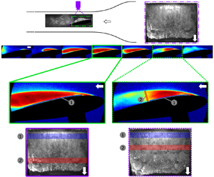
Type (ii) cavities appear for $7.6 > \sigma _{0}/2\alpha > 6.1$ with $0.4 < L_C/C < 0.6$. They are characterized as exhibiting shedding due to cavity pinch-off resulting from liquid re-entrant flow and bubbly shock waves with no obvious preference for either flow front. Figure 11 illustrates a typical shedding cycle of a type (ii) cavity from top-view high-speed video snapshots. During the growth cycle shown in figure 11(a–c), a flow front (yellow arrow) near the leading edge of the hydrofoil is clearly seen. As the cavity reaches a critical length ($L_c$), another flow front travelling towards the leading edge (shown in red arrow) causes the cavity to pinch-off. As observed for type (i) cavities, it was not possible to identify the flow feature that causes shedding from high-speed videos. However, from time-resolved X-ray densitometry observations it was possible to identify both liquid re-entrant flow and bubbly shock-induced cavity pinch-off.

Figure 11. Images of a type (ii) partial cavity at $\sigma _0/2 \alpha = 7.5$. Yellow and red arrows highlight the re-entrant liquid flow and a secondary flow front, respectively. The arrows highlight the flow fronts that lead to cavity pinch-off.

Figure 12 shows time-resolved void fraction flows of a type (ii) cavity shedding cycle caused by a re-entrant liquid flow. The shedding cycle begins with cavity growth as shown in figure 12(a–d). While the cavity grows, liquid accumulates underneath the cavity as shown in figure 12(b,c). This liquid flow underneath the cavity travels upstream, as shown in figure 12(d). Cavity pinch-off occurs near the leading edge and cloud shedding follows, as shown in figure 12(e, f). From these void fraction field measurements the flow structure responsible for the shedding is identified as a liquid re-entrant flow, visualized in figure 12(d).

Figure 12. Time series of void fraction fields, $\beta$, from a shedding type (ii) cavity at $\sigma _0/2 \alpha = 7.5$. The images illustrate a shedding cycle where re-entrant liquid flow causes cavity pinch-off. The location of the two surface pressure transducers are illustrated by the circles. (See supplementary movie 2.)

Bubbly shock driven cavity shedding cycle for a type (ii) cavity is depicted in figure 13. The cycles begins with cavity growth and subsequent attainment of maximum length, as shown in figure 13(a–c). Upon attaining maximum length, the cavity begins to collapse from the rear, and a void fraction discontinuity that represents a bubbly shock is seen in figure 13(d). The bubbly shock waves are characterized by the abrupt change in void fraction ($\beta$) values in a direction tangential to the suction-side surface of the hydrofoil, highlighted in figure 13(d). This bubbly shock wave causes the cavity to pinch-off and shed, as shown in figure 13(e, f).

Figure 13. Time series of void fraction fields, $\beta$, from a cavity for type (ii) at $\sigma _0/2 \alpha = 7.5$. The images illustrate a shedding cycle where the propagation of a bubbly shock front causes cavity pinch-off. The location of the two surface pressure transducers are illustrated by the circles. (See supplementary movie 2.)

Figure 14(a,b) shows the unsteady pressure ${\rm d}p_1$ observed in shedding cycles discussed in figures 12 and 13. For the re-entrant flow driven shedding cycle (figure 14a), ${\rm d}p_1$ reduces from (1) to (2) as the cavity begins to fill with vapour. As the cavity continues to grow and the re-entrant flow develops, ${\rm d}p_1$ does not register an increase in pressure between (2) and (4). From figure 12(d) it is seen that at this instance, when a layer of liquid covers ${\rm d}p_1$, no appreciable increase in pressure is registered by ${\rm d}p_1$. Instead, ${\rm d}p_1$ increases as the re-entrant liquid flow causes cavity pinch-off between figure 14(a)(4,5). This lack of pressure rise is important evidence that the observed flow structure is a liquid re-entrant flow and not a bubbly shock wave. A bubbly shock wave driven shedding cycle is shown in figure 13. When cavity growth begins, the pressure reduces from figure 14(b) (1) to (3), with a peak between (2) and (3). It is not clear what causes this peak, but it is likely due to the shed cloud collapse between (2) and (3), as shown in figure 13(b,c). The cavity collapse begins at (d) and the bubbly shock crosses ${\rm d}p_1$ between (d) and (e), as seen in figure 13(d,e). Passage of the bubbly shock over ${\rm d}p_1$ registers a pressure rise that is annotated in figure 14(b). This pressure rise is between 3–5 kPa depending on the shedding cycle.

Figure 14. The surface pressures ${\rm d}p_1$ for a shedding cycle of a type (ii) cavity at $\sigma _0/2\alpha = 7.5$) with (a) re-entrant liquid flow shedding shown in figure 12 and (b) shock wave driven shedding shown in figure 13.

6. Cavity with shedding caused by bubbly shocks: type (iii)

Type (iii) cavities appear for $6.1 > \sigma _{0}/2\alpha > 5.1$ with $0.6 < L_C/C < 0.85$. Cavity pinch-off is mostly caused by bubbly shock waves with re-entrant flows causing occasional cavity pinch-off. Figure 15 shows a time series of shedding observed for type (iii) cavity at $\sigma _{0}/2\alpha = 5.4$. The cycle begins with the cavity growth near the leading edge, as shown in figure 15(a). Upon attaining a length of about $0.4 C$, a flow structure originates at the closure region of the growing cavity similar to the flow front seen in the closure region of type (i) and (ii) cavities (orange arrows in figure 15b,c). When the cavity attains its maximum length in a given cycle, another feature originates at the closure (red arrows in 15d,e). This structure propagates upstream, significantly faster than the previous structure, causing the cavity to be pinched-off from the leading edge, as shown in figure 15(e–g).

Figure 15. Images of a partial cavity for type (iii) at $\sigma _0/2 \alpha = 5.4$ showing a representative type (iii) cavity. Two flow fronts are observed, with orange and red arrows highlighting each flow front. The flow front highlighted by orange arrows remains trapped underneath the cavity and the red arrow flow front ultimately leads to cavity pinch-off.

Figure 16 shows an X-ray densitometry based void fraction flow field for a type (iii) cavity experiencing bubbly shock-induced shedding. The cycle begins by cavity growth as shown in figure 16(a). The cavity continues to grow and attains a maximum length that extends beyond the X-ray field of view, as seen in figure 16(b–d). During this growth process, liquid accumulates underneath the cavity, with the liquid flow being thicker near cavity closure, as seen in figure 16(b–d). Figure 16(d) also shows a liquid re-entrant flow front near the cavity attachment point. This flow front is almost stationary and unable to cause cavity pinch-off. A bubbly shock causes the cavity to collapse near the cavity closure, travelling past the liquid re-entrant flow to cause pinch-off from the leading edge, as shown in figure 16(e–i).

Figure 16. Time series of void fraction fields, $\beta$, for a type (iii) cavity at $\sigma _0/2 \alpha = 5.4$. The images illustrate a shedding cycle where the propagation of a shock front causes cavity pinch-off. The location of the two surface pressure transducers are illustrated by the circles. From (4) to (7), the trapped re-entrant flow front is unable to cause pinch-off; (5)–(7) shows the advancing shock wave moving upstream to cause pinch-off near the leading edge. (See supplementary movie 3.)

Most of the shedding cycles observed for type (iii) cavities were caused by propagating bubbly shock waves (figure 16), with a liquid re-entrant flow co-existing underneath the cavity but unable to cause pinch-off. Despite the bubbly shock dominant shedding occurring for the majority of the shedding cycles, re-entrant liquid occasionally caused cavity pinch-off near the leading edge of the foil. This is quantitatively presented in figure 26, where despite the dominance of shock waves, re-entrant flow still causes pinch-off. One such cycle where re-entrant flow causes pinch-off is shown in figure 17. Figure 17(a,b) shows the growth and the formation of the liquid re-entrant flow. As the cavity continues to grow, liquid accumulates at the cavity closure due to flow turning and propagates upstream, as shown in figure 17(c,d). This liquid re-entrant flow caused the cavity to pinch-off, as seen in figure 17(e), and the pinch-off occurred while the cavity was still growing. The maximum cavity length for the re-entrant flow caused shedding was shorter than the maximum cavity length seen in bubbly shock caused shedding, and the residual cavity subsequently grows.

Figure 17. Time series of void fraction fields, $\beta$, from a type (iii) cavity at $\sigma _0/2 \alpha = 5.4$. The images illustrate a shedding cycle where re-entrant liquid flow causes cavity pinch-off. The location of the two surface pressure transducers are illustrated by the circles. Despite the dominance of bubbly shock waves as a cavity pinch-off mechanism, the re-entrant liquid flow is sometimes observed to produce cavity pinch-off. (See supplementary movie 3.)

The corresponding unsteady pressure values, ${\rm d}p_1$ and ${\rm d}p_2$ for the shedding cycle depicted in figure 16, are shown in figure 18. During the cavity growth phase, vapour covers the surface of ${\rm d}p_1$ and ${\rm d}p_2$, and a pressure drop is recorded as shown in figure 18(a)(1,2) and (b)(2,3), respectively. Passage of the liquid re-entrant flow over ${\rm d}p_1$ and ${\rm d}p_2$ does not register a substantial pressure rise, as seen in figure 18(a)(3–7) and 18(b)(3–5). A pressure rise due to the passage of the bubbly shock over ${\rm d}p_2$ is seen between 18(b)(5,6) and over ${\rm d}p_1$ in figure 18(a)(7,8). As the cavity pinches off from the leading edge, a large spike in pressure is registered at ${\rm d}p_1$ as the transducer gets exposed to ambient pressure.

Figure 18. The surface pressures ${\rm d}p_1$ (a) and ${\rm d}p_2$ (b) for a shedding cycle of a type (iii) cavity at $\sigma _0/2\alpha = 5.4$ depicted in figure 16. From (4) to (7) the trapped re-entrant flow front does not significantly affect the unsteady surface pressure at ${\rm d}p_1$. A 14.6 kPa pressure rise due to the shock wave front passing over ${\rm d}p_1$ is highlighted between (7)–(8) in (a). Similarly, a 5.9 kPa pressure rise over ${\rm d}p_2$ is highlighted between (5)–(6) in (b).

7. Cavity with dynamics influenced by trailing edge cavitation: type (iv)

Type (iv) cavities appear for $\sigma _{0}/2\alpha < 5.1$ with $L_C/C > 0.85$. Cavity shedding is caused mostly by bubbly shocks, but the influence of trailing edge cavitation is now present. Figure 19 shows snapshots in the form of a time series, depicting shedding observed for a type (iv) cavity at $\sigma _{0}/2\alpha = 4.1$. Here, there is significant cavitation near the trailing edge that interacts with the main cavity forming on the suction side. The rotation of the shed trailing edge cavitation cloud is opposite signed compared with the rotation of the shed cloud from the main cavity over the hydrofoil as seen in Figure 1. Figure 19 shows a type (iv) shedding cycle synchronous with acoustic pressure measurements $p_a$, where $p_a$ is the signal detected by a hydrophone mounted in a liquid pocket located on the top of the tunnel wall 0.25 $C$ away from the trailing edge of the hydrofoil. As the main cavity attains maximum length, the shed cloud from the previous shedding cycle collapses near the trailing edge, as shown in figure 19(a)(3). This collapse causes a pressure pulse that is recorded as a 12 kPa impulse by the hydrophone. After this pressure pulse, the suction-side cavity begins to collapse between (4)–(6), as seen in top-view snapshots in figure 19(c). This illustrates how the collapse of the convecting vapour cloud initiates the following cavity collapse process for a type (iv) cavity.

Figure 19. A time series of high-speed images for type (iv) at $\sigma _0/2 \alpha = 4.1$ that highlights the collapse of a shed vapour cloud downstream of the hydrofoil that then initiates the collapse of the subsequent attached cavity. The hydrophone signal (a) records the acoustic pressure, $p_a$, that is correlated with the images before and after cloud collapse. The corresponding side-view (b) and top-view (c) images show the cloud collapse process. (See supplementary movie 6.)

The void fraction time series depicting shedding dynamics of a type (iv) cavity is shown in figure 20. The cycle begins with cavity growth from the leading edge of the hydrofoil as seen in figure 20(a,b). As the cavity grows, liquid re-entrant flow begins to develop at the cavity closure, as seen in figure 20(c,d), and it travels upstream as seen in figure 20(e–g). However, the cavity collapse is caused by a bubbly shock propagating toward the leading edge, as seen in figure 20(e–h), followed by pinch-off as shown in figure 20(i). The shedding mechanisms observed for type (iv) cavities are similar to type (iii), and both the re-entrant flow and bubbly shock waves are present. Cavity pinch-off was dominated by the propagation of bubbly shock waves and rarely by liquid re-entrant flow. As seen in type (iii) cavities, re-entrant flow can occasionally lead to cavity pinch-off, as shown in figure 21. The re-entrant flow is seen to approach the leading edge from (c)–(e) and cut off the cavity near the leading edge at ( f). The residual cavity then grows and a normal shedding cycle resumes.

Figure 20. Time series of void fraction fields, $\beta$, for a type (iv) cavity at $\sigma _0/2 \alpha = 4.1$. The location of the two surface pressure transducers are illustrated by the circles. A bubbly shock causes the cavity pinch-off, although re-entrant liquid flow can also be observed. (See supplementary movie 4.)

Figure 21. Time series of void fraction fields, $\beta$, from a type (iv) shedding cavity at $\sigma _0/2 \alpha = 4.1$, where liquid re-entrant flow causes cavity pinch-off near the leading edge. (See supplementary movie 4.)

To visualize cavitation near the trailing edge the field of view of the densitometry system was moved downstream. A time series of instantaneous void fraction measurements for type (iv) cavitation near the trailing edge is shown in figure 22. The cycle starts with the pinch-off of the main cavity on the surface of the hydrofoil caused by a bubbly shock, as shown in figure 22(a). As the bubbly shock travels upstream, vapour is shed from the interface and this shed vapour cloud is seen near the trailing edge in figure 22(b,c). Meanwhile, cavitation occurs at the trailing edge on the suction side and begins to interact with the shed cloud in figure 22(c,d) forming lobe 1. As the shed vapour from the main cavity moves downstream, it interacts with lobe 1, causing formation of lobe 2 in figure 22( f,g). Lobe 2 interacts with lobe 1 in figure 22(g–i) and a cloud is shed from the trailing edge in figure 22( j). The presence of a long and thick cavity on the hydrofoil, as observed in type (iv), is similar to open cavities observed in wakes, as discussed in Wu et al. (Reference Wu, Deijlen, Bhatt, Ganesh and Ceccio2021). The thick cavity shed from the suction side and the trailing edge are counter-rotating, resembling spanwise vortices in the near-wake region of a bluff body. They interact in a manner similar to the two counter-rotating spanwise vortices observed in the cavitating wakes of two-dimensional bluff bodies (Wu et al. Reference Wu, Deijlen, Bhatt, Ganesh and Ceccio2021).

Figure 22. Time series of void fraction fields, $\beta$, for a type (iv) at $\sigma _0/2 \alpha = 4.1$. The field of view is moved downstream to show the trailing edge. The location of the aft surface pressure transducers is illustrated by the circle. The cavity shed from the suction side and the trailing edge cavity interact, and this interaction is similar to that between two counter-rotating regions of cavitating flow observed in wakes of bluff objects, as discussed by Wu et al. (Reference Wu, Deijlen, Bhatt, Ganesh and Ceccio2021). (See supplementary movie 5.)

8. Re-entrant flow and bubbly shock properties

Re-entrant flow thickness was estimated using high-speed images. When re-entrant liquid flows were observed, the thickness of the re-entrant flow, $t_J$, at 85 % of $L_C$ is typically 0.3 to 3.2 mm or roughly 5 % to 15 % of the maximum cavity thickness, $t_C$, as shown in figure 23. Observed re-entrant flow thickness in the present study is less than half the typical value reported by Callenaere et al. (Reference Callenaere, Franc, Michel and Riondet2001) for a cloud shedding cavity formed behind a backward facing step (15 % to 35 % of the maximum cavity thickness). The re-entrant flow convects upstream from the closure region of the cavity and can cause the cavity to separate when it impinges near the hydrofoil leading edge. The average re-entrant flow speed estimated from void fraction fields is between 3 and 6 m s$^{-1}$, or roughly 41–75 % of the free-stream speed. This range is consistent with the observations reported by Callenaere et al. (Reference Callenaere, Franc, Michel and Riondet2001).

Figure 23. Maximum cavity thickness, $t_C/C$ ($\blacklozenge$), and re-entrant flow thickness, $t_J/t_C$ (red triangle right), varying with $\sigma _0/2\alpha$.

For cavities with bubbly shock waves, we can measure the shock speed directly from the examination of $s-t$ diagrams of near-surface void fraction, as discussed by Ganesh et al. (Reference Ganesh, Makiharju and Ceccio2016) and Bhatt et al. (Reference Bhatt, Ganesh and Ceccio2021). The $s-t$ diagrams trace the change in void fraction values along the tangential curve ‘s’ on the suction side of the hydrofoil, as shown in figure 24, with time. In addition, the shock speed can be independently estimated using conservation of mass and momentum across a normal shock interface. Assuming negligible heat transfer and neglecting bubble dynamics, the expression for shock propagation speed, $u_S$, can be obtained by using (Brennen Reference Brennen2005),

(8.1)\begin{equation} u_S^2 = \frac{ (p_2-p_1) }{\rho_L} \left[\frac{(1-\beta_2)}{(1-\beta_1)(\beta_1-\beta_2)}\right], \end{equation}

where $\beta _1$ and $\beta _2$ are the void fraction values upstream and downstream of the front, and $p_2-p_1$ is the pressure rise across the front. The void fraction is measured from the X-ray measurements, and the pressure rise is determined from the unsteady surface pressure measurements as the front passes over the transducer. The direct measurement of $u_S$ is made in the laboratory frame using the $s-t$ diagram generated along the curve parallel to the surface of the hydrofoil, as shown in figure 24. Figure 25 presents the directly measured and the computed shock speed normalized by the upstream flow speed, $u_S/u_0$. The speed computed using (8.1) is consistent with the speed that was directly measured. This implies that the jump conditions adequately captures the mass and momentum conservation across the shock front, and that velocity of the bubbly mixture within the cavity is much slower (e.g. closer to zero speed) than the shock speed as it convects upstream. The shock speed peaks for type (iv) cavities, which also are dominated by shock-induced shedding processes.

Figure 24. Schematic depicting the tangential direction ($s$) and normal direction ($n$) to the surface of the hydrofoil. The $s-t$ diagrams are made using the curve (red dashed line) and $u_S$ is measured directly.

Figure 25. The shock speed $u_S/u_0$ for varying of $\sigma _0/2\alpha$. The speed was directly measured in the laboratory frame ($\blacksquare$) and computed using (8.1) (red diamond) for hydrofoil at $\alpha = 10^{\circ }$.

9. Probability that re-entrant flows or bubbly shock waves will lead to cavity pinch-off

The results presented above illustrate that cavity pinch-off can be caused by both re-entrant flows and bubbly shocks. With changing $\sigma _0/2 \alpha$, we see that the likelihood of pinch-off caused by either cavity shedding mechanism changes. In this section the probability of cavity pinch-off caused by re-entrant flows and bubbly shock waves is estimated. We define the event probability as the probability of cavity shedding caused by a particular mechanism as determined from time-resolved void fraction measurements. The probability definitions are shown in (9.1) and (9.2), where $N_R$, $N_S$ are the number of re-entrant flow driven shedding cycles and shock wave driven shedding cycles, respectively, for $N$ total cycles,

(9.1)$$\begin{gather} P_R = \dfrac{N_R}{N}, \end{gather}$$

(9.2)$$\begin{gather}P_S = \dfrac{N_S}{N}. \end{gather}$$

Figure 26 shows the probability of liquid re-entrant flow and bubbly shock waves to cause cavity pinch-off for a given $\sigma _0/2 \alpha$ at $\alpha = 10^{\circ }$. As $\sigma _0/2 \alpha$ is reduced, the likelihood of pinch-off caused by bubbly shock increases and the likelihood of pinch-off caused by re-entrant flows decreases. The dominance of each flow front in different cavity shedding regimes can also be seen as $\sigma _0/2 \alpha$ is reduced. We next consider the relationship between Mach number within the partial cavity and the likelihood of bubbly shock formation.

Figure 26. Event probability plot showing the probability of re-entrant flow causing cavity pinch-off, $P_R$ ($\bigcirc$), along with bubbly shock waves causing pinch-off, $P_S$ ($\square$), as a function of $\sigma _0/2\alpha$. For longer type (iii) and type (iv) cavities, shock waves are the dominant mechanism of shedding, but re-entrant liquid jets can still cause cavity detachment.

Previous studies such as Ganesh et al. (Reference Ganesh, Makiharju and Ceccio2016), Budich et al. (Reference Budich, Schmidt and Adams2018), Bhatt & Mahesh (Reference Bhatt and Mahesh2020), Wu et al. (Reference Wu, Deijlen, Bhatt, Ganesh and Ceccio2021) and Bhatt et al. (Reference Bhatt, Ganesh and Ceccio2021) have reported on the effect of mixture compressibility on the dynamics of high void fraction cavitating flows. At void fraction values $\beta > 0.1$, the speed of sound of the bubbly mixtures rapidly reduces and reaches a minimum around $\beta \approx 0.5$ (Brennen Reference Brennen2005). The sound speed of a cavitating bubbly mixture can be on the same order or slower than the speed of the surrounding liquid flow, making it locally supersonic and susceptible to the occurrence of bubbly shocks. By estimating the local speed of sound of the bubbly mixture within the separated region of the partial cavity, a Mach number based on the relevant velocity scales can be defined. The relationship between the likelihood of a given shedding mechanism and the estimated Mach number can then be sought.

The local speed of sound can be estimated by using a simplified expression for a homogeneous vapour–liquid mixture (Brennen Reference Brennen2005). Bhatt et al. (Reference Bhatt, Ganesh and Ceccio2021) demonstrated that the simplified speed of sound expression for a bubbly mixture is able to predict the onset of bubbly shock waves in shedding partial cavities behind a backward facing step. The general expression for the mixture sound speed is based on the assumption that the homogeneously dispersed vapour phase (subscript $V$) and the carrier liquid (subscript $L$) have no relative motion with negligible surface tension effects. Here, $\epsilon _L$ ($\epsilon _V$) is the fraction of the liquid (vapour) phase in thermodynamic equilibrium with the vapour (liquid) phase. The general expression for the mixture speed of sound, $c$, is given by

(9.3)\begin{equation} \frac{1}{\rho_m {c}^2}=\frac{\beta}{p}[ (1-\epsilon_V) f_V+ \epsilon_V g_V] +\frac{1-\beta}{{p}^{1+\eta}}\epsilon_L g^* p_{cr}^{\eta}, \end{equation}

where $\beta$ is the mixture void fraction, $\rho _m = \beta \rho _V + (1-\beta )\rho _L$ is the mixture density and $p$ is the mixture pressure. For water, $g^* = 1.67$, $\eta = 0.73$, $g_V = 0.91$, $f_V = 0.73$ and $p_{cr} = 22.06$ MPa (Brennen Reference Brennen2005). For a general two component system with no inherent assumptions, $g^*$, $\eta$, $g_V$ and $f_V$ are thermodynamic functions encapsulating latent heat and temperature. We can make two bounding assumptions for heat transfer during phase change to develop the ‘homogeneous equilibrium model’ and the ‘homogeneous frozen model.’ The equilibrium model assumes instantaneous heat transfer between phases with $\epsilon _V=\epsilon _L = 0$, while the frozen model assumes zero heat transfer between phases with $\epsilon _V=\epsilon _L = 1$. The sound speed of a real two-phase mixture may lie somewhere between these bounds (Budich et al. Reference Budich, Schmidt and Adams2018).

Bhatt et al. (Reference Bhatt, Ganesh and Ceccio2021) studied the validity of sound speed expressions based on the homogeneous frozen model and the homogeneous equilibrium model in predicting the experimental onset of bubbly shocks. They observed that the Mach number defined based on the velocity at the point of separation of the step and sound speed based on the homogeneous frozen model exhibited a subsonic to supersonic transition that coincided with the experimental observations of bubbly shocks. This result was contrasted with the Mach number based on the same velocity scale and sound speed based on the homogeneous equilibrium model, where the predicted Mach number was two orders of magnitude higher and, hence, always supersonic. Based on these findings, we will use the frozen model to estimate the local speed of sound (and Mach number) in the bubbly mixture within the cavity of the NACA0015 hydrofoil.

To evaluate the minimum sound speed based on (9.3), we need to determine the mixture pressure when the cavity is filled with vapour. The average static pressure within the cavity, $p_c$, was measured at the location depicted in figure 4(a), and this value represents the static pressure averaged over the entire shedding cycle. This includes conditions when the cavity mixture covers the pressure port as well as when the liquid flow is present over the measurement location. To determine the cavity pressure when the transducer is covered with vapour, we combine the average pressure value with time-synchronized surface pressure data from the unsteady pressure transducer, ${\rm d}p_1$, recorded at the same downstream location. As shown in the previous section, the dynamic pressure signal is correlated with various steps of the shedding cycle. The pressure change registered by ${\rm d}p_1$ can be subtracted from the mean pressure within the cavity to estimate static pressure at the time of shock propagation. This pressure is defined as $p_S$, such that $p_S=p_c-p^{*}$, where $p^{*}$ is the pressure rise recorded by ${\rm d}p_1$ immediately after passage of the bubbly shock. Based on these static pressures, we can define a pressure coefficient, $C_{p}$ as

(9.4)\begin{equation} C_{p}=\frac{p-p_0}{\frac{1}{2} \rho u^2_0}, \end{equation}

where $p$ is a pressure of interest ($p_c$, $p_S$). The respective pressure coefficients ($C_{p_c}$, $C_{p_S}$) are shown in figure 27.

Figure 27. The pressure coefficients $-C_{p_C}$ ($\blacksquare$) and $-C_{p_S}$ (red triangle right) varying with $\sigma _0/2\alpha$ for the foil at $\alpha =10^{\circ }$.

We can determine the mixture sound speed, $c$, based on $p_S$ and corresponding void fraction measurement. The Mach number $M_0$ is defined based on ‘$c$’ and inflow velocity $u_0$ as

(9.5)\begin{equation} M_0 = \dfrac{u_0}{c}. \end{equation}

For every instantaneous void fraction flow field, a spatially varying Mach number field based on the cavity pressure $p_S$ can be estimated. From this field we can then estimate the maximum cavity Mach number, $M_{0P}$, that corresponds to the condition of maximum cavity void fraction and minimum static pressure. Figure 28 shows the variation of $M_{0P}$ with $\sigma _0/2\alpha$ as a box plot. The boxes represent the median, the 75th and 25th percentiles. The whiskers represent the maximum and minimum values. The data in figure 28 reveals that the onset of bubbly shock waves coincides with the transition of the peak value $M_{0P}$ from subsonic to supersonic. For type (iii) and (iv) cavities, $M_{0P} >1$, both the upper and lower whiskers lie above unity. For type (ii) cavities, it is likely that $M_{0P} > 1$ for many cycles, and for type (i) cavities, there are conditions where the local Mach number does not reach unity. The median value of $M_{0P}$ increases with decreasing $\sigma _0/2\alpha$ in tandem with the increasing likelihood of shock formation, as shown in figure 26.

Figure 28. Box plot depicting variation of the peak value of $M_{0P}$ that occurs over one shedding cycle with decreasing $\sigma _0/2\alpha$ across the different cavitation regimes. The boxes represent the median, the 75th and 25th percentiles. The whiskers represent the maximum and minimum values.

We can also define a Mach number, $M_S$, using the local sound speed derived from the pressure within the cavity at the time of shock propagation, $c$, and shock speed, $u_S$, presented in figure 25 as

(9.6)\begin{equation} M_S = \dfrac{u_S}{c}, \end{equation}

here $M_S$ allows us to compare the shock propagation speed with our estimate of the mixture sound speed at the time of shock formation and propagation. Figure 29 presents $M_S$ varying with $\sigma _0/2\alpha$ as a box plot. The shock speed $u_S$ can be determined directly from the $s-t$ diagrams and from one-dimensional jump relations based on pressure measurements from ${\rm d}p_1$. The data from the direct measurement of the shock speed and from those inferred from the jump conditions are both shown, where $M_{SD}$ is determined from the directly measured shock speed and $M_{SJ}$ were computed using the jump condition, (8.1). The onset of type (ii) cavities have $M_S < 1$, but as $\sigma _0/2\alpha$ is reduced, the Mach number increases, crossing the $M_{S} = 1$ boundary.

Figure 29. Box plot depicting variation of the peak value of $M_S$ that occurs over multiple shedding cycles with decreasing $\sigma _0/2\alpha$. The boxes represent the median, the 75th and 25th percentiles, and the whiskers represent the maximum and minimum values. The data from the direct measurement of the shock speed and from those inferred from the jump conditions are both shown, where (a) $M_{SD}$ were determined from the directly measured shock speed, and (b) $M_{SJ}$ were computed using the jump condition, (8.1).

The onset of supersonic cavity conditions correlates with the increased probability of shock wave formation. Figure 30 shows a composite plot with the event probability of liquid re-entrant flow and bubbly shock waves along with the mean and standard deviation of $M_0$, $M_{SD}$ and $M_{SJ}$. The trend in increasing probability of shock formation with increasing average Mach number is clearly observed. The Mach number defined with the local shock speed is lower than that defined with the inlet velocity, since the shock speed is often (but not always) lower than the free-stream speed. Here, $M_S$ transitions from subsonic to supersonic near the value of $\sigma _0/2\alpha$ where there is equal probability of re-entrant flow or bubbly shock-induced shedding. The observation that the onset of shock formation corresponds to the transition from subsonic to supersonic conditions within the cavity is consistent with the observations of Bhatt et al. (Reference Bhatt, Ganesh and Ceccio2021).

Figure 30. Variation of mean and standard deviation of $M_{0P}$ ($\rhd$), $M_{SD}$ ($\blacksquare$), and $M_{SJ}$ (red diamond) with $\sigma _0/2\alpha$. The event probability data $P(R)$ ($\bigcirc$) and $P(S)$ ($\square$) are also shown. The horizontal dashed line demarcates where $M = 1$.