Hostname: page-component-745bb68f8f-5r2nc Total loading time: 0 Render date: 2025-01-09T19:03:26.745Z Has data issue: false hasContentIssue false

On the origin of counter-gradient transport in turbulent scalar flux: physics interpretation and adjoint data assimilation

Published online by Cambridge University Press:  19 November 2024
Sen Li
Affiliation:
Key Laboratory of Education Ministry for Power Machinery and Engineering, School of Mechanical Engineering, Shanghai Jiao Tong University, 800 Dongchuan Road, Shanghai 200240, PR China
Wenwu Zhou
Affiliation:
Key Laboratory of Education Ministry for Power Machinery and Engineering, School of Mechanical Engineering, Shanghai Jiao Tong University, 800 Dongchuan Road, Shanghai 200240, PR China
Hyung Jin Sung
Affiliation:
Department of Mechanical Engineering, KAIST, 291 Daehak-ro, Yuseong-gu, Daejeon 34141, Korea
Yingzheng Liu*
Affiliation:
Key Laboratory of Education Ministry for Power Machinery and Engineering, School of Mechanical Engineering, Shanghai Jiao Tong University, 800 Dongchuan Road, Shanghai 200240, PR China
*
Email address for correspondence: [email protected]

Abstract

The present study offers a twofold contribution on counter-gradient transport (CGT) of turbulent scalar flux. First, by examining turbulent scalar mixing through synchronized particle image velocimetry and planar laser-induced fluorescence on an inclined jet in cross-flow, we clarify the previously unexplained phenomenon of CGT, revealing key flow structures, their spatial distribution and modelling implications. Statistical analysis identifies two distinct CGT regions: local cross-gradient transport in the windward shear layer and non-local effects near the wall after injection. These behaviours are driven by specific flow structures, namely Kelvin–Helmholtz vortices (local) and wake vortices (non-local), suggesting that scalar flux can be decomposed into a gradient-type term for gradient diffusion and a term for large-eddy stirring. Second, we propose a new approach for reconstruction of turbulent mean flow and scalar fields using continuous adjoint data assimilation (DA). By rectifying model-form errors through anisotropic correction under observational constraints, our DA model minimizes discrepancies between experimental measurements and numerical predictions. As expected, the introduced forcing term effectively identifies regions where traditional models fall short, particularly in the jet centreline and near-wall regions, thereby enhancing the accuracy of the mean scalar field. These enhancements occur not only within the observation region but also in unseen regions, underscoring present DA approach's reliability and practicality for reproducing mean flow behaviours from limited data. These findings lay a solid foundation for adjoint-based model-consistent data-driven methods, offering promising potential for accurately predicting complex flow scenarios like film cooling.

Type
JFM Papers
Copyright
© The Author(s), 2024. Published by Cambridge University Press

1. Introduction

Scalar transport problems, which characterize mass and heat transfer behaviours in fluid dynamics, are prevalent in various shear-dominated applications like premixed turbulent flames, pollutant in plumes and film cooling in aeroengines. One of the most prominent features of such transport is the presence of large-scale coherent structures in the mixing layer (Li, Balaras & Wallace Reference Li, Balaras and Wallace2010). These structures induce turbulent scalar flux that flows along the direction opposite to the mean scalar profile gradient, giving rise to counter-gradient transport in mixing; such a fact certainly diverges from the conventional understanding in first-order turbulent closure (Xiao & Cinnella Reference Xiao and Cinnella2019) presuming that turbulent diffusion typically follows the scalar gradient. However, despite numerous observations of counter-gradient transport in turbulent scalar flux (Veynante et al. Reference Veynante, Trouvé, Bray and Mantel1997; Mahesh Reference Mahesh2013), a notable research gap persists in understanding the underlying cause-and-effect mechanism and the corresponding implications for modelling. Accordingly, it is highly desirable to addressing the challenging issues in Reynolds-averaged Navier–Stokes (RANS)-based models.

Both experimental data (Su & Mungal Reference Su and Mungal2004) and theoretical analyses (Muppidi & Mahesh Reference Muppidi and Mahesh2008) have highlighted the existence of counter-gradient transport, which contributes decisively to poor mean scalar field predictions. The observation of counter-gradient transport in laboratory settings was initially documented by Komori et al. (Reference Komori, Ueda, Gino and Mizushina1983) in a thermally stratified open-channel water flow. Subsequently, Veynante et al. (Reference Veynante, Trouvé, Bray and Mantel1997), Salewski, Stankovic & Fuchs (Reference Salewski, Stankovic and Fuchs2008) and Milani, Ling & Eaton (Reference Milani, Ling and Eaton2020) reported instances of counter-gradient heat or mass transfer in various applications. Among all scenarios, the jet-in-cross-flow (JICF) has received widespread attention. Su & Mungal (Reference Su and Mungal2004) scrutinized the time-averaged turbulence quantities through simultaneous measurements of scalar and velocity field and were the first to identify the region of counter-gradient transport of turbulent scalar flux in JICF. Veynante et al. (Reference Veynante, Trouvé, Bray and Mantel1997) endeavoured to measure the co-spectra of instantaneous momentum and scalar fluxes; however, significant scattering was encountered in the circular JICF, posing challenges in precisely identifying the scale motions contributing to counter-gradient transport. Milani et al. (Reference Milani, Ling and Eaton2020) identified two types of counter-gradient transport (CGT) in JICF, occurring within the jet shear layer and near wall region, consistent with observations by Muppidi & Mahesh (Reference Muppidi and Mahesh2008). They demonstrated that in the jet shear layer, cross-gradient effects play a significant role in counter-gradient heat transfer, whereas in the near-wall region, non-local contributions predominate. Nevertheless, the underlying mechanism driving these behaviours remains unclear.

Parallelly, many efforts have been directed towards enhancing the predictive capabilities of RANS models for scalar mixing, including adjustments to isotropic assumptions (Bergeles, Gosman & Launder Reference Bergeles, Gosman and Launder1978; Lakehal, Theodoridis & Rodi Reference Lakehal, Theodoridis and Rodi2001; Liu, Zhu & Bai Reference Liu, Zhu and Bai2008, Reference Liu, Zhu and Bai2011; Ling, Rossi & Eaton Reference Ling, Rossi and Eaton2015; Zhang et al. Reference Zhang, Mao, Su and Yuan2022b) or the implementation of anisotropic modifications (Azzi & Lakehal Reference Azzi and Lakehal2001; Li et al. Reference Li, Qin, Ren and Jiang2014; Milani et al. Reference Milani, Ling and Eaton2020; Weatheritt et al. Reference Weatheritt, Zhao, Sandberg, Mizukami and Tanimoto2020). Bergeles et al. (Reference Bergeles, Gosman and Launder1978) pioneered the work by adjusting eddy viscosity through a correction factor based on wall-normal distance. Lakehal et al. (Reference Lakehal, Theodoridis and Rodi2001) extended this to include the viscous sublayer. Despite improvements in spreading behaviour, scalar mixing was still overestimated. Azzi & Lakehal (Reference Azzi and Lakehal2001) introduced an explicit algebraic stress model to address near-wall anisotropy, yet still struggled to capture actual spreading. This again emphasizes taking turbulent scalar flux into consideration is essentially important for accurate scalar diffusion. One avenue of exploration was to analyse the turbulent Prandtl number ($P{r_t}$) and devise a case-dependent correction model, showing improved predictions over the gradient diffusion hypothesis (GDH) with uniform $P{r_t}$ distribution (Liu et al. Reference Liu, Zhu and Bai2008). Further enhancements were made by using scalar gradient as a model input (Liu et al. Reference Liu, Zhu and Bai2011) and adapting the model near solid walls to address disparities in behaviour between Reynolds stress and turbulent scalar flux (Ling et al. Reference Ling, Rossi and Eaton2015). Subsequently, the limitations of GDH were successfully surpassed by recent artificial intelligence related efforts. Milani et al. (Reference Milani, Ling and Eaton2020) employed a tensor basis neural network to consider the anisotropic diffusion on the scalar flux transport, while Weatheritt et al. (Reference Weatheritt, Zhao, Sandberg, Mizukami and Tanimoto2020) used gene-expression programming to enhance the accuracy of the turbulent scalar flux ($\overline {{u^{\prime}_i}c^{\prime}} $). These first data-driven endeavours underscore the significance of anisotropic modifications on scalar predictions, as several challenges are often overlooked. First, turbulence modelling for momentum equations alters mean velocity, and thus affects scalar advection. Second, turbulent mixing models depend explicitly on momentum-derived quantities such as turbulent eddy viscosity. Third, anisotropic modifications inherently suffer from extreme numerical instability (Milani et al. Reference Milani, Ling and Eaton2020). These complex implications indicate the necessity for careful consideration of scalar mixing in turbulent flow.

Fortunately, data assimilation (DA) has emerged as a promising approach to enhance the representation of Reynolds stress and turbulent scalar flux by integrating measurements and numerical simulations (Heitz, Mémin & Schnörr Reference Heitz, Mémin and Schnörr2010; Duraisamy, Iaccarino & Xiao Reference Duraisamy, Iaccarino and Xiao2019; Brunton, Noack & Koumoutsakos Reference Brunton, Noack and Koumoutsakos2020). The essential aspect of a DA scheme lies in its optimization strategy. For mean flow recovery, two categories of DA strategies are used: parametric (Kato et al. Reference Kato, Yoshizawa, Ueno and Obayashi2015; Li et al. Reference Li, Zhang, Bailey, Hoagg and Martin2017, Reference Li, Hoagg, Martin and Bailey2018) and non-parametric methods (Foures et al. Reference Foures, Dovetta, Sipp and Schmid2014; Brener et al. Reference Brener, Cruz, Thompson and Anjos2021; He, Wang & Liu Reference He, Wang and Liu2021; Hafez, Abd El-Rahman & Khater Reference Hafez, Abd El-Rahman and Khater2022; Li, He & Liu Reference Li, He and Liu2022; Zhang et al. Reference Zhang, Xiao, Luo and He2022a,Reference Zhang, Mao, Su and Yuanb, Reference Zhang, Xiao, Luo and He2023a). Parametric approaches involve adjusting RANS closure coefficients based on flow sensitivity distribution. Techniques such as perturbation-based adaptation (Duraisamy et al. Reference Duraisamy, Iaccarino and Xiao2019) or statistical approaches like the ensemble Kalman filter (EnKF) (Kato et al. Reference Kato, Yoshizawa, Ueno and Obayashi2015) have shown improved mean flow reconstruction. However, their reliance on ensemble-based techniques results in high computational costs, and their reliability is constrained by the structure of turbulence models. Non-parametric methods address these limitations by introducing modifications directly into turbulent transport equations or model terms, such as Reynolds stress or eddy viscosity. Singh & Duraisamy (Reference Singh and Duraisamy2016) introduced a multiplicative correction into the production terms of the turbulent transport equation using the discrete adjoint method, achieving high-fidelity mean flow reconstruction. Efforts to extend the solution space of non-parametric approaches were made by directly perturbing Reynolds stresses through iterative EnKF methods (Zhang et al. Reference Zhang, Xiao, Luo and He2022a, Reference Zhang, Xiao, Luo and He2023a), adjusting the Reynolds force vector (the divergence of the Reynolds stress) using adjoint-based approaches (Foures et al. Reference Foures, Dovetta, Sipp and Schmid2014; Symon et al. Reference Symon, Dovetta, McKeon, Sipp and Schmid2017) or incorporating the eddy viscosity model in high-Reynolds-number flows (He et al. Reference He, Wang and Liu2021; Li, He & Liu Reference Li, He and Liu2022). As mixing is predominantly governed by convection transport and turbulent scalar flux transport, both factors should be taken into full consideration in the DA framework; however, rather few efforts in this strategy have been reported.

The major attention of the present work is placed on predicting the counter-gradient transport of turbulent scalar flux using an improved DA framework for Reynolds stress and turbulent scalar flux. Towards this end, the present paper offers a twofold contribution. First, we employed an inclined JICF under two distinct flow regimes to elucidate the underlying driving mechanism in regions exhibiting counter-gradient transport of turbulent scalar flux. Second, we delve into the reconstruction of turbulent mean flow and scalar field for inclined JICF using continuous adjoint data assimilation. Model-form errors resulting from the Boussinesq approximation and the GDH are rectified through anisotropic correction under the constraint of observational data. The DA model is derived to minimize discrepancies between the particle image velocimetry (PIV)/planar laser induced fluorescence (PLIF) measurements and the numerical predictions, and thus enable determination of the optimal contribution of the Reynolds force vector and turbulent scalar force (the divergence of the turbulent scalar flux). Here, only limited data are used for DA, and other data are reserved for validation. Finally, the velocity reconstruction of the DA model for two scenarios with different velocity ratios has been validated, and the application of the DA approach to correct the scalar field is explored.

2. High-fidelity database and validation

2.1. Generation of high-fidelity database

The observational datasets for DA were obtained through synchronized time-resolved PIV/PLIF measurements. Additionally, delayed detached eddy simulations (DDESs) were conducted to quantitatively benchmark the reconstruction capabilities of the DA procedure. The experiment set-up, depicted in figure 1, involves a water tunnel submerged within a large glass tank. To ensure a stable mainstream flow, a honeycomb and a contraction section were positioned upstream of the 600-mm-long test section, which features a cross-section of 80 mm (width) × 50 mm (height). The free stream turbulence level is roughly 5 %. During the experiments, the cross-flow velocity at the inlet of the test section was maintained at ${U_0} = 0.38\;\textrm{m}\;{\textrm{s}^{ - 1}}$, corresponding to a Reynolds number of 150 000 based on the distance between the leading edge of the test plate and the coolant injection holes. Two different velocity ratios ($VR = {U_j}/{U_0} = 0.4$ and $1.2$, where ${U_j}$ is the mean jet velocity) were examined by adjusting the jet flow rate. These ratios represent both attached and detached flow regimes, resulting in jet Reynolds numbers (based on the tube diameter) of 1200 and 3600, respectively. Both the cross-flow and jet flow Reynolds number falls in the scope of the typical engine condition (Ye et al. Reference Ye, Liu, Zhu and Luo2019). A constant-head tank was employed to maintain a consistent water level, while a jet chamber was used to stabilize the jet before introduction into the mainstream. Multi-plane measurements ($z/D = 0,\;0.3$ and $0.5$) were conducted to comprehend the three-dimensional flow features in JICF. The jet originated from a circular tube with dimensions: diameter ($D$) of 8 mm, length ($L$) of 40 mm, and an inclination angle ($\alpha $) of 30°. This configuration was selected for its representativeness of film cooling applications, highlighting the highly non-uniform and secondary flow characteristics within the hole.

Figure 1. Experimental set-ups for the simultaneous PIV/PLIF measurements.

A continuous 532-nm laser illuminated PIV particles and served as the excitation source for rhodamine solution in PLIF measurements. Synchronized measurements were performed using two high-speed cameras (Dimax HS, PCO) to capture instantaneous velocity and concentration field. The velocity fields were determined using the adaptive cross-correlation PIV algorithm with 32 × 32 pixels interrogation window and 50 % overlap, resulting in a grid spacing of $0.05D$. Rhodamine dye, with a concentration of ${C_0} = \; 0.05\;\textrm{mg}\;{\textrm{L}^{ - 1}}$, was employed as the jet fluid source. To eliminate the excitation source, a long-wave-pass filter (570 nm) was positioned before the camera lens. The sampling frequency was 1000 Hz and PLIF images had a spatial resolution of $0.02D$.

The computational domain mirrors the experimental set-up depicted in figure 1, with the mainstream inlet boundary located $4.0D$ upstream of the jet exit centre. The numerical simulation incorporates the water chamber, consistent with established film cooling practices, to resolve the recirculation occurring inside the hole before encountering the cross-flow (Bodart, Coletti & Eaton Reference Bodart, Coletti and Eaton2013). In figure 2(c), time-averaged velocity profiles extracted at $x/D ={-} 1.5$ in three measurement planes are shown. Notably, the velocity profiles exhibit good agreement, supporting the notion of treating the mainstream inlet velocity as uniformly distributed along the spanwise direction. To replicate the experimental environment in the numerical simulation, the inflow statistics are derived from time-resolved PIV measurements. The spectral synthesizer, originally proposed by Kraichnan (Reference Kraichnan1970) and modified by Smirnov, Shi & Celik (Reference Smirnov, Shi and Celik2001), is employed to impose the desired flow statistics. Since PIV data for the Reynolds stresses out of the $xy$-plane are unavailable, we resemble these stresses based on the distribution from the high-fidelity simulation of a turbulent inclined JICF by Bodart et al. (Reference Bodart, Coletti and Eaton2013) with a mean turbulence intensity of 5 %. These inflow statistics, extracted at $x/D ={-} 1.5$ from PIV measurements, are applied to the DDES with the mainstream inlet boundary located $4.0D$ upstream of the jet exit centre (figure 2b). The cross-flow boundary layer characteristics $1.5D$ upstream of the jet orifice are then verified using the DDES statistics for velocity and Reynolds stress behaviour. Despite some discrepancies in turbulence statistics, the mean velocity agrees well with the experiments, as shown in figure 2(dg). For the Spalart–Allmaras (SA) model, we impose the turbulent mean velocity profile and the actual eddy viscosity determined from PIV, as depicted in figure 2(c). The eddy viscosity ratio is determined by the linear relationship of the Boussinesq hypothesis, as suggested by Weatheritt et al. (Reference Weatheritt, Zhao, Sandberg, Mizukami and Tanimoto2020). At the chamber inflow, velocity and concentration are imposed without any superimposed turbulence. Figure 2(b) depicts the numerical meshes of the JICF configuration. The computational grids are block-structured and locally refined with 100 inflation boundary layers in the region of interest ($- 1.5 < x/D < 5$, $0 < y/D < 2$ and $- 1.5 < z/D < 1.5$) to better resolve the gradients near the shear layer and solid surfaces. The grid resolution ensures that the first cell centre is located at ${y^ + } < 1.5$ for all walls, except for the upper wall where a slip boundary condition is applied. This set-up adequately captures the blockage effect (Li, He & Liu Reference Li, He and Liu2023). An in-house dynamic DDES code (He, Liu & Yavuzkurt Reference He, Liu and Yavuzkurt2017) is employed for the simulation on a refined mesh comprising either 9.1 million ($VR = 0.4$) or 10.3 million ($VR = 1.2$) elements. The time step size, $\Delta t_{DDES}^ + = \Delta {t_{DDES}}{U_0}/D = 0.01$, ensures that the maximum Courant–Friedrichs–Lewy number is always less than 1. A statistically steady state is reached after 100 time units, where $T = D/{U_0}$. Turbulent quantities are then averaged over a period of 200T, which leads to an acceptable level of convergence for this fully non-homogeneous configuration in which no spatial averaging can be employed to accelerate the convergence.

Figure 2. (a) Schematic of the computational domain, (b) computational mesh with every 10 grid nodes displayed, (c) profiles of the streamwise velocity and the eddy viscosity ratio ${v_t}/v$ determined through PIV measurements and (dg) comparison of velocity and turbulence statistics extracted from $x/D ={-} 1.5$.

2.2. Model validation

The mean turbulent flow, as determined by DDES and SA models, was validated against PIV/PLIF measurements in the mid-plane (figures 3 and 4). The scalar transport in SA model employs a straightforward, isotropic GDH, where the turbulent diffusivity is prescribed with a fixed turbulent Schmidt number, denoted as $S{c_t} = 0.85$ (Kays Reference Kays1994). Regarding the $x$-direction velocity, all profiles exhibit favourable agreement between experimental data and DDES results. However, the SA model fails to accurately capture jet spreading and diffusion, leading to noticeable discrepancies. Two significant distinctions between the default SA model and PIV/DDES results are observed from the contours in figure 3(a,c). First, the pattern of the jet core, as indicated by the $x$-direction velocity, varies noticeably. The experimental and DDES results reveal a broader jet core that extends deeper into the mainstream, whereas the default SA model predicts a narrower core squeezed into the upstream region of the jet, leading to increased $y$-direction velocity. Second, the $x$-direction velocity downstream of the injection, simulated using the default SA model, is notably lower compared with the reference data. This discrepancy is particularly pronounced in the velocity profiles in figure 4(ad). There are two local maxima for each velocity ratio, representing the upstream and downstream shear layers, respectively. The SA model consistently underestimates $x$-direction velocity for both shear layers across all velocity ratios. Additionally, it is important to emphasize that the cross-flow incoming boundary layer is thicker than the other two, indicating an overestimation of eddy viscosity in front of the jet. This discrepancy stems from the deficiency of the SA model in handling strong adverse pressure gradient (APG) flows. The SA model assumes equilibrium conditions in the boundary layer, but under strong APG conditions, this assumption fails. The destruction term in the SA model decays turbulence too quickly, leading to overestimated eddy viscosity and a thicker boundary layer.

Figure 3. Contours of the PIV/PLIF, SA and DDES results at the mid-plane. (a,b) $VR = 0.4$, (c,d) $VR = 1.2$.

Figure 4. Comparison of the PIV/PLIF, SA and DDES results at four stations.

Regarding scalar distribution, the streamwise decay of the scalar field is accurately predicted by DDES, and the extent of the jet's shear layer aligns well with the PLIF data. However, as illustrated in figures 3(b,d) and 4(eh), the deviation trends in the scalar field predicted by the SA model are entirely different from those in the velocity fields. The isotropic model broadly underestimates spreading, resulting in a longer downstream transport of scalar towards the wall after injection and a slower decay of the jet. Thus, the jet scalar penetrates deeper into the mainstream for SA than for DDES and experimental results. This penetration is influenced by both the convective and turbulent scalar flux transport. The convective transport is affected by the Reynolds stress, while the turbulent transport is affected by the turbulent scalar diffusion. In the default SA model, the linear eddy viscosity model (LEVM) leads to limited dissipation, and the gradient diffusion hypothesis with uniform Schmidt number results in insufficient turbulent diffusion. This suggests the necessity for careful consideration of both Reynolds stress and turbulent scalar flux in JICF for accurate scalar mixing.

3. Counter-gradient transport of turbulent scalar flux

The synchronized measurements provide valuable insights into turbulent scalar flux and the dynamic characteristics of momentum and scalar transport. Access to turbulent scalar flux enables direct evaluation of GDH and identification of CGT in turbulent scalar flux, which are pivotal for construction of anisotropic models to accurately capture turbulent transport. This section clarifies and substantiates the information on flow structures predominantly responsible for the counter-gradient transport regions within turbulent scalar flux, the location of these structures and the modelling implications.

3.1. Identification of counter-gradient transportation

Figure 5 presents the evolution of concentration and vorticity fields at two $VR\textrm{s}$. Each case shows two snapshots separated by a dimensionless time interval equivalent to approximately 0.01 in terms of $T = D/{U_0}$. To facilitate comparison between the vorticity and concentration fields, the jet boundary is outlined in the vorticity field using a threshold of $C/{C_0} = 0.8$. These vivid results aid in intuitively understanding the evolution of concentration and vorticity fields and their dynamic relationship. The snapshots reveal mixing from the Kelvin–Helmholtz (K–H) mode and the downstream growth of flow structures. Figure 5(b,d) displays clockwise (blue) and anticlockwise (red) K–H vortices along the jet leading edge and from the separated wake region in the tube. Anticlockwise vortices with positive vorticity originate from the tube boundary layer, while clockwise vortices shed from the vorticity feed associated with the horseshoe vortex. The interaction between the anticlockwise vortex and the upstream horseshoe vortex leads to noticeable oscillations during vortex shedding.

Figure 5. Simultaneous snapshots of (a,c) concentration and (b,d) vorticity field with a dimensionless time interval of 0.01 at two $VR\textrm{s}$. (a,b) VR = 0.4, (c,d) VR = 1.2.

The mean velocity gradient plays a dominant role in the shear layer dynamics. In the low-velocity-ratio scenario (figure 5a,b), the positive mean velocity gradient in the upper shear layer promotes the formation of clockwise vortices. Anticlockwise vortices, however, undergo vorticity cancellation and decay as they are convected downstream of the jet orifice. Observations at locations A and B reveal that the spatiotemporal evolution of concentration structures is influenced by the corresponding vortical structures: local clockwise vortical structures induce a clockwise curl in the local concentration field. As the velocity ratio increases to 1.2, the inclined jet fully detaches from the wall. This intensifies vortical structures, leading to a denser and stronger mixing process and more fragmented concentration structures compared with at $VR = 0.4$ (figure 5c,d). In this higher velocity ratio scenario, the negative mean velocity gradient in the upper shear layer promotes the formation of counterclockwise vortices. Despite this shift, a similar correlation persists between the spatiotemporal evolution of concentration and vorticity fields at locations A and B: the anticlockwise curl of local concentration field arises from the influence of an anticlockwise vortical structure.

The synchronous correlation between concentration and vorticity fields offers valuable insights into the turbulent scalar flux distribution in the mixing process of JICF. In the PIV/PLIF measurement, turbulent scalar flux comprises two components: the streamwise term ($\overline {{u^{\prime}_1}c^{\prime}} /{U_0}C$) and the wall-normal term ($\overline {{u_{\textrm{2}}^{\prime}}c^{\prime}} /{U_0}C$). Figure 6 illustrates the contours of normalized (a,c) streamwise and (b,d) wall-normal components of turbulent scalar flux at two velocity ratios. At $VR = 0.4$, the streamwise turbulent scalar flux shows significant magnitude in the upstream shear layer with a negative value, whereas it turns positive at $VR = 1.2$. As for the wall-normal turbulent scalar flux $\overline {u_{\textrm{2}}^{\prime}c^{\prime}} $, the distribution pattern is quite different. In both examined velocity ratios, the wall-normal term exhibits intensity in the windward shear layer with positive values but is considerable weaker in the downstream shear layer.

Figure 6. (a,c) Streamwise and (b,d) wall-normal turbulent scalar flux determined by synchronized PIV/PLIF. (a,b) $VR = 0.4$, (c,d) $VR = 1.2$.

The distribution of turbulent scalar flux in the jet shear layer is interpretable. When $VR = 0.4$, the streamwise component of jet velocity is lower than that of the mainstream velocity, yet the jet concentration is higher than that of the cross-flow. During turbulent fluctuation, a location in the windward shear layer is dominated by the jet and the cross-flow alternately due to K–H instability, as indicated in figure 5(a,b). When the cross-flow dominates at a certain time, the streamwise component of velocity is likely to be larger than the time-averaged streamwise velocity (${u^{\prime}_\textrm{1}} > 0$), while the local concentration is lower than the time-averaged concentration ($c^{\prime} < 0$). Similarly, when the jet dominates, $c^{\prime} > 0$ and ${u^{\prime}_\textrm{1}}$ is likely to be negative. Therefore, the streamwise turbulent scalar flux $\overline {{u_{\textrm{1}}^{\prime}}c^{\prime}} $ is negative in the windward shear layer. As for the wall-normal component of turbulent scalar flux $\overline {{u_{\textrm{2}}^{\prime}}c^{\prime}} $, the measurement results shown in figure 6 can also be interpreted in the same way. Moreover, the wide region and relatively large magnitude of positive $\overline {{u_{\textrm{2}}^{\prime}}c^{\prime}} $ in the windward shear layer for both cases reveal a significant relationship between the wall-normal velocity and concentration field in an inclined JICF.

Regarding the downstream shear layer, $\overline {{u_{\textrm{1}}^{\prime}}c^{\prime}} $ is also positive, as depicted in figure 6(a). It is logical to explain the case of $VR = 1.2$ by the alternating dominance of jet and cross-flow. However, the scenario seems counterintuitive for $VR = 0.4$. When considering the wall effect, even at low velocity ratio, the jet velocity in the downstream shear layer exceeds the cross-flow velocity, as shown in figure 3(a). Consequently, the streamwise turbulent scalar flux remains positive even at low $VR$. In the wall-normal direction, negligible correlation is observed within the downstream shear layer at $VR = 0.4$, and only weak negative correlations are observed at $VR = 1.2$.

Most RANS models reduce the turbulent scalar flux to a diffusion term of the form:

(3.1)\begin{equation}\overline {{u^{\prime}_i}c^{\prime}} ={-} \frac{{{\upsilon _t}}}{{S{c_t}}}{\partial _i}C.\end{equation}

In this scenario, turbulent diffusivity primarily relies on the turbulent viscosity (${\upsilon _t}$) in the momentum equation using the Reynolds analogy and on the turbulent Schmidt number ($S{c_t}$) using the GDH. In most turbulent regions, the mean concentration gradient and the mean scalar flux transport by turbulence retain the same sign across the flow. This indicates that scalar transport consistently occurs from regions of higher mean scalar concentration to those of lower concentration. However, the alignment between the two vectors, $\overline {{u^{\prime}_i}c^{\prime}} $ and ${\partial _i}C$, may be notably skewed. This can be identified by examining the sign of the product between each component of $\overline {{u^{\prime}_i}c^{\prime}} $ and ${\partial _i}C$, as depicted in figure 7, revealing instances of counter-gradient diffusion. Notably, two prominent features stand out: (a) in the upstream shear layer, a positive correlation between $\overline {{u^{\prime}_i}c^{\prime}} $ and ${\partial _1}C$ is observed for both $VR\textrm{s}$. Specifically, for $VR = 1.2$, a sizable positive region immediately follows the jet release, while for $VR = 0.4$, the correlation shifts to positive after $2D$ downstream of the jet orifice; (b) in the downstream shear layer near the wall, a positive correlation between $\overline {u_{2}^{\prime}c^{\prime}} $ and ${\partial _2}C$ is observed for both $VR\textrm{s}$, with a notably enhanced positive correlation for $VR = 1.2$. This correlation can be readily deduced by considering the distribution of ${\partial _i}C$, as evident in figure 3(b,d), in conjunction with the distribution of turbulent scalar flux illustrated in figure 6.

Figure 7. Identification of counter-gradient transport regions in (a,c) streamwise and (b,d) wall-normal directions determined by synchronized PIV/PLIF. (a,b) $VR = 0.4$, (c,d) $VR = 1.2$. Terms are non-dimensionalized by ${U_0}$ and D.

3.2. Local and non-local contribution

Counter-gradient transport is commonly observed in combustion problems (Pfadler et al. Reference Pfadler, Kerl, Beyrau, Leipertz, Sadiki, Scheuerlein and Dinkelacker2009), where it is generally understood to arise from thermal dilatation due to chemical reactions. However, the previous subsection reveals CGT in different flow regions without any chemical reactions, consistent with reports from authors such as Sau & Mahesh (Reference Sau and Mahesh2008), Schreivogel et al. (Reference Schreivogel, Abram, Fond, Straußwald, Beyrau and Pfitzner2016) and Milani, Ling & Eaton (Reference Milani, Ling and Eaton2020). This section focuses on clarifying the existence of CGT in these regions, identifying the dominant flow structures responsible and pinpointing their locations.

To elucidate the presence of CGT in various regions, it is useful to examine the scalar flux transport equation, presented in (3.2). Term ${{\boldsymbol{\mathcal P}}_{\boldsymbol{i}}}$ is the production term, showing how mean velocity and scalar gradients locally generate $\overline {{u^{\prime}_i}c^{\prime}} $. Term ${{\boldsymbol{\mathcal D}}_{\boldsymbol{i}}}$ represents redistribution. The source term, ${\boldsymbol{\varphi }_{\boldsymbol{i}}}$, arises from the pressure-scalar correlation, which is inherently non-local because pressure fluctuations are governed by an elliptic Poisson equation. Term ${{\boldsymbol{\mathcal E}}_{\boldsymbol{i}}}$ represents viscous destruction associated with small scales.

(3.2)\begin{equation}{D_t}\overline {{u^{\prime}_i}c^{\prime}} = \overbrace{{ - \overline {{u^{\prime}_j}c^{\prime}} {\partial _j}{U_i} - \overline {{u^{\prime}_j}{u^{\prime}_i}} {\partial _j}C}}^{{{{\boldsymbol{\mathcal P}}_{\boldsymbol{i}}}}} + {{\boldsymbol{\mathcal D}}_{\boldsymbol{i}}} + {\boldsymbol{\varphi }_{\boldsymbol{i}}} - {{\boldsymbol{\mathcal E}}_{\boldsymbol{i}}}.\end{equation}

Assuming that the experimental and numerical results have reached statistical steady-state values and considering physical symmetry,

(3.3)\begin{equation}\left. {\begin{array}{c@{}} {{\partial_3}\phi \equiv 0,}\\ {{\partial_j}{U_3} \equiv 0,} \end{array}} \right\}\end{equation}
(3.4)\begin{equation}{{\boldsymbol{\mathcal P}}_{\boldsymbol{i}}} = \left\{ {\begin{array}{@{}c} { - \overline {{u^{\prime}_1}c^{\prime}} {\partial_1}{U_1} - \overline {{u^{\prime}_1}{u^{\prime}_1}} {\partial_1}C - \overline {{u^{\prime}_2}c^{\prime}} {\partial_2}{U_1} - \overline {{u^{\prime}_2}{u^{\prime}_1}} {\partial_2}C,}\\ { - \overline {{u^{\prime}_1}c^{\prime}} {\partial_1}{U_2} - \overline {{u^{\prime}_1}{u^{\prime}_2}} {\partial_1}C - \overline {{u^{\prime}_2}c^{\prime}} {\partial_2}{U_2} - \overline {{u^{\prime}_2}{u^{\prime}_2}} {\partial_2}C,}\\ { - \overline {{u^{\prime}_1}{u^{\prime}_3}} {\partial_1}C - \overline {{u^{\prime}_2}{u^{\prime}_3}} {\partial_2}C.} \end{array}} \right.\end{equation}

Next, considering the scalar field analogously, the production term ${{\boldsymbol{\mathcal P}}_{\boldsymbol{c}}}$ for scalar fluctuation variance can be expressed as

(3.5)\begin{equation}{{\boldsymbol{\mathcal P}}_{\boldsymbol{c}}} ={-} \overline {{u_{\textrm{1}}^{\prime}}c^{\prime}} {\partial _1}C - \overline {{u_{\textrm{2}}^{\prime}}c^{\prime}} {\partial _2}C.\end{equation}

The production term for scalar fluctuations reflects the transfer of scalar intensity from the mean field to the fluctuating field, akin to the turbulent kinetic energy cascade. A negative ${{\boldsymbol{\mathcal P}}_{\boldsymbol{c}}}$ signifies that scalar intensity is transferred from smaller scales to mean flow, indicating non-local behaviour.

Figure 8 shows the production terms for turbulent scalar flux and scalar fluctuation variance, as determined by synchronized PIV/PLIF. Building on the insights from figures 6 and 7, figure 8 identifies two distinct types of CGT regions. The first type, evident in the windward shear layer (figure 7a,c), is associated with the streamwise component of the turbulent scalar flux. Here, the production term aligns with the sign of the streamwise turbulent scalar flux, indicating primarily local CGT behaviour. This local CGT is mainly driven by the cross-gradient transport of turbulent scalar flux. In the grey regions depicted in figure 9, where ${\partial _2}C < 0$ and ${\partial _2}U > 0$, turbulent eddies bringing fluid from above (${u^{\prime}_\textrm{2}} < 0$) tend to carry a weaker concentration ($c^{\prime} < 0$) and higher streamwise velocity (${u^{\prime}_\textrm{1}} > 0$). Similarly, eddies that bring fluid from below (${u^{\prime}_\textrm{2}} > 0$) link $c^{\prime} < 0$ with ${u^{\prime}_\textrm{1}} < 0$. This pattern is consistent in jets with higher velocity ratios, where vertical turbulent transport produces positive $\overline {u_{\textrm{1}}^{\prime}c^{\prime}} $ in that region. These behaviours align with the alternating dominance of jet and cross-flow correlations discussed in § 3.1. To further elucidate, figure 9 depicts various components of the $\overline {u_{\textrm{1}}^{\prime}c^{\prime}}$ production term. Note that the GDH considers only the mean concentration gradient in the $x$-direction on $\overline {u_{\textrm{1}}^{\prime}c^{\prime}}$, reflected in the production term $- \overline {u_{\textrm{1}}^{\prime}{u^{\prime}_\textrm{1}}} {\partial _1}C$. However, in regions exhibiting CGT, the production term is dominated by vertical gradient components, specifically $- \overline {u_{\textrm{2}}^{\prime}c^{\prime}} {\partial _2}{U_1}$ and $- \overline {u_{\textrm{2}}^{\prime}{u^{\prime}_\textrm{1}}} {\partial _2}C$. These terms, shown as negative in figure 9(a) and positive in figure 9(b), correspond with the observed sign of $\overline {u_{\textrm{1}}^{\prime}c^{\prime}}$ in the grey regions.

Figure 8. Production terms of (a,b,d,e) turbulent scalar flux and (cf) scalar fluctuation variance determined by synchronized PIV/PLIF. (ac) $VR = 0.4$, (df) $VR = 1.2$. Terms are non-dimensionalized by ${U_0}$ and D.

Figure 9. Vertical profiles of different component of the $\overline {u_{\textrm{1}}^{\prime}c^{\prime}}$ production term, mean streamwise velocity and concentration. Profiles are extracted (a) at $x/D = 2.8$ and $z/D = 0$ for $VR = 0.4$ and (b) at $x/D = 0$ and $z/D = 0$ for $VR = 1.2$ using synchronized PIV/PLIF. The grey band represents the region of CGT. Terms are non-dimensionalized by ${U_0}$ and D.

To identify the flow structure responsible for the local CGT behaviour, the co-spectra ${{{\mathcal F}}_{{u^{\prime}_i}c^{\prime}}}$ of the turbulence transport term are presented. Figure 11(a,b) shows the first momentum of co-spectra $f{{{\mathcal F}}_{{u^{\prime}_i}c^{\prime}}}$, normalized by the sign of ${\partial _i}C$ to clearly depict the CGT contribution (Sen et al. Reference Sen, Chuangxin, Bing and Yingzheng2023). The Strouhal number, $St$, is defined as $St = f\kern0.07em D/{U_0}$. Figure 11(a,b) illustrates the co-spectrum for the point where CGT occurs. It is evident that ${u^{\prime}_2}c^{\prime}$ consistently portrays gradient transport behaviour across all investigated frequencies, with the large-scale structure of the windward shear-layer playing a dominant role. This large-scale structure, identifiable by its characteristic Strouhal number – corresponding to shear layer vortices at high VR and hairpin vortices at low VR – has been extensively documented in the literature (Mahesh Reference Mahesh2013). Regarding the streamwise component, regions with opposite sign effectively define the contributions from the low- and high-frequency components of the motion. The low-frequency components, related to the largest eddies, are inferred to be the main mechanism for the CGT of scalar flux. The change in sign occurs at approximately $St = 1.3$, corresponding to a length scale of $l/D = {U_c}/f\kern0.07em D \approx 0.3$, where ${U_c}$ is the convection velocity of the vortices (Sen et al. Reference Sen, Chuangxin, Bing and Yingzheng2023). Similarly, the length scale determined from the characteristic Strouhal number is in the range of $0.5\unicode{x2013} 1.0$. A local transport model requires that the characteristic scale of the transport mechanism is comparable to or smaller than the distance over which the mean gradient of the transported property changes appreciably (Hamba Reference Hamba2022). This suggests that the CGT behaviour aligns with the local turbulent effects. Evidence that cross-gradient effects are responsible for the streamwise CGT behaviour includes the energetic scales for both ${u^{\prime}_1}c^{\prime}$ and ${u^{\prime}_2}c^{\prime}$ being in the same frequency band, and the vertical scalar flux showing a strong correlation. This corroborates that vertical large-scale motion drives the local CGT behaviour. As a result, the scalar flux transport equation redistributes energy from the vertical to the streamwise component, with the CGT behaviour in the streamwise turbulence scalar flux governed by vertical turbulence motion.

A second region where counter gradient transport is present is near the wall, right after injection. In this case, a negative production term is observed for both streamwise and vertical turbulent scalar flux, and for scalar fluctuation variance. This indicates that local effects act as a sink and, therefore, favours a negative value of $\overline {u_{\textrm{2}}^{\prime}c^{\prime}}$. Since the resulting scalar flux is positive, other effects are overwhelming the production. To help explain this, figure 10 shows a complete budget of $\overline {{u^{\prime}_2}c^{\prime}} $, with vertical profiles of all terms of (3.2). The viscous destruction term is omitted since a first-order isotropic tensor does not exist, making the dissipation rate zero (Durbin & Reif Reference Durbin and Reif2010). Since we cannot directly obtain all budgets from PIV/PLIF measurements, only DDES budgets are depicted, with experimental results of the production term shown for comparison. The DDES results closely replicate the experimental data. It can be clearly seen that, since the resulting scalar flux is positive, the pressure-scalar correlation effects are overwhelming the production. This is especially true close to the wall, where pressure fluctuation is dominant (Durbin Reference Durbin2018). This suggests that non-local turbulent effects, primarily through fluctuating pressure, are responsible for generating a positive correlation between ${u^{\prime}_\textrm{2}}$ and $c^{\prime}$ in this region.

Figure 10. Streamwise turbulence scalar flux budget determined from PIV (scatters) and DDES (lines). Profiles are extracted at $x/D = 2.1$ and $z/D = 0$ (a) for $VR = 0.4$ and (b) for $VR = 1.2$. The grey band represents the region of CGT. Terms are non-dimensionalized by ${U_0}$ and D.

To investigate the physical mechanism and coherent structure of the flow in the non-local CGT region, the co-spectra ${{{\mathcal F}}_{{u^{\prime}_i}c^{\prime}}}$ of the turbulence transport term are presented in figure 11(c,d). The results clearly show that both components of the scalar flux exhibit CGT behaviour, and the energetic structure responsible for the non-local CGT behaviour occurs at a much lower frequency compared with the local one. Since low-frequency components dominate the scalar flux, it can be inferred that these components, linked to the largest eddies in the flow, are the primary mechanism for the negative production of scalar fluctuation intensity seen in figure 8(cf). The non-local nature can be further elucidated by the scale separation between mixing length theory and the large-scale structure. The large-scale vortical structures with a frequency of $St = 0.2$ and their high frequency harmonics dominate the unsteady behaviour near the wall. This frequency corresponds to a length scale of 3. According to Bodart et al. (Reference Bodart, Coletti and Eaton2013), these turbulent scales are much larger than the length scales over which ${\partial _i}C$ varies (less than 0.1 according to the mixing-length theory), meaning they can induce turbulent fluctuations that cannot be explained by local information alone. This indicated that the non-local nature of the fluxes – depending on the gradient not just at the point in question but over a broader region – should be considered.

Figure 11. Co-spectra of velocity and concentration at different locations determined using synchronized PIV/PLIF. (a,b) Local CGT region; (c,d) non-local CGT region. The grey band represents the CGT region. (a) $VR = 0.4$, locations P1 (2.8, 0.43) and P2 (2.8, 0.48); (b) $VR = 1.2$, locations P1 (0, 0.23) and P2 (0, 0.28); (c) $VR = 0.4$, locations P1 (2.1, 0.13) and P2 (2.1, 0.18); (d) $VR = 1.2$, locations P1 (2.1, 0.13) and P2 (2.1, 0.18). The notation $\textrm{sgn}({\cdot} )$ represents the sign function.

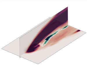
Another interesting phenomenon is that, unlike the dominant frequencies determined by the shear layer properties related to jet velocity, the dominant frequency in the non-local region remains constant for two different velocity ratios. This Strouhal number suggests wake vortex shedding, as reported by Moussa, Trischka & Eskinazi (Reference Moussa, Trischka and Eskinazi1977), who found that vortex shedding from JICF has a Strouhal number of 0.2 that is generally independent of VR. To support these observations, consider figure 12, which shows the non-local CGT regions identified using DDES and multiplane synchronized PIV/PLIF. Additionally, a snapshot of the Q criterion, coloured by ${u^{\prime}_\textrm{2}}c^{\prime}$, is depicted from a downward view. The distribution of the CGT region in the lateral direction resembles a classical wake shear layer, similar to those in the von Kármán street. The vortical structures further corroborate this observation. Thus, based on spectral characteristics, there is substantial evidence suggesting that the non-local CGT behaviour in the JICF may be associated with vortex shedding across the jet column.

Figure 12. Identification of non-local counter-gradient transport regions and visualization of the Q criterion. (a,b) Non-local counter-gradient transport regions identified using DDES and synchronized PIV/PLIF. (c,d) Snapshot of Q criterion (normalized $Q = 0.62$) coloured by ${u^{\prime}_2}c^{\prime}$ from a downward view, as determined by DDES. (a,c) $VR = 0.4$; (b,d) $VR = 1.2$.

3.3. Modelling implications

In the previous subsections, we identified locations exhibiting CGT behaviour and explored its origins. However, while insightful, the implication for turbulence modelling remains unclear. To delve into counter-gradient transport in turbulent scalar flux, we examine the angle ($\theta $) between the vectors $\overline {{u^{\prime}_i}c^{\prime}} $ and ${\partial _i}C$, expressed as

(3.6)\begin{equation}\theta = \textrm{arccos}\left( {\frac{{ - \overline {{u^{\prime}_i}c^{\prime}} {\partial_i}C}}{{|{\overline {{u^{\prime}_i}c^{\prime}} } |\cdot |{{\partial_i}C} |}}} \right).\end{equation}

In regions where the simple GDH holds precisely, $\theta $ should be $0^\circ $, indicating normal diffusion, whereas in areas exhibiting counter-gradient transport, $\theta $ exceeds $90^\circ $. Figure 13 shows contours of the angle $\theta $ at two different $VR\textrm{s}$, revealing key differences between previously identified local and non-local regions. Generally, $\theta $ is highest near the wall, where its presence induces strong anisotropy into the turbulent mixing. In the windward shear layer, where vertical turbulent motion drives local transport, $\theta $ typically ranges between $40^\circ $ and $70^\circ $, as the vertical component governed by the GDH is dominant. Conversely, regions of non-local transport, shown in figure 13(a,b), exhibit significant misalignment between $- \overline {{u^{\prime}_i}c^{\prime}} $ and ${\partial _i}C$ due to both components of the scalar flux depicting counter-gradient transport behaviour.

Figure 13. Counter-gradient transport at the mid-plane determined by synchronized PIV/PLIF. (a) $VR = 0.4$; (b) $VR = 1.2$.

From a modelling standpoint, regions where $\theta $ is significantly above zero cannot be well captured by the simple GDH described in (3.1), regardless of the diffusivity chosen. Introducing a spatially distributed $S{c_t}$ can capture some counter-gradient transport of turbulent scalar flux and would therefore be expected to model turbulent mixing more effectively. However, singular values of $S{c_t}$ could occur when $\theta > 90^\circ $ and the scalar transport equation may suffer from extreme numerical instability. Local and non-local behaviours require models of different complexity. Local behaviours can be modelled using local formulations but need a diffusivity matrix to capture cross-gradient effects (Milani et al. Reference Milani, Ling and Eaton2020). Non-local behaviours cannot be adequately modelled by any diffusivity-based model and may require solving separate transport equations for the scalar flux components. However, from a spectrum perspective, both the local and non-local behaviours correspond to large scales of the flow. The scalar flux can thus be decomposed into a gradient-type term representing the gradient diffusion and a term accounting for the stirring by large eddies. This approach extends the double-structure concept originally proposed by Townsend (Reference Townsend1976):

(3.7)\begin{equation}- \overline {{u^{\prime}_i}c^{\prime}} = \frac{{{\upsilon _t}}}{{S{c_t}}}{\partial _i}C + {( - \overline {{u^{\prime}_i}c^{\prime}} )^\ast },\end{equation}

where ${( - \overline {u^{\prime}_{i}c^{\prime}})^\ast }$ denotes the turbulent scalar flux due to large eddies.

4. Inversion framework

4.1. Model deficiency representation

The classic RANS model attempts to estimate the unknown nonlinear source term in the mean equations to acquire the mean flow quantities. For incompressible mean flow, we first define a state vector $\boldsymbol{q}$ as

(4.1)\begin{equation}\boldsymbol{q} = \left\{ {\begin{array}{@{}c@{}} p\\ {{U_i}}\\ C \end{array}} \right\},\end{equation}

where p is the static pressure of the fluid; ${U_i}$ is the mean velocity vector, $i = 1,\;2,\;3$ in a three-dimensional space; and C is the mean scalar. We may then denote ${{\mathcal R}}$ as the conserved form of the incompressible RANS models, that is,

(4.2) \begin{equation}{{\mathcal R}}(\boldsymbol{q}) = \left\{ {\begin{array}{@{}c@{}} {{\partial_j}{U_j}}\\ {\partial_j}({U_i}{U_j}) + \dfrac{1}{\rho }{\partial_i}p - \upsilon {\partial_j}{\partial_j}{U_i} + {\partial_j}\overline {u_{i}^{\prime}{u_{j}^{\prime}} }\\ {{\partial_j}({U_j}C) - {\partial_j}\left( {\dfrac{\upsilon }{{Sc}}{\partial_j}C} \right) + {\partial_j}\overline {u_{j}^{\prime}c^{\prime}} } \end{array} } \right\} = \boldsymbol{0},\end{equation}

where $Sc$ is the Schmidt number and $- \overline {{u^{\prime}_i}{u^{\prime}_j}} $ is the Reynolds stress tensor. The commonly adopted closure approximation for the second-order correlation of fluctuation states follows a form based on the classical analogies of Reynolds and GDH (Pope Reference Pope2000), assumed as

(4.3)\begin{equation}\left. {\begin{array}{c@{}} { - \overline {{u^{\prime}_i}{u^{\prime}_j}} = {\upsilon_t}{\partial_j}{U_i} - \dfrac{2}{3}k{\delta_{ij}},}\\ { - \overline {{u^{\prime}_j}c^{\prime}} = \dfrac{{{\upsilon_t}}}{{S{c_t}}}{\partial_j}C,} \end{array}} \right\}\end{equation}

where k is the turbulent kinetic energy and ${\delta _{ij}}$ is the Kronecker symbol. A constant value for $S{c_t}$ is often adopted ($S{c_t} = 0.85$ in all of the following cases). As demonstrated in §§ 2 and 3, the LEVM and GDH pose great challenges to time-averaged predictions. The solution space impedes the capability of the DA method to reproduce the second-order correlation of fluctuations. To address modelling deficiencies, we introduce a spatially distributed body force correction ${F_i}$ and ${F_C}$ into the Reynolds stress and turbulent scalar flux, as follows:

(4.4)\begin{equation}\left. {\begin{array}{c@{}} { - {\partial_j}\overline {{u^{\prime}_i}{u^{\prime}_j}} = {\partial_j}\left( {{\upsilon_t}{\partial_j}{U_i} - \dfrac{2}{3}k{\delta_{ij}}} \right) + {F_i},}\\ { - {\partial_j}\overline {{u^{\prime}_j}c^{\prime}} = {\partial_j}\left( {\dfrac{{{\upsilon_t}}}{{S{c_t}}}{\partial_j}C} \right) + {F_C}.} \end{array}} \right\}\end{equation}

The inclusion of the LEVM and GDH in (4.4) serves to enhance the effective diffusion in the RANS equations, thereby ensuring numerical stability. Indeed, DA can also be performed to optimize ${\upsilon _t}$ and $S{c_t}$. However, as demonstrated by Ling et al. (Reference Ling, Ruiz, Lacaze and Oefelein2017), singular values would occur in strongly anisotropic flow in a JICF. For non-local behaviour, the optimized coefficient of the Laplace operator is negative, generating counter-gradient transport that concentrates low-concentration regions into high-concentration regions. This can cause local increases in concentration, leading to oscillations or even blow-ups in the numerical solution. The direct assimilation of ${F_C}$ ensures robustness and convergence of the iteration in the DA process. Overall, the DA scheme demonstrates stability and convergence similar to the baseline RANS model, with instabilities occurring only when the baseline RANS computation becomes unstable. To ensure strictly divergence-free estimated force correction, we introduce the Stokes–Helmholtz decomposition as follows:

(4.5)\begin{equation}{F_i} ={-} \partial \varphi /\partial {x_i} - {\varepsilon _{ijk}}\partial {\psi _k}/\partial {x_j},\end{equation}

with the scalar potential $\varphi $, the vector potential $\psi $ and the Levi–Civita symbol ${\varepsilon _{ijk}}$. For more details on the scalar and vector potential, please refer to our previous work (Li et al. Reference Li, He and Liu2022). By substituting (4.4)–(4.5) into (4.2) and integrating the scalar potential $\varphi $ into pressure p, we have

(4.6)\begin{equation}{{\mathcal R}}(\boldsymbol{q}) = \left\{ {\begin{array}{@{}c@{}} {{\partial_j}{U_j}}\\ {{\partial_j}({U_i}{U_j}) + \dfrac{1}{\rho }{\partial_i}\bar{p} - {\partial_j}[(\upsilon + {\upsilon_t}){\partial_j}{U_i}] - {f_i}}\\ {{\partial_j}({U_j}C) - {\partial_j}\left[ {\left( {\dfrac{\upsilon }{{Sc}} + \dfrac{{{\upsilon_t}}}{{S{c_t}}}} \right){\partial_j}C} \right] - {F_C}} \end{array}} \right\} = \boldsymbol{0}.\end{equation}

Here, the modified pressure $\bar{p}$ and solenoidal part of ${F_i}$ are expressed as follows:

(4.7)\begin{equation}\left. {\begin{array}{c@{}} {\bar{p} = p + {\textstyle{2 \over 3}}k + \rho \varphi }\\ {{f_i} ={-} {\varepsilon_{ijk}}\partial {\psi_k}/\partial {x_j}} \end{array}} \right\}.\end{equation}

4.2. Continuous adjoint formulation

The DA procedure is to find the optimal forcing ${f_i}$ and ${F_C}$ by minimizing the cost function ${{\mathcal J}}$, i.e. the discrepancy between the state variables obtained by the corrected model (4.6) and the limited observations, subject to the governing equations. This is expressed as follows:

(4.8)\begin{align}\left. {\begin{array}{*{20}{c}} {{{{\mathcal J}}_{{U_i}}} = \xi \int_{{\mathcal M}} {{{{\mathcal F}}_{{x_i}}}{{\left( {\dfrac{{{U_i} - {U_{Obs,i}}}}{{{U_0}}}} \right)}^2}\textrm{d}{{\mathcal M}}} \; + \dfrac{\zeta }{2}\int_{{\mathcal M}} {{{(\,{f_i})}^2}\,\textrm{d}{{\mathcal M}}\; } }\\ {{{{\mathcal J}}_C} = {\xi_C}\int_{{\mathcal M}} {{{{\mathcal F}}_{{x_i}}}{{\left( {\dfrac{{C - {C_{Obs}}}}{{{C_0}}}} \right)}^2}\textrm{d}{{\mathcal M}}} \; + \dfrac{\zeta }{2}\int_{{\mathcal M}} {{{({F_C})}^2}\,\textrm{d}{{\mathcal M}}\; } } \end{array}}\!\!\! \right\}\quad \!\!\!\textrm{s}\textrm{.t}\textrm{.}\;{{\mathcal R}}({{{\mathcal R}}_{NS}},{{{\mathcal R}}_p},{{{\mathcal R}}_C}) = 0.\end{align}

Here, ${{\mathcal M}}$ is the computational domain; ξ and ${\xi _C}$ are dimension converter with dimensions $[{L^2} \cdot {t^{ - 3}}]$ and $[{M^2} \cdot {L^{ - 6}} \cdot {t^{ - 1}}]$, respectively, and possess a value of unity. This ensures dimensional consistency. Term ${{{\mathcal F}}_{{x_i}}}$ is a masking function that is defined to specify the region where the measurements are made. If observation data are available, ${{{\mathcal F}}_{{x_i}}} = 1$ holds; otherwise, ${{{\mathcal F}}_{{x_i}}} = 0$. Here, we incorporate knowledge on the correction force by noting that the Reynolds stress and turbulent scalar flux usually exhibit large-scale structures that vary across the length scales of the mean flow (Franceschini, Sipp & Marquet Reference Franceschini, Sipp and Marquet2020). This term penalizes undesired oscillations resulting from sparse observations. The hyperparameter $\zeta $ is introduced to balance the measurement discrepancy and smoothness of the correction. Here, ${{\mathcal R}} = {{\mathcal R}}({{{\mathcal R}}_{NS}},{{{\mathcal R}}_p},{{{\mathcal R}}_C})$ are the momentum equations, the continuity equation, and the scalar transport equation presented in (4.6), respectively.

In a variational approach, the linear equations for the small perturbations of the mean flow are used to derive the adjoint equations. We first define the adjoint state vector ${\boldsymbol{q}^\ast }$, as follows:

(4.9)\begin{equation}{\boldsymbol{q}^\ast } = \left\{ {\begin{array}{@{}c@{}} {{p^\ast }}\\ {U_i^\ast }\\ {{C^\ast }} \end{array}} \right\}.\end{equation}

To minimize the energy of the cost function, the following Lagrangian function is used:

(4.10)\begin{equation}{{\mathcal L}}(\boldsymbol{q},{\boldsymbol{q}^{\boldsymbol{\ast }}},{f_i},{F_C}) = {{\mathcal J}} + \int_{{\mathcal M}} {(U_i^\ast {{{\mathcal R}}_{NS}} + {p^\ast }{{{\mathcal R}}_p} + {C^\ast }{{{\mathcal R}}_C})\,\textrm{d}{{\mathcal M}}} .\end{equation}

The Lagrangian multipliers $U_i^\ast $, ${p^\ast }$ and ${C^\ast }$ are the adjoint variables corresponding to (4.6), and are referred to as the adjoint velocity, adjoint pressure and adjoint scalar, respectively. The optimal distribution of ${f_i}$ and ${F_C}$ can be determined by obtaining the sensitivities of the Lagrange operator ${{\mathcal L}}$ with respect to ${f_i}$ and ${F_C}$, while setting the total variations of ${{\mathcal L}}$ with respect to the other state variables to vanish, according to

(4.11)\begin{equation}\delta {{\mathcal L}} \equiv \underbrace{{{\delta _{\boldsymbol{q}}}{{\mathcal L}}}}_{0} + {\delta _{{\boldsymbol{q}^\ast }}}{{\mathcal L}} + {\delta _{{f_i}}}{{\mathcal L}} + {\delta _{{F_T}}}{{\mathcal L}}.\end{equation}

The adjoint equations can be obtained by enforcing the zero constraint in (4.11), resulting in

(4.12)\begin{align}{{{\mathcal R}}^\ast }({\boldsymbol{q}^{\boldsymbol{\ast }}}) = \left\{ {\begin{array}{@{}c@{}} {{\partial_j}U_j^\ast }\\ {U_j^\ast {\partial_i}{U_j} - {U_j}{\partial_j}U_j^\ast+ \dfrac{1}{\rho }{\partial_i}{p^\ast } - {\partial_j}[(\upsilon + {\upsilon_t}){\partial_j}{U_i}] + 2\xi {{{\mathcal F}}_{{x_i}}}\dfrac{{{U_i} - {U_{Obs,i}}}}{{{U_0}}}}\\ { - {U_j}{\partial_j}{C^\ast } - {\partial_j}\left[ {\left( {\dfrac{\upsilon }{{Sc}} + \dfrac{{{\upsilon_t}}}{{S{c_t}}}} \right){\partial_j}{C^\ast }} \right] + 2{\xi_C}{{{\mathcal F}}_{{x_i}}}\dfrac{{C - {C_{Obs}}}}{{{C_0}}}} \end{array}} \right\} = \boldsymbol{0}.\end{align}

The boundary conditions are derived as follows. For the inflow and the wall, where the primary state variable ${U_i}$, C is specified, the boundary conditions are as follows:

(4.13)\begin{equation}\left. {\begin{array}{c@{}} {U_i^\ast= \boldsymbol{0},}\\ {{n_i}{\partial_i}{p^\ast } = 0,}\\ {{C^\ast } = 0,} \end{array}} \right\}\end{equation}

where ${n_i}$ is unit surface normal vector. For the outflow boundary, where the Neumann condition is used for the primary variables, the adjoint boundary conditions are as follows:

(4.14)\begin{equation}\left. {\begin{array}{c@{}} {{U_n} \cdot U_\tau^\ast{+} (\upsilon + {\upsilon_t})({n_i}{\partial_i}{U_\tau }) = \boldsymbol{0},}\\ {{U_n} \cdot U_n^\ast{+} (\upsilon + {\upsilon_t})({n_i}{\partial_i}{U_n}) = {p^\ast },}\\ {{U_n} \cdot {C^\ast } + \left( {\dfrac{\upsilon }{{Sc}} + \dfrac{{{\upsilon_t}}}{{S{c_t}}}} \right)({n_i}{\partial_i}{C^\ast }) = 0.} \end{array}} \right\}.\end{equation}

The subscripts n and $\tau $ denote the normal and tangential components of the variables, respectively. When $\boldsymbol{q}$ and ${\boldsymbol{q}^{\boldsymbol{\ast }}}$ satisfy (4.6) and (4.12)–(4.14), the sensitivity of the Lagrange function ${{\mathcal L}}$ becomes independent of the change in the adjoint variables, such that the gradient of the cost function can be computed, as follows:

(4.15)\begin{equation}\left. {\begin{array}{c@{}} {\dfrac{{\textrm{d}{{{\mathcal J}}_{{U_i}}}}}{{\textrm{d}{f_i}}} = \dfrac{{\partial {{\mathcal L}}}}{{\partial f}} ={-} U_i^\ast{+} \zeta {F_i},}\\ {\dfrac{{\textrm{d}{{{\mathcal J}}_C}}}{{\textrm{d}{F_C}}} = \dfrac{{\partial {{\mathcal L}}}}{{\partial {F_C}}} ={-} {C^\ast } + \zeta {F_C}.} \end{array}} \right\}\end{equation}

The gradient is determined for the entire computational domain and then used to update the force correction in an optimal sense, as

(4.16)\begin{equation}\left. {\begin{array}{c@{}} {f_i^{n + 1} = f_i^n - \beta \dfrac{{\partial {{\mathcal L}}}}{{\partial {f_i}}},}\\ {F_C^{n + 1} = F_C^n - \beta \dfrac{{\partial {{\mathcal L}}}}{{\partial {F_C}}},} \end{array}} \right\}\end{equation}

where $\beta $ is the step length. The iterative framework for flow reconstruction from mean field is as follows. It begins with an initial guess for ${f_i}$ and ${F_C}$, followed by an initialization procedure where (4.6) is solved without any corrections to achieve a converged base flow for the optimization process. The force correction is then used in (4.6) to obtain the primary variable distributions. Subsequently, the adjoint equations are solved using the boundary condition (4.13)–(4.14) computed by the cost function. The adjoint solution is then used to determine the sensitivity of the Lagrangian function (4.15), which is then employed to update the correction term (4.16). Finally, the iterative loop is repeated until a convergence criterion is met.

4.3. Data assimilation set-up

The benchmark flow configuration used for DA mirrors the experiment (figure 2a), with the mainstream inlet velocity profile derived from PIV results. Nevertheless, as demonstrated in our prior work (Li et al. Reference Li, He and Liu2022), the inlet velocity profile can also be accurately computed through a precursor RANS simulation. At the outflow boundary, a Dirichlet condition is specified for pressure and a Neumann condition for velocity. The concentration field is obtained via a scalar transport model, with rhodamine's mass fraction set to $5 \times {10^{ - 8}}$ at the jet inlet and 0 at the mainstream inlet, mirroring experimental conditions. Adjoint boundary conditions align with those in (4.13)–(4.14). The convection terms in the primary-adjoint system are discretized using a linear-upwind scheme to ensure second-order accuracy. To reduce the computational mesh size whilst maintaining reasonable flow blockage, slip-wall conditions are applied to neglect boundary layer effects on the side and upper walls (Li et al. Reference Li, He and Liu2023). A structured mesh with 1.05 million grids is used for the JICF configuration after a grid independence test. Observations for assimilation are extracted from the PIV/PLIF data at the $Z/D = 0$ plane (table 1), with exclusion of the near-wall region ($d/D < 0.2$) to mimic the large uncertainty. The regularization parameter $\zeta $ is fixed at 0.001 to mitigate any spurious fluctuations in correction determination. Further insights into the impact of regularization on convergence studies can be found in our earlier work (Li et al. Reference Li, Zhang, Zhou, He and Liu2024). Validation of velocity reconstruction is presented in § 5.1, followed by the application of DA for scalar field correction in § 5.2.

Table 1. Observation set-up and regularization for various cases

5. Results and discussion

5.1. Inversion of turbulent mean flow

Figure 14 depicts the streamwise velocity distribution at two spanwise locations, $z/D = 0$ and $z/D = 0.3$. The DDES results are superimposed on the coloured contours as dashed lines for comprehensive comparison. The velocity pattern highlights both acceleration and separation at the inlet of the tube, owing to the sharp angle between the chamber and the hole. This feature is crucial for subsequent flow development. The blockage created by the flow separation induces high momentum in the upper part of the pipe, with velocities twice as high as the pipe bulk velocity. The high-shear, high-velocity region adjacent to the separation zone is particularly crucial, especially in short-hole geometries like the present one, as there is limited space for flow redevelopment before interacting with the mainstream. Additionally, the substantial disparity in velocity between $z = 0$ and $z = 0.4D$ suggests the presence of a pronounced secondary flow within the pipe. The counter-rotating vortices developing inside the hole may interact with the well-known counter-rotating vortex pair (CRVP) that dominates every JICF.

Figure 14. Streamwise velocity distribution at two spanwise locations: (a,c) $\; z/D\; = \; 0$ and (b,d) $z/D\; = \; 0.3$. Colour contours show SA estimation and data assimilation based on SA (DA-SA), with DDES results overlaid as lines for reference. (a,b) $VR = 0.4$; (c,d) $VR = 1.2$.

A thorough examination reveals two notable distinctions between the default SA model and the reference. In zone I, a disparity in the pattern of the jet core is evident in the streamwise velocity. The reference exhibits a wider and shorter jet core, while the default SA model predicts a narrower core compressed into the upstream region of the jet. In zone II, downstream of the jet leeward, the streamwise velocity determined by the default SA model exhibits a more pronounced decay rate compared with the reference. Both disparities indicate that the default SA model tends to underestimate the diffusion in the JICF. The first discrepancy arises from the jet separation at the hole inlet, and the second is attributed to the adverse pressure gradient from the test plate.

As depicted in figure 14, the reconstructed velocity exhibits a notable enhancement within the region available for observation after DA, consistent with expectations. The low-speed region downstream of the jet's exit is reduced compared with that for the default SA model. It is worth noting that the DA procedure accurately recovers the streamwise velocity at plane $z/D = 0.3$, despite only mid-plane observations being used. This successful correction primarily stems from the global correction mechanism embedded within the DA scheme. This mechanism relies on both the upstream convection of the adjoint velocity and the downstream convection of the primary flow. Initially, all adjoint values remain at zero until the system is triggered by the source term in (4.12), defined as the disparity between observations and predictions. Subsequently, upon excitation, the adjoint solution evolves in reverse direction based on the primary solution. The disturbance, induced by the convective velocity, propagates through the control region, providing essential information for computing the gradient (4.15), and thus the correction force.

To further elucidate the underlying mechanism of the improvement, we examine the distributions of normalized eddy viscosity before and after DA at mid-plane$\; z/D\; = \; 0$ and axial plane $x/D = 4$, as depicted in figure 15. It is evident that the eddy viscosity experiences a significant increase after DA, both within the jet hole (region I) and the mixing layer (region II). This notable rise in eddy viscosity introduces additional diffusion, thereby enhancing momentum exchange within the shear layer.

Figure 15. Distribution of eddy viscosity (a,b) before, (c,d) after DA at mid-planes $z/D\; = \; 0$ and axial planes $x/D = 4$. (a,c) $VR = 0.4$; (b,d) $VR = 1.2$.

A profound understanding of the improvement lies in the redistribution of the Reynolds stress forcing ${R_i}$, expressed as

(5.1)\begin{equation}{R_i} ={-} {\partial _j}\overline {{u^{\prime}_i}{u^{\prime}_j}} = {\partial _j}({\upsilon _t}{\partial _j}{U_i} - {\textstyle{2 \over 3}}k{\delta _{ij}}) + {F_i}.\end{equation}

The streamwise Reynolds stress forcing ${R_1}$ at two spanwise locations is depicted in figure 16. In the SA model, the streamwise Reynolds stress forcing in the shear layer is notably underestimated in both the tube and cross-flow regions. This underestimation results in a lower effective viscosity, consequently leading to a substantial recirculation region both in the tube and downstream of the jet leeward. In contrast, the DA model exhibits a substantial increase in the streamwise Reynolds stress forcing within the tube, both windward and leeward of the shear layer. This augmentation contributes additional vorticity to the interaction between the mainstream and jet flow, enhancing effective viscosity.

Figure 16. Full Reynolds stress forcing ${R_1}$ at mid-planes$\; z/D\; = \; 0$ and axial planes $x/D = 4$, obtained by (a,b) the SA model, (c,d) DA based on SA (DA-SA) and (ef) DDES results. (a,c,e) $VR = 0.4$; (b,df) $VR = 1.2$.

5.2. Exploration of the concentration field

In film cooling and many other JICF applications, the mixing behaviours are highly concerned. Achieving an accurate representation of mean mixing behaviour hinges not only on understanding Reynolds stress but also on grasping turbulent scalar flux. This prompts a crucial question: does an accurate velocity field necessarily imply an accurate scalar field? And if not, does it yield any enhancements? Furthermore, what physical mechanisms enable adjoint-based DA to enhance the reconstruction accuracy? Therefore, further investigation of applying the adjoint-based DA to correct the concentration field is conducted.

Figures 17 and 18 depict concentration distributions at mid-planes, wall-normal planes and axial planes obtained using different models: the default SA, DA-SA (using PIV measurements as observations) and DA-SA-C (incorporating both PIV and PLIF measurements as observations). In figure 17, DDES results, validated against experimental data, are overlaid on the coloured contours as dashed lines for comparison. The concentration field predicted by the default SA model (figure 17a,b) shows an underestimation of turbulent mixing throughout much of the domain, particularly near the wall. Additionally, as depicted in figure 18(a,c), the concentration gradient in the shear layer is steeper than the reference, indicating an underestimation of lateral mixing between the jet and cross-flow, causing the jet scalar to penetrate deeper into the mainstream compared with DDES and experimental results. This deeper penetration is influenced by both convective and turbulent scalar flux transport, driven by Reynolds stress and turbulent scalar flux, respectively. The limited turbulent viscosity in the SA model, due to the LEVM, results in insufficient turbulent diffusion, as prescribed by the GDH with a fixed turbulent Schmidt number. Interestingly, for the higher velocity ratio ($VR\; = \; 1.2$), the jet centreline mean scalar prediction aligns more closely with the reference, as shown in figure 17(b) and in the profiles of figure 17(h). This suggests that in the higher $VR$ case, the isotropic formulation of the GDH is more appropriate, likely because the jet is further from the wall, making spanwise and wall-normal transport more similar. In contrast, in the lower $VR$ case, the jet remains closer to the wall, which suppresses vertical eddies and increases turbulence anisotropy, making the isotropic GDH formulation less accurate.

Figure 17. Concentration distribution at mid-planes obtained by (a,b) SA estimation, (c,d) DA based on SA (DA-SA), and (ef) DA with scalar flux correction based on SA (DA-SA-C). White dashed lines, DDES results. (a,c,e,g) $VR = 0.4$; (b,df,h) $VR = 1.2$.

Figure 18. Concentration at wall-normal (left, $y/D\; = \; 0.5$ for $VR = 0.4$ and $y/D\; = \; 1.0$ for $VR = 1.2$) and axial planes (right, $x/D\; = \; 4$ for $VR = 0.4$ and $x/D\; = \; 2.5$ for $VR = 1.2$). (a,b) $VR = 0.4$; (c,d) $VR = 1.2$.

Figures 17(c,d) and 18(b,d) depict the concentration distribution determined by the DA-SA model. Despite incorporating a reconstructed velocity distribution and an improved eddy viscosity estimation in the scalar transport equation, the results from the DA-SA model reveal minimal correction (figures 17d and 18d) or even a deterioration in performance (figures 17c and 18b) for both $VR = 0.4$ and $1.2$. A detailed line profile comparison in figure 17(g,h) starkly illustrates this trend, showing marginal or no discernible improvement. Further scrutiny of the distribution highlights nuanced improvements in the scalar field. Specifically, for the $VR = 0.4$ case, the DA-SA model exhibits better alignment with the centreline trajectory position observed in DDES results. For $VR = 1.2$, increased turbulence diffusion moderately enhances concentration decay, particularly noticeable where $x/D < 2$ (figures 17d and 18d).

The scalar distribution in the DA-SA model results from the interplay between enhanced convective transport and increased turbulent diffusion. Both velocity ratios of DA-SA exhibit improved streamwise convective transport (see figures 14 and 4ad), enhancing scalar penetration along the streamwise direction. Additionally, increased eddy viscosity (figure 15) enhances mixing efficiency. Specifically, for $VR = 0.4$ at the mid-plane, convective transport dominates, elongating the scalar distribution along the streamwise centreline and penetrating deeper into the cross-flow compared with SA model predictions. In contrast, for $VR = 1.2$, turbulent diffusion prevails, contributing to varying degrees of improvement.

As we transition to the wall-normal direction, improvements in the DA-SA results become more intricate. Despite applying enhanced velocity and eddy viscosity, improvements in the DA-SA model's scalar distribution are not guaranteed. Our observations indicate that while the DA-SA model enhances certain aspects of the flow, such as the scalar distribution within the jet core and the concentration gradient in the shear layer, these improvements do not consistently extend to the downstream scalar distribution. This discrepancy is primarily attributed to the competing effects of convective transport and turbulent diffusion. This nuanced perspective underscores that while the DA-SA model introduces refinements, particularly in alignment and diffusion characteristics, significant improvements in scalar distribution across all tested conditions remain elusive.

Simply improving the velocity and eddy viscosity fields yield only marginal improvements in correcting the concentration field. Thus, we used the adjoint-based DA, integrating both PIV and PLIF data (DA-SA-C). Figure 17(ef) showcases the concentration distribution at the mid-planes determined by the DA-SA-C model. Impressively, the reconstructed scalar field closely mirrors the results obtained from the DDES, spanning both the observation-embedded and unseen regions. Two notable improvements stand out. First, the windward shear layer concentration distribution displays remarkable improvement, showcasing an augmented mixing, as depicted in figure 17(ef). This enhancement is further emphasized in the wall-normal scalar distribution, particularly evident in the $VR = 1.2$ case, as illustrated in figure 18(b,d). Second, the decay rate of the concentration distribution in both the streamwise and spanwise direction is captured. However, subtle deviations persist, notably in the core region of the CRVP in figure 18(b,d), possibly stemming from inconsistencies between DDES and PIV/PLIF measurements.

Spanwise-averaged line plots provide a more quantitative comparisons between various models and the PLIF results. Figure 19 demonstrates spanwise-averaged vertical concentration profiles at three measurement planes ($z/D = 0$, $z/D = 0.3$ and $z/D = 0.5$) at different stations. The black circles represent the PLIF data, serving as the benchmark for model validation. Once again, the limitations of the default SA model are evident: an excessively small diffusivity sharpens the profile, overestimates values near the jet centreline and shifts the scalar peak downwards. As expected, the predictions from the DA-SA model exhibit a moderate enhancement, especially in the vicinity of the jet centreline. This improvement is primarily ascribed to the augmented viscosity, thereby leading to an increase in turbulent diffusivity. However, a remarkable deviation persists in the near-wall region due to strong wall-induced anisotropy. Incorporating both PIV and PLIF results into the DA model yields excellent concentration predictions, as showcased in figure 19. The comprehensive improvements underscore the capability of the adjoint-based DA approach in capturing underlying mechanisms and enact effective modifications.

Figure 19. Spanwise-averaged ($z/D = 0$, $z/D = 0.3$ and $z/D = 0.5$) concentration distribution at different stations. The DA-SA-Sc model denotes the scalar transport simulation with a constant turbulent Schmidt number of 0.32 from Zhang et al. (Reference Zhang, Wang, Zhou, He and Liu2023b). (ad) $VR = 0.4$; (eh) $VR = 1.2$.

To further elucidate the enhanced turbulent mixing, we performed a simulation using velocity and eddy viscosity reconstructed through the DA procedure, along with a constant turbulent Schmidt number set at 0.32. This turbulent Schmidt number was determined by an EnKF-based DA method for JICF mixing (Zhang et al. Reference Zhang, Wang, Zhou, He and Liu2023b). The turbulent Schmidt number is a version of the turbulent diffusivity, ${\alpha _t}$, scaled by the local eddy viscosity:

(5.2)\begin{equation}S{c_t} = {\upsilon _t}/{\alpha _t}.\end{equation}

For $S{c_t} < 1$, decreasing $S{c_t}$ equates to an endeavour to bolster turbulent mixing in scalar transportation. Figure 19 shows that decreasing the turbulent Schmidt number results in a significant improvement in scalar distribution when $x/D < 6$. The improvement in the present DA approach resembles similar corrective behaviour as reducing the turbulent Schmidt number, as also observed by Zhang et al. (Reference Zhang, Mao, Su and Yuan2022b). However, this reduction in $S{c_t}$ introduces too much diffusivity to the scalar transport equation for the far field, resulting in a smoothed vertical profile. For the present DA approach, despite observations being available only in the region $x/D \in [0,4]$ at the mid-plane, the downstream scalar distribution still demonstrates a remarkable improvement. One potential reason is the effect of anisotropy in the turbulent transport. In the near-field region, the jet remains closer to the wall, which acts to damp vertical eddies and thus renders turbulence more anisotropic. As the jet progresses further downstream from the wall, as in the region $x/D > 6$, spanwise and wall-normal transport are probably more similar, so the isotropic formulation of the GDH becomes a better approximation. This physical transition can be accurately discerned from the global correction mechanism embedded within the DA scheme.

Figure 20 illustrates the distributions of the adjoint scalar obtained from different $VR\textrm{s}$ before and after DA. The adjoint scalar before the gradient descent optimization approximately represents the deviations induced by the model deficiency. Initially, all adjoint values are set to zero until the system is excited by the source term in (4.12), defined as the disparity between the PLIF measurements and model estimates. After excitation, the adjoint solution evolves in the reverse direction, based on the primary solution. The disturbance, dictated by the convective velocity, propagates through the control region, offering information for computing the gradient (4.15). The large magnitudes of the adjoint scalar in figure 20 underscore the heightened sensitivity of the flow to the measurements. Specifically, the adjoint scalar remains exhibits significant magnitudes proximal to both windward and leeward shear layers, alongside the near-wall regions, mirroring the deficiencies observed in figure 13. It is noteworthy that all the adjoint scalar (figure 20c,d) decrease to extremely small values as the computation converges. This convergence eliminates the disparity between estimates and observations, which serves as the source in the adjoint equations.

Figure 20. Distribution of the adjoint scalar at the mid-plane ($z/D = 0$) and wall-normal plane ($\,y/D = 0.25$) (a,b) before and (c,d) after DA. (a,c) $VR = 0.4$; (b,d) $VR = 1.2$.

It is important to note that inaccuracies in scalar transport predictions are not limited to CGT alone. The errors in predicting turbulent scalar flux using the GDH model primarily stem from two factors. First, model form uncertainty, particularly related to local and non-local CGT behaviours as discussed in § 3.2. The simple, isotropic GDH model is inadequate for accurately describing this process. Second, even in the absence of CGT, a fixed turbulent Schmidt number is insufficient for representing the shear layer turbulent scalar mixing. Figures 17(a,b) and 18(a,c) clearly show that the scalar field predicted by the default SA model underestimates turbulent mixing throughout much of the jet centreline. This results in the jet scalar penetrating deeper into the mainstream compared with the DDES and experimental results.

The forcing term added to the scalar equation is designed to correct the modelled scalar flux, ensuring it better aligns with observational data. Although the derived forcing term does not directly provide the turbulent scalar flux, it highlights regions where the GDH model deviates from expected behaviours. Physically, the turbulent scalar flux quantifies how turbulence redistributes scalar quantities, leading to mixing within the flow. The Laplacian of a scalar field typically represents the local concavity or convexity and the local rate of change at a particular point, which is often used to analyse the diffusion properties or transport behaviour of the scalar within a medium. To better understand the correction force, the derived forcing term is expressed as proportional to the Laplacian of the scalar field:

(5.3)\begin{equation}{F_C} = {\alpha ^\ast }{\nabla ^2}C.\end{equation}

Here, the Laplacian ${\nabla ^2}C$ measures the diffusion of the scalar concentration through the fluid. When ${\nabla ^2}C$ is positive, C is ‘concave up’, indicating a local minimum where the scalar value at the point is lower than the average of its neighbours, resulting in a net influx of the scalar. Conversely, when ${\nabla ^2}C$ is negative, C is ‘concave down’, indicating a local maximum where the scalar value is higher than the average of its neighbours, resulting in a net outflux.

Figure 21 presents the distributions of the coefficient ${\alpha ^\ast }$ and the Laplacian ${\nabla ^2}C$, recomputed from the correction force ${F_C}$ after DA. The results demonstrate that the forcing term effectively identifies areas where the traditional GDH falls short, particularly in the jet centreline and near-wall regions. In regions where ${\alpha ^\ast } > 0$, scalar diffusion is governed by ${\nabla ^2}C$. In the jet centreline, the correction acts as a sink (${\alpha ^\ast }{\nabla ^2}C < 0$), making the scalar to diffuse remarkably away and reducing the local concentration. This observation aligns with the results shown in figures 17 and 18. The GDH, which uses a fixed turbulent Schmidt number of 0.85, is based on boundary layer studies and tends to underestimate turbulent mixing. Previous work suggests that $S{c_T} \approx 0.85$ is appropriate for the turbulent boundary layer, while $S{c_T} \approx 0.7$ is more suitable for the jet core region (Durbin & Reif Reference Durbin and Reif2010). Enhanced turbulent mixing in the jet core region is primarily driven by large turbulent structures. As demonstrated in § 3.1, these structures shed from regions near the jet centreline, leading to significant mass exchange and enhanced turbulent mixing compared with that at the boundary layers. This finding is consistent with the experimental results of Koeltzsch (Reference Koeltzsch2000), who reported a smaller turbulent Schmidt number near the jet centreline compared with the boundary layer.

Figure 21. Colour contours of (ad) the coefficient ${\alpha ^\ast }$ at the wall-normal ($\,y/D = 0.25$) and mid-plane ($z/D = 0$), and (e,f) the Laplacian of the scalar field ${\nabla ^2}C$ at the mid-plane ($z/D = 0$). (a,c,e) $VR = 0.4$; (b,df) $VR = 1.2$.

Other improvements are observed in the windward shear layer downstream of the jet orifice, where ${\alpha ^\ast }{\nabla ^2}C$ depicts a positive value, serving as a source for the mean scalar. This reduces local turbulent mixing and increases the local scalar value, as depicted in figures 17(h) and 19(ef). A similar correction force is observed in the leeward shear layer, although it does not fully align with the scalar field correction. This inconsistency may be due to the low magnitude of ${\alpha ^\ast }$ in those regions, making the diffusivity negligible and allowing the reduction of scalar concentration in the jet centreline to dominate. It is important to note that while the posterior results in the windward shear layer show reasonable improvement, the implications of the correction force for local cross-gradient CGT behaviour are difficult to identify due to the divergence operation on the turbulent scalar flux. However, as demonstrated in Appendix A, while this cross-gradient CGT behaviour is interesting from a physical perspective, it does not significantly impact the mean scalar concentration.

Transitioning from this analysis, it is crucial to highlight the impact of negative ${\alpha ^\ast }$ values in other critical regions. Notably, just above the wall post-injection, negative values of ${\alpha ^\ast }$ emerge both in the mid-plane and wall-normal directions, aligning with regions characterized by non-local CGT behaviour. In these regions, the Laplacian term ${\nabla ^2}C$ is positive, indicating a ‘concave up’ scalar field where gradient diffusion would typically increase local concentration by drawing scalar from surrounding regions. However, the negative ${\alpha ^\ast }$ coefficient leads to a reversal of this process, making scalar flux to diffuse away from the region, reducing the local scalar concentration and highlighting the non-local CGT behaviour. Such negative coefficients are challenging to obtain using the traditional modelling approach. This nuanced understanding underscores the DA model's ability to not only capture CGT transport effectively, but also to improve the prediction of mixing in the shear layer, thereby explaining its superior performance over the baseline model.

Similar to the Reynolds stress forcing, the turbulent scalar force ${R_C}$, which represents the contribution of turbulence to the scalar diffusion, is expressed as

(5.4)\begin{equation}{R_C} ={-} {\partial _j}\overline {{u^{\prime}_j}c^{\prime}} = {\partial _j}\left( {\frac{{{\upsilon_t}}}{{S{c_t}}}{\partial_j}C} \right) + {F_C}.\end{equation}

The resulting turbulent scalar force ${R_C}$ at the wall-normal and axial planes is presented in figure 22. In the default GDH model, the magnitude of the turbulent scalar force is significantly underestimated in both the jet centreline and CRVP regions. The underestimation of turbulent scalar force in the jet centreline leads to reduced mixing, as depicted in figures 17 and 18. The underestimation of turbulent scalar force in the CRVP region is more pronounced and contributes to most of the deficiencies in the GDH model. The CRVP is a dominant feature of the JICF flow under most conditions because it is clearly visible in the mean field. It consists of axial vortices with a common-up direction that distort the shape of the jet core as they advect downstream. The CRVP plays a crucial role in mixing the jet and cross-flow, especially near the wall, and thus is important in JICF applications. Regarding the DA-SA model, as demonstrated in the upper part of figure 22(b,d), the structure of the ${R_C}$ closely resembles the default GDH model, with a slight increase in magnitude observed in both the shear layer and the CRVP region. This increase primarily stems from enhanced dissipation induced by velocity reconstruction. In contrast, DA-SA-C accurately computes ${R_C}$ compared with the ground truth (DDES results), consistent with the agreement of the mean scalar fields between DA-SA-C and DDES/PLIF (figures 17 and 18). The DA-SA-C model shows a substantial increase in the magnitude of the ${R_C}$, especially in the CRVP region, providing additional mixing for the CRVP.

Figure 22. Full turbulent scalar force ${R_C}$ obtained at the wall-normal planes (left, $y/D\; = \; 0.5$ for $VR = 0.4$ and $y/D\; = \; 1.0$ for $VR = 1.2$) and axial planes (right, $x/D\; = \; 4$ for $VR = 0.4$ and $x/D\; = \; 2.5$ for $VR = 1.2$). (a,b) $VR = 0.4$; (c,d) $VR = 1.2$.

Line distribution of the full turbulent scalar force ${R_C}$ along the streamwise curve is presented in figure 23. The DA-SA-Sc results are also overlaid for comprehensive comparison. Compared with the DDES results, the default SA model shows a clear underestimation of the turbulent scalar force. The DA-SA model closely resembles the profile of the default SA model with a moderate increase in magnitude. In contrast, the profile of ${R_C}$ in the DA-SA-C model more closely matches the DDES results. Although the DA-SA-Sc model presents an overly smoothed estimation of concentration, the reconstructed ${R_C}$ suggests a common trend in both the DA-SA and DA-SA-C models: enhanced mixing attributed to the heightened magnitude of turbulent scalar force, as the arrow shown in figure 23. Another interesting observation is that as the jet develops further downstream from the wall ($x/D > 6$), all profiles except the DA-SA-Sc converge to the default GDH with a constant $S{c_t} = 0.85$. This suggests that the spanwise and wall-normal transport of scalar flux become more similar, making the isotropic formulation of the default GDH a better approximation. This physical transition, identified from the global correction of ${R_C}$, underscores the accuracy of the second-order momentum recovery using the present formulation, which is critically important for the mean field reproduction.

Figure 23. Distribution of full turbulent scalar force ${R_C}$ along the curve $y/D = 0.5$ for (a) $VR = 0.4$ and $y/D = 1.0$ for (b) $VR = 1.2$ at the mid-plane. The DA-SA-Sc model refers to the scalar transport simulation with a constant turbulent Schmidt number of 0.32 from Zhang et al. (Reference Zhang, Wang, Zhou, He and Liu2023b).

6. Conclusions

The present study offers a twofold contribution on counter-gradient transport of turbulent scalar flux. First, we employed an inclined JICF under two distinct flow regimes to elucidate the underlying driving mechanism in regions exhibiting CGT behaviour. Second, we delve into the reconstruction of turbulent mean flow and scalar field using continuous adjoint data assimilation with limited observations. By examining turbulent scalar mixing through synchronized PIV and PLIF measurements, we clarified the previously observed but unexplained phenomenon of CGT, revealing key flow structures, their spatial distribution and modelling implications. Statistical analysis reveals two distinct types of CGT behaviours in JICF. The first, occurring in the windward shear layer, is primarily driven by local cross-gradient transport. This is consistent with the report of previous work (Milani et al. Reference Milani, Ling and Eaton2020). The second type, identified near the wall following injection, is governed by non-local effects, resulting in a positive vertical scalar flux despite negative scalar fluctuation variance production. These CGT behaviours are closely associated with specific flow structures, namely K–H vortices (local) and wake vortices (non-local), that govern scalar flux transport across different flow regions. These findings highlight the varying levels of complexity in turbulence models. However, from a spectrum perspective, both the local and non-local behaviours correspond to the large scales of the flow. Consequently, the scalar flux can be decomposed into a gradient-diffusion term and a term representing large-eddy stirring.

Thus, an adjoint DA scheme has been established for reconstructing turbulent mean flow and scalar field. Model-form errors stemming from the Boussinesq approximation and the GDH are rectified through anisotropic correction under the constraint of observational data. The DA model is theoretically derived to minimize discrepancies between PIV/PLIF measurements and numerical predictions, thereby enabling the determination of the optimal contribution of the Reynolds force vector and turbulent scalar force. As expected, the introduced forcing term effectively identifies regions where traditional models fall short, particularly in the jet centreline and near-wall areas, thereby enhancing the accuracy of the mean scalar field not only within the observation region but also in unseen regions.

These findings underscore the reliability and practicality of the DA model in replicating mean flow behaviours from limited observations. By focusing on the divergence of turbulent scalar flux, we leverage the double structure concept (Townsend Reference Townsend1976) to improve modelling accuracy. This approach introduces new machine learning targets – specifically, the divergence of the nonlinear component of turbulent scalar flux – which can be integrated into neural networks for model consistent turbulence modelling (Brunton et al. Reference Brunton, Noack and Koumoutsakos2020) across various JICF configurations. Targeting a divergence field offers a data-driven advantage over vector fields, as it requires learning fewer components. Ongoing work seeks to integrate this strategy with physical invariance in the RANS system. This framework, inspired by Ling, Kurzawski & Templeton (Reference Ling, Kurzawski and Templeton2016), paves the way for a robust data-driven turbulence model capable of accurately predicting complex flow phenomena like film cooling.

Funding

The authors gratefully acknowledge financial support for this study from the National Natural Science Foundation of China (12227803, 12402337).

Declaration of interests

The authors report no conflict of interest.

Appendix A. Relative contribution of the scalar flux

The forcing term added to the scalar equation is designed to correct the modelled scalar flux, ensuring it better aligns with observational data. Since this forcing term acts as a divergence correction on the turbulent scalar flux, understanding its physical implications requires examining the relative contributions of the turbulent scalar flux components to the mean field. The scalar transport equation typically balances mean advection and turbulent scalar flux, assuming negligible molecular diffusion, as shown in

(A1)\begin{equation}{\partial _j}({U_j}C) = {\partial _j}\overline {{u^{\prime}_j}c^{\prime}} .\end{equation}

In a jet in cross-flow, the streamwise length scales and mean velocities are much larger than those in the transverse directions, making the streamwise mean advection generally balance turbulent mixing in the transverse directions. As a result, errors in the transverse components of turbulent scalar flux ($\overline {{u^{\prime}_2}c^{\prime}} $ and $\overline {{u^{\prime}_3}c^{\prime}} $) have a more significant impact on the mean scalar field computed through RANS than errors in the streamwise component ($\overline {{u^{\prime}_1}c^{\prime}} $). Figure 24 shows the magnitude of turbulent scalar flux components relative to the mean advection component from the synchronized PIV/PLIF. It reveals that $\overline {{u^{\prime}_2}c^{\prime}}$ is more prominent than $\overline {{u^{\prime}_1}c^{\prime}} $, with high magnitudes observed in the windward shear layer around the jet and near the wall after injection. This suggests that, while local CGT is physically interesting, as discussed in § 3.2, it does not significantly contribute to the mean flux divergence. In contrast, the wall-normal flux is critical in shaping the mean flux divergence, thereby directly influencing the mean scalar equation.

Figure 24. Magnitude of turbulent scalar flux components relative to the equivalent mean advection component determined by PIV/PLIF. (a,b) Streamwise component $|{\overline {u_{\textrm{1}}^{\prime}c^{\prime}}}/{U_1}C |$ and (c,d) wall-normal component $|{\overline {u_{\textrm{2}}^{\prime}c^{\prime}}} /{U_2}C |$.

References

Azzi, A. & Lakehal, D. 2001 Perspectives in modelling film-cooling of turbine blades by transcending conventional two-equation turbulence models. ASME Intl Mech. Engng Congr. Expo. 35623, 335347.Google Scholar
Bergeles, G., Gosman, A.D. & Launder, B.E. 1978 The turbulent jet in a cross stream at low injection rates: a three-dimensional numerical treatment. Numer. Heat Transfer B Fundam. 1, 217242.CrossRefGoogle Scholar
Bodart, B.J., Coletti, F. & Eaton, J.K. 2013 High-fidelity simulation of a turbulent inclined jet in a crossflow. Cent. Turbul. Res. Annu. Res. Briefs 19, 263275.Google Scholar
Brener, B.P., Cruz, M.A., Thompson, R.L. & Anjos, R.P. 2021 Conditioning and accurate solutions of Reynolds average Navier–Stokes equations with data-driven turbulence closures. J. Fluid Mech. 915, A110.CrossRefGoogle Scholar
Brunton, S.L., Noack, B.R. & Koumoutsakos, P. 2020 Machine learning for fluid mechanics. Annu. Rev. Fluid Mech. 52, 477508.CrossRefGoogle Scholar
Duraisamy, K., Iaccarino, G. & Xiao, H. 2019 Turbulence modeling in the age of data. Annu. Rev. Fluid Mech. 51, 357377.CrossRefGoogle Scholar
Durbin, P.A. 2018 Some recent developments in turbulence closure modeling. Annu. Rev. Fluid Mech. 50, 77103.CrossRefGoogle Scholar
Durbin, P.A. & Reif, B.A.P. 2010 Statistical Theory and Modeling for Turbulent Flows. John Wiley & Sons.CrossRefGoogle Scholar
Foures, D., Dovetta, N., Sipp, D. & Schmid, P.J. 2014 A data-assimilation method for Reynolds-averaged navier-stokes-driven mean flow reconstruction. J. Fluid Mech. 759, 404431.CrossRefGoogle Scholar
Franceschini, L., Sipp, D. & Marquet, O. 2020 Mean-flow data assimilation based on minimal correction of turbulence models: application to turbulent high Reynolds number backward-facing step. Phys. Rev. Fluids 5, 094603.CrossRefGoogle Scholar
Hafez, A.M., Abd El-Rahman, A.I. & Khater, H.A. 2022 Field inversion for transitional flows using continuous adjoint methods. Phys. Fluids 34, 124110.CrossRefGoogle Scholar
Hamba, F. 2022 Analysis and modelling of non-local eddy diffusivity for turbulent scalar flux. J. Fluid Mech. 950, A38.CrossRefGoogle Scholar
He, C., Liu, Y. & Yavuzkurt, S. 2017 A dynamic delayed detached-eddy simulation model for turbulent flows. Comput. Fluids 146, 174189.CrossRefGoogle Scholar
He, C., Wang, P. & Liu, Y. 2021 Data assimilation for turbulent mean flow and scalar fields with anisotropic formulation. Exp. Fluids 62, 117.CrossRefGoogle Scholar
Heitz, D., Mémin, E. & Schnörr, C. 2010 Variational fluid flow measurements from image sequences: synopsis and perspectives. Exp. Fluids 48, 369393.CrossRefGoogle Scholar
Kato, H., Yoshizawa, A., Ueno, G. & Obayashi, S. 2015 A data assimilation methodology for reconstructing turbulent flows around aircraft. J. Comput. Phys. 283, 559581.CrossRefGoogle Scholar
Kays, W.M. 1994 Turbulent Prandtl number. Where are we? J. Heat Transfer 116, 284295.CrossRefGoogle Scholar
Koeltzsch, K. 2000 The height dependence of the turbulent Schmidt number within the boundary layer. Atmos. Environ. 34, 11471151.CrossRefGoogle Scholar
Komori, S., Ueda, H., Gino, F. & Mizushina, T. 1983 Turbulence structure in stably stratified open-channel flow. J. Fluid Mech. 130, 1326.CrossRefGoogle Scholar
Kraichnan, R.H. 1970 Diffusion by a random velocity field. Phys. Fluids 13, 2231.CrossRefGoogle Scholar
Lakehal, D., Theodoridis, G.S. & Rodi, W. 2001 Three-dimensional flow and heat transfer calculations of film cooling at the leading edge of a symmetrical turbine blade model. Intl J. Heat Fluid Flow 22, 113122.CrossRefGoogle Scholar
Li, N., Balaras, E. & Wallace, J.M. 2010 Passive scalar transport in a turbulent mixing layer. Flow Turbul. Combust. 85, 124.CrossRefGoogle Scholar
Li, S., He, C. & Liu, Y. 2022 A data assimilation model for wall pressure-driven mean flow reconstruction. Phys. Fluids 34, 015101.CrossRefGoogle Scholar
Li, S., He, C. & Liu, Y. 2023 Unsteady flow enhancement on an airfoil using sliding window weak-constraint four-dimensional variational data assimilation. Phys. Fluids 35, 065122.CrossRefGoogle Scholar
Li, S., Zhang, X., Zhou, W., He, C. & Liu, Y. 2024 Particle image velocimetry, delayed detached eddy simulation and data assimilation of inclined jet in crossflow. J. Vis. 27, 307322.CrossRefGoogle Scholar
Li, X., Qin, Y., Ren, J. & Jiang, H. 2014 Algebraic anisotropic turbulence modeling of compound angled film cooling validated by particle image velocimetry and pressure sensitive paint measurements. J. Heat Transfer 136, 032201.CrossRefGoogle Scholar
Li, Z., Hoagg, J.B., Martin, A. & Bailey, S.C.C. 2018 Retrospective cost adaptive Reynolds-averaged Navier–Stokes kω model for data-driven unsteady turbulent simulations. J. Comput. Phys. 357, 353374.CrossRefGoogle Scholar
Li, Z., Zhang, H., Bailey, S.C.C., Hoagg, J.B. & Martin, A. 2017 A data-driven adaptive Reynolds-averaged Navier–Stokes kω model for turbulent flow. J. Comput. Phys. 345, 111131.CrossRefGoogle Scholar
Ling, J., Kurzawski, A. & Templeton, J. 2016 Reynolds averaged turbulence modelling using deep neural networks with embedded invariance. J. Fluid Mech. 807, 155166.CrossRefGoogle Scholar
Ling, J., Rossi, R. & Eaton, J.K. 2015 Near wall modeling for trailing edge slot film cooling. J. Fluids Engng 137, 021103.CrossRefGoogle Scholar
Ling, J., Ruiz, A., Lacaze, G. & Oefelein, J. 2017 Uncertainty analysis and data-driven model advances for a jet-in-crossflow. J. Turbomach. 139, 021008.CrossRefGoogle Scholar
Liu, C.L., Zhu, H.R. & Bai, J.T. 2008 Effect of turbulent Prandtl number on the computation of film-cooling effectiveness. Intl J. Heat Mass Transfer 51, 62086218.CrossRefGoogle Scholar
Liu, C.L., Zhu, H.R. & Bai, J.T. 2011 New development of the turbulent Prandtl number models for the computation of film cooling effectiveness. Intl J. Heat Mass Transfer 54, 874886.CrossRefGoogle Scholar
Mahesh, K. 2013 The interaction of jets with crossflow. Annu. Rev. Fluid Mech. 45, 379407.CrossRefGoogle Scholar
Milani, P.M., Ling, J. & Eaton, J.K. 2020 Turbulent scalar flux in inclined jets in crossflow: counter gradient transport and deep learning modelling. J. Fluid Mech. 906, A27.CrossRefGoogle Scholar
Moussa, Z.M., Trischka, J.W. & Eskinazi, S. 1977 The near field in the mixing of a round jet with a cross-stream. J. Fluid Mech. 80, 4980.CrossRefGoogle Scholar
Muppidi, S. & Mahesh, K. 2008 Direct numerical simulation of passive scalar transport in transverse jets. J. Fluid Mech. 598, 335360.CrossRefGoogle Scholar
Pfadler, S., Kerl, J., Beyrau, F., Leipertz, A., Sadiki, A., Scheuerlein, J. & Dinkelacker, F. 2009 Direct evaluation of the subgrid scale scalar flux in turbulent premixed flames with conditioned dual-plane stereo PIV. Proc. Combust. Inst. 32, 17231730.CrossRefGoogle Scholar
Pope, S.B. 2000 Turbulent Flows. Cambridge University Press.Google Scholar
Salewski, M., Stankovic, D. & Fuchs, L. 2008 Mixing in circular and non-circular jets in crossflow. Flow Turbul. Combust. 80, 255283.CrossRefGoogle Scholar
Sau, R. & Mahesh, K. 2008 Dynamics and mixing of vortex rings in crossflow. J. Fluid Mech. 604, 389409.CrossRefGoogle Scholar
Schreivogel, P., Abram, C., Fond, B., Straußwald, M., Beyrau, F. & Pfitzner, M. 2016 Simultaneous kHz-rate temperature and velocity field measurements in the flow emanating from angled and trenched film cooling holes. Intl J. Heat Mass Transfer 103, 390400.CrossRefGoogle Scholar
Sen, L., Chuangxin, H., Bing, G. & Yingzheng, L. 2023 Coherent structures and pressure fluctuations over an airfoil using time-resolved measurements. AIAA J. 61, 24442459.CrossRefGoogle Scholar
Singh, A.P. & Duraisamy, K. 2016 Using field inversion to quantify functional errors in turbulence closures. Phys. Fluids 28, 045110.CrossRefGoogle Scholar
Smirnov, A., Shi, S. & Celik, I. 2001 Random flow generation technique for large eddy simulations and particle-dynamics modeling. J. Fluids Engng Trans. ASME 123, 359371.CrossRefGoogle Scholar
Su, L.K. & Mungal, M.G. 2004 Simultaneous measurements of scalar and velocity field evolution in turbulent crossflowing jets. J. Fluid Mech. 513, 145.CrossRefGoogle Scholar
Symon, S., Dovetta, N., McKeon, B.J., Sipp, D. & Schmid, P.J. 2017 Data assimilation of mean velocity from 2D PIV measurements of flow over an idealized airfoil. Exp. Fluids 58, 117.CrossRefGoogle Scholar
Townsend, A.A. 1976 The Structure of Turbulent Shear Flow, 2nd edn. Cambridge University Press.Google Scholar
Veynante, D., Trouvé, A., Bray, K.N.C. & Mantel, T. 1997 Gradient and counter-gradient scalar transport in turbulent premixed flames. J. Fluid Mech. 332, 263293.CrossRefGoogle Scholar
Weatheritt, J., Zhao, Y., Sandberg, R.D., Mizukami, S. & Tanimoto, K. 2020 Data-driven scalar-flux model development with application to jet in cross flow. Intl J. Heat Mass Transfer 147, 118931.CrossRefGoogle Scholar
Xiao, H. & Cinnella, P. 2019 Quantification of model uncertainty in RANS simulations: a review. Prog. Aerosp. Sci. 108, 131.CrossRefGoogle Scholar
Ye, L., Liu, C.L., Zhu, H.R. & Luo, J.X. 2019 Experimental investigation on effect of cross-flow Reynolds number on film cooling effectiveness. AIAA J. 57, 48044811.CrossRefGoogle Scholar
Zhang, X., Wang, K., Zhou, W., He, C. & Liu, Y. 2023 b Using data assimilation to improve turbulence modeling for inclined jets in crossflow. J. Turbomach. 145, 101008.CrossRefGoogle Scholar
Zhang, X.-L., Xiao, H., Luo, X. & He, G. 2023 a Combining direct and indirect sparse data for learning generalizable turbulence models. J. Comput. Phys. 489, 112272.CrossRefGoogle Scholar
Zhang, X.L., Xiao, H., Luo, X. & He, G. 2022 a Ensemble Kalman method for learning turbulence models from indirect observation data. J. Fluid Mech. 949, A26.CrossRefGoogle Scholar
Zhang, Z., Mao, Y., Su, X. & Yuan, X. 2022 b Inversion learning of turbulent thermal diffusion for film cooling. Phys. Fluids 34, 035118.CrossRefGoogle Scholar
Figure 0

Figure 1. Experimental set-ups for the simultaneous PIV/PLIF measurements.

Figure 1

Figure 2. (a) Schematic of the computational domain, (b) computational mesh with every 10 grid nodes displayed, (c) profiles of the streamwise velocity and the eddy viscosity ratio ${v_t}/v$ determined through PIV measurements and (dg) comparison of velocity and turbulence statistics extracted from $x/D ={-} 1.5$.

Figure 2

Figure 3. Contours of the PIV/PLIF, SA and DDES results at the mid-plane. (a,b) $VR = 0.4$, (c,d) $VR = 1.2$.

Figure 3

Figure 4. Comparison of the PIV/PLIF, SA and DDES results at four stations.

Figure 4

Figure 5. Simultaneous snapshots of (a,c) concentration and (b,d) vorticity field with a dimensionless time interval of 0.01 at two $VR\textrm{s}$. (a,b) VR = 0.4, (c,d) VR = 1.2.

Figure 5

Figure 6. (a,c) Streamwise and (b,d) wall-normal turbulent scalar flux determined by synchronized PIV/PLIF. (a,b) $VR = 0.4$, (c,d) $VR = 1.2$.

Figure 6

Figure 7. Identification of counter-gradient transport regions in (a,c) streamwise and (b,d) wall-normal directions determined by synchronized PIV/PLIF. (a,b) $VR = 0.4$, (c,d) $VR = 1.2$. Terms are non-dimensionalized by ${U_0}$ and D.

Figure 7

Figure 8. Production terms of (a,b,d,e) turbulent scalar flux and (cf) scalar fluctuation variance determined by synchronized PIV/PLIF. (ac) $VR = 0.4$, (df) $VR = 1.2$. Terms are non-dimensionalized by ${U_0}$ and D.

Figure 8

Figure 9. Vertical profiles of different component of the $\overline {u_{\textrm{1}}^{\prime}c^{\prime}}$ production term, mean streamwise velocity and concentration. Profiles are extracted (a) at $x/D = 2.8$ and $z/D = 0$ for $VR = 0.4$ and (b) at $x/D = 0$ and $z/D = 0$ for $VR = 1.2$ using synchronized PIV/PLIF. The grey band represents the region of CGT. Terms are non-dimensionalized by ${U_0}$ and D.

Figure 9

Figure 10. Streamwise turbulence scalar flux budget determined from PIV (scatters) and DDES (lines). Profiles are extracted at $x/D = 2.1$ and $z/D = 0$ (a) for $VR = 0.4$ and (b) for $VR = 1.2$. The grey band represents the region of CGT. Terms are non-dimensionalized by ${U_0}$ and D.

Figure 10

Figure 11. Co-spectra of velocity and concentration at different locations determined using synchronized PIV/PLIF. (a,b) Local CGT region; (c,d) non-local CGT region. The grey band represents the CGT region. (a) $VR = 0.4$, locations P1 (2.8, 0.43) and P2 (2.8, 0.48); (b) $VR = 1.2$, locations P1 (0, 0.23) and P2 (0, 0.28); (c) $VR = 0.4$, locations P1 (2.1, 0.13) and P2 (2.1, 0.18); (d) $VR = 1.2$, locations P1 (2.1, 0.13) and P2 (2.1, 0.18). The notation $\textrm{sgn}({\cdot} )$ represents the sign function.

Figure 11

Figure 12. Identification of non-local counter-gradient transport regions and visualization of the Q criterion. (a,b) Non-local counter-gradient transport regions identified using DDES and synchronized PIV/PLIF. (c,d) Snapshot of Q criterion (normalized $Q = 0.62$) coloured by ${u^{\prime}_2}c^{\prime}$ from a downward view, as determined by DDES. (a,c) $VR = 0.4$; (b,d) $VR = 1.2$.

Figure 12

Figure 13. Counter-gradient transport at the mid-plane determined by synchronized PIV/PLIF. (a) $VR = 0.4$; (b) $VR = 1.2$.

Figure 13

Table 1. Observation set-up and regularization for various cases

Figure 14

Figure 14. Streamwise velocity distribution at two spanwise locations: (a,c) $\; z/D\; = \; 0$ and (b,d) $z/D\; = \; 0.3$. Colour contours show SA estimation and data assimilation based on SA (DA-SA), with DDES results overlaid as lines for reference. (a,b) $VR = 0.4$; (c,d) $VR = 1.2$.

Figure 15

Figure 15. Distribution of eddy viscosity (a,b) before, (c,d) after DA at mid-planes $z/D\; = \; 0$ and axial planes $x/D = 4$. (a,c) $VR = 0.4$; (b,d) $VR = 1.2$.

Figure 16

Figure 16. Full Reynolds stress forcing ${R_1}$ at mid-planes$\; z/D\; = \; 0$ and axial planes $x/D = 4$, obtained by (a,b) the SA model, (c,d) DA based on SA (DA-SA) and (ef) DDES results. (a,c,e) $VR = 0.4$; (b,df) $VR = 1.2$.

Figure 17

Figure 17. Concentration distribution at mid-planes obtained by (a,b) SA estimation, (c,d) DA based on SA (DA-SA), and (ef) DA with scalar flux correction based on SA (DA-SA-C). White dashed lines, DDES results. (a,c,e,g) $VR = 0.4$; (b,df,h) $VR = 1.2$.

Figure 18

Figure 18. Concentration at wall-normal (left, $y/D\; = \; 0.5$ for $VR = 0.4$ and $y/D\; = \; 1.0$ for $VR = 1.2$) and axial planes (right, $x/D\; = \; 4$ for $VR = 0.4$ and $x/D\; = \; 2.5$ for $VR = 1.2$). (a,b) $VR = 0.4$; (c,d) $VR = 1.2$.

Figure 19

Figure 19. Spanwise-averaged ($z/D = 0$, $z/D = 0.3$ and $z/D = 0.5$) concentration distribution at different stations. The DA-SA-Sc model denotes the scalar transport simulation with a constant turbulent Schmidt number of 0.32 from Zhang et al. (2023b). (ad) $VR = 0.4$; (eh) $VR = 1.2$.

Figure 20

Figure 20. Distribution of the adjoint scalar at the mid-plane ($z/D = 0$) and wall-normal plane ($\,y/D = 0.25$) (a,b) before and (c,d) after DA. (a,c) $VR = 0.4$; (b,d) $VR = 1.2$.

Figure 21

Figure 21. Colour contours of (ad) the coefficient ${\alpha ^\ast }$ at the wall-normal ($\,y/D = 0.25$) and mid-plane ($z/D = 0$), and (e,f) the Laplacian of the scalar field ${\nabla ^2}C$ at the mid-plane ($z/D = 0$). (a,c,e) $VR = 0.4$; (b,df) $VR = 1.2$.

Figure 22

Figure 22. Full turbulent scalar force ${R_C}$ obtained at the wall-normal planes (left, $y/D\; = \; 0.5$ for $VR = 0.4$ and $y/D\; = \; 1.0$ for $VR = 1.2$) and axial planes (right, $x/D\; = \; 4$ for $VR = 0.4$ and $x/D\; = \; 2.5$ for $VR = 1.2$). (a,b) $VR = 0.4$; (c,d) $VR = 1.2$.

Figure 23

Figure 23. Distribution of full turbulent scalar force ${R_C}$ along the curve $y/D = 0.5$ for (a) $VR = 0.4$ and $y/D = 1.0$ for (b) $VR = 1.2$ at the mid-plane. The DA-SA-Sc model refers to the scalar transport simulation with a constant turbulent Schmidt number of 0.32 from Zhang et al. (2023b).

Figure 24

Figure 24. Magnitude of turbulent scalar flux components relative to the equivalent mean advection component determined by PIV/PLIF. (a,b) Streamwise component $|{\overline {u_{\textrm{1}}^{\prime}c^{\prime}}}/{U_1}C |$ and (c,d) wall-normal component $|{\overline {u_{\textrm{2}}^{\prime}c^{\prime}}} /{U_2}C |$.