


1. Introduction
Wall-bounded liquid flows containing bubbles have received much attention because of their importance in various industrial fields such as chemical reactors (Hibiki & Ishii Reference Hibiki and Ishii2002) and nuclear plants (Krepper, Lucas & Prasser Reference Krepper, Lucas and Prasser2005). Due to the buoyancy of bubbles, the flow characteristics of bubbly flows depend on the angle between the directions of the buoyancy force and mean liquid flow. Among others, upward bubbly flow has been the subject of extensive research to gain insight into the dynamics of bubbles and their impact on various liquid flow characteristics, including turbulence, heat transfer and mixing.
The characteristics of wall-bounded upward bubbly flow in a pipe or channel are known to significantly depend on the wall-normal distribution of bubbles such as the core-peaking and wall-peaking bubble distributions. The former has a linear profile of the Reynolds shear stress around the centre, while the latter has a concave profile around the centre with a nearly uniform mean velocity except near the wall (Colin, Fabre & Kamp Reference Colin, Fabre and Kamp2012; Dabiri, Lu & Tryggvason Reference Dabiri, Lu and Tryggvason2013; Du Cluzeau, Bois & Toutant Reference Du Cluzeau, Bois and Toutant2019). Besides, the wall-peaking bubble distribution provides a higher skin friction than that of single-phase flow at the same liquid bulk velocity (Moursali, Marié & Bataille Reference Moursali, Marié and Bataille1995; Liu Reference Liu1997). One of the most important factors of determining the bubble distribution is the direction of the shear-induced lift force. Saffman (Reference Saffman1965) showed that a spherical object travelling along the mean flow direction in a shear flow experiences a lateral lift force towards the maximum relative velocity to the object velocity. However, early experiments (Sekoguchi, Sato & Honda Reference Sekoguchi, Sato and Honda1974; Liu & Bankoff Reference Liu and Bankoff1993) on upward bubbly pipe flows revealed that bubbles larger than a critical diameter were predominantly located in the middle, which is contrary to the result of Saffman (Reference Saffman1965), and thus this phenomenon is called the lift force reversal. Tomiyama et al. (Reference Tomiyama, Tamai, Zun and Hosokawa2002) examined the force acting on a single bubble in a shear flow and concluded that a modified Eötvös number,  $Eo=\rho _l g l_{bub}^2/\sigma$, is the main parameter to determine the direction of the lift force, where
  $\rho _l$ is the liquid density,
  $g$ is the gravitational acceleration,
  $l_{bub}$ is the major axis of an ellipsoidal bubble and
  $\sigma$ is the surface tension coefficient. Dabiri et al. (Reference Dabiri, Lu and Tryggvason2013) also suggested that the bubble deformability is a crucial factor in determining the bubble distribution in a bubbly channel flow. Adoua, Legendre & Magnaudet (Reference Adoua, Legendre and Magnaudet2009) explained the mechanism of the lift force reversal on a spheroidal bubble by observing the changes in the rotational direction of the vortices in the wake.
The turbulence characteristics of an upward bubbly pipe flow are affected by two different fluctuations that come from the wall shear and buoyant bubbles. They are referred to as shear-induced turbulence and bubble-induced turbulence (or pseudo-turbulence), respectively, and the characteristics of bubble-induced turbulence have been investigated through studies on rising gas bubbles in a stagnant liquid. Owing to bubble-induced turbulence, the spectral densities of the liquid velocity fluctuations follow the power of  $-$3 slope, i.e.
  $E(f) \sim f^{-3}$ and
  $E(k) \sim k^{-3}$ (Riboux, Risso & Legendre Reference Riboux, Risso and Legendre2010; Roghair et al. Reference Roghair, Mercado, Annaland, Kuipers, Sun and Lohse2011), and the root-mean-square (r.m.s.) velocity fluctuations are proportional to
  $\langle \psi \rangle ^{0.4}$ (Risso & Ellingsen Reference Risso and Ellingsen2002; Riboux et al. Reference Riboux, Risso and Legendre2010), where
  $f$ is the frequency,
  $k$ is the wavenumber and
  $\langle \psi \rangle$ is the total bubble volume fraction. These results were examined in the presence of background isotropic turbulence by Prakash et al. (Reference Prakash, Mercado, van Wijngaarden, Mancilla, Tagawa, Lohse and Sun2016) and Alméras et al. (Reference Alméras, Mathai, Lohse and Sun2017). When the background turbulence intensity is larger than a threshold value, the velocity fluctuations change to be proportional to
  $\langle \psi \rangle ^{1.3}$ (Alméras et al. Reference Alméras, Mathai, Lohse and Sun2017), while
  $E(f) \sim f^{-3}$ is still maintained (Prakash et al. Reference Prakash, Mercado, van Wijngaarden, Mancilla, Tagawa, Lohse and Sun2016). Riboux, Legendre & Risso (Reference Riboux, Legendre and Risso2013) and Amoura et al. (Reference Amoura, Besnaci, Risso and Roig2017) decomposed bubble-induced turbulence into the mean and fluctuating velocity components in a reference frame moving with each bubble, and showed that the scaling of the velocity fluctuations with
  $\langle \psi \rangle ^{0.4}$ was not observed, but
  $E(k)$ was proportional to
  $k^{-3}$. Du Cluzeau et al. (Reference Du Cluzeau, Bois, Leoni and Toutant2022) analysed the Reynolds stress transport equation of homogeneous bubbly flow with this decomposition, and showed energy conversion from the mean to fluctuating components. Pandey, Ramadugu & Perlekar (Reference Pandey, Ramadugu and Perlekar2020) explained that
  $k^{-3}$ scaling of the energy spectra came from the balance among the surface tension, kinetic energy and viscous dissipation.
Because of the characteristics of bubble-induced turbulence being distinct from those of shear-induced turbulence, it is important to understand the interaction between them in a wall-bounded bubbly flow. Zhang, Yokomine & Kunugi (Reference Zhang, Yokomine and Kunugi2015) demonstrated that the presence of a wall can inhibit bubble-induced turbulence and the existence of bubbles can also suppress shear-induced turbulence, despite an overall enhancement in turbulence. Du Cluzeau et al. (Reference Du Cluzeau, Bois and Toutant2019) showed that shear-induced turbulence is reduced at all wall-normal locations in a bubbly channel flow. However, due to the difficulty in distinguishing and comparing these two types of turbulence, our understanding of their interaction remains limited.
For industrial applications of bubbly flow, various Reynolds-averaged Navier–Stokes (RANS) models have been developed to account for bubble-induced turbulence. Sato, Sadatomi & Sekoguchi (Reference Sato, Sadatomi and Sekoguchi1981a) suggested an algebraic RANS model for the turbulent viscosity  $\nu _t$ by a linear combination of shear-induced and bubble-induced turbulence. For one-equation (Kataoka Reference Kataoka1995), two-equation (Kataoka & Serizawa Reference Kataoka and Serizawa1989; Rzehak & Krepper Reference Rzehak and Krepper2013; Ma et al. Reference Ma, Santarelli, Ziegenhein, Lucas and Fröhlich2017) and Reynolds stress (Colombo & Fairweather Reference Colombo and Fairweather2015; Du Cluzeau et al. Reference Du Cluzeau, Bois and Toutant2019) models, bubble-induced production and dissipation terms are added to existing single-phase RANS models (Speziale, Sarkar & Gatski Reference Speziale, Sarkar and Gatski1991; Spalart & Allmaras Reference Spalart and Allmaras1992; Menter Reference Menter1994). In addition to these turbulence models, force (Lucas, Krepper & Prasser Reference Lucas, Krepper and Prasser2001, Reference Lucas, Krepper and Prasser2007) and polydispersity (Liao et al. Reference Liao, Rzehak, Lucas and Krepper2015) models have been suggested to predict the bubble distribution in the wall-normal direction. Recently, an up-scaling approach using direct numerical simulation has been conducted for better prediction (Bois Reference Bois2017; Ma et al. Reference Ma, Santarelli, Ziegenhein, Lucas and Fröhlich2017; Du Cluzeau et al. Reference Du Cluzeau, Bois and Toutant2019). Du Cluzeau et al. (Reference Du Cluzeau, Bois and Toutant2019) also showed that surface tension, which was not included in most models, is the strongest force in the wall-normal momentum budget equation. Therefore, a further investigation of surface tension and its interaction with surrounding liquid is necessary.
Although there have been numerous studies on wall-bounded bubbly flows, a comprehensive understanding on the effect of bubbles on liquid flow structures is still lacking. According to different flow conditions, there exist numerous types of bubble behaviours during a bubble–wall interaction (bouncing, sliding and oscillating without collision), bubble–bubble interaction (drafting-kissing-tumbling and merging) and rising without interaction (rectilinear rise, zigzagging and spiralling). To understand the bubble–wall interaction and its effect on the near-wall coherent structures, we perform a high-resolution numerical simulation of an air–water upward bubbly pipe flow. We also examine how the turbulence statistics and skin friction are modified by the bubble size and volume fraction. Finally, we suggest an algebraic RANS model considering the interaction between bubble-induced and shear-induced turbulence from the results of the present numerical simulation. Numerical details are given in § 2. The turbulence statistics, bubble behaviour and near-wall vortical structures are discussed in §§ 3.1 and 3.2, followed by conclusions in § 4.
2. Numerical details
2.1. Governing equations and numerical method
We simulate an air–water upward bubbly pipe flow in Cartesian coordinates with an immersed boundary method (Yang & Balaras Reference Yang and Balaras2006). The governing equations for two-phase immiscible incompressible flow are the continuity and Navier–Stokes equations:
 $$\begin{gather} \boldsymbol{\nabla}\boldsymbol{\cdot} \boldsymbol{u}=0, \end{gather}$$
 $$\begin{gather}\frac{\partial (\rho \boldsymbol{u})}{\partial t}+\boldsymbol{\nabla}\boldsymbol{\cdot} (\rho \boldsymbol{u} \boldsymbol{u}) =-\varPi \boldsymbol{k}-\boldsymbol{\nabla} p + \boldsymbol{\nabla} [\mu (\boldsymbol{\nabla} \boldsymbol{u}+ \boldsymbol{\nabla} \boldsymbol{u}^{{\rm T}})] +(\rho- \langle \rho \rangle) \boldsymbol{g}+ \sigma \kappa \delta \boldsymbol{n} +\boldsymbol{f}, \end{gather}$$
where  $\boldsymbol {u}$ is the velocity,
  $t$ is the time,
  $\varPi$ (
 $=\text {d}P/\text {d}\kern0.06em x+\langle \rho \rangle g$) is the sum of the mean pressure gradient and weight of air–water mixture,
  $\langle {\,\cdot\,} \rangle$ denotes an average in time and over the whole computational domain,
  $\boldsymbol {k}$ is the unit vector in the axial (upward) direction,
  $p$ is the pressure fluctuations,
  $\boldsymbol {g}$ (
 $=-g\boldsymbol {k}$) is the gravitational acceleration vector,
  $\sigma$ is the surface tension coefficient,
  $\kappa$ is the curvature,
  $\boldsymbol {n}$ is the surface-normal vector on the phase interface,
  $\delta$ is the delta function (1 at the phase interface and 0 otherwise) and
  $\boldsymbol {f}$ is the momentum forcing to satisfy the no-slip boundary condition on the pipe wall (Yang & Balaras Reference Yang and Balaras2006). Note that (2.1) and (2.2) are solved in a periodic domain in the axial direction. Here,
  $\rho$ and
  $\mu$ are the air–water mixture density and viscosity, respectively, defined as
 $$\begin{gather} \rho=\rho_a \psi+ \rho_w (1-\psi), \end{gather}$$
 $$\begin{gather}\frac{\rho}{\mu}=\frac{\rho_a}{\mu_a} \psi +\frac{\rho_w}{\mu_w} (1-\psi), \end{gather}$$
where  $\psi$ is the bubble volume fraction inside a numerical cell, and the subscripts
  $a$ and
  $w$ denote air and water, respectively. With this formulation, the continuity of tangential stresses at an interface is implicitly satisfied (Prosperetti Reference Prosperetti2002), and a smoother velocity profile is obtained around the interface in our preliminary rising single-bubble simulation than that with a volume-weighted arithmetic formulation (
 $\rho = \rho _a \psi + \rho _w (1-\psi )$ and
  $\mu = \mu _a \psi + \mu _w (1-\psi )$).
To track the phase interface, we use a level-set method (Herrmann Reference Herrmann2008; Kim Reference Kim2011):
 \begin{equation} \frac{\partial \phi}{\partial t}+\boldsymbol{u} \boldsymbol{\cdot} \boldsymbol{\nabla} \phi =0, \end{equation}
where  $\phi$ is the level-set function which is a sign-distance function from the phase interface having positive and negative values in water and air, respectively. We use a refined level-set grid method (Herrmann Reference Herrmann2008; Kim Reference Kim2011), which adopts a separate refined level-set grid in addition to the flow solver grid, to reduce numerical errors coming from the volume and surface tension estimations. The bubble volume fraction
  $\psi$ is calculated from the analytical formula of the level-set function (van der Pijl et al. Reference van der Pijl, Segal, Vuik and Wesseling2005; Herrmann Reference Herrmann2008). In this paper,
  $r$,
$r$,  $\theta$ and
  $z$ denote the radial, azimuthal and axial directions, respectively, and
  $x$ and
  $y$ denote the horizontal directions in Cartesian coordinates. The numerical methods of solving (2.1), (2.2) and (2.5) are given in Appendix A.
We simulate both single-phase and monodispersed bubbly pipe flows. The fluids considered are air and water at atmospheric pressure and room temperature of  $20\,^\circ$C. The density and viscosity of air are
  $\rho _a=1.2$ kg m
 $^{-3}$ and
  $\mu _a=1.8\times 10^{-5}$ N s m
 $^{-2}$, and those of water are
  $\rho _w= 998$ kg m
 $^{-3}$ and
  $\mu _w=1.0\times 10^{-3}$ N s m
 $^{-2}$, respectively (White Reference White1979). The surface tension coefficient of the air–water interface is 0.07 N m and the gravitational acceleration is
  $g=9.81$ m s
 $^{-2}$. The water bulk Reynolds number is fixed at
  $Re_{bulk}=\rho _w u_{bulk} D/\mu _w =5300$, where
  $u_{bulk}$ (
 $=\int (1-\psi ) u_{z}\,{\rm d} V/\int (1-\psi )\,{\rm d} V=0.132$ m s
 $^{-1}$) is the water bulk velocity, and
  $D$ (
$D$ ( $=0.04$ m) is the pipe diameter. These pipe diameter and water bulk velocity are the same as those in the experiment by Lee et al. (Reference Lee, Kim, Lee and Park2021). The corresponding friction Reynolds number of the single-phase pipe flow is
  $Re_{\tau }=\rho _w u_{\tau }R/\mu _w=180$ (Eggels et al. Reference Eggels, Unger, Weiss, Westerweel, Adrian, Friedrich and Nieuwstadt1994), where
  $u_{\tau }$ (
 $=\sqrt {\tau _{w}/\rho _w}$) is the friction velocity,
  $R$ is the pipe radius and
  $\tau _{w}$ is the mean wall shear stress.
Figure 1 shows a schematic diagram of the present upward bubbly flow in a vertical pipe, grid indices for the momentum and level-set equations and grid distribution on a horizontal plane. As shown in figure 1(c), uniform grids are distributed on the whole domain, because small-scale flow structures are observed not only near the wall but also around the centre due to buoyant bubbles. The horizontal computational domain sizes for single-phase and bubbly flows are  $1.0079D~(x) \times 1.0079D~(y)$ in Cartesian coordinates, and their axial domain sizes are
  $7.5D$ and
  $3D$, respectively. The inclusion of
  $0.0079D$ in the horizontal domain is due to the use of an immersed boundary method. We use a smaller axial domain size of
  $3D$ for the present bubbly flow because the flow structures are smaller due to bubble–water interactions. We show below that this axial domain size is still large enough to capture flow structures in the bubbly flow. The number of grid points for the single-phase flow is
  $256~(x) \times 256~(y) \times 384~(z)$. From our grid resolution test (see § 2.2), we suggest that the numbers of grid points per bubble required for the momentum and level-set equations are 24 and 48, respectively. Based on this requirement, for case SM, we provide
  $384 \times 384 \times 1146$ and
  $768 \times 768 \times 2292$ grid points for the momentum and level-set equations, respectively, whereas
  $256 \times 256 \times 762$ and
  $512 \times 512 \times 1524$ grid points are provided for other cases. The grid spacings in wall units are
  $\Delta x^+$
  $(=\Delta x u_\tau / \nu _w) =\Delta y^+ = 1.42$ and
  $\Delta z^+ = 7.03$ for the single-phase flow, and
  $\Delta x^+=\Delta y^+=\Delta z^+ = 1.7$–
 $2.5$ for the bubbly flows. The periodic boundary condition is applied to the axial and horizontal directions, and the no-slip boundary condition is satisfied on the pipe wall (immersed boundary).

Figure 1. Numerical set-up: (a) schematic diagram of an upward bubbly flow in a vertical pipe; (b) grid systems for the momentum and level-set equations; (c) grids on a horizontal plane, computational boundary and immersed boundary (pipe wall). In (b), indices  $i$ and
  $j$ are for the momentum equations, and indices
  $2i$ and
  $2j$ are for the level-set equation. Filled circles in blue and red are the numerical cell centres for the momentum and level-set equations, respectively.
Table 1 shows the cases considered in this study, where the variations of the bubble equivalent diameter  $d_{eq}$ (
 $=(6V_b/{\rm \pi} )^{1/3}; V_b$ is the volume of each bubble), total bubble volume fraction
  $\langle \psi \rangle$, number of bubbles
  $N_{bub}$, Eötvös number
  $Eo$ (
 $=\rho _wgd^2_{eq}/\sigma$), friction Reynolds number
  $Re_\tau$, bubble Reynolds number
  $Re_{bub}$ (
 $=\rho _w (\langle u_{bub}\rangle - u_{bulk}) d_{eq}/\mu _w$) and averaging time for obtaining statistics
  $T_{avg}$ are listed for each case. Here,
  $\langle u_{bub}\rangle$ is the overall mean bubble velocity averaged over all the bubbles in the computational domain. The bubble equivalent diameters considered are
  $d_{eq}=2.62$, 3.30 and 4.16 mm (
 $d_{eq}/D = 0.0655, 0.0825$ and 0.1040, respectively), and the corresponding Eötvös numbers are
  $Eo=0.96, 1.52$ and 2.42, respectively. We also performed simulations at higher
  $d_{eq}$ values (
 $d_{eq} / D = 0.1310$ and 0.1650), but do not include their results here, because monodispersed bubbly flow could not be achieved due to breakup induced by turbulence.
Table 1. Cases studied: bubble equivalent diameter, total bubble volume fraction, number of bubbles, Eötvös number, friction Reynolds number, bubble Reynolds number and averaging time for obtaining statistics. Here, the names of cases denote (relative size of  $d_{eq}$)–(relative magnitude of
  $\langle \psi \rangle$), respectively. That is, (small, medium, large) correspond to the cases of
  $d_{eq} =(2.62, 3.30, 4.16\,{\rm mm})$, respectively, and (low, medium, high) represent the cases of
  $\langle \psi \rangle = (0.75\,\%, 1.5\,\%, 3.0\,\%)$, respectively. Note that small–medium–large and low–medium–high are used in terms of relative bubble size and volume fraction among the cases considered, and are not from absolute criteria for the bubble size and volume fraction.

Figure 2 shows the temporal variations of  $-\varPi$ to drive a constant water mass flow rate (or a constant water bulk Reynolds number) for all cases. Since the weight of the air–water mixture is constant in time, the behaviour of
  $-\varPi$ essentially represents that of the mean pressure gradient. As the equivalent bubble diameter decreases at a given
  $\langle \psi \rangle$ and total bubble volume fraction increases at a given
  $d_{eq}$, the mean pressure gradient (and
  $Re_\tau$ in table 1) increases. The mean pressure gradients of bubbly flows exhibit large fluctuations as compared with that of the single-phase flow. These large fluctuations come from intermittent bubble–wall interactions, which is discussed in detail in § 3.2.

Figure 2. Temporal variations of  $-\varPi$ in (2.2): red, ML; black, MM; blue, MH; green, SM; violet, LM;
  $\circ$, single phase.
2.2. Validation
The use of an immersed boundary method for the present single-phase pipe flow is validated by comparing the turbulence statistics with those of Eggels et al. (Reference Eggels, Unger, Weiss, Westerweel, Adrian, Friedrich and Nieuwstadt1994) and Wu & Moin (Reference Wu and Moin2009) at  $Re_{bulk}=5300$. The present grid spacings in Cartesian coordinates are uniform in all directions:
  $\Delta x^+ = \Delta y^+ = 1.42$ and
  $\Delta z^+ = 7.03$. These magnitudes are in between those used in Eggels et al. (Reference Eggels, Unger, Weiss, Westerweel, Adrian, Friedrich and Nieuwstadt1994) (
 $\Delta r^+=1.88, R^+ \Delta \theta ^+=8.84, \Delta z^+=7.03$) and in Wu & Moin (Reference Wu and Moin2009) (
 $\Delta r^+=0.167, R^+ \Delta \theta ^+=2.22, \Delta z^+=5.31$) at the wall (
 $r=R$). The present friction velocity obtained is
  $u_\tau =0.06779 u_{bulk}$, and is very similar to
  $0.06789 u_{bulk}$ (Eggels et al. Reference Eggels, Unger, Weiss, Westerweel, Adrian, Friedrich and Nieuwstadt1994) and
  $0.06844 u_{bulk}$ (Wu & Moin Reference Wu and Moin2009). Figure 3 shows the Reynolds normal and shear stresses, together with those from Eggels et al. (Reference Eggels, Unger, Weiss, Westerweel, Adrian, Friedrich and Nieuwstadt1994) and Wu & Moin (Reference Wu and Moin2009). The present results agree very well with those of previous studies.

Figure 3. Profiles of the (a) r.m.s. velocity fluctuations and (b) Reynolds shear stress: ——, present; – ${\cdot }$–
 ${\cdot }$–, Eggels et al. (Reference Eggels, Unger, Weiss, Westerweel, Adrian, Friedrich and Nieuwstadt1994); — —, Wu & Moin (Reference Wu and Moin2009).
To examine if the axial domain size of  $L_z = 3D$ is appropriate for the present bubbly flow, the two-point correlation coefficients of the velocity fluctuations in the axial direction are calculated and shown in figure 4 for the case of ML (lowest bubble volume fraction). As shown,
  $R_{ii}$'s rapidly decrease with increasing
  $r_z$ and approach nearly zero at
  $r_z/D = 1.5$, indicating that the current axial domain size of
  $3D$ is reasonably large. Note that, in single-phase pipe flow, low-speed streaks near the wall extend up to 1000 viscous wall units (Eggels et al. Reference Eggels, Unger, Weiss, Westerweel, Adrian, Friedrich and Nieuwstadt1994), and thus the axial domain size should be larger than about
  $6D$ (
 $D^+ =360$) to contain at least two streaky structures. As we discuss later, in bubbly flow, the near-wall streaky structures are rarely found in the present bubbly flow due to the agitation by bubbles. We also increase the axial domain size to
  $L_z = 6D$ for case ML, and provide results in figure 5 together with those for
  $L_z = 3D$. As shown, the mean bubble volume fraction
  $\bar \psi$ and the r.m.s. velocity fluctuations from two different axial domain sizes show negligible changes, indicating that
  $L_z = 3D$ is sufficiently large. On the other hand, it was shown by Risso & Ellingsen (Reference Risso and Ellingsen2002) that for a single rising air bubble of a diameter comparable to the present one in stagnant water, the wake behind the bubble persists over dozens of bubble diameters. Thus, a small axial domain size may change the wake characteristics of the bubble. To see if this happens for the present simulation, we calculate the differences between the time-averaged and ensemble-averaged water flow variables (axial velocity and turbulent kinetic energy) for case ML. Here, the time-averaged axial velocity and turbulent kinetic energy (
 $\bar u_z$ and
  $\frac {1}{2}\overline {u'_i u'_i}$, respectively) are obtained using the process in (3.1) below, and the ensemble-averaged axial velocity and turbulent kinetic energy (
 $\tilde u_z$ and
  $\frac {1}{2}\widetilde {u_i^{\prime \prime } u_i^{\prime \prime }}$ (
 $u_i^{\prime \prime } = u_i - \tilde u_i$), respectively) are obtained by averaging the instantaneous water velocity fields around bubbles located at
  $\vert r-r_o \vert \leq 0.5 \Delta r$ (
 $\Delta r =0.0039 D$) for two different radial positions
  $r_o/R= 0.5$ and 0.89. The results as a function of the axial distance from the bubble centre (
 $z_o$) are shown in figure 6. As shown, both
  $\tilde u_z - \bar u_z$ and
  $\frac {1}{2} (\widetilde {u_i^{\prime \prime } u_i^{\prime \prime }} - \overline {u'_i u'_i})$ are positive near the wake because the bubble velocity is greater than the water velocity, and are nearly zero at
  $(z-z_o)/d_{eq} \approx -2.5$ (
 $(z-z_o)/D \approx -0.21$), indicating that the bubble wake quickly disappears in turbulent bubbly flow unlike that from a single rising bubble. Therefore, the use of
  $L_z = 3D$ does not influence the bubble dynamics in turbulent bubbly flow.

Figure 4. Two-point correlation coefficients of the velocity fluctuations  $R_{ii}$ as a function of the axial separation distance
  $r_z$ (case ML): (a)
  $r/R=0.20$; (b)
  $r/R=0.95$.

Figure 5. Profiles of the (a) mean bubble volume fraction and (b) r.m.s. velocity fluctuations for different axial domain sizes (case ML): ——,  $L_z = 3D$; - - - -,
  $L_z = 6D$.

Figure 6. Axial profiles of the differences in the time-averaged and ensemble-averaged water flow variables near a bubble (case ML): (a)  $\tilde u_z - \bar u_z$ (axial velocity); (b)
  $(\widetilde {u_i^{\prime \prime } u_i^{\prime \prime }} - \overline {u'_i u'_i})/2$ (turbulent kinetic energy); ——,
  $r_o/R = 0.5$; - - - -,
  $r_o/R = 0.89$.
For the validation of the present numerical method, we conduct simulations of a rising air bubble with a straight path in water–glycerol mixtures considered by Raymond & Rosant (Reference Raymond and Rosant2000), where  $d_{eq} = 3$, 5 and 7 mm,
  $\sigma _{sol}/\sigma _w=0.91$,
  $\rho _{sol}/\rho _w=1.20, 1.19, 1.17$ and
  $1.15$ and
  $\mu _{sol}/\mu _w=73.3, 42.2, 24.0$ and
  $13.0$ for solutions with
  $\psi _w$ (water volume fraction)
  $=$ 18 %, 24 %, 31 % and 40 %, respectively, and the subscript ‘sol’ denotes the solution. The computational domain size is
  $(L_x, L_y, L_z) = (4d_{eq},4d_{eq},20d_{eq})$, and the numbers of grid points per bubble equivalent diameter are
  $n_{NS} = 16$ and
  $n_{LS} = 32$ for the momentum and level-set equations, respectively. Table 2 shows the variation of the terminal velocity of air bubbles with the water volume fraction, together with the experimental results by Raymond & Rosant (Reference Raymond and Rosant2000). As shown in this table, the present results are in excellent agreement with the experimental ones.
Table 2. Variation of the terminal velocity  $u_T$ with the water volume fraction
  $\psi _w$ (single rising air bubble in water–glycerol solution). The experimental data of Raymond & Rosant (Reference Raymond and Rosant2000) are also shown for comparison.

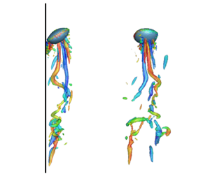
We also conduct simulations of a rising air bubble in stagnant water to examine how many grid points should be located per bubble such that bubble dynamics is correctly represented. We choose the largest bubble ( $d_{eq}=4.16$ mm) among those considered in the present study for these simulations. The grid resolutions tested for the Navier–Stokes and level-set equations are
  $(d_{eq}/\Delta x_{NS},d_{eq}/\Delta x_{LS}) = (8, 16), (16, 32), (24, 48)$ and (32, 64), respectively. This bubble requires a vertical computational domain size of
  $100d_{eq}$ to obtain a bubble path in equilibrium, which requires too much computational cost. Therefore, we rather use a periodic computational box in all directions with a size of
  $(L_x, L_y, L_z) = (4d_{eq},4d_{eq},20d_{eq})$. With this numerical set-up, the wake behind a bubble affects its trajectory, and thus the bubble trajectory should be different from that obtained in a very large domain size. However, this numerical set-up is sufficient to examine the resolution requirement at a much lower computational cost. Figure 7 shows the trajectories of the rising bubble for different grid resolutions. The bubble trajectory from
  $(d_{eq}/\Delta x_{NS},d_{eq}/\Delta x_{LS}) = (8,16)$ is rectilinear, while others are oscillatory. The onsets of oscillatory trajectories occur at the same vertical position (
 $z/d_{eq} = 5.5$) when the initial bubble location is
  $z/d_{eq}=2$, but the subsequent trajectories are different for different grid resolutions. Due to the use of Cartesian coordinates and the relative position of the bubble to the grid, the same trajectory is not expected even with a larger number of grid points. Although the trajectories are different for different grid resolutions, their characteristics from
  $(d_{eq}/\Delta x_{NS},d_{eq}/\Delta x_{LS}) = (24, 48)$ and
  $(32,64)$ are very similar to each other. For example, their dominant frequencies of oscillation,
  $f_{path} \sqrt {d_{eq}/g}$, obtained from the power spectra of the bubble locations on the projected horizontal plane
  $(x,y)$ are 0.111 and 0.115, respectively, while that from
  $(d_{eq}/\Delta x_{NS},d_{eq}/\Delta x_{LS}) = (16, 32)$ is 0.056. This result suggests that the resolution of
  $(24,48)$ should adequately predict the bubble behaviour in water. Figure 8 shows the temporal variations of vertical and horizontal velocities of the rising bubble for different grid resolutions. As shown,
  $(d_{eq}/\Delta x_{NS},d_{eq}/\Delta x_{LS}) = (8,16)$ provides very different velocities from those from denser resolutions. The results from the grid resolutions of
  $(24,48)$ and
  $(32,64)$ are very similar to each other, and those of
  $(16,32)$ are slightly different in terms of oscillation frequency and amplitude from those of
  $(24,48)$ and
  $(32,64)$. The time-averaged terminal velocities from
  $(d_{eq}/\Delta x_{NS},d_{eq}/\Delta x_{LS}) = (8,16), (16,32), (24,48)$ and
  $(32,64)$ are 1.05, 1.19, 1.21 and
  $1.20 \sqrt {g d_{eq}}$, respectively. Therefore, for the bubble of
  $d_{eq} = 4.16$ mm, grid points of
  $(24,48)$ per bubble for the Navier–Stokes and level-set equations, respectively, are required for describing bubble dynamics, and grid points of
  $(16,32)$ are quite marginal. For a smaller size of bubble, the corresponding bubble Reynolds number becomes smaller and thus fewer grid points may be required. In our main simulations, we locate
  $(d_{eq}/\Delta x_{NS},d_{eq}/\Delta x_{LS}) = (25.2, 50.3)$,
  $(21.1, 42.2)$ and
  $(26.6, 53.2)$ for
  $d_{eq}= 2.62, 3.30$ and 4.16 mm, respectively, according to this resolution study. Cano-Lozano et al. (Reference Cano-Lozano, Martinez-Bazan, Magnaudet and Tchoufag2016) and Innocenti et al. (Reference Innocenti, Jaccod, Popinet and Chibbaro2021) used a volume of fluid (VoF) method to predict the dynamics of a single bubble and bubble swarm in still water at
  $Re_{bub}=O(100)$, respectively, and suggested by rigorously examining the bubble path, wake dynamics and bubble shape that a resolution of
  $d_{eq}/\Delta x_{NS} \approx 100$ should be required. Zhang, Ni & Magnaudet (Reference Zhang, Ni and Magnaudet2021, Reference Zhang, Ni and Magnaudet2022) also used the same method to predict the dynamics of a pair of bubbles rising in line at
  $Re_{bub}=O(10)\unicode{x2013}O(100)$, and indicated that
  $d_{eq}/\Delta x_{NS} =136$ is required in the vicinity of bubbles to resolve the boundary layer and wake. Unlike those studies, we examine the turbulence characteristics of bubbly pipe flow (multiple bubbles interacting with the wall) using a marginal number of grid points, and thus the present resolution may not be sufficient to accurately capture small-scale motions behind the bubbles. Such a rigorous analysis conducted by Cano-Lozano et al. (Reference Cano-Lozano, Martinez-Bazan, Magnaudet and Tchoufag2016), Innocenti et al. (Reference Innocenti, Jaccod, Popinet and Chibbaro2021) and Zhang et al. (Reference Zhang, Ni and Magnaudet2021, Reference Zhang, Ni and Magnaudet2022) could be a formidable task for the present flow.

Figure 7. Trajectories for a rising bubble ( $d_{eq} = 4.16$ mm) in the periodic domain with varying grid spacing: (a) three-dimensional view; (b) top view. Blue,
  $(d_{eq}/\Delta x_{NS},d_{eq}/\Delta x_{LS}) = (8,16)$; black, (16,32); green, (24,48); red, (32,64).

Figure 8. Temporal variations of the vertical and horizontal velocities for a rising bubble ( $d_{eq} = 4.16$ mm) in the periodic domain with varying grid spacing: (a) vertical velocity; (b) horizontal velocity. Blue,
  $(d_{eq}/\Delta x_{NS},d_{eq}/\Delta x_{LS}) = (8,16)$; black, (16,32); green, (24,48); red, (32,64).
3. Turbulence statistics and flow structures
3.1. Turbulence statistics
Figure 9 shows the profiles of the mean bubble volume fraction in the radial direction for five bubbly flows. Note that cases ML, MM and MH have the same  $d_{eq}/D$ (
 $=0.0825$) but different
  $\langle \psi \rangle$ values of 0.75 %, 1.5 % and 3.0 %, respectively, and cases SM, MM and LM have the same
  $\langle \psi \rangle$ (
 $=1.5\,\%$) but different
  $d_{eq}/D$ values of 0.0655, 0.0825 and 0.1040, respectively. Except for case LM, the four other cases exhibit radial bubble distributions with peaks near the wall (called wall-peaking) and nearly flat profiles at the pipe centre region. Half the averaging time (
 $T_{avg}$) in table 1 did not change the statistics near the wall but showed slight changes in the centre region (not shown here). Thus, further time averaging should provide slightly better profiles in the centre region, but requires significant amounts of additional computational time (the same argument is applied to the Reynolds normal stress profiles shown in figure 11). Case LM shows that the bubble distribution increases from the centre to
  $r/R=0.4$ and is nearly uniform at
  $r/R=0.4\unicode{x2013}0.8$, followed by a sharp decrease to the wall. This distribution lies between the wall-peaking and core-peaking bubble distributions. According to Dabiri et al. (Reference Dabiri, Lu and Tryggvason2013), the direction of the lift force on a deformable bubble in wall-bounded upward bubbly flow depends on the magnitude of
  $Eo$: i.e. bubbles move towards the centre for
  $Eo > Eo_c$ (
 ${\approx }2.5$) and to the wall otherwise. As shown in table 1,
  $Eo=2.42$ (slightly smaller than
  $Eo_c$) for case LM, whereas
  $Eo$'s are much smaller than
  $Eo_c$ for the four other cases. Therefore, for case LM, more bubbles move away from the wall but do not reach the centre, whereas most bubbles move towards the wall for the four other cases. For a given
  $\langle \psi \rangle$ (cases SM, MM and LM), more bubbles move to the wall with decreasing
  $d_{eq}$. On the other hand, for a given bubble equivalent diameter (i.e. same
  $Eo$; cases ML, MM and MH),
  $\bar \psi$ monotonically increases at all
  $r$'s with increasing
  $\langle \psi \rangle$.

Figure 9. Profiles of the mean bubble volume fraction in the radial direction. Red curve, case ML ( $d_{eq}/D=0.0825$ and
  $\langle \psi \rangle = 0.75\,\%$); solid black curve, case MM (
 $d_{eq}/D=0.0825$ and
  $\langle \psi \rangle = 1.5\,\%$); blue curve, case MH (
 $d_{eq}/D=0.0825$ and
  $\langle \psi \rangle = 3.0\,\%$); dot-dashed curve, case SM (
 $d_{eq}/D=0.0655$ and
  $\langle \psi \rangle = 1.5\,\%$); dashed curve, case LM (
 $d_{eq}/D=0.1040$ and
  $\langle \psi \rangle = 1.5\,\%$).
Figure 10 shows the profiles of the mean velocities of water and bubbles and relative mean bubble velocity in the radial direction for the single-phase and bubbly flows. Here, the mean water and bubble velocities are obtained as
 $$\begin{gather} \bar u_z (r) = \frac{\displaystyle\int_0^{\rm T} \int_0^{L_z} \int_0^{2{\rm \pi}} (1-\psi) u_z \,{\rm d}\theta\,{\rm d} z \,{\rm d} t}{\displaystyle\int_0^{\rm T} \int_0^{L_z} \int_0^{2{\rm \pi}} (1-\psi)\,{\rm d}\theta\,{\rm d} z\,{\rm d} t}, \end{gather}$$
 $$\begin{gather}\bar{u}_{z,{bub}} (r) =\frac{1}{T} \int^{\rm T}_0 \left\{ \frac{1}{N_{bub}(r,t)} \sum^{N_{bub}(r,t)}_{i=1} \frac{1}{V_{b_i}} \int_{V_{b_i}}{u_z \,{\rm d} V} \right\}{\rm d} t, \end{gather}$$
where  $T$ is the integration time,
  $L_z$ is the axial domain size,
  $N_{bub}(r,t)$ is the number of bubbles whose centres of mass are located at
  $r-0.00625D \leq r_{cm} < r+0.00625D$ at time
  $t$ and
  $V_{b_i}$ is the volume of corresponding bubble
  $i$. The water flows with bubbles have higher mean shear rates near the wall than the single-phase flow because of the buoyant bubbles located close to the wall. As the bubble concentration near the wall increases with increasing
  $\langle \psi \rangle$ (ML to MH) and decreasing
  $d_{eq}$ (LM to SM) (see figure 9), the mean shear rates near and at the wall increase (see also
  $Re_\tau$'s in table 1). On the other hand, the mean water velocities of bubbly flows near the centre are lower than that of the single-phase flow and decrease with increasing
  $\langle \psi \rangle$ and decreasing
  $d_{eq}$ owing to the constant mass flow rate. The magnitudes of the mean bubble velocities are greater than two times those of the mean water velocities, and those near the centre increase with decreasing
  $\langle \psi \rangle$ and increasing
  $d_{eq}$ (a similar observation was made in homogeneous bubbly flows by Riboux et al. (Reference Riboux, Risso and Legendre2010) and Roghair et al. (Reference Roghair, Mercado, Annaland, Kuipers, Sun and Lohse2011)). Hence, the relative mean bubble velocities are always positive for the present flows because
  $\bar {u}_{z,{bub}} > \bar u_z$. At
  $r/R <0.8$, the relative mean bubble velocity is almost constant (indicating negligible wall effect in this radial region), and increases slightly with decreasing
  $\langle \psi \rangle$. However, at
  $r/R>0.8$, the relative mean bubble velocity rapidly decreases because the mean bubble velocity rapidly decreases towards the wall while the mean water velocity there increases due to rising bubbles compared with single-phase flow.

Figure 10. Profiles of the mean water and bubble velocities, and relative mean bubble velocity in the radial direction: (a) mean velocities (water and bubble); (b) relative mean bubble velocity.  $\diamond$, Single phase; red, case ML; solid black, MM; blue, MH; dot-dashed, SM; dashed, LM.
Figure 11(a–c) shows the profiles of the r.m.s. water velocity fluctuations in the radial direction for the single-phase and bubbly flows. The bubbly flows have much higher r.m.s. velocity fluctuations at all radial locations than those of the single-phase flow. The r.m.s. velocity fluctuations increase with increasing  $\langle \psi \rangle$ and
  $d_{eq}$. The behaviours of the r.m.s. velocity fluctuations near the centre are similar to those of the mean bubble volume fraction at each radial position (see figure 9): i.e. the magnitudes increase from
  $r/R = 0$ to 0.4 for case LM but are nearly uniform for the other four cases. This is because the fluctuations induced by bubbles are closely related to the number of bubbles present. The axial r.m.s. velocity fluctuations near the wall also show similar behaviours to those of
  $\bar \psi$, but their peak locations are at
  $r/R \approx 0.97$, while the peak of
  $\bar \psi$ locates at
  $r/R = 0.85\unicode{x2013}0.9$. This phenomenon (i.e. shift of the peak locations) is discussed in detail in § 3.2. The radial and azimuthal r.m.s. velocity fluctuations gradually increase towards the wall as compared to the axial velocity component, because these cross-flow components are affected by the wake behind rising bubbles but the axial component is directly influenced by them. Since
  $\bar \psi$ monotonically increases at all the radial locations with increasing
  $\langle \psi \rangle$ (figure 9), the increases of the r.m.s. velocity fluctuation with
  $\langle \psi \rangle$ can be normalized by introducing
  $\bar \psi$. Figure 11(d) shows the r.m.s. water velocity fluctuations normalized by
  $u_{bulk}$ and
  $\bar {\psi }^{0.4}$ for cases ML, MM and MH (
 $\bar \psi = 0.75, 1.5$ and 3.0, respectively, with the same
  $d_{eq}/D=0.0825$). Here,
  $\bar {\psi }^{0.4}$ comes from the studies of homogeneous bubbly flows (Risso & Ellingsen Reference Risso and Ellingsen2002; Martínez-Mercado, Palacios-Morales & Zenit Reference Martínez-Mercado, Palacios-Morales and Zenit2007; Roig & De Tournemine Reference Roig and De Tournemine2007; Riboux et al. Reference Riboux, Risso and Legendre2010) and laminar bubbly pipe flow (Kim, Lee & Park Reference Kim, Lee and Park2016). With this normalization, the profiles of r.m.s. velocity fluctuations for three cases collapse well among themselves at all the radial locations.

Figure 11. Profiles of the r.m.s. water velocity fluctuations in the radial direction: (a)  $u_{r,rms}$; (b)
  $u_{\theta,rms}$; (c)
  $u_{z,rms}$; (d)
  $u_{i,{rms}}/ (u_{bulk} \bar \psi ^{0.4})$.
  $\diamond$, Single phase; red, case ML; solid black, MM; blue, MH; dot-dashed, SM; dashed, LM. In (d), only the cases ML, MM and MH are shown.
As mentioned in § 1, turbulent bubbly flows contain both shear-induced and bubble-induced turbulence. If the shear-induced and bubble-induced turbulence are assumed to be independent from each other, one may decompose the Reynolds normal stresses  $\overline {u_\alpha ^\prime u_\alpha ^\prime }$ as
 \begin{equation} \overline{u_\alpha^\prime u_\alpha^\prime} = R_{SIT} + R_{BIT}, \end{equation}
where  $R_{SIT}$ and
  $R_{BIT}$ denote the Reynolds normal stresses from the shear-induced and bubble-induced turbulence, respectively. Since
  $R_{BIT} \sim \bar \psi ^{0.8}$ (Risso & Ellingsen Reference Risso and Ellingsen2002; Martínez-Mercado et al. Reference Martínez-Mercado, Palacios-Morales and Zenit2007; Roig & De Tournemine Reference Roig and De Tournemine2007; Riboux et al. Reference Riboux, Risso and Legendre2010; Kim et al. Reference Kim, Lee and Park2016), the results in figure 11(d) indicate that the bubble-induced turbulence is predominant even near the wall for the present flows. Note that Lu & Tryggvason (Reference Lu and Tryggvason2008), Dabiri et al. (Reference Dabiri, Lu and Tryggvason2013) and Du Cluzeau et al. (Reference Du Cluzeau, Bois and Toutant2019) indicated the existence of an interaction between the shear-induced and bubble-induced turbulence from their wall-bounded upward bubbly flows. Since their density ratios (
 $\rho _{bubble} / \rho _{liquid}$) considered were about 100 times larger than that of the present study, their bubble-induced turbulence was much weaker than the present one, leading to different conclusions on the effect of the bubble-induced turbulence. The instantaneous flow structures regarding bubble-induced turbulence are discussed later in this paper. In Appendix B, we suggest a modified algebraic RANS model considering the interaction between shear-induced and bubble-induced turbulence for better predictions of the mean axial velocity and wall shear stress for a wider range of liquid bulk Reynolds numbers than those of the previous algebraic RANS model (Sato et al. Reference Sato, Sadatomi and Sekoguchi1981a).
Figure 12 show the probability density functions (PDFs) of the axial velocity fluctuations with normalizations with and without  $\bar \psi ^{0.4}$ at
  $r/R=0.88$ for three different
  $\langle \psi \rangle$. As
  $\langle \psi \rangle$ increases, the peak of PDF normalized by
  $u_{bulk}$ decreases and the PDF becomes widened. On the other hand, when normalized by
  $u_{bulk} \bar \psi ^{0.4}$, the three PDFs collapse quite well as observed from homogeneous bubbly flows (Risso & Ellingsen Reference Risso and Ellingsen2002; Riboux et al. Reference Riboux, Risso and Legendre2010), again indicating that the bubble-induced turbulence is dominant for the present bubbly flows. Similar results are observed for the azimuthal and radial velocities and at other radial locations.

Figure 12. PDFs of the axial water velocity fluctuations at  $r/R=0.88$ normalized by (a)
  $u_{bulk}$ and (b)
  $u_{bulk} \bar {\psi }^{0.4}$: red, case ML; black, MM; blue, MH.
Figure 13 shows the profiles of the water Reynolds shear stress in the radial direction for the single-phase and bubbly flows. The Reynolds shear stress near the wall is much larger due to bubbles than that of the single-phase flow. With increasing  $d_{eq}$ (cases SM, MM and LM), the Reynolds shear stress increases over all the radial locations except very near the centre where
  $\overline {u_r^\prime u_z^\prime }$ is close to zero. On the other hand, with increasing
  $\langle \psi \rangle$ (cases ML, MM and MH), it increases more near the wall but does not change at the centre region (
 $r < 0.5R$). Hence, normalization with
  $\bar \psi ^{0.8}$ works only for the Reynolds normal stresses, not for the Reynolds shear stress, again indicating that the effect of the shear-induced turbulence is very weak for the present flows.

Figure 13. Profiles of the water Reynolds shear stress in the radial direction:  $\diamond$, single phase; red, case ML; solid black, MM; blue, MH; dot-dashed, SM; dashed, LM.
Figure 14 shows the profiles of the body forces in the radial direction for cases SM, MM and LM, together with those of the single-phase flow. The axial RANS equation integrated over the radial direction is
 \begin{equation} \overline{\rho u'_r u'_z}-\overline{\mu \frac{\partial u_z}{\partial r}} =-\frac{r}{2} \varPi -\frac{1}{r} \int^r_0(\bar{\rho}-\langle \rho \rangle) gr\,{\rm d} r +\frac{1}{r} \int^r_0 \sigma \overline{\kappa n_z \delta} r\,{\rm d} r, \end{equation}
where the first and second terms on the left-hand side are the Reynolds and viscous shear stresses, respectively, and the first, second and third terms on the right-hand side are the mean pressure gradient ( $\tau _\beta$), gravitational force (
 $\tau _{grav}$) and surface tension (
 $\tau _{surf}$) terms, respectively. For the single-phase flow, the sum of the Reynolds and viscous shear stresses is proportional to
  $r$. However, for the bubbly flows, it is not linear because of additional gravitational force and surface tension terms that have peaks near the wall. The gravitational force term, which is closely related to the mean bubble volume fraction in that
  $\bar \rho -\langle \rho \rangle = -(\rho _w-\rho _a)(\bar \psi -\langle \psi \rangle )$, significantly changes depending on the bubble equivalent diameter
  $d_{eq}$, while the surface tension term changes relatively little. For case LM, the Reynolds shear stress is much larger at the entire region except near the centre than that of the single-phase flow (figure 13). This is because the gravitational force term is highly positive in the entire region except near the centre and is much larger than the negative surface tension term. As the bubble size gets smaller (from case LM to cases MM and SM), the bubble distribution changes from flat to wall-peaking (see figure 9). Then, the region with
  $\bar \rho (r) > \langle \rho \rangle$ spreads from the centre to the wall, and thus the region with negative
  $\tau _{grav}$ becomes wider. On the other hand,
  $\tau _{surf}$ is negative, especially near the wall (see figure 16( f) for explanation), and does not much change with
  $d_{eq}$. Furthermore, its magnitude near the wall is comparable to that of the mean pressure gradient. Tanaka (Reference Tanaka2011) and Du Cluzeau et al. (Reference Du Cluzeau, Bois and Toutant2019) also numerically observed negative surface tension near the wall, but the underlying reason was not extensively studied. This surface tension term was not taken into account when the profile of
  $\overline {u^\prime _r u^\prime _z}$ was obtained using (3.4) in experimental studies (Wang Reference Wang1986; Colin et al. Reference Colin, Fabre and Kamp2012), as it was challenging to experimentally measure the surface tension. Thus, the Reynolds shear stress profile obtained in those studies matched well the experimental data except near the wall.

Figure 14. Profiles of the body forces in the radial direction: black lines,  $\tau _\beta$; red lines,
  $\tau _{grav}$; blue lines,
  $\tau _{surf}$.
  $\diamond$, Single phase (
 $\tau _\beta$ only); dot-dashed, case SM; solid, MM; dashed, LM.
Equation (3.4) can be used to calculate the mean bubble volume fraction by multiplying this equation by  $r$, differentiating the resulting equation with respect to
  $r$ and introducing
  $\bar \rho -\langle \rho \rangle = -(\rho _w-\rho _a)(\bar \psi -\langle \psi \rangle )$:
 \begin{equation} \bar \psi (r) =\langle \psi \rangle+ \frac{1}{(\rho_w-\rho_a)g} \left\{\frac{1}{r}\frac{\partial}{\partial r} (r\overline{\rho u'_r u'_z})-\frac{1}{r}\frac{\partial}{\partial r} \left(r\overline{\mu \frac{\partial u_z}{\partial r}}\right) + \varPi - \sigma \overline{\kappa n_z \delta}\right\}. \end{equation}
This equation can be also directly obtained from the time-averaged Navier–Stokes equation. Figure 15 shows a comparison of  $\bar \psi$'s from (3.5) with that directly from the present numerical simulations for all the cases considered. As expected, two mean bubble volume fractions calculated as a function of the radial direction agree very well for all the cases.

Figure 15. Comparison of  $\bar \psi$'s (symbols) predicted from (3.5) with those (lines) directly from the present numerical simulations: red and squares, case ML; solid black and squares, case MM; blue and squares, case MH; dot-dashed and circles, case SM; dashed and crosses, case LM.
3.2. Bubble behaviours and instantaneous vortical structures
Figure 16(a–c) shows the bubble trajectories for cases SM, MM and LM. Note that the number of trajectories in each panel is ten and these trajectories are taken at different time instants. Here, the mean major axis length of bubbles  $l_{bub}(r)$ is obtained by calculating the second moment of inertia of the bubbles whose centres of mass are located at
  $r-0.00625D \leq r_{cm} < r+0.00625D$, assuming an ellipsoidal shape, for the purpose of estimating the bubble–wall collision. As shown, when bubbles rise near the wall, they mainly bounce against the wall rather than slide along the wall or hang around the wall without collision. As
  $d_{eq}$ decreases (from LM to SM), more bubbles frequently bounce against the wall. Figure 16(d,e) shows how the mean radial and axial bubble velocities change when bubbles move towards the wall and centre, respectively. Near the wall, the radial velocity for the bubbles moving towards the wall is much higher than that moving towards the centre, while the axial velocities for the bubbles moving to and away from the wall are quite similar to each other. Since a bubble moves in water, its shape is deformed into an ellipsoid such that the direction of the major axis is orthogonal to the bubble movement direction owing to the drag force exerted on the bubble. Thus, near the wall, bubbles moving to the wall are tilted in the clockwise direction, and those moving away from the wall are tilted in the counter-clockwise direction. Since a bubble moving to the wall has stronger radial velocity, the mean bubble shape near the wall is rotated in the clockwise direction. Away from the wall, the radial velocities moving to and away from the wall are nearly the same, and thus the major axis of the mean bubble shape is parallel to the horizontal plane.

Figure 16. Bubble trajectories, conditional mean bubble velocities and mean surface: (a–c) bubble trajectories for cases SM, MM and LM, respectively; (d–e) conditional mean radial and axial bubble velocities ( $\breve u_{r,{bub}}$ and
  $\breve u_{z,{bub}}$), respectively; ( f) surface tension. In (a–c), each trajectory is obtained at a different time, and red dashed lines indicate the locations of
  $r=R-l_{bub}(r)$, where
  $l_{bub}(r)$ is the mean major axis length of bubbles. In (d,e), the red and blue colours denote the mean bubble velocities moving towards the wall and centre, respectively (dot-dashed, case SM; solid, MM; dashed, LM). In ( f), the mean bubble shapes observed at
  $r/R = 0.5$ and 0.89 (case MM) are also shown (their aspect ratios are 1.81 and 1.52, respectively), where red and blue arrows denote the positive and negative axial directions of the surface tension at four locations of the upper and lower bubble surfaces, respectively, and their lengths represent the magnitudes.
Figure 17 shows the mean bubble shapes located at  $r_o/R=0.5$ and 0.89, and surrounding mean streamlines coloured by the contours of the conditionally averaged mean axial velocity for case MM. The mean bubble shapes are reconstructed from their mean vertical angles and lengths of major and minor axes. Their aspect ratios and inclination angles of the minor axis from the vertical direction are
  $AR=$ 1.81 and 1.52 and
  $\theta _i= 0$ and
  $6.08^\circ$, respectively, for the bubbles located at
  $r_o/R = 0.5$ and 0.89. The conditionally averaged mean velocity
  $\tilde {\boldsymbol {u}}$ is obtained by averaging the instantaneous water velocity fields around bubbles located at
  $\vert r-r_o \vert \leq 0.5 \Delta r$. The distribution of the mean streamlines around the bubble located at
  $r_o/R=0.5$ is nearly axisymmetric about the vertical axis (this tendency is observed for the bubbles located at
  $r_o/R<0.8$). On the other hand, the bubble located at
  $r_o/R = 0.89$ and surrounding mean streamlines are asymmetric due to the presence of the wall, as discussed above. When a bubble is located near the wall (figure 17b), the mean streamlines are more asymmetric with respect to the major axis on the wall side than on the centre side (in other words, more acceleration and deceleration of the axial velocity behind and in front of the bubble on its wall side, respectively), which significantly increases the r.m.s. axial velocity fluctuations very near the wall (figure 11c).

Figure 17. Mean shapes of the bubbles located at  $\vert r-r_o \vert \le 0.5 \Delta r$ (
 $\Delta r =0.0039D$), and surrounding mean streamlines coloured by the contours of the conditionally averaged mean axial velocity (case MM): (a)
  $r_o/R=0.5$; (b)
  $r_o/R=0.89$.
The distributions of the mean axial surface tension in the radial direction are shown in figure 16( f) for cases SM, MM and LM, together with schematic diagrams of mean bubble shapes located at  $r_o/R = 0.5$ and 0.89. In the centre region, the axial surface tension is close to zero because the major axis of the mean bubble shape there is nearly perpendicular to the axial direction (like the mean bubble at
  $r_o/R=0.5$) and thus the integral of the surface tension along the bubble surface at each radial location in this region is nearly zero. On the other hand, when the major axis of a bubble is tilted like the mean bubble at
  $r_o/R=0.89$, the curvatures (
 $\kappa$) and angles between the surface-normal and axial directions (
 $\eta = \cos ^{-1}(\vert \boldsymbol {n} \boldsymbol {\cdot } \boldsymbol {k} \vert )$) vary along the bubble surface at each radial location. Then, on the left-hand side (towards the centre) of a bubble, the upper surface has a higher
  $\kappa$ and a smaller
  $\eta$ than the lower surface, resulting in surface tension in the negative axial direction. Likewise, the right-hand side (towards the wall) of a bubble has surface tension in the positive axial direction (see the magnitudes of blue and red arrows on the mean bubble shape at
  $r_o/R=0.89$ in figure 16f). According to this radial distribution of the surface tension (
 $\sigma \overline {\kappa n_z \delta }$), the surface tension term in (3.4), which is the integral of surface tension in the radial direction, is nearly zero in the centre region, negative near the wall, and zero at the wall (see figure 14).
Figure 18 shows the instantaneous vortical structures for the single-phase and bubbly (case MM) flows, coloured by their radial position. Note that a much higher value of  $\vert \lambda _2 \vert$ is used for the bubbly flow because bubble-induced vortices are much stronger than shear-induced vortices. The length scales of these vortices in the bubbly flow are smaller than those in the single-phase flow. It is noteworthy that near-wall coherent structures observed in wall-bounded turbulent flow nearly disappear in the bubbly flow, and most strong vortices are found in the wake behind bubbles. As bubbles are distributed over the whole radial locations (see figure 9), the vortices are observed everywhere in the pipe.

Figure 18. Instantaneous vortical structures identified by the iso-surfaces of  $\lambda _{2}$ (Jeong & Hussain Reference Jeong and Hussain1995) coloured by the radial position: (a) single-phase flow; (b) bubbly flow (case MM). In (b), the bubble surfaces are identified by the iso-surfaces of
  $\psi =0.5$.
Figure 19 shows the instantaneous vortical structures at  $r/R<0.8$, coloured by the contours of the instantaneous axial vorticity for cases SM (
 $d_{eq}/D = 0.0655$ and
  $Re_{bub}=533$), MM (
 $d_{eq}/D = 0.0825$ and
  $Re_{bub}=737$) and LM (
 $d_{eq}/D = 0.1040$ and
  $Re_{bub}=1000$). Note that the region of
  $r/R < 0.8$ is chosen where the relative bubble velocities are nearly uniform (see figure 10b). The vortices behind each bubble in figure 19 are qualitatively similar to those behind a freely rising air bubble at a similar
  $Re_{bub}$ (Brücker Reference Brücker1999; De Vries, Biesheuvel & Van Wijngaarden Reference De Vries, Biesheuvel and Van Wijngaarden2002). For case SM (figure 19a), the wake behind a bubble consists of double-threaded vortices (denoted as a dashed ellipse) that primarily convey the axial vorticity. For case MM (figure 19b), the wake consists of not only double-threaded vortices but also hairpin vortices (shown below panel (b)) that carry the horizontal vorticity components as well as the axial one. Symmetric hairpin vortices are often observed in the wake of a single bubble rising in a zigzag trajectory (Brücker Reference Brücker1999). For the present flow, hairpin vortices in the wake of bubbles are predominantly one-sided (i.e. one-legged) rather than symmetric (two-legged) because of complex interactions among bubbles and their wake. For case LM (figure 19c), the wake contains a bunch of double-threaded and hairpin vortices. These vortices are denser and more irregular than those observed from case MM. A toroidal vortex is also observed inside bubble surfaces (denoted as a solid curve in figure 19a) for all the cases considered (see below for details).

Figure 19. Instantaneous vortical structures (identified by  $\lambda = - 400$) at
  $r/R<0.8$ coloured by the contours of the instantaneous axial vorticity
  $\omega _{z}$: (a)
  $d_{eq}/D=0.0655$ (SM); (b)
  $d_{eq}/D=0.0825$ (MM); (c)
  $d_{eq}/D=0.1040$ (LM). Here, the bubble surfaces are identified by the iso-surfaces of
  $\psi =0.5$. Thick solid and dashed ellipses in (a) indicate toroidal and double-threaded vortices, respectively. Below (b), one-sided hairpin vortices (‘A’ and ‘B’) in the wake of a bubble are identified for case MM.
Figure 20 shows the instantaneous wall shear stress for the single-phase and bubbly flows (cases SM, MM and LM). Note that the mean wall shear stresses of cases SM, MM and LM are 3.22, 2.51 and 2.02 times that of the single-phase flow, respectively (table 1). The streaky structure of the wall shear stress observed for the single-phase flow does not exist, but spotty structures are found in the bubbly flows. As  $d_{eq}$ increases, the spotty structure occurs less frequently but increases in size.

Figure 20. Contours of the instantaneous wall shear stress: (a) single-phase flow; (b) case SM; (c) MM; (d) LM.
Figure 21 shows the time sequence of a bubble near the wall and associated vortices for case MM, together with the contours of the wall shear stress beneath the bubble. At  $tu_{bulk}/D=16.35$, a bubble approaches the wall, and negative wall shear stress occurs behind the bubble. When a bubble moves upward and approaches the wall, an inclined stagnation flow is generated beneath the bubble, and a reverse flow region is formed just under the bubble, as shown in figure 22, resulting in a negative wall shear stress region there. Note also that a toroidal vortex is generated inside the bubble and the direction of rotation of this vortex near the wall is same as that of the velocity field under the bubble (see figure 22). During wall–bubble collision (
 $tu_{bulk}/D=16.40$), regions of high wall shear stress occur beneath and behind the bubble owing to its sweeping motion towards the wall and the wall-ward velocity induced by a pair of counter-rotating vortices behind the bubble, respectively. This pair of vortices are generated by the interaction of the bubble with the wall (see these vortices very near the wall from
  $(z,r)$ plane view at
  $tu_{bulk}/D=16.40$). This pair of vortices further develops as the bubble bounces off the wall and creates a region of longer high wall shear stress (
 $tu_{bulk}/D=16.50$). Note that, at this instant, the signs of counter-rotating vortices are opposite to those at
  $tu_{bulk}/D=16.35$ (this is very different from those of bouncing counter-rotating vortices behind a bubble in still water (Lee & Park Reference Lee and Park2017)), and the velocity induced by these vortices in the wake pushes the bubble away from the wall. However, at
  $tu_{bulk}/D=16.70$, the bubble moves towards the wall again by the high shear near the wall, and generates a new pair of near-wall counter-rotating vortices right behind the bubble, resulting in high skin friction there. Note that a pair of long counter-rotating vortices behind the bubble are generated from the wall-ward motion of the bubble and has opposite signs of rotation to those generated from the interaction with the wall. Also, the region of the high wall shear stress and near-wall vortices created during
  $tu_{bulk}/D=16.40\unicode{x2013}16.50$ persist at
  $tu_{bulk}/D=16.70$, although the corresponding bubble moves away from these flow structures. These vortical structures near the wall significantly increase the mean skin friction and r.m.s. velocity fluctuations very near the wall (figure 11). Lu & Tryggvason (Reference Lu and Tryggvason2008, Reference Lu and Tryggvason2013) numerically observed for a density ratio of
  $\rho _{bubble}/\rho _{liquid} = 0.1$ that most bubbles slide along the channel walls and form a cluster for wall-peaking turbulent bubbly channel flows. This difference in bubble–wall interactions may come from very different density ratios considered. Figure 23 shows the instantaneous vortical structure around bouncing-off bubbles for cases SM, MM and LM. As
  $d_{eq}$ increases, the vortices generated by the interaction of the bubble with the wall become stronger and more complex. Nevertheless, the most important vortices are the pair of counter-rotating vortices that induce high-speed water flow towards the wall and create high wall shear stress, as discussed in figure 21.

Figure 21. Time sequence of a bubble near the wall and associated vortices coloured by the contours of the instantaneous axial vorticity, and contours of the instantaneous wall shear stress beneath the bubble (case MM): (a) (left)  $(z,r)$ and (right)
  $(z,\theta )$ plane views; (b) wall shear stress. Here, the bubble surfaces are identified by the iso-surfaces of
  $\psi =0.5$. In (a), red arrows represent the instantaneous bubble velocities. In (b), dotted circles indicate the locations of the bubble projected on the wall.

Figure 22. A bubble approaching wall and nearby velocity field, together with a toroidal vortex inside the bubble at  $tu_{bulk}/D=16.35$ (case MM): (a) top view; (b) side view. Here, the bubble surface (thin black circle) and toroidal vortex (green colour) are identified by the iso-surfaces of
  $\psi =0.5$ and
  $\lambda _2 = -1875$, respectively.

Figure 23. Instantaneous vortical structures (identified by  $\lambda = - 400$) behind a bouncing-off bubble coloured by the contours of the instantaneous axial vorticity
  $\omega _{z}$: (a)
  $d_{eq}/D=0.0655$ (case SM); (b)
  $d_{eq}/D=0.0825$ (case MM); (c)
  $d_{eq}/D=0.1040$ (case LM). Here, the bubble surfaces are identified by the iso-surfaces of
  $\psi =0.5$. The bubble radial locations are
  $r_o=0.855, 0.845$ and
  $0.849R$ for cases SM, MM and LM, respectively.
Figure 24 shows the PDFs of the directional angle ( $\alpha$) of the bubble velocity vector deviated from the axial direction for the bubbles located at
  $0.45< r/R<0.50$ and
  $0.85< r/R<0.90$ (cases ML, MM and MH). Here, the PDF is obtained as
  ${\rm PDF} (\alpha _o, \theta _o) = N(\vert \alpha - \alpha _o \vert \le \Delta \alpha /2,\ \vert \theta - \theta _o \vert \le \Delta \theta / 2) / \{N(0^\circ \le \alpha \le 180^\circ, 0^\circ \le \theta \le 360^\circ ) \times \sin \alpha \Delta \alpha \Delta \theta \}$, where
  $N(\,{\cdot}\,)$ is the number of events,
  $\Delta \alpha = 1.41^\circ$ and
  $\Delta \theta = 5.63^\circ$. No bubble is observed to move downward, and thus the directional angles of
  $0^\circ \le \alpha \le 90^\circ$ are drawn in this figure. When bubbles move homogeneously in
  $0^\circ \le \alpha \le 90^\circ$, the magnitude of the PDF is constant (
 $=1/(2{\rm \pi} )=0.159$). For the bubbles located at
  $0.45< r/R<0.50$ (top panels in figure 24a–c), the contours of the PDF are nearly axisymmetric, indicating that there is no preferred horizontal movement direction and bubbles located away from the wall are little affected by the pipe wall. However, the PDFs have clear peaks at
  $\alpha \approx 16^\circ, 14^\circ$ and
  $10^\circ$ for cases ML, MM and MH, respectively. That is, as
  $\langle \psi \rangle$ increases, more bubbles located at
  $0.45< r/R<0.50$ move at a smaller directional angle from the vertical direction, and the PDF at
  $\alpha =0^\circ$ increases. Now, let us consider the bubbles located at
  $0.85< r/R<0.90$ where
  $\bar \psi$ is high (figure 9). At this radial location (bottom panels in figure 24a–c), the contours of the PDF are asymmetric and inclined towards the pipe centre. The most preferred directional angles are
  $\alpha \approx 9^\circ, 8^\circ$ and
  $7^\circ$ towards the pipe centre for cases ML, MM and MH, respectively. Note also that there are clear second peaks of the PDF (arc-shaped contours in this figure) at
  $\alpha \approx 19^\circ, 17^\circ$ and
  $13^\circ$ towards the wall region for cases ML, MM and MH, indicating that the wall-approaching angle of bubbles is statistically larger than the bounce-off angle.

Figure 24. PDFs of the directional angle of the bubble velocity vector deviated from the axial direction for the bubbles located at  ${0.45< r/R<0.50}$ (top) and
  $0.85< r/R<0.90$ (bottom): (a) case ML; (b) MM; (c) MH. Here, ‘c’ and ‘w’ denote the directions towards the pipe centre and wall from a bubble location, respectively.
4. Conclusions
In the present study, we investigated the turbulence characteristics, bubble behaviour and vortical structures in an air–water upward bubbly pipe flow at  $Re_{bulk}=5300$ and
  $Re_{bub}=533\unicode{x2013}1000$ using a high-resolution numerical simulation. A single-phase flow and five monodispersed bubbly flows with varying bubble equivalent diameter (
 $d_{eq} = 2.62, 3.30, 4.16$ mm) and total bubble volume fraction (
 $\langle \bar {\psi } \rangle = 0.75\,\%, 1.5\,\%, 3.0\,\%$) were examined. Flat and wall-peaking bubble distributions were observed, respectively, for the case with the largest
  $d_{eq}$ (
 $=4.16$ mm) and the other four cases. These radial bubble distributions significantly affected the turbulence statistics of bubbly flows.
As the bubble concentration near the wall increased with increasing total bubble volume rate and decreasing bubble equivalent diameter, the mean shear rates near and at the wall increased significantly. The profiles of the r.m.s. velocity fluctuations of the bubbly flows were proportional to  $\bar {\psi }^{0.4}$ (
 $\bar \psi (r)$ is the mean bubble volume fraction), which is a characteristic of bubble-induced turbulence as observed for homogeneous bubbly flows by Risso & Ellingsen (Reference Risso and Ellingsen2002) and Riboux et al. (Reference Riboux, Risso and Legendre2010). This result indicated that shear-induced turbulence was suppressed in the present bubbly flows. The vortices in the bubbly flows were smaller in size but denser and more intense than those in the single-phase flow. Consequently, the bubble-induced vortices were strong enough to hinder the development of shear-induced vortices, and the velocity fluctuations primarily exhibited the characteristics of bubble-induced turbulence. The Reynolds shear stress was analysed considering the balance among the viscous shear stress, mean pressure gradient, gravitational force and surface tension in the Reynolds-averaged axial momentum equation. The Reynolds shear stress around the pipe centre mainly came from the positive mean pressure gradient and negative gravitational force, while those near the wall came from the positive gravitational force and negative surface tension in addition to the positive mean pressure gradient. The positive and negative peaks of the surface tension near the wall were caused by the stronger bubble motion towards the wall and tilted bubble shape. Bubbles near the wall approached and bounced off the wall. After collision with the wall, counter-rotating vortices in the wake of bubbles were generated and increased the skin friction. As the bubble equivalent diameter increased, they became more tilted and complicated, and induced higher water velocity to the wall.
We suggested a modified algebraic RANS model based on the interaction between shear-induced and bubble-induced turbulence. Unlike the previous RANS model of Sato et al. (Reference Sato, Sadatomi and Sekoguchi1981a), the present one considered relative strengths of these types of turbulence. The present model showed a better performance than the previous one at a wide range of the water bulk Reynolds number.
Funding
This work was supported by the National Research Foundation of Korea (nos. 2017M2A84018482 and 2021R1A4A1032023). The computer resources were provided by the KISTI Super Computing Center (no. KSC-2020-CRE-0228).
Declaration of interests
The authors report no conflict of interest.
Appendix A. Numerical methods
Equations (2.1) and (2.2) are solved using a semi-implicit four-step fractional-step method:
 \begin{gather} \frac{\hat{\rho}-\rho^{k-1}}{2 \alpha_k \Delta t}=-\frac{\beta_k}{2 \alpha_k} \boldsymbol{\nabla}\boldsymbol{\cdot} (\rho^{k-1}_f \boldsymbol{u}^{k-1}) -\frac{\gamma_k}{2 \alpha_k} \boldsymbol{\nabla}\boldsymbol{\cdot} (\rho^{k-2}_f \boldsymbol{u}^{k-2}), \end{gather}
 \begin{gather} \begin{aligned}\frac{\hat{\rho} \hat{\boldsymbol{u}}-\rho^{k-1} \boldsymbol{u}^{k-1}}{2 \alpha_k \Delta t} &=- \varPi^{k-1} \boldsymbol{k}- \boldsymbol{\nabla} p^{k-1} +\frac{1}{2} \{\boldsymbol{L} ({\hat{\mu}}, \hat{\boldsymbol{u}}) + \boldsymbol{L} (\mu^{k-1}, \boldsymbol{u}^{k-1})\} \nonumber\\ &\quad +\frac{\beta_k}{2 \alpha_k} \boldsymbol{N} (\rho^{k-1}_f, \mu^{k-1}, \boldsymbol{u}^{k-1}) +\dfrac{\gamma_k}{2 \alpha_k} \boldsymbol{N} (\rho^{k-2}_f, \mu^{k-2}, \boldsymbol{u}^{k-2}) \nonumber\\ &\quad +\left\{\frac{1}{2}(\hat{\rho}+\rho^{k-1})-\langle \rho \rangle\right\} \boldsymbol{g} +\sigma \kappa^{k-1} \delta^{k-1} \boldsymbol{n}^{k-1}+\boldsymbol{f}^k,\end{aligned} \end{gather}
 $$\begin{gather} \frac{\hat{\rho} \boldsymbol{u}^*-\hat{\rho} \hat{\boldsymbol{u}}}{2 \alpha_k \Delta t}= \varPi^{k-1} \boldsymbol{k} + \boldsymbol{\nabla} p^{k-1}, \end{gather}$$
 $$\begin{gather}\boldsymbol{\nabla}\boldsymbol{\cdot} \left(\frac{1}{\hat{\rho}} (\varPi^k \boldsymbol{k} + \boldsymbol{\nabla}p^k)\right)= \frac{1}{2\alpha_k \Delta t} \boldsymbol{\nabla} \boldsymbol{\cdot} \boldsymbol{u}^*, \end{gather}$$
 $$\begin{gather}\frac{\hat{\rho} \boldsymbol{u}^k-\hat{\rho} \boldsymbol{u}^*}{2 \alpha_k \Delta t}=- \varPi^k \boldsymbol{k} -\boldsymbol{\nabla} p^k, \end{gather}$$
where
 $$\begin{gather} \boldsymbol{L}(\mu,\boldsymbol{u})=\boldsymbol{\nabla} \boldsymbol{\cdot} (\mu \boldsymbol{\nabla} \boldsymbol{u})+ \boldsymbol{\nabla}\boldsymbol{\cdot} \boldsymbol{D}(\mu \boldsymbol{\nabla}^{\rm T} \boldsymbol{u}), \end{gather}$$
 $$\begin{gather}\boldsymbol{N}(\rho,\mu,\boldsymbol{u})=-\boldsymbol{\nabla}\boldsymbol{\cdot} (\rho \boldsymbol{u} \boldsymbol{u})+\boldsymbol{\nabla}\boldsymbol{\cdot} \boldsymbol{ND}(\mu \boldsymbol{\nabla}^{\rm T} \boldsymbol{u}), \end{gather}$$
 $\hat {\rho }$ is the provisional density obtained by (A1),
  $\rho _f$ (
 $=\rho _a \psi _{\varGamma }+ \rho _w (1-\psi _{\varGamma })$) is an upwind-type flux density defined at a cell face,
  $\psi _{\varGamma }$ is the bubble volume fraction of the region
  ${\varGamma }$ that contains fluids passing through the cell face during
  $\beta _k \Delta t$ at
  $t=t^{k-1}$ (for
  $\rho ^{k-1}_f$) or
  $\gamma _k \Delta t$ at
  $t=t^{k-2}$ (for
  $\rho ^{k-2}_f$),
  $\hat {\mu }$ is the viscosity calculated from (2.4) with
  $\hat {\rho }$ and
  $\psi$ obtained by (A1) and (2.3), respectively,
  $\hat {\boldsymbol {u}}$ and
  $\boldsymbol {u}^{*}$ are the intermediate velocities,
  $\boldsymbol {D}(\boldsymbol {T} )$ and
  $\boldsymbol {ND}(\boldsymbol {T} )$ are the tensors consisting of diagonal and non-diagonal elements of tensor
  $\boldsymbol {T}$, respectively, and the subscript
  $k$ (
$k$ ( $=1,2,3$) is the sub-time-step index (
 $\alpha _{1}=4/15$,
  $\alpha _{2}=1/15$,
  $\alpha _{3}=1/6$,
  $\beta _{1}=8/15$,
  $\beta _{2}=5/12$,
  $\beta _{3}=3/4$,
  $\gamma _{1}=0$,
  $\gamma _{2}=-17/60$,
  $\gamma _{3}=-5/12$). Here, a third-order Runge–Kutta method is applied to the convection and non-diagonal viscous terms, and the Crank–Nicolson method is applied to the viscous (excluding non-diagonal term) and gravitational terms. An explicit Euler method is used for the surface tension term to achieve a discrete balance between the surface tension and pressure gradient forces (Kim Reference Kim2011). The second-order central difference method is used for all spatial derivative terms except for the convection terms at the phase interface cell in (A1) and (A2) where an upwind-type mass-flux method (Kim Reference Kim2011; Kim & Choi Reference Kim and Choi2018) is used. These consistent temporal and spatial discretization methods adopted for the convection terms in (A1) and (A2) ensure an accurate momentum transport, which is crucial for the present simulation of two-phase flow with a high density ratio (
 $\rho _w/\rho _a \approx 1000$) (Raessi & Pitsch Reference Raessi and Pitsch2012).
A multigrid preconditioned conjugate gradient method (Tatebe Reference Tatebe1993) is used to solve the variable-coefficient Poisson equation (A4). Approximately 20 iterations are needed to satisfy a convergence criterion of  $\vert \boldsymbol {\nabla }\boldsymbol {\cdot } \boldsymbol {u}\vert _{max} < 10^{-6}$, which consumes approximately 40 % of the whole computational time. The size of the computational time step is restricted by the conventional Courant–Friedrichs–Lewy (CFL) condition on the convective term (CFL
 $_{max} \le \sqrt {3}$) and also by the capillary time-step constraint induced by the explicit treatment of the surface tension term (Brackbill, Kothe & Zemach Reference Brackbill, Kothe and Zemach1992):
 \begin{equation} \Delta t \leq \sqrt{\frac{(\rho_a+\rho_w) \Delta x^3_{min}}{4{\rm \pi}\sigma}}, \end{equation}
where  $\Delta x_{min}$ is the smallest grid size. For the present problem, the computational time step is mostly bounded by (A8).
Equation (2.5) is solved using a third-order total variation diminishing (TVD) Runge–Kutta method (Gottlieb & Shu Reference Gottlieb and Shu1998) and a fifth-order weighted essentially non-oscillatory (WENO) scheme in conjunction with a local Lax–Friedrichs entropy correction (Jiang & Peng Reference Jiang and Peng2000) for temporal and spatial discretizations, respectively. To maintain the signed-distance property, the level-set function is reinitialized at every other time step by solving the following partial differential equation (Sussman, Smereka & Osher Reference Sussman, Smereka and Osher1994; Peng et al. Reference Peng, Merriman, Osher, Zhao and Kang1999):
 \begin{equation} \frac{\partial \phi}{\partial \tau_r}+\frac{\phi}{\sqrt{\phi^2+\vert \boldsymbol{\nabla} \phi \vert^2 \Delta x^2_\phi}} (\vert \boldsymbol{\nabla} \phi \vert -1)=0, \end{equation}
where  $\tau _r$ is the pseudo-time for the reinitialization iteration and
  $\Delta x_\phi$ is the level-set grid size. Equation (A9) is iteratively solved using a third-order TVD Runge–Kutta method in time and a fifth-order WENO scheme with a Godunov flux scheme in space. The volume of each bubble is conserved by relocating the phase interface from
 \begin{equation} \frac{\partial \phi}{\partial \tau_v}=\frac{\phi}{\sqrt{\phi^2+\vert \boldsymbol{\nabla} \phi \vert^2 \Delta x^2_\phi}} \frac{V_b(t)-V_b(t=0)}{V_b(t=0)}, \end{equation}
where  $\tau _v$ is the pseudo-time for the volume correction iteration and
  $V_b$ is the bubble volume (Son Reference Son2001; Zhang et al. Reference Zhang, Zou, Greaves, Reeve, Hunt-Raby, Graham, James and Lv2010). We assign a level-set function to each bubble to avoid numerical coalescence (Coyajee & Boersma Reference Coyajee and Boersma2009). Each level-set function is solved in the cuboid which contains a bubble and at least six grid points outside the bubble interface. When a bubble locates very near the pipe wall, only the level-set grid points located inside the pipe are used to solve (2.5). If a bubble penetrates the pipe wall, a special treatment is required. However, this did not occur at all (because of the velocity distribution very near the wall) during
  $tu_{bulk}/D = 10$ for all cases considered, and thus such a treatment was not needed.
According to Sanada et al. (Reference Sanada, Sato, Shirota and Watanabe2009), bubbles in water coalesce at  $Re_{bub} < 540\unicode{x2013}590$. Among the cases considered, the bubble Reynolds number of case SM (
 $Re_{bub} = 533$ and
  $d_{eq}=2.62$ mm; see table 1) is within this criterion. However, the bubble volume fraction of case SM is only
  $\langle \psi \rangle = 1.5\,\%$ and thus the possibility of bubble collisions must be very low. Riboux et al. (Reference Riboux, Risso and Legendre2010) also indicated that bubble coalescence was not observed in a homogeneous bubbly flow for
  $d_{eq} = 1.6, 2.1$ and 2.5 mm and
  $\langle \psi \rangle = 0.5\,\%\unicode{x2013}10\,\%$. Therefore, for all the cases considered in the present study, we expect that bubble coalescence does not occur or little affects the flow fields even if it happens.
When bubbles approach very closely to the wall and rebound from the wall, a thin liquid film is formed and thus resolving this thin film is required. Typically, the number of grid points within this liquid film (for the Navier–Stokes equations) can reach one or two during simulation. Nevertheless, the time period of having one or two grids within thin film is very short ( $tu_{bulk}/D \approx 0.03$) because of the upward water flow and repulsive force from the wall, and thus numerical errors may not be noticeably accumulated during bubble–wall interactions. Albadawi et al. (Reference Albadawi, Donoghue, Robinson, Murray and Delauré2014) conducted numerical simulations for a bouncing bubble from a horizontal surface with and without mesh refinement near the wall. The results with mesh refinement (having a mesh size smaller than liquid film thickness) were better than those without mesh refinement (mesh size was about 50 times that of refined mesh). However, the simulation without mesh refinement still captured the temporal variation of the bubble velocity during four rebounding periods. The use of adaptive mesh reported recently (Innocenti et al. Reference Innocenti, Jaccod, Popinet and Chibbaro2021; Yan et al. Reference Yan, Zhang, Liao, Zhang, Zhou and Liu2022) will further improve the numerical accuracy during this time period.
Appendix B. A modified algebraic RANS model
In this appendix, we revisit the algebraic model by Sato et al. (Reference Sato, Sadatomi and Sekoguchi1981a) for the predictions of the wall shear stress and mean axial velocity profile, and suggest a revised model by introducing the effect of the interaction between the shear-induced and bubble-induced turbulence.
Sato et al. (Reference Sato, Sadatomi and Sekoguchi1981a) provided the following equation for the mean velocity gradient in a pipe assuming that the dispersed gas phase is void:
 \begin{equation} \frac{{\rm d} \bar{u}_z}{{\rm d} r}=\frac{1}{\rho_w(1-\bar{\psi})(\nu_w+\nu_t)} \left\{\frac{r}{R} \left(-\tau_{w}+ \frac{\rho_w g}{R} \int_0^R{\bar{\psi}r\,{\rm d} r}\right)- \frac{\rho_w g}{r} \int_0^r{\bar{\psi}r\,{\rm d} r}\right\}, \end{equation}
with
 $$\begin{gather} \nu_t (r) =\nu_{SIT} (r) +\nu_{BIT} (r), \end{gather}$$
 $$\begin{gather}\nu_{SIT} (r) =k_0 \nu_w C_r \left\{1-\frac{11}{6} \left(\frac{R-r}{R}\right) +\frac{4}{3} \left(\frac{R-r}{R} \right)^2 -\frac{1}{3} \left(\frac{R-r}{R}\right)^3\right\} (R^+-r^+), \end{gather}$$
 $$\begin{gather}\nu_{BIT}(r)=\frac{1}{2} k_1 C_r \hat{d}_{eq} \bar{\psi} (u_{bub}-u_{bulk}) \approx \frac{1}{2} k_1 C_r \hat{d}_{eq} \bar{\psi} u_T, \end{gather}$$
where  $\nu _w$ is the water kinematic viscosity,
  $\nu _t$ is the turbulent kinematic viscosity decomposed into the shear-induced (
 $\nu _{SIT}$) and bubble-induced (
 $\nu _{BIT}$) kinematic viscosities,
  $C_r=(1-\exp {(-(R^+-r^+)/A^+)})^2$,
  $r^+=r u_\tau /\nu _w$,
  $R^+=R u_\tau /\nu _w$,
  $u_\tau =\sqrt {\tau _w/\rho _w}$,
  $A^+$ (
 $=16$) is the van Driest (Reference van Driest1956) damping factor coefficient,
  $k_0$ (
 $=0.4$) and
  $k_1$ (
 $=1.2$) are empirical constants and
  $\hat {d}_{eq} = d_{eq}$ for
  $0 \le r < R-d_{eq}/2$ and
  $4(R-r)(d_{eq}-(R-r))/d_{eq}$ for
  $R-d_{eq}/2 \le r \le R$. Since the relative bubble velocity,
  $u_{bub}-u_{bulk}$, in (B4) is unknown a priori, the mean terminal velocity of rising bubbles (
 $u_T$) was used instead of
  $u_{bub}-u_{bulk}$. For the present computations, we obtain
  $u_T$ from the plot of
  $d_{eq}$ versus
  $u_T$ in Clift, Grace & Weber (Reference Clift, Grace and Weber2005). Note that
  $\nu _{SIT}$ in (B3) is based on single-phase turbulent pipe flow. Also, the radial distribution of
  $\bar \psi (r)$ has to be given a priori to solve (B1).
In §§ 3.1 and 3.2, we observed that bubble-induced turbulence hinders the development of shear-induced turbulence when the vorticity magnitude of bubble-induced turbulence is much larger than that of shear-induced turbulence (see figures 18 and 11). However, the model suggested by Sato et al. (Reference Sato, Sadatomi and Sekoguchi1981a) contains both characteristics irrespective of the relative strength of both turbulence types. Therefore, the turbulent kinematic viscosity is modified by introducing  $\chi$ as follows:
 \begin{equation} \nu_t(r) =(1-\chi) \nu_{SIT}(r) +\chi \nu_{BIT}(r), \end{equation}
with
 \begin{equation} \chi = \exp{(-k_2 u_{bulk}/(u_{bub}-u_{bulk}))} \approx \exp{(-k_2 u_{bulk}/u_T)}, \end{equation}
where  $\chi$ is the fraction of bubble-induced turbulence
  $(0 \le \chi \le 1)$. The empirical constants
  $k_1$ and
  $k_2$ in (B4) and (B6) are determined by an iterative method such that the predicted wall shear stresses match those of case 2 (from present simulation) and case 14 (from an experiment by Liu (Reference Liu1997)). These two cases correspond to the smallest and largest water bulk velocities investigated in the present study, respectively (see table 4). As a result, we obtain
  $k_1=13.1$ and
  $k_2=0.359$, and use them for the prediction. We note that there may be a better representation of
  $\chi$ by introducing more variables such as
  $R/d_{eq}$,
  $Re_{bub}$,
  $Re_{bulk}$, etc. However, we do not pursue this issue further because the present definition of
  $\chi$ can successfully predict the wall shear stress for the cases considered.
Table 3 shows the computational procedure to obtain the mean axial velocity and wall shear stress using the present algebraic RANS model. The number of grid points in the radial direction is 201, where the smallest and largest grid spacings are  $\Delta r/R = 0.001$ at the wall (
 $r=R$) and 0.028 at the centre (
 $r=0$), respectively. We use the trapezoidal method for numerical integrations in Steps 4 and 5. Term
  $\mathcal {D}u_{bulk}/{\mathcal {D}\tau _w}$ in Step 6 is obtained as follows. From (B1) together with
  $u_{bulk}=2\int ^R_0{\bar {u}_z(r)r\,{\rm d} r}/R^2$, one can express
  $u_{bulk}$ as a function of
  $\tau _w$:
 \begin{align} u_{bulk}(\tau_w) &=-\frac{2\tau_w}{\rho_w R^3} \int_0^R{r\int_R^r{\frac{r'}{(1-\bar{\psi}(r'))(\nu_w+\nu_t(\tau_w,r'))}{\rm d} r'}\,{\rm d} r} \nonumber\\ &\quad +\frac{2g}{R^4}\int_0^R{\bar{\psi}(r'')r''\,{\rm d} r''} \int_0^R{r\int_R^r{\frac{r'}{(1-\bar{\psi}(r'))(\nu_w+\nu_t(\tau_w,r'))}{\rm d} r'}\,{\rm d} r} \nonumber\\ &\quad -\frac{2g}{R^2}\int_0^R{r\int_R^r{\frac{1}{r'(1-\bar{\psi}(r'))(\nu_w+\nu_t(\tau_w,r'))} \int_0^{r'}{\bar{\psi}(r'')r''\,{\rm d} r''}\,{\rm d} r'}\,{\rm d} r}. \end{align}
By taking the derivative of (B7) with respect to  $\tau _w$, we obtain
  $\mathcal {D}u_{bulk}/{\mathcal {D}\tau _w}$ as follows:
 \begin{align} \frac{\mathcal{D}u_{bulk}}{\mathcal{D}\tau_w} &=-\frac{2}{\rho_w R^3}\int_0^R{r\int_R^r{\frac{r'}{(1-\bar{\psi}(r'))(\nu_w+\nu_t(\tau_w,r'))}\,{\rm d} r'}\,{\rm d} r} \nonumber\\ &\quad +\frac{2\tau_w}{\rho_w R^3}\int_0^R{r\int_R^r{\frac{r'\mathcal{D} \nu_t(\tau_w,r')/\mathcal{D}\tau_w}{(1-\bar{\psi}(r'))(\nu_w+\nu_t(\tau_w,r'))^2}\,{\rm d} r'}\,{\rm d} r} \nonumber\\ &\quad -\frac{2g}{R^4}\int_0^R{\bar{\psi}(r'')r''\,{\rm d} r''} \int_0^R{r\int_R^r{\frac{r'\mathcal{D}\nu_t(\tau_w,r')/\mathcal{D}\tau_w}{(1-\bar{\psi}(r')) (\nu_w+\nu_t(\tau_w,r'))^2}{\rm d} r'}\,{\rm d} r} \nonumber\\ &\quad +\frac{2g}{R^2}\int_0^R{r\int_R^r{\frac{\mathcal{D}\nu_t(\tau_w,r')/\mathcal{D} \tau_w}{r'(1-\bar{\psi}(r'))(\nu_w+\nu_t(\tau_w,r'))^2} \int_0^{r'}{\bar{\psi}(r'')r''\,{\rm d} r''}\,{\rm d} r'}\,{\rm d} r}, \end{align}
where  $\mathcal {D}\nu _t(\tau _w,r')/\mathcal {D}\tau _w$ is obtained from (B5) as
 \begin{align} \frac{\mathcal{D}\nu_t(\tau_w,r')}{\mathcal{D}\tau_w} &= (1-\chi) \frac{\mathcal{D}\nu_{SIT}(\tau_w,r')}{\mathcal{D}\tau_w}+\chi \frac{\mathcal{D}\nu_{BIT}(\tau_w,r')}{\mathcal{D}\tau_w} \nonumber\\ &= (1-\chi)\left\{ \frac{1}{2}+\frac{R^+-r'^+}{A^+} \frac{\exp(-(R^+-r'^+)/A^+)}{(1-\exp(-(R^+-r'^+)/A^+)}\right\} \frac{\nu_{SIT}(\tau_w,r')}{\tau_w} \nonumber\\ &\quad +\chi \left\{\frac{R^+-r'^+}{A^+}\frac{\exp(-(R^+-r'^+)/A^+)}{(1-\exp(-(R^+-r'^+)/A^+)}\right\} \frac{\nu_{BIT}(\tau_w,r')}{\tau_w}. \end{align}
Table 3. Iterative method to calculate the wall shear stress and mean axial velocity profile using the present RANS model. Here,  $l$ (
$l$ ( $=1,2,3,\ldots$) is the iteration index.

Table 4 shows the cases considered by the present simulation, Inoue et al. (Reference Inoue, Aoki, Koga and Yaegashi1976), Sato et al. (Reference Sato, Sadatomi and Sekoguchi1981b), Malnes (Reference Malnes1966) and Liu (Reference Liu1997) for testing the present algebraic model. The terminal velocities ( $u_T$) of all the cases are obtained from the plot of
  $d_{eq}$ versus
  $u_T$ for a bubble in pure water in Clift et al. (Reference Clift, Grace and Weber2005), with which the computed
  $\chi$ ranges from 0.024 to 0.838. Figure 25 shows the errors in the wall shear stress predicted by the present model and that of Sato et al. (Reference Sato, Sadatomi and Sekoguchi1981a) for the data available from the present simulation and previous experiments (Malnes Reference Malnes1966; Inoue et al. Reference Inoue, Aoki, Koga and Yaegashi1976; Sato et al. Reference Sato, Sadatomi and Sekoguchi1981b; Liu Reference Liu1997). The solutions by the model of Sato et al. (Reference Sato, Sadatomi and Sekoguchi1981a) diverged for cases 3 and 5, and thus they are marked as an error of
  $-$100 % in this figure. As shown, the model by Sato et al. (Reference Sato, Sadatomi and Sekoguchi1981a) underestimates and overestimates the wall shear stresses at low and high water bulk Reynolds numbers, respectively. This is because the model constant used in Sato et al. (Reference Sato, Sadatomi and Sekoguchi1981a) was determined based on the data at intermediate Reynolds numbers, and thus the predictions worked well at these Reynolds numbers. However, the present model predicts the wall shear stresses quite well for all the cases except case 6 (Inoue et al. Reference Inoue, Aoki, Koga and Yaegashi1976) and has overall a better prediction capability than the model by Sato et al. (Reference Sato, Sadatomi and Sekoguchi1981a). Currently, we do not know why the prediction for case 6 is very different from the experimental result.
Table 4. Cases considered for the present algebraic RANS model. Parameters  $Re_{bub}$ and
  $\tau _w^\ast$ in this table are from the present simulation, Inoue et al. (Reference Inoue, Aoki, Koga and Yaegashi1976), Sato, Sadatomi & Sekoguchi (Reference Sato, Sadatomi and Sekoguchi1981b), Malnes (Reference Malnes1966) and Liu (Reference Liu1997). Fraction
  $\chi$ is obtained by (B6).


Figure 25. Error in the wall shear stress predicted by the RANS models of the present study ( $\blacktriangledown$) and Sato et al. (Reference Sato, Sadatomi and Sekoguchi1981b) (
 $\square$). Here, the error is defined as
  $(\tau _{w,{\rm RANS}}-\tau ^\ast _w)/\tau ^\ast _w \times 100$, where
  $\tau ^\ast _w$ is given in table 4.
Figure 26 shows the mean axial water velocities predicted by the present model and that of Sato et al. (Reference Sato, Sadatomi and Sekoguchi1981a) for the present simulation and previous experimental data. For cases 6, 8 and 11 ( $Re_{bulk} = 18\,800, 18\,700, 116\,000$, respectively), the predictions of the mean axial velocities by both the present model and that of Sato et al. (Reference Sato, Sadatomi and Sekoguchi1981a) agree well with the experimental data. However, for cases 1, 2 and 4 (
 $Re_{bulk} = 5300$), the present model accurately predicts the mean axial velocities, while the model of Sato et al. (Reference Sato, Sadatomi and Sekoguchi1981a) provides M-shaped velocity profiles which are very different from the simulation data.

Figure 26. Mean axial water velocities predicted by the present model (red lines) and model by Sato et al. (Reference Sato, Sadatomi and Sekoguchi1981a) (blue lines): (a) present simulation; (b) experiments (Malnes Reference Malnes1966; Inoue et al. Reference Inoue, Aoki, Koga and Yaegashi1976; Sato et al. Reference Sato, Sadatomi and Sekoguchi1981b). Here, the lines and symbols are from the algebraic RANS models and simulation/experimental data, respectively.
The present algebraic model shows a better performance than the previous one at a wide range of the water bulk Reynolds number. However, the present model still requires the radial distribution of mean bubble volume fraction a priori, and thus the model itself is not stand-alone. Many RANS models including one-equation, two-equation and Reynolds stress models (Vaidheeswaran & Hibiki Reference Vaidheeswaran and Hibiki2017) do not properly include the effect of the interaction between the shear-induced and bubble-induced turbulence. Therefore, the approach adopted in the present model may be applied to a more general RANS model to improve its prediction capability for two-phase flows.


 Open access