


1. Introduction
The fluid mechanics of locomotion through viscous fluids was pioneered by Taylor and Lighthill over half a century ago. Reference TaylorTaylor's (Reference Taylor1952) model of locomotion driven by the waving of a cylindrical filament, in particular, lay the foundation for biofluid mechanics of flagellar motion. Taylor's theory applied for low-amplitude motions, such that the swimming stroke constituted a small perturbation of the boundary corresponding to the swimmer's surface. Later developments by Hancock (Reference Hancock1953) and Lighthill (Reference Lighthill1975) exploited the machinery of Stokes flow theory to advance beyond this regime. Lauga & Powers (Reference Lauga and Powers2009) provide a review of later developments.
More recently, it has become popular to consider locomotion through complex fluids, motivated mostly by the settings of many problems in physiology and the environment. Viscoelastic fluid models have been the most popular idealisation used in theoretical and experimental explorations to date. However, locomotion through or above viscoplastic fluids (Denny Reference Denny1980, Reference Denny1981; Chan, Balmforth & Hosoi Reference Chan, Balmforth and Hosoi2005; Pegler & Balmforth Reference Pegler and Balmforth2013; Hewitt & Balmforth Reference Hewitt and Balmforth2017, Reference Hewitt and Balmforth2018; Supekar, Hewitt & Balmforth Reference Supekar, Hewitt and Balmforth2020) and both wet and dry granular media (Maladen, Ding & Goldman Reference Maladen, Ding and Goldman2009; Juarez et al. Reference Juarez, Lu, Sznitman and Arratia2010; Jung Reference Jung2010; Dorgan, Law & Rouse Reference Dorgan, Law and Rouse2013; Hosoi & Goldman Reference Hosoi and Goldman2015; Kudrolli & Ramirez Reference Kudrolli and Ramirez2019) have also been of interest.
For waving cylindrical filaments in viscous fluid, an awkward drawback in theoretical explorations is that long-range effects characteristic of Stokes flow plague analytical advances even when the filament is relatively thin (Cox Reference Cox1970; Lighthill Reference Lighthill1975; Keller & Rubinow Reference Keller and Rubinow1976; Lauga & Powers Reference Lauga and Powers2009). In particular, Lighthill's resistive force theory, the simplest theory based on the slenderness of the filament, converges only logarithmically in terms of aspect ratio. By contrast, the localisation of flow around the filament by a yield stress ensures that the viscoplastic analogue of this theory is more accurate than its Newtonian cousin, as also noted in the context of granular media (Zhang & Goldman Reference Zhang and Goldman2014; Hosoi & Goldman Reference Hosoi and Goldman2015). We exploited this feature in a previous article (Hewitt & Balmforth Reference Hewitt and Balmforth2018) to develop viscoplastic slender-body theory. We further applied the theory to models of swimming driven by the motion of a helical filament (a model also popularised by Taylor and Hancock).
In the present study, we use this viscoplastic slender-body theory to attack Taylor's problem of locomotion generated by the (planar) waving of a cylindrical filament. The slender-body theory presented by Hewitt & Balmforth (Reference Hewitt and Balmforth2018) used a simple Bingham rheology, in which the plastic viscosity beyond the yield point is constant, to describe the viscoplastic material. Most real materials, however, possess a nonlinear (often shear-thinning) viscosity, leading us to generalise our previous slender-body results here to allow the ambient fluid to be described by the Herschel–Bulkley model (although in fact the behaviour of real viscoplastic materials is invariably richer than even this idealisation; Balmforth, Frigaard & Ovarlez Reference Balmforth, Frigaard and Ovarlez2014). Discussions of the effect of a nonlinear rheology on locomotion have appeared previously (e.g. Vélez-Cordero & Lauga Reference Vélez-Cordero and Lauga2013; Li & Ardekani Reference Li and Ardekani2015; Riley & Lauga Reference Riley and Lauga2017), although these studies have mostly focussed on generalised Newtonian fluids such as the power-law fluid, whereas our main thrust is to understand the impact of a yield stress. The impact on flow solutions of including a yield stress is typically dramatic, leading to a qualitative change in the dynamics and allowing one to access the ‘plastic limit’ where the medium behaves like a perfectly plastic, cohesive solid (Prager & Hodge Reference Prager and Hodge1951).
A notable detail of the current problem is that one might expect that the localisation of flow by the yield stress should continue all the way to the plastic limit, thereby restricting motion to narrow boundary layers around the swimmer (Balmforth et al. Reference Balmforth, Craster, Hewitt, Hormozi and Maleki2017). However, it turns out that this only becomes true when the filament can translate nearly along its length. Otherwise, regions of plastic deformation persist over distances comparable to the cylinder's radius, driven by transverse motion. The transverse and axial forces acting on the filament are then of similar size, unless the motion is very closely aligned with its axis. In this paper, we explore how this phenomenon can lead to a style of locomotion in which the swimmer is able to ‘burrow’ through the fluid, moving purely in the direction of its centreline. Such a style of motion is, in fact, often observed for real organisms (Gidmark et al. Reference Gidmark, Strother, Horton, Summers and Brainerd2011; Dorgan et al. Reference Dorgan, Law and Rouse2013; Kudrolli & Ramirez Reference Kudrolli and Ramirez2019), as we briefly discuss in § 4.
2. Formulation
Consider a cylindrical filament of radius  $\mathcal {R}$ moving without inertia through a viscoplastic fluid. The fluid has yield stress
  ${\tau _{_Y}}$, below which any deformation is neglected and above which there is viscous flow. We adopt the Herschel–Bulkley constitutive relationship to relate the deviatoric stress
  $\tau _{ij}$ of the fluid to the strain rates:
 \begin{equation} \tau_{ij} = \left( K {\dot\gamma}^{n-1} + \frac{{\tau_{_Y}}}{{\dot\gamma}}\right) {\dot\gamma}_{ ij} \quad {\rm for} \ \tau>{\tau_{_Y}}, \end{equation}
with  $\dot \gamma _{ij} = 0$ otherwise, where
 \begin{equation} \{ {\dot\gamma}_{ ij}\} = \frac{\partial u_i}{\partial x_j} + \frac{\partial u_j}{\partial x_i}, \quad {\dot\gamma} = \sqrt{\frac12 \sum_{ ij} \gamma_{ ij}\gamma_{ ij}} \quad {\rm and} \quad \tau = \sqrt{\frac12 \sum_{ ij} \tau_{ ij}\tau_{ ij}}, \end{equation}
the fluid velocity is  $\boldsymbol {u}$, and the remaining parameters denote the consistency
  $K$ and power-law index
  $n$. The motion of the fluid is governed by mass conservation and force balance,
 \begin{equation} \boldsymbol{\nabla} \boldsymbol{\cdot} \boldsymbol{u} = 0, \quad \boldsymbol{\nabla} \boldsymbol{\cdot} \boldsymbol{\tau} = \boldsymbol{\nabla} p, \end{equation}
where  $p$ is the fluid pressure, which are given in Appendix A.1 in coordinates suitable for the slender-body analysis.
The cylindrical filament is propelled by waves generated along its length, with wave speed  $c$ and wavelength
  ${\lambda }$. A sketch of the geometry is shown in figure 1: the waves are assumed to deform the filament in the
  $(X,Z)$-plane, with the
  $Z$-axis pointing in the expected direction of motion (opposite to the direction of the waves). The instantaneous centreline of the filament is given by the curve
  $X={\lambda } \mathcal {X}(\zeta )$, where
  $\mathcal {X}(\zeta )$ denotes a dimensionless waveform that we assume is inextensible and
  $\zeta =(Z+ct)/{\lambda }$ is a phase variable moving with the wave. As a canonical example, we follow Taylor and consider the sinusoidal waveform,
 \begin{equation} X = \lambda \mathcal{X} (\zeta) = a {\lambda} \sin \left[\frac{2{\rm \pi} (Z + ct)}{{\lambda}}\right], \end{equation}
with (dimensionless) peak amplitude  $a$. In fact, we also open up the possibility of locomotion driven by more general waveforms, although we restrict attention to cases that are symmetric with
  $\mathcal {X}(\zeta )=-\mathcal {X}(-\zeta )$ and
  $\mathcal {X}(\zeta )=\mathcal {X}(\frac 14-\zeta )$ for
  $0<\zeta <\frac 12$, such that the waveform has the extrema
  $\mathcal {X}(\pm \frac 14)=\pm a$ and zeros
  $\mathcal {X}(0)=\mathcal {X}(\pm \frac 12)=0$.

Figure 1. Sketches of (a) the swimmer geometry, and (b) the local coordinates  $(x,z)$ aligned with a segment of the cylindrical body that lies at an angle
  $\varPhi (Z)$ to the
  $Z$ axis. The segment moves with speed
  $\mathcal {U}$ at a direction
  $\delta$ to its axis; the associated force
  $\boldsymbol {F}$ is directed at an angle
  $\delta _f$ to its axis.
2.1. Viscoplastic slender-body theory
When variations along the axis of the filament are much smaller than the radius ( $\mathcal {R}\ll {\lambda }$) the localisation of motion by the yield stress implies that the flow becomes locally equivalent to that around a straight translating cylinder. As such, the locomotion problem at hand here breaks down into an exercise in suitably combining these local solutions along the body of the swimming filament. The key building block for this task comes from calculation of the flow around and the force on a cylinder moving at a given angle to its axis. This calculation was performed by Hewitt & Balmforth (Reference Hewitt and Balmforth2018) for a Bingham fluid (
 $n=1$), and here we extend those results to motion through a Herschel–Bulkley fluid.
To describe the flow around a translating cylinder, we use a local Cartesian coordinate system attached to the centreline: the  $z$-direction is aligned with the cylindrical axis and the
  $x$ direction lies normal to the cylinder in the plane of translation (see figure 1b). If the cylinder moves with speed
  $\mathcal {U}$ at an angle
  $\delta$ to the axis, a drag force
  $\boldsymbol {F}$ is experienced, acting at an angle
  $\delta _f$ (figure 1b). As summarised in Appendix A.1, this force can be computed to be
 \begin{equation} \boldsymbol{F} = \frac{K \mathcal{U}^n}{\mathcal{R}^{n-1}} [ \hat{\boldsymbol{x}} F_x(\delta,n,Bi) + \hat{\boldsymbol{z}} F_z(\delta,n,Bi) ] ,\end{equation}
where  $\hat {\boldsymbol {x}}$ and
  $\hat {\boldsymbol {z}}$ denote transverse and axial unit vectors,
  $F_x$ and
  $F_z$ denote corresponding dimensionless force components, and the relative importance of the yield stress is gauged by a local Bingham number,
 \begin{equation} Bi = \frac{{\tau_{_Y}} \mathcal{R}^n}{K \mathcal{U}^n},\end{equation}
Note that, unlike for a Newtonian fluid, there is no simple separation of the dependence of the force components  $(F_x,F_z)$ on the parameters
  $\delta, n$ and
  $Bi$, owing to the nonlinearity of the constitutive law. This leads us to construct those components numerically for given parameter settings, although some analytical progress in possible in certain asymptotic limits, as discussed in the appendices.
Figures 2(a) and 2(b) show how the force direction relative to the cylinder axis,  $\delta _f = \tan ^{-1}(F_z/F_x)$, and magnitude,
  $F\equiv \sqrt {F_x^2+F_z^2}$, vary with
  $\delta$ and
  $Bi$ for three values of
  $n$. The main variation of the force magnitude is with
  $Bi$; to extract this dominant dependence, the plots show
  $F/\langle F\rangle$, where
  $\langle F\rangle$ denotes the average over
  $0\leq \delta \leq \frac 12{\rm \pi}$. The angular averages themselves are also plotted against
  $Bi$ in figure 2(c). These data are provided in tabulated form in the online supplementary material available at https://doi.org/10.1017/jfm.2022.48.

Figure 2. Slender-body theory results for motion of a cylinder in a Herschel–Bulkley fluid with index  $n$. Colour maps of (a) force direction
  $\delta _f$ and (b)
  $F/\langle F \rangle$, for
  $n=0.5$ (left),
  $n=1$ (centre) and
  $n=2$ (right), where
  $F=\sqrt {F_x^2+F_z^2}$ and
  $\langle F \rangle = (2{\rm \pi} )^{-1} \oint F \, {\rm d}\delta$ is the angular average. The dashed lines show the predicted width of the reorientation window discussed in § 2.1.2,
  $\delta = (\beta /\alpha _n) Bi^{-2/(1+n)}$, where
  $\alpha _n$ is defined in (2.10). The angular average
  $\langle F \rangle$ is plotted against
  ${Bi}$ in (c) for the same three values of
  $n$; the dashed line shows (2.7). The scaled force components
  $|F_x|/\sin \delta$ and
  $|F_z|/\cos \delta$ are plotted in (d), for
  $n=\frac 12$ and
  $Bi=4^{-j}$ with
  $j=2, 3, 4, 5$ (as indicated by the blue dots in (c), with colours from red at
  $Bi=4^{-2}$ to blue at
  $Bi=4^{-5}$); the star shows the analytical result in (2.8), and the triangle indicates an approximate solution from Tanner (Reference Tanner1993) (
 $F_x\approx 12.1$).
2.1.1. The low  ${Bi}$ limit

For low Bingham number,  $Bi\ll 1$, one might expect that the force components converge to those for a power-law fluid. However, for the Newtonian case, the Stokes paradox ensures that the low deformation rates in the far field always impact the result. This leads to a persistent, logarithmic dependence on
  $Bi$ that reflects how the yield stress must inevitably bring the fluid to rest far from the cylinder and resolve the paradox. Explicitly, we find that
 \begin{equation} (F_x,F_z) \sim{-} \frac{2{\rm \pi}}{\log Bi^{{-}1}} (2\sin\delta,\cos\delta),\end{equation}
for  ${Bi} \ll 1$ when
  $n=1$ (Hewitt & Balmforth Reference Hewitt and Balmforth2018). On the other hand, the Stokes paradox is avoided for a shear-thinning fluid (
 $n<1$), as pointed out by Tanner (Reference Tanner1993), leading to a finite drag force for
  $Bi\to 0$, as illustrated in figure 2(c). While there is no general analytical solution for arbitrary
  $\delta$ in this limit, an exact solution can be computed for pure axial motion,
 \begin{equation} F_z(\tfrac12 {\rm \pi},n,0) = 2{\rm \pi} (n^{{-}1}-1)^n,\end{equation}
if  $n<1$. The convergence of the drag components to their power-law limits for
  $n=\frac 12$ and
  ${Bi} \ll 1$ is illustrated further in figure 2(d), which shows plots of
  $\left|F_x \right| / \sin\delta$ and
  $\left|F_z\right| / \cos\delta$. This scaling, motivated by the form of the Newtonian limit (2.7), takes care of most of the
  $\delta$-dependence of
  $F_z$, but works less well for
  $F_x$. Thus, an empirical collapse of the form suggested by Chhabra, Rami & Uhlherr (Reference Chhabra, Rami and Uhlherr2001) for Carreau fluids (and which was exploited for locomotion problems by Riley & Lauga Reference Riley and Lauga2017), which implies
  $F_x(\delta,n,0)/F_z(\delta,n,0) = F_x(\delta,1,0)/F_z(\delta,1,0) =2\tan \delta$, does not apply accurately in this power-law limit.
For  $n>1$, the Stokes paradox persists and the drag again vanishes in the limit
  $Bi\to 0$. In this case, the far-field solution for the streamfunction in the cross-sectional plane is expected to contain terms of the form
  $\psi \sim Cr^{2-1/n}\sin \theta$ (see Tanner Reference Tanner1993). Demanding that such terms balance the term stemming from sideways translation
  $\psi \propto r \sin \theta$ for
  $r=O(Bi^{-1})$ suggests that
  $C=O(Bi^{1-1/n})$ which provides the scaling of the drag force for
  $Bi\ll 1$ (see Hewitt & Balmforth (Reference Hewitt and Balmforth2018); illustrated for
  $n=2$ in figure 2c).
2.1.2. The large ${Bi}$ limit

For higher yield stress  $Bi\gg 1$ and except over a narrow window of angles of motion with
  $\delta \ll 1$, the force components converge to
  $n$-independent values with
  $(F_x,F_z)\propto Bi$ (see figure 2c). These values correspond to the perfectly plastic limit of the problem wherein the yield stress dominates the stress tensor almost everywhere, with
  $\tau _{ij} \approx {\tau _{_Y}} \dot \gamma _{ij}/\dot \gamma$.
The viscous stresses operate only in thin viscoplastic boundary layers (Balmforth et al. Reference Balmforth, Craster, Hewitt, Hormozi and Maleki2017) to adjust the solution and ensure that the no slip condition is satisfied, without consequence on the net drag. The perfectly plastic deformation outside these boundary layers span distances of the order of the radius of the cylinder. Importantly, in this plastic limit the two force components  $F_x$ and
  $F_z$ remain comparable unless
  $\delta \ll 1$. Further details of the corresponding plastic solutions can be found in Appendix A.3.
However, as the cylinder approaches axial motion ( $\delta \to 0$) there is a narrow window of angles
  $\delta \ll 1$ across which the transverse force
  $F_x$ drops to zero, as it must on symmetry grounds (
 $F_x(\delta =0,n,Bi)=0$). The abrupt decrease in
  $F_x$ arises without change in the axial force
  $F_z$, leading to the force angle
  $\delta _f$ falling from
  $O(1)$ values to zero across this window of motion angles (see figure 2a). The width of this ‘reorientation’ window decreases with an increase in
  $Bi$ or reduction of
  $n$, as illustrated in figure 2(a). In Appendix A.2, we show that the narrow window of force reorientation is given by
  $\delta = O(Bi^{-2/(n+1)})$, with
 \begin{equation} F_x \sim{-} \alpha_n {\rm \pi}{Bi}^{({n+3})/({n+1})} \delta \quad \& \quad F_z \sim{-}2{\rm \pi} Bi,\end{equation}
where
 \begin{equation} \alpha_n = \frac{(2n+1)^2(3n+1)}{[n^2 (n+1)^{3n+1}]^{{1}/({n+1})}}.\end{equation}
The chief consequence of the narrow reorientation window for large  ${Bi}$ is that the force direction (
 $\delta _f$) is highly sensitive to the direction of motion (
 $\delta$) when this is shifted only slightly off axis. Equivalently, substantial sideways forces can only be avoided if the translation of the cylinder is very closely aligned to its axis. As we will find below, this narrow reorientation window has important consequences for slender locomotion through a viscoplastic material.
2.2. Application to the swimming filament
We now return to the swimming filament in the  $(X,Z)$-coordinate system (figure 1a), and use the slender-body results to determine the net forces induced by the swimming motion. We first move into the frame of the wave (in which the motion is independent of time) by using the dimensionless translating coordinate
  $\zeta \equiv (Z + ct)/{\lambda }$. We remove all remaining dimensions from the problem by scaling speeds with the wave speed
  $c$ and stresses with
  $K (c/\mathcal {R})^n$. The swimmer is then periodic over
  $-\frac 12 \leq \zeta \leq \frac 12$ and the centreline lies along
  $X/{\lambda }=\mathcal {X}(\zeta )$, which for the canonical sinusoidal waveform in (2.4) is
  $\mathcal {X} = a \sin 2{\rm \pi} \zeta$.
An awkward feature in the application of the slender-body theory to the locomotion problem is that the analysis is formulated in terms of the local Bingham number  $Bi$ and motion direction
  $\delta$. Both quantities, however, vary along the swimmer and depend on the locomotion speed of the swimmer, which must be found as part of the solution of the problem. In other words, neither
  $Bi$ nor
  $\delta$ are prescribed. Instead, the relative importance of the yield stress is provided by the swimmer Bingham number,
 \begin{equation} B_s = \frac{{\tau_{_Y}} }{K (c/\mathcal{R})^n},\end{equation}
which, together with  $n$ and specification of the waveform
  $\mathcal {X}(\zeta )$, parametrizes the locomotion problem. The local Bingham number
  $Bi(\zeta )$ (2.6) is related to
  $B_s$ by
 \begin{equation} Bi(\zeta) = \frac{B_s}{V^n},\end{equation}
where  $V(\zeta ) = \mathcal {U}/c$ is the dimensionless speed of each segment.
The constraint that the swimmer's centreline is perfectly inextensible demands that, in the frame of the wave, the body must move in the direction of the centreline at the constant speed,
 \begin{equation} Q = \int_{{-}1/2}^{1/2} \sqrt{1 + \left(\frac{\partial \mathcal{X}}{\partial \zeta}\right)^2}\, {\rm d} \zeta = \int_{{-}1/2}^{1/2} \frac{{\rm d} \zeta}{\cos\varPhi}\end{equation}
(Taylor Reference Taylor1952), which is the arclength of the waveform relative to its wavelength (such that a point on the body travels exactly one wavelength every dimensionless time unit). Here
 \begin{equation} \tan\varPhi = \frac{{\rm d} \mathcal{X}}{{\rm d} \zeta},\end{equation}
denotes the local slope of the centreline (see figure 1b). In a stationary (i.e. laboratory) frame, the swimmer's body therefore has velocity
 \begin{equation} (U,W) = Q\sin\varPhi \hat{\boldsymbol{X}} + ( Q\cos\varPhi - 1 + W_s) \hat{\boldsymbol{Z}}, \end{equation}
where  $W_s$ is the constant translation speed of the swimmer in the
  $\zeta$ direction; i.e. the dimensionless swimming speed (which is sometimes referred to as the ‘wave efficiency’). Hence,
 \begin{gather} \left.\begin{gathered}
V \cos \delta = Q - (1-W_s) \cos\varPhi,\\ V \sin \delta =
(1-W_s) \sin\varPhi, \end{gathered}\right\} \end{gather}
\begin{gather} \left.\begin{gathered}
V \cos \delta = Q - (1-W_s) \cos\varPhi,\\ V \sin \delta =
(1-W_s) \sin\varPhi, \end{gathered}\right\} \end{gather}
which allows determination of the speed,
 \begin{equation} V(\zeta) = \sqrt{(W_s-1)^2 + 2Q(W_s-1)\cos{\varPhi} + Q^2},\end{equation}
the local Bingham number  $Bi = B_s/V^n$ (2.12) and the inclination,
 \begin{equation} \tan{\delta} ={-} \frac{(W_s-1)\sin\varPhi}{(W_s-1)\cos\varPhi + Q},\end{equation}
of each segment of the swimmer's body.
We now compute the net axial force on the swimmer by integrating over the local contributions from each local cross-section, as given by (2.5) with  $\mathcal {U}^n = [c V(\zeta )]^n$. The net force must vanish for steady swimming, leading to
 \begin{equation} \int_{{-}1/2}^{1/2} V^n ( F_z\cos\varPhi - F_x\sin\varPhi) \frac{{\rm d} \zeta}{\cos\varPhi} = 0. \end{equation}
This integral constraint implicitly determines the swimming speed  $W_s(n,B_s)$ given (2.17) and (2.18) and the dimensionless force components,
  $F_x=F_x(\delta,n,V^{-n}B_s)$ and
  $F_z=F_z(\delta,n,V^{-n}B_s)$. We use an iterative procedure to find numerical solutions to this implicit problem: for a given
  $B_s, n$ and
  $\mathcal {X}(\zeta )$, we vary
  $W_s$ until (2.19) is satisfied, evaluating the integral by quadrature and exploiting interpolations within a tabulation of the slender-body force components. The tabulation resolves any sharp variations in
  $F_x$ and
  $F_z$ and, in particular, the narrow window described in § 2.1.2 in which the force reorientates. Wherever the local Bingham number
  $Bi=V^{-v}B_s$ falls outside the tabulated range, we extrapolate using the limiting behaviour for
  $Bi \ll 1$ or
  $Bi \gg 1$ outlined in § 2.1.
Along with the swimming speed, we also determine the extent of the yielded region around the swimming filament, the net dissipation rate, and a measure of the swimming efficiency. The first of these metrics follows from mapping the yield surface on the  $(x,y)$-plane calculated by slender-body theory for each local cross-section to the swimmer coordinates
  $(X,Y)$. The second metric, the net dissipation rate, must equal the power expended by the swimmer,
 \begin{equation} \mathcal{P} ={-} \int_{{-}1/2}^{1/2} V^n [ V \cos\delta F_z + V\sin\delta F_x] \frac{{\rm d} \zeta}{\cos\varPhi} ={-} Q \int_{{-}1/2}^{1/2} \frac{V^n F_z }{\cos\varPhi} \,{\rm d} \zeta. \end{equation}
For the third metric, we follow Lighthill (Reference Lighthill1975) and numerous others and define the efficiency,
 \begin{equation} \eta = \frac{ Q |W_s|^{n+1} | F_z(\delta=0,n,W_s^{{-}n}B_s)|}{\mathcal{P}}, \end{equation}
which is the ratio of the power needed to drag the undeformed swimmer's body (of length equal to the arclength  $Q$) at the swimming speed to the power actually expended.
Note that the specific waveform  $\mathcal {X}$ of the swimmer only enters the problem through the definition of
  $\varPhi$ in (2.14); i.e. the slope of the centreline. In other words, for a given waveform, the amplitude and wavelength of the swimming gait are only relevant in how they combine to set
  $\varPhi$, which must remain sufficiently shallow for the slender-body theory to be applicable. More specifically, the radius of curvature of the centreline (which is
  $O(a^{-1}{\lambda })$) must remain much greater than the swimmer's radius
  $\mathcal {R}$. For the sample waveforms that we adopt, this restriction demands that the wave amplitude parameter
  $a$ should not be too large (specifically,
  $a \ll {\lambda }/\mathcal {R}$); this is a condition that we informally ignore in presenting model solutions, but is important to keep in mind.
3. Results
Figure 3 displays numerical results exploiting the construction of § 2 for a swimmer propelled by the sinusoidal waveform  $\mathcal {X} = a\sin 2{\rm \pi} \zeta$. As indicated by the comparison of panels (a–c), for
  $n=\frac 12, 1$ and
  $2$, respectively, the results for different power-law exponents are qualitatively similar. More significant is the role of the yield stress, with an increase of
  $B_s$ prompting a clear increase in locomotion speed towards the wave speed.

Figure 3. Locomotion speed  $W_s$ against wave amplitude
  $a$ for a swimmer driven by sinusoidal waves in Herschel–Bulkley fluid with (a)
  $n=\frac 12$, (b)
  $n=1$ and (c)
  $n=2$. Examples with
  $B_s=10^{-3}, 10^{-1}, \ldots 10^3$ are presented (colour coded by
  $B_s$, from blue to red). The data are replotted logarithmically over a wider range of
  $a$ in (d), with
  $n=\frac 12$, 1 and 2 shown in red, blue and green (respectively). The dashed line shows the result for Newtonian fluid (§ 3.1; (3.2)), and the low-amplitude, plastic solutions of § 3.2 are shown by the stars. The inset in (d) shows the data for
  $a>0.12$, replotted as
  $1-W_s$ against the quantity
  $\mathcal {E}(a,n,B_s)$ defined in (3.17a,b); the solid (black) line shows the prediction
  $1-W_s=\mathcal {E}$ from § 3.3.
The associated power expenditure, or dissipation rate, is shown in figure 4. Naturally, this measure increases with  $B_s$ as the swimmer has to break the yield stress to move; however, after compensating for this effect the figure shows a progressive decrease in the scaled power
  $\mathcal {P}/B_s$ for larger yield stress. The power steadily increases with wave amplitude, and approaches different high-
 $Bi$ limits for small and large
  $a$, as discussed below.

Figure 4. The scaled power  $\mathcal {P}/B_s$ expended by a sinusoidal swimmer for
  $n=0.5, n=1$ and
  $n=2$, as labelled, and different
  $B_s$ between
  $10^{-3}$ and
  $10^3$, coloured from blue to red. Two
  $n$-independent limiting values are also shown (green): low-amplitude plastic swimming (dotted) with
  $\mathcal {P}/B_s \sim 4 f_x(\frac 12 {\rm \pi}) a \sim 16({\rm \pi} + 2\sqrt {2}) a$, and plastic sliding for moderate
  $a$ and
  $B_s \gg 1$ (dashed) with
  $\mathcal {P}/B_s\sim 2 {\rm \pi}Q^2$ (which, for this sinusoidal gait, is
  $\sim 32 {\rm \pi}a^2$ when
  $a \gg 1$).
The swimming efficiency is plotted in figure 5. In the Newtonian limit (central panel, dotted line), the efficiency has a maximum of around  $8\,\%$ at
  $a \approx 0.19$. Swimming through a viscoplastic medium is rather more efficient, achieving a far higher maximum efficiency of around
  $88\,\%$ at
  $a\approx 0.12$ and high values of
  $B_s$; we discuss this limit in more detail in § 3.3. The viscoplastic solutions also deviate from the Newtonian limit substantially for low amplitudes, even when
  $B_s$ is small; this deviation represents the fact that sufficiently low-amplitude swimming with finite
  $B_s$ must inherently become plastic in nature, as discussed in § 3.2.


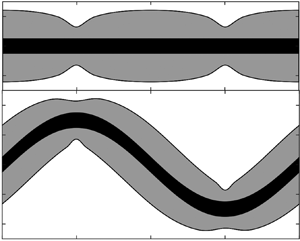
An impression of the yielded sheath around the swimmer is displayed in figure 6, which shows the yield surfaces predicted in certain cross-sections through the swimmer for a range of values for  $a$ and
  $B_s$, and a particular choice of the scaled wavelength
  $\lambda /\mathcal {R}$ (which does not affect the wave speed or power in the slender limit). Not surprisingly, the yielded region becomes more localised as
  $B_s$ is increased. On the other hand, as long as
  $B_s$ is not small, variations in the wave amplitude can result in yield surfaces that lie at similar distances from the swimmer even while the swimming speed increases by almost an order of magnitude (compare, for example, figures 6c and 6f). However, for smaller
  $B_s$ and larger
  $a$, self-intersections of the yield surfaces can arise (e.g. figure 6g); the implied overlap of the yielded regions occurs when the span of the flow domain is no longer much smaller than the wavelength of the swimming stroke, and implies a break down of the slender-body theory approximation.

Figure 6. Yield surfaces (grey) around sinusoidal swimmer (black) with  $n=1$, wavelength
  ${\lambda }/\mathcal {R} = 40$, Bingham number
  $B_s = 0.1$ (a,d,g),
  $B_s = 1$ (b,e,h) and
  $B_s = 100$ (c, f,i), and amplitude (scaled by the wavelength)
  $a=0.05$ (a–c),
  $a=0.1$ (d–f) and
  $a=0.15$ (g–i). The swimming speed is included in each panel (red). For the lowest
  $B_s$, only the plane of the wave is shown; higher
  $B_s$ solutions also include the out-of-plane yield surfaces (upper plots in each panel).
The characteristics displayed by the numerical results in these figures motivate a discussion of a number of limits of the problem, which we discuss below.
3.1. Newtonian limit
When  $n=1$ and
  $Bi\ll 1$, the force components have the limits in (2.7), and the constraint (2.19) reduces to
 \begin{equation} W_s = 1 - Q \left[ \int_{{-}1/2}^{1/2} (2 \tan^2\varPhi + 1) \cos\varPhi \, {\rm d} \zeta \right]^{{-}1} . \end{equation}
For a sinusoidal wave profile, we then recover a result derived by Hancock (Reference Hancock1953),
 \begin{equation} W_s = 1 - \int_{{-}1/2}^{1/2} \sqrt{1+4{\rm \pi}^2 a^2\cos^2 2{\rm \pi} \zeta}\,{\rm d}\zeta \left[ \int_{{-}1/2}^{1/2} \frac{1+8 {\rm \pi}^2 a^2 \cos^2 2{\rm \pi} \zeta} {\sqrt{1+4 {\rm \pi}^2 a^2\cos^2 2{\rm \pi} \zeta}}\, {\rm d} \zeta \right]^{{-}1} , \end{equation}
which gives  $W_s \sim 2 {\rm \pi}^2 a^2$ for small
  $a$. For a more general waveform, if
  $\chi \!=\! a \chi_1$ with
  $a\ll 1$, we set
  $\varPhi =a\varPhi _1\sim a \mathcal {X}_1'$ and
  $Q=1+a^2Q_2=1+\frac 12 a^2\int _0^1 \varPhi _1^2\, \textrm {d} \zeta$ (in view of (2.13) and (2.14)), and then find
  $W_s=a^2 W_2$ with
 \begin{equation} W_2 \sim \int_{{-}1/2}^{1/2} \varPhi_1^2\, {\rm d} \zeta .\end{equation}
3.2. Low-amplitude plastic swimming
For low-amplitude swimming with a yield stress, we again set  $\varPhi =a\varPhi _1\sim a \mathcal {X}_1', Q=1+a^2Q_2$ and
  $W_s=a^2 W_2$. Away from the extrema of the waveform, (2.17) and (2.18) then imply that
  $V+O(a)$ and
 \begin{equation} \delta \sim \frac12{\rm \pi}\,{\rm sgn}(\varPhi_1) - \frac{a}{\varPhi_1} \left(Q_2+\frac12\varPhi_1^2+W_2\right),\end{equation}
Over small regions surrounding those extrema, however, the wave slope  $\varPhi$ becomes smaller, leading to different scalings of the translation speed and motion direction. In particular, where
  $\varPhi =O(a^2)$, we find that
  $V = O(a^2)$ and
 \begin{equation} \delta \sim \tan^{{-}1} \frac{\varPhi_1}{a(Q_2+W_2)},\end{equation}
(assuming  $Q_2+W_2>0$), so that
  $\delta$ runs through the entire range
  $[-\frac 12{\rm \pi},\frac 12{\rm \pi} ]$.
Because  $V$ is therefore always small, the low-amplitude limit corresponds to
  $Bi=O(a^{-n})\gg 1$ or larger, as long as
  $B_s$ is non-zero (see (2.12)). This implies that the force components are given by the plastic limit
  $Bi\gg 1$. The angle of motion
  $\delta$, on the other hand, varies across its entire range (i.e.
  $\delta$ is not restricted to the narrow reorientation window; that limit, relevant for larger amplitude swimming, is considered below in § 3.3). As discussed further in Appendix A.3, the force components in this plastic limit take the form
 \begin{equation} F_x(\delta,n,Bi) \sim{-} Bi f_x(|\delta|) \, {\rm sgn} (\delta) \quad F_z(\delta,n,Bi) \sim{-} Bi f_z(|\delta|) \, {\rm sgn} (\cos\delta), \end{equation}
for some functions  $f_x$ and
  $f_z$. These functions can be determined from extrapolations of numerical results for
  ${Bi} \gg 1$, as plotted in figure 9 in the appendix. We note further the limiting value
  $f_x(\frac 12{\rm \pi} )\equiv 4 ({\rm \pi} +2\sqrt 2)$ and that
 \begin{equation} f_z(|\delta |) \approx A (\tfrac12 {\rm \pi}- |\delta|),\end{equation}
provides a good fit to the numerical data with  $A\approx 4.4$.
In view of (3.6), the constraint of vanishing drag (2.19) becomes
 \begin{equation} A \int_{{-}1/2}^{1/2} \left(\frac12{\rm \pi}-|\delta|\right)\,{\rm d} \zeta \sim a \int_{{-}1/2}^{1/2} f_x(|\delta|) |\mathcal{X}_1'| \,{\rm d}\zeta, \end{equation}
which is independent of  $n$. The forms for
  $\delta$ identified in (3.4) and (3.5) now imply that the contributions to the integrals in (3.8) arise from a ‘global’ region where
  $(\varPhi,\chi) = O(a)$ and
  $\delta$ is close to
  $\pm \frac 12{\rm \pi}$, and from narrow ‘local’ regions near the waveform's extrema, where
  $\varPhi = O(a^2)$ and
  $\delta$ varies. For symmetrical waveforms,
  $\mathcal {X}(\zeta )=-\mathcal {X}(-\zeta )$ and
  $\mathcal {X}(\zeta )=\mathcal {X}(\frac 14-\zeta )$, with extrema
  $\mathcal {X}(\pm \frac 14)=\pm 1$, the leading-order global contributions to the left- and right-hand sides of (3.8) are
 \begin{equation} 2a A + 4a A (Q_2+W_2) \int_0^{1/4-{\varepsilon}} \frac{{\rm d} \zeta}{|\mathcal{X}_1'|} \quad {\rm and\ } \quad 4a f_x\left(\frac12{\rm \pi}\right),\end{equation}
respectively, where we have introduced a splitting point  ${\varepsilon }$, satisfying
  $a\ll {\varepsilon }\ll 1$, to separate the global and local regions (Hinch Reference Hinch1991). The left-hand side of (3.8) has two local contributions from the
  $O({\varepsilon })$ regions around
  $|\zeta | = \frac 14$, each of which is equal to
 \begin{equation} \frac{2 a A (Q_2+W_2)}{|\mathcal{X}_1''(\frac14)|} \int_0^{\varDelta} \left(\frac12{\rm \pi}-\tan^{{-}1}{\tau} \right) \,{\rm d} {\tau}, \quad {\varDelta} = \frac{{\varepsilon} |\mathcal{X}_1''(\frac14)|}{a(Q_2+W_2)}.\end{equation}
The integrals in (3.9) and (3.10) diverge logarithmically for  ${\varepsilon }\to 0$. In writing the full constraint, we therefore reorganise accordingly to arrive at the implicit equation,
 \begin{equation} (Q_2+W_2) \left\{ J + \log\left[\frac{|\mathcal{X}_1''(\frac14)|}{a(Q_2+W_2)} \right]\right\} \sim \frac{f_x(\frac12{\rm \pi})-\frac12 A}{A} \left|\mathcal{X}_1''\left(\frac14\right)\right|,\end{equation}
with
 \begin{equation} J = \left[ \left|\mathcal{X}_1''\left(\frac14\right)\right| \int_0^{1/4-{\varepsilon}} \frac{{\rm d} \zeta}{|\mathcal{X}_1'|} - \log{\varepsilon}^{{-}1} \right]_{{\varepsilon}\to0} + 1 . \end{equation}
For the sinusoidal waveform,  $J\approx 1.24$, and the predictions from (3.11) are included in figure 3(d). The results are surprisingly close to the corresponding Newtonian prediction (§ 3.1), at least over the range of amplitudes and rheological parameters used in the plot.
Equation (3.11) implies the presence of a potentially non-asymptotic  $\log a^{-1}$ term, which demands that
  $W_s \to 1 - Q < 0$ for sufficiently small
  $a$. That is, the swimmer must inevitably reverse direction at very low amplitudes. For the sinusoidal waveform, the other factors in (3.11) conspire to arrange the speed reversal to arise for
  $a<10^{-7}$, far less that the range of amplitudes used in figure 3. Figure 7 shows results for different waveforms given either by the sawtooth-like profile,
 \begin{equation} \mathcal{X} = \sum_{j=1}^{16}\frac{({-}1)^{j-1}}{8{\rm \pi}^2(2j-1)^2} \sin [2{\rm \pi}(2j-1)\zeta] , \end{equation}
or the smoothed square wave,
 \begin{equation} \mathcal{X} = \frac{\tanh ( \varsigma \sin 2{\rm \pi}\zeta )}{\tanh\varsigma},\end{equation}
where  $\varsigma$ is a smoothing parameter. For the latter, the speed reversal is observed for higher amplitudes provided the wave is sufficiently sharp (i.e.
  $\varsigma$ large enough). The fact that such strokes lead to the body swimming backwards implies a far more significant rheological effect than has been noted for other complex fluids. It also implies the curious result that if the ambient fluid has a yield stress, there is a non-zero amplitude with which the swimmer can undulate whilst remaining stationary.

Figure 7. Swimming speed  $W_s$ against amplitude
  $a$ for
  $n=1$ and waveforms given by the sawtooth profile (3.13) (green) or smoothed square wave (3.14) with
  $\varsigma =0.01$, 1,
  $1.5$, 2,
  $2.75$, 4 and 6 (from blue to red). In (a), the low-amplitude range is shown, with the solid lines showing the solution of (3.11) and the stars indicating numerical solutions, all with
  $B_s=10^3$. In (b), higher amplitudes are shown, together with more numerical solutions with
  $B_s=5$ (dashed) and 50 (solid). The inset in (a) displays the waveforms.
The dissipation rate associated with this low-amplitude plastic swimming can be computed from (2.20), and reduces to the left-hand side of (3.8), up to a factor of  $B_s$, in this limit. Thus the dissipation is
  $\mathcal {P} \sim 4 a f_x(\frac 12 {\rm \pi}) B_s \sim 16 ({\rm \pi} + 2\sqrt {2}) a B_s$, which, unlike the swimming speed, is independent of the swimming gait (see figure 4) and scales linearly with the swimming amplitude
  $a$. The efficiency (2.21) is
  $\eta \sim 2{\rm \pi} B_s |W_s| / \mathcal {P}$ in this limit, and thus depends sensitively on the swimming gait through the dependence on
  $W_s$. For the sinusoidal swimmer, figure 5 shows that the efficiency in a Newtonian fluid is far lower than in a viscoplastic fluid for small
  $a$; this trend must become interrupted as
  $a$ is decreased further, however, because
  $W_s$ vanishes at some non-zero amplitude in the viscoplastic case.
3.3. Plastic sliding or burrowing
The numerical results in figure 3 indicate that  $W_s$ approaches the wave speed for sufficiently strong amplitudes and yield stresses. Our rationalisation of this observation is that at such parameter settings, the swimmer is able to exploit the strong drag anisotropy for small
  $\delta$ that is created by the narrow reorientation window (discussed § 2.1), in order to ‘slide’ through the medium without appreciable drift. That is, each segment of the swimmer travels in essentially its local axial direction, while the associated force on that segment can be directed at a wide range of angles
  $\delta _f$. Suppose the swimmer is in this limit, with swimming speed
  $W_s = 1-\epsilon$ and
  $\epsilon \ll 1$. Then,
 \begin{equation} V \sim Q - {\epsilon} \cos \varPhi \quad \& \quad \delta \sim \tan^{{-}1} \frac{{\epsilon}\sin\varPhi}{Q} = \frac{{\epsilon}}{Q} \sin\varPhi + \cdots. \end{equation}
Consequently, given the limits of the force components in (2.9a,b),
 \begin{equation} V^n(F_x \sin\varPhi - F_z \cos{\varPhi}) \sim {\rm \pi}B_s \left[ 2 \cos\varPhi - \frac{{\epsilon} \alpha_n B_s^{2/(n+1)}}{Q^{(3n+1)/(n+1)}} \sin^2\varPhi \right], \end{equation}
and the force-balance condition (2.19) demands that
 \begin{equation} {\epsilon} \sim \mathcal{E}(a,n,B_s) \equiv \frac{2 Q^{(3n+1)/(n+1)} B_s^{{-}2/(n+1)} }{\alpha_n I}, \quad I(\textit{a}) = \int_{{-}1/2}^{1/2} \sin\varPhi\tan\varPhi \,{\rm d} \zeta. \end{equation}
The convergence of  $1-W_s$ to
  $\mathcal {E}(a,n,B_s)$ is confirmed by the numerical solutions, as displayed in the inset of figure 3(c).
We expect this theory to hold as long as  $\delta$ lies within the narrow reorientation window, which requires
  $\alpha _n Bi^{2/(n+1)} \delta \lesssim \beta$, for some number
  $\beta$ that we compute to be approximately 5 (see Appendix A.2 and figure 8). That is,
 \begin{equation} |\delta| \lesssim \frac{\beta}{\alpha_n} Bi^{{-}2/(n+1)} \implies|\sin\varPhi | \lesssim \frac12 \beta I(\textit{a}) \approx \frac{5}{2}I(\textit{a}),\end{equation}
independent of  $n$, at every point along the swimmer's body. Given the specific sinusoidal waveform in (2.4), this requirement reduces to
  $a \gtrsim 0.12$. Simultaneously, however, the swimming stroke should also fall within the plastic limit
  $Bi\gg 1$, which restricts the range of possible values of
  $B_s$; see the inset in figure 3(c), which demonstrates that
  $\mathcal {E}(a,n,B_s)$ must be small.

Figure 8. The force direction  $\delta _f$ against
  $\alpha _n{Bi}^{{2}/({n+1})} \delta$ for
  $n=\frac 12$ (blue),
  $n=1$ (black) and
  $n=2$ (red), with
  $Bi=2^{j+n}$ and
  $j=3, 4, \ldots, 10$. The thick (green) dashed lines shows the prediction
  $\delta _f \sim \tan ^{-1}(\frac 12\alpha _n{Bi}^{{2}/({n+1})} \delta )$. The vertical dotted line at
  $\alpha _n{Bi}^{{2}/({n+1})} \delta =5$ roughly locates the window of strong force anisotropy.
As discussed in Appendix A.2, the flow around the cylindrical body in the narrow reorientation window becomes restricted to a viscoplastic boundary layer. Consequently, in this form of burrowing locomotion the deformations are strongly localised, and the swimmer slides along a conduit that is only slightly bigger than its body. This feature is illustrated by the yield surfaces in the final column of figure 6.
Note that the condition in (3.18) is relatively insensitive to the waveform, being  $a\lesssim 0.11 - 0.12$ for a variety of different profiles, including the sinusoid, sawtooth (3.13) and smoothed square waves (3.14). This feature can be seen in figure 7(b), where the speed data for
  $B_s=50$ and
  $10^3$ approach the limit
  $W_s\approx 1$ for such amplitudes, independently of the waveform.
The dissipation rate or power output in this limit reduces to  $\mathcal {P} \sim 2{\rm \pi} Q^2 B_s$, as shown in figure 4. The factor of
  $V^n F_z(0,n,Bi) \equiv 2{\rm \pi} B_s$ arises from the need to exceed the yield stress around the unit radius of the swimmer in this limit, while the dependence on
  $Q^2$, and thus on the swimming gait and amplitude, follows because the swimmer's body must travel along a distance of the arclength
  $Q$ at a speed of
  $Q$ each wavelength. The power required to drag the straightened swimmer axially at the (unit) swimming speed is lower by a factor of
  $Q$, leading to an efficiency of
  $\eta \sim 1/Q$; cf. figure 5. The efficiency is thus maximised at the smallest amplitude for which the burrowing state can be attained, which is
  $a\approx 0.11 - 0.12$. Dependence on the waveform enters through
  $Q$: the maximal efficiency is given by the sawtooth triangle wave (3.13), as in the Newtonian problem (see Lighthill Reference Lighthill1975), although the maximum is here given by
  $\eta \approx 90\,\%$ at
  $a=0.12$. For comparison, the peak efficiencies are
  $\eta (0.12) \approx 88\,\%$ for the sinusoidal waveform and
  $\eta (0.12) \approx 68\,\%$ for the square wave in (3.14); in all cases, these numbers are an order of magnitude higher than their Newtonian equivalents.
4. Conclusion
In this paper, we have generalised a previous viscoplastic slender-body theory (Hewitt & Balmforth Reference Hewitt and Balmforth2018) and applied it to the problem of locomotion through a viscoplastic ambient fluid driven by a waving cylindrical filament. For low-amplitude waves, the stresses become dominated by the yield stress and the problem reduces to that for swimming through a perfectly plastic medium (more specifically, a rigid-plastic material with the von Mises yield condition, given our use of the Herschel–Bulkley viscoplastic constitutive law). A curious feature of this limit is that the swimming speed must become negative (i.e. the swimmer moves in the same direction as the wave) if the wave amplitude is sufficiently small relative to its wavelength. This phenomenon requires very small amplitudes and results in extremely small speeds when the swimmer employs a sinusoidal waveform, but is more pronounced with a square-wave-like swimming gait.
When wave amplitudes are not so small and for larger yield stresses, a key feature of viscoplastic slender-body flow comes into play: unless the motion is very closely directed along the axis of each cylindrical filament of the body, significant sideways forces arise. Only in almost axial motion does the drag force become closely aligned with the direction of motion. In the locomotion problem, the appreciable anisotropy in the drag that is set up across the narrow angular ‘reorientation’ window allows the swimmer to burrow through the medium by sliding along its axis at nearly the wave speed.
An analysis of this limit of plastic sliding or burrowing indicates that the wave amplitude need not be particularly large to achieve this burrowing motion (the wave amplitude needs to be approximately one eighth of the wavelength), a result that is insensitive to the specific waveform of the swimmer. There is no obvious advantage in employing a higher wave amplitude than this, because the swimming speed cannot increase past the wave speed whereas the power expended by the swimmer continues to increase with wave amplitude. Indeed, this result is clearly demonstrated by considering the swimming efficiency  $\eta$, which compares the power consumption by swimming with that required to drag the straightened body at the same locomotion speed. The efficiency can become relatively large in the burrowing limit (an order of magnitude higher than the Newtonian equivalent) because dragging and burrowing differ only in the higher body speed of the undulating swimmer. Importantly, because this style of locomotion is characteristic of nearly plastic deformation in the surrounding medium, the ability to burrow in this manner is not limited to a viscoplastic fluid, but should characterise any plastic material such as a cohesive granular medium like wet sand.
Burrowing of this kind has been observed experimentally for various worms that naturally inhabit wet sediments or soils. Dorgan et al. (Reference Dorgan, Law and Rouse2013), for example, measured the motion of the polychaete worm Armandia brevis through sediments and found that the worms burrowed along their axis at a swimming speed essentially equal to the wave speed (that is, a dimensionless wave speed or ‘wave efficiency’ of  $1$). They observed that the worms burrowed with a scaled amplitude (relative to wavelength) of
  $a \approx 0.18$, which is consistent with our theoretical prediction for being in the burrowing limit (
 $a\gtrsim 0.12$). Although we cannot be certain whether these swimmers operate in the plastic limit, having no access to the detailed rheology of the ambient, support for this conclusion is also provided by the fact that these observations were insensitive to the swimmer's wave frequency (and thus wave speed), consistent with our theory when
  $B_s$ is sufficiently large. Further, the same worms swimming in water displayed an inability to burrow along their axis, presumably because of the absence of a plastic yield stress, and instead ‘drifted’ with a much slower, frequency-dependent, translation speed.
Similarly, observations of burrowing sand lances (Gidmark et al. Reference Gidmark, Strother, Horton, Summers and Brainerd2011) and ocellated skinks (Sharpe, Kuckuk & Goldman Reference Sharpe, Kuckuk and Goldman2015) have also revealed locomotion speeds reaching those of propulsive undulations with  $a\approx 0.25 - 0.35$. While the relevance of plasticity in the ambient material to enable this form of burrowing locomotion has already been recognised (Dorgan Reference Dorgan2015), the present study provides the first theoretical framework in which to describe such slender motion through a viscoplastic ambient. Further comparison of theory and observation is certainly warranted, but requires a detailed characterisation of ambient rheology. A consideration of the dynamics at the head of the swimmer, where the conduit followed by burrowing is opened, may also be worthwhile. Finally, the framework presented here could be extended in the future to describe other forms of observed locomotion such as peristalsis (Kudrolli & Ramirez Reference Kudrolli and Ramirez2019).
Supplementary material
Supplementary material are available at https://doi.org/10.1017/jfm.2022.48.
Declaration of interests
the authors report no conflict of interest.
Appendix A. Analysis
A.1. Formulation
In this appendix we quote the dimensionless governing equations used to generate the slender-body results discussed in § 2.1: that is, for viscoplastic flow around an infinitely long, straight cylinder translating at an angle  $\delta$ to its axis (see also Hewitt & Balmforth Reference Hewitt and Balmforth2018). Lengths are scaled by the cylinder radius
  $\mathcal {R}$, velocities by the translation speed
  $\mathcal {U}$ of the cylinder and stresses by
  $K(\mathcal {U}/\mathcal {R})^n$. In the cylindrical polar coordinates system
  $(r,\theta,z)$ aligned with the centreline, (2.3) becomes
 $$\begin{gather} \frac{1}{r}\frac{\partial}{\partial r}(ru) + \frac{1}{r} \frac{\partial v}{\partial \theta} = 0, \end{gather}$$
 $$\begin{gather}\frac{\partial p}{\partial r} = \frac{1}{r}\frac{\partial}{\partial r}(r\tau_{ rr})+ \frac{1}{r}\frac{\partial}{\partial \theta}\tau_{ r\theta} - \frac{\tau_{\theta\theta}}{r}, \quad \frac{1}{r}\frac{\partial p}{\partial \theta} = \frac{1}{r^2}\frac{\partial}{\partial r}(r^2\tau_{r\theta})+ \frac{1}{r}\frac{\partial}{\partial \theta}\tau_{\theta\theta}, \end{gather}$$
 $$\begin{gather} 0 = \frac{1}{r}\frac{\partial}{\partial r}(r\tau_{ rz})+ \frac{1}{r}\frac{\partial}{\partial \theta}\tau_{\theta z}, \end{gather}$$
where subscripts indicate tensor components. The dimensionless version of the Herschel–Bulkley law (2.1) is
 \begin{equation} \tau_{ ij} = \left( {\dot\gamma}^{n-1} + \frac{{Bi}}{{\dot\gamma}}\right) {\dot\gamma}_{ ij} \quad {\rm for} \ \tau>{Bi}, \end{equation}
and  ${\dot \gamma }_{ ij}=0$ otherwise, where
 \begin{equation} \{ {\dot\gamma}_{ ij} \} = \left( \begin{matrix} 2u_r & v_r+(u_\theta-v)/r & w_r \\ v_r+(u_\theta-v)/r & 2(v_\theta+u)/r & w_\theta/r \\ w_r & w_\theta/r & 0 \end{matrix} \right) , \end{equation}
and subscripts of  $r$ and
  $\theta$ on the velocity components denote partial derivatives. The translation of the cylinder demands the boundary conditions
  $(u,v,w)=(\cos \theta \sin \delta,-\sin \theta \sin \delta,\cos \delta )$ at
  $r=1$. In the far field, the stresses must eventually fall below the yield stress and the fluid must plug up, such that
  $(u,v,w)\to (0,0,0)$. The net drag per unit length exerted on the cylinder is
  $\hat {\boldsymbol x} F_{ x} + \hat {\boldsymbol z} F_{ z}$, with
 \begin{gather} \left[\begin{matrix} F_x \\F_z \end{matrix}\right] = \oint \left[\begin{matrix} ({-}p+\tau_{rr})\cos\theta-\tau_{r\theta}\sin\theta \\ \tau_{rz} \end{matrix}\right]_{r=1}\, {\rm d} \theta = \oint \left[\begin{matrix} 2 \tau_{rr} \cos\theta + (r \tau_{r\theta})_r \sin\theta \\\tau_{rz} \end{matrix}\right]_{r=1}\, {\rm d} \theta . \end{gather}
We solve these equations numerically using an augmented Lagrangian finite-difference scheme, employing a Fourier transform in the azimuthal direction. The scheme differs from that used in Hewitt & Balmforth (Reference Hewitt and Balmforth2018) only by the inclusion of a nonlinear viscosity to capture shear thinning or thickening for  $n\neq 1$.
A.2. Axial and nearly axial motion: force reorientation
For purely axial motion, we have
 \begin{equation} r \tau_{rz} ={-}r_p {Bi} \quad \& \quad \tau_{rz} ={-}{Bi} - ({-}w_r)^n, \end{equation}
where  $r=r_p$ denotes the (axisymmetrical) yield surface for which
  $\tau _{rz}=-{Bi}$ (
 $w_r<0$), given that
  $w=1$ on
  $r=1$ and decreases to
  $w=0$ with
  $w_r=0$ at
  $r=r_p$. Hence,
 \begin{equation} w = 1-\int_1^r \left[ (r_p-r) \frac{{Bi}}{r}\right]^{1/n}\, {\rm d} r . \end{equation}
In the limit of a thin gap, for  ${Bi}\gg 1$, we have
  $r=1+{Bi}^{-1/(1+n)}\xi$ and
 \begin{equation} w_\xi \sim{-} (\xi_p-\xi)^{1/n}, \quad w \sim \frac{n}{n+1}(\xi_p-\xi)^{(n+1)/n} \quad \& \quad \xi_p = \left( 1+\frac{1}{n}\right)^{{n}/({n+1})}, \end{equation}
where  $\xi =\xi _p$ denotes the rescaled yield surface. Because the axial shear stress
  $\tau _{rz}\sim -{Bi}$ in this limit, the axial force is given by
  $F_z \sim - 2{\rm \pi} {Bi}$, corresponding to the perfectly plastic limit for a cylinder translating along its axis.
If, instead, the motion is nearly, but not exactly, aligned with the axis, and  ${Bi}\gg 1$, the sideways translation is largely contained within
  $1< r< r_p$ or
  $0<\xi <\xi _p$, and the leading-order shear rate is
  ${\dot \gamma }\sim (\xi _p-\xi )^{1/n}$. The lateral force balances demand that
 \begin{equation} \frac{\partial p}{\partial \xi}\sim 0, \quad \frac{\partial p}{\partial \theta} \sim {Bi}^{{1}/({n+1})} \frac{\partial \tau_{r\theta}}{\partial \xi} \sim {Bi}^{({n+2})/({n+1})} \frac{\partial }{\partial \xi} \left[ \frac{v_\xi}{(\xi_p-\xi)^{1/n}} \right], \end{equation}
since
 \begin{equation} \tau_{r\theta} \sim \frac{{Bi} \, v_r}{|w_r|} \sim \frac{{Bi} \, v_\xi}{(\xi_p-\xi)^{1/n}} . \end{equation}
But  $v=O(\delta )$ at
  $\xi =0$ and
  $v(\xi _p,\theta )=0$, and so
 \begin{equation} v \sim{-} \frac{n\xi (\xi_p-\xi)^{1+1/n} }{2n+1} {Bi}^{-({n+2})/({n+1})}\frac{\partial p}{\partial \theta} , \end{equation}
as long as  $\delta \ll O({Bi}^{-({n+2})/({n+1})}p)$, which turns out to be the case.
The continuity relation implies a radial velocity  $u$ given by
 \begin{equation} u_\xi \sim {Bi}^{-{1}/({n+1})} v_\theta \sim \frac{n\xi (\xi_p-\xi)^{1+1/n} }{2n+1} {Bi}^{-({n+3})/({n+1})}\frac{\partial^2 p}{\partial \theta^2} , \end{equation}
or
 \begin{equation} u \sim{-} \frac{n^2 (\xi_p-\xi)^{2+1/n}[n\xi_p + (2n+1)\xi] }{(2n+1)^2(3n+1)} {Bi}^{-({n+3})/({n+1})}\frac{\partial^2 p}{\partial \theta^2} , \end{equation}
if  $u=0$ at
  $\xi =\xi _p$. But we also have that
  $u = \delta \cos \theta$ at
  $\xi =0$, and so
 \begin{equation} p \sim \frac{(2n+1)^2(3n+1)}{n^3 \xi_p^{3+1/n} } {Bi}^{({n+3})/({n+1})} \delta \cos\theta. \end{equation}
Finally,
 \begin{equation} F_x \sim{-} \oint p\cos\theta \, {\rm d}\theta \sim{-} \alpha_n {\rm \pi}{Bi}^{({n+3})/({n+1})} \delta , \end{equation}
where  $\alpha _n$ is defined in (2.10). The transverse force therefore becomes dominated by the axial force
  $F_z=O(Bi)$ only when
  $\delta \ll O(Bi^{-2/(n+1)})$. The collapse of the force direction
  $\delta_f$ when plotted against
  $\alpha _n{Bi}^{{2}/({n+1})} \delta$ for different
  $n$ (and large
  $Bi$) is illustrated in figure 8; also included is the prediction
  $\delta _f \sim \tan ^{-1}(\frac 12\alpha _n{Bi}^{{2}/({n+1})} \delta )$ based on the preceding results.
A.3. Plastic solutions outside the narrow window of force reorientation
The nearly plastic solutions outside the narrow window where the force becomes reorientated are illustrated in figure 9. These solutions are characterised by a region of almost plastic deformation surrounding the cylinder over distances of order the radius. The perfectly plastic flow is buffered by viscoplastic shear layers where the viscous stress remains important, and the two shear stress components  $\tau _{nz}$ and
  $\tau _{sn}$ dominate the stress tensor. Here,
  $s$ denotes the arclength along the centreline of the boundary layer and
  $n$ is the transverse coordinate in the plane of the cylinder's cross-section. Of key importance is the shear layer against the cylinder, which transmits the fluid drag.

Figure 9. Numerical solutions showing the deformation rate invariant  ${\dot \gamma }$ (as a density over the
  $(x,y)$-plane) and flow pattern (which has vertical symmetry; here showing streamlines of the planar velocity field
  $u\hat {\boldsymbol {x}}+v\hat {\boldsymbol {y}}$ in the upper half-plane (blue); and contours of constant axial speed
  $w$ in the lower half-plane (green)) around a moving cylinder for
  $Bi=1024$ and
  $n=1$. The angle of inclination, shown pictorially in blue at the centre of each cylinder, is (a)–(d)
  $2{\rm \pi} ^{-1}\delta = [\frac 34,\frac 12, 0.1,0.05]$. Panels (e) and ( f) show the scaled drag components
  $(|F_x|,|F_z|)/Bi$ and direction
  $\delta _f$ against
  $\sqrt {2{\rm \pi} ^{-1}\delta }$ for
  $n=\frac 12$ (dashed),
  $n=1$ (solid) and
  $n=2$ (dotted), with
  $Bi=2^{j+n}$ and
  $j=3, 4, \ldots, 10$. The thick (red) dashed lines show the approximations
  $f_x(|\delta |)$ (extrapolated from the numerical results) and
  $f_z(|\delta |) = A(\frac 12 {\rm \pi}- |\delta |)$ with
  $A=4.4$, as quoted in § 3.2, and the stars indicate the analytical results for pure axial or transverse motion. The (red) points in ( f) indicate the motion angles used for (a)–(d).
In the plastic limit,  $Bi\to \infty$, the boundary layers become infinitely thin and feature jumps in tangential velocity. The corresponding plastic solution satisfies the slip conditions,
 \begin{equation} \begin{pmatrix} \tau_{nz} \\\tau_{sn}\end{pmatrix} ={-} \frac{Bi}{\sqrt{V^2+W^2}} \begin{pmatrix} W \\V \end{pmatrix},\end{equation}
where  $V$ and
  $W$ denote the jumps in the tangential velocity components, which can be extracted from a boundary-layer analysis like that used above. It does not seem possible to analytically find the limiting plastic solution for general
  $\delta$ (the method of sliplines, which proves useful in the purely two-dimensional flow problem, is not available here). For
  $\delta \to \frac 12{\rm \pi}$, the transverse motion of the cylinder dominates the axial translation, which enters as a regular perturbation of the two-dimensional problem solved by Randolph & Houlsby (Reference Randolph and Houlsby1984). In particular, one may calculate the transverse drag
  $f_x(\frac 12{\rm \pi} )$ as quoted in § 3.2. We also observe that the linear approximation (3.7) for
  $f_z$ works well nearly all the way up to the reorientation window.
The limit  ${Bi}\gg 1$ and
  $Bi^{-2/(n+1)}\ll \delta \ll 1$ is somewhat curious, as it corresponds to the sliding of a cylinder in the direction of its length through a perfectly plastic medium with an arbitrarily small (as long as
  $Bi$ can be taken sufficiently large) but non-zero sideways translation. Associated with this motion is a finite transverse drag (the force angle approaches a value close to
  $\frac 13{\rm \pi}$) and a flow pattern like that in figure 9(d) (save for the viscoplastic boundary layers, which shrink to slip surfaces as
  ${Bi} \to \infty$). Of course, the transverse drag eventually declines, and the flow pattern is consumed by the boundary layer of the axial velocity, as the motion aligns with the axis within the reorientation window. However, this requires a viscous effect (i.e. finite
  $Bi$). The origin of this curious feature is in the perfectly plastic solution itself: for pure axial motion, there is no deformation of the fluid, with the translation of the cylinder permitted by slip along its surface. But sideways translation cannot be accommodated by this style of motion, no matter how small, which instead demands plastic deformation over a finite region.


 Open access