Hostname: page-component-7bb8b95d7b-qxsvm Total loading time: 0 Render date: 2024-09-28T16:59:56.747Z Has data issue: false hasContentIssue false

Learn to flap: foil non-parametric path planning via deep reinforcement learning

Published online by Cambridge University Press:  27 March 2024
Z.P. Wang
Affiliation:
School of Engineering, Westlake University, Hangzhou, Zhejiang 310024, PR China School of Mechanical and Material Engineering, Queen's University, Kingston, ON K7L 3N6, Canada
R.J. Lin
Affiliation:
University of Chinese Academy of Sciences, Beijing 100049, PR China Institute of Automation, Chinese Academy of Sciences, Beijing 100190, PR China
Z.Y. Zhao
Affiliation:
University of Chinese Academy of Sciences, Beijing 100049, PR China Institute of Automation, Chinese Academy of Sciences, Beijing 100190, PR China
X. Chen
Affiliation:
Taihu Laboratory of Deepsea Technological Science, Wuxi, Jiangsu 214000, PR China
P.M. Guo*
Affiliation:
School of Engineering, Westlake University, Hangzhou, Zhejiang 310024, PR China School of Mechanical and Material Engineering, Queen's University, Kingston, ON K7L 3N6, Canada
N. Yang*
Affiliation:
University of Chinese Academy of Sciences, Beijing 100049, PR China Institute of Automation, Chinese Academy of Sciences, Beijing 100190, PR China
Z.C. Wang
Affiliation:
Laboratory of Ocean Energy Utilization of Ministry of Education, Dalian University of Technology, Dalian 116024, PR China School of Energy and Power Engineering, Dalian University of Technology, Dalian 116024, PR China
D.X. Fan*
Affiliation:
School of Engineering, Westlake University, Hangzhou, Zhejiang 310024, PR China
*
Email addresses for correspondence: [email protected], [email protected], [email protected]

Abstract

To optimize flapping foil performance, in the current study we apply deep reinforcement learning (DRL) to plan foil non-parametric motion, as the traditional control techniques and simplified motions cannot fully model nonlinear, unsteady and high-dimensional foil–vortex interactions. Therefore, a DRL training framework is proposed based on the proximal policy optimization algorithm and the transformer architecture, where the policy is initialized from the sinusoidal expert display. We first demonstrate the effectiveness of the proposed DRL-training framework, learning the coherent foil flapping motion to generate thrust. Furthermore, by adjusting reward functions and action thresholds, DRL-optimized foil trajectories can gain significant enhancement in both thrust and efficiency compared with the sinusoidal motion. Last, through visualization of wake morphology and instantaneous pressure distributions, it is found that DRL-optimized foil can adaptively adjust the phases between motion and shedding vortices to improve hydrodynamic performance. Our results give a hint of how to solve complex fluid manipulation problems using the DRL method.

Type
JFM Papers
Copyright
© The Author(s), 2024. Published by Cambridge University Press

1. Introduction

The design of novel bioinspired flapping propulsors has garnered considerable interest within the scientific community (Licht et al. Reference Licht, Polidoro, Flores, Hover and Triantafyllou2004). As Lighthill eloquently stated, ‘about $10^9$ years of animal evolution … have inevitably produced rather refined means of generating fast movement at low energy cost’ (Lighthill Reference Lighthill1969). Indeed, when compared with traditional man-made aquatic transportation methods (Low Reference Low2011), nature offers alternative solutions that have proven to be more agile and effective in overcoming the constraints posed by aquatic environments (Fish Reference Fish1993; Jayne & Lauder Reference Jayne and Lauder1995; Domenici & Blake Reference Domenici and Blake1997; Triantafyllou, Weymouth & Miao Reference Triantafyllou, Weymouth and Miao2016). For instance, consider the vortical wake generated behind a rigid hull submarine, which results in energy losses due to flow separation, ultimately leading to a significant loss of propulsive efficiency (Newman Reference Newman1977). On the contrary, aquatic animals employ oscillatory actuation techniques (Triantafyllou, Triantafyllou & Yue Reference Triantafyllou, Triantafyllou and Yue2000) that can reduce flow separation, recover losses incurred by their bodies (Barrett et al. Reference Barrett, Triantafyllou, Yue, Grosenbaugh and Wolfgang1999) and even harness energy from unsteady oncoming flows (Beal et al. Reference Beal, Hover, Triantafyllou, Liao and Lauder2006).

To model animal oscillatory propulsion, many researchers have adopted a simplified model involving sinusoidally flapping foils with easily parameterized trajectories (Wu et al. Reference Wu, Zhang, Tian, Li and Lu2020). Notably, studies have highlighted the strong correlation between flapping efficiency and the Strouhal number ($Sr$), which is evident in its narrow optimal range across aquatic animals of varying sizes (Qi et al. Reference Qi2022). In addition, numerous research efforts have been dedicated to discovering a universal scaling law governing the wake patterns produced by flapping foils. For instance, Lagopoulos, Weymouth & Ganapathisubramani (Reference Lagopoulos, Weymouth and Ganapathisubramani2019) deduced that the foil's kinematics can serve as a parameterization for the drag-to-thrust wake transition. Moreover, investigations of the hydrodynamic characteristics of foils, such as thrust, side force, power coefficient and efficiency, based on sinusoidal motion, have yielded valuable insight over decades (Godoy-Diana, Aider & Wesfreid Reference Godoy-Diana, Aider and Wesfreid2008; Schnipper, Andersen & Bohr Reference Schnipper, Andersen and Bohr2009; Xiao & Zhu Reference Xiao and Zhu2014; Young, Lai & Platzer Reference Young, Lai and Platzer2014; Wu et al. Reference Wu, Zhang, Tian, Li and Lu2020). For example, Floryan et al. (Reference Floryan, Van Buren, Rowley and Smits2017) demonstrated that foil performance depends both on the Strouhal number and the reduced frequency.

However, recent observations have revealed that animals often employ non-sinusoidal motions, especially in complex group formations. For instance, Li et al. (Reference Li, Ashraf, François, Kolomenskiy, Lechenault, Godoy-Diana and Thiria2021) shed light on how fish can modulate a distinctive intrinsic cycle to maintain their desired speed in the burst-and-coast swimming gait. This unique swimming pattern not only allows fish to achieve their desired speed but also endows them with rapid manoeuvrability through substantial body flexing (Triantafyllou et al. Reference Triantafyllou, Weymouth and Miao2016). Furthermore, Chin & Lentink (Reference Chin and Lentink2016) conducted a study on the wing–wake interaction during stroke reversal in insects, which elucidates how they can travel efficiently. When fish travel in tandem or schooling formations with non-sinusoidal gaits, the resulting wake interactions and patterns become notably more complex, adding to the intrigue of their locomotion. Lagopoulos, Weymouth & Ganapathisubramani (Reference Lagopoulos, Weymouth and Ganapathisubramani2020) conducted a comprehensive examination of the influence of the downstream field on the front foil, providing further information on these complex interactions.

As flapping motions become more complex, their trajectories become less amenable to simple parameterization. Preliminary studies (Teng et al. Reference Teng, Deng, Pan and Shao2016; Liu, Huang & Lu Reference Liu, Huang and Lu2020; Ashraf, Wassenbergh & Verma Reference Ashraf, Wassenbergh and Verma2021) have examined various non-sinusoidal flapping trajectories and have demonstrated significant hydrodynamic enhancements that cannot be ignored. Biological investigations by Lighthill (Reference Lighthill1971) and Videler (Reference Videler1981) have revealed that such swimming gaits can substantially improve energy efficiency. However, this improvement is intricately linked to intrinsic and motion parameters specific to fish, rendering their intermittent dynamics incompatible with scaling laws designed for continuous swimming (Gazzola, Argentina & Mahadevan Reference Gazzola, Argentina and Mahadevan2014; Van Buren et al. Reference Van Buren, Floryan, Wei and Smits2018). In reality, even moderate changes in the instantaneous angle of attack can lead to significant alterations in forces, mainly attributed to intricate interactions between the foil and vortices (Izraelevitz & Triantafyllou Reference Izraelevitz and Triantafyllou2014). Therefore, the underlying flow mechanism of non-parametric foil flapping remains only partially explored and lacks clarity. This represents a quintessential nonlinear, unsteady and high-dimensional flow control problem (Gerhard et al. Reference Gerhard, Pastoor, King, Noack, Dillmann, Morzynski and Tadmor2003; Flinois & Morgans Reference Flinois and Morgans2016; Guéniat, Mathelin & Hussaini Reference Guéniat, Mathelin and Hussaini2016). Optimizing such non-parametric flapping trajectories presents a formidable challenge for traditional control techniques, often resulting in inefficient and intractable solutions.

Deep reinforcement learning (DRL) has recently gained significant attention in fluid mechanics for its astonishing achievement in solving complex problems, such as Atari (Silver et al. Reference Silver2017) and the three-dimensional maze game (Beattie et al. Reference Beattie2016), continuous control of underwater robot fish (Zheng et al. Reference Zheng, Zhang, Wang, Xiong and Xie2021; Zhang et al. Reference Zhang, Tian, Yang, Wang, Sun, Zhang and Xie2022), optimal control of nonlinear systems (Luo, Liu & Wu Reference Luo, Liu and Wu2017), pedestrian regulation (Wan et al. Reference Wan, Jiang, Fahad, Ni, Guo and He2018), traffic grid signal control (Tan et al. Reference Tan, Bao, Deng, Jin, Dai and Wang2019), robotics (Won, Müller & Lee Reference Won, Müller and Lee2020) and other industrial tasks (Degrave et al. Reference Degrave2022).

Recently, DRL has found applications in various flow control problems, achieving several notable successes. These successes encompass drag reduction for bluff bodies (Rabault et al. Reference Rabault, Kuchta, Jensen, Réglade and Cerardi2019; Fan et al. Reference Fan, Yang, Wang, Triantafyllou and Karniadakis2020) and lift enhancement for airfoils (Wang et al. Reference Wang, Mei, Aubry, Chen, Wu and Wu2022), where DRL has been employed to learn statistical mean control actions that induce favourable wake patterns. Furthermore, Verma, Novati & Koumoutsakos (Reference Verma, Novati and Koumoutsakos2018) implemented DRL to reveal how fish schooling could harvest energy in parametric motion. However, it is worth noting that optimizing foil flapping motions presents a distinct challenge. This challenge involves learning a coherent cyclical motion, meticulously manipulating the strength and timing of shedding vortices and effectively managing their interactions with the moving foil (Muhammad, Alam & Noack Reference Muhammad, Alam and Noack2022). These requirements extend beyond the capabilities of conventional DRL algorithms, which may not readily adapt to such complex tasks.

The present study introduces a DRL training framework based on the proximal policy optimization (PPO) algorithm and the transformer architecture. Notably, the policy is initialized using expert demonstrations rather than randomization. In our initial phase, we conduct a comprehensive comparison with other DRL training frameworks to ascertain the learning capabilities of the proposed agent in the context of flapping. Furthermore, by meticulously adjusting reward functions and action thresholds, we demonstrate substantial improvements in different optimization emphases related to thrust and efficiency through the learned non-parametric flapping trajectories. Finally, through flow visualization and the comparison of key hydrodynamic parameters, we provide insights into why the agent's flapping behaviour may outperform statistically equivalent sinusoidal motion.

This rest of the paper is organized as follows. In § 2, the physical and simulation models are presented with an emphasis on the DRL learning framework. Results are presented in § 3 on DRL learning results and their comparison with sinusoidal motions. To close, § 4 provides a summary and conclusions. In the appendices, we provide validation and verification of the simulation method as well as additional DRL learning results using a different reward function.

2. Materials and methods

2.1. Physical model

We numerically study a two-dimensional NACA0016 foil flapping in the uniform inflow at $Re = {U_\infty c}/{\nu } = 1173$, where $U_\infty$ is the uniform inflow velocity, $c$ is the foil chord length and $\nu$ is the fluid kinematic viscosity. The trajectory of the flapping foil is first prescribed as a sinusoidal motion combined with both heave $h_s(t)$ and pitch $\theta _s(t)$ around $c/4$. Therefore, the prescribed sinusoidal motion can be parameterized as follows:

(2.1)\begin{equation} \left.\begin{array}{c@{}} h_s(t) =h_0\sin(2{\rm \pi} ft), \\ \theta_s(t) =\theta_0\sin(2{\rm \pi} ft+\phi), \end{array}\right\} \end{equation}

where the flapping frequency $f$ is set to be the same for both pitch and heave with amplitudes of $\theta _0$ and $h_0$, respectively. Here $\phi$ denotes the phase difference between the two motions. Therefore, the non-dimensional parameters of Strouhal number $Sr$ and scaled amplitude factor $A_D$ can be defined as follows:

(2.2a,b)\begin{equation} Sr = \frac{fD}{U_\infty}, \quad A_D = \frac{2A}{D}, \end{equation}

where $D$ is the foil thickness, and $A$ is the foil peak-to-peak trailing edge amplitude. We measure the flapping foil thrust, lift and moment coefficients as follows:

(2.3ac)\begin{equation} C_T = \frac{2F_x}{\rho U_\infty ^2 c}, \quad C_L = \frac{2F_y}{\rho U_\infty ^2 c}, \quad C_M = \frac{2M}{\rho U_\infty ^2 c^2}, \end{equation}

where $F_x$ and $F_y$ are the fluid forces opposite and perpendicular to the inflow direction. Here, $M$ is the fluid moment around the pitching point, and $\rho$ is fluid density. Therefore, we can quantify flapping performance via the mean thrust coefficient $\bar {C}_T$, as

(2.4)\begin{equation} \bar{C}_T = \frac{1}{\mathcal{T}}\int_0^{\mathcal{T}}C_T \,{\rm d}t, \end{equation}

and the efficiency coefficient $\eta$ as

(2.5)\begin{equation} \eta=\frac{\bar{C}_T}{\displaystyle\int_0^{\mathcal{T}}C_{\mathcal{P}} \,{\rm d}t}=\frac{\bar{C}_T}{\displaystyle\int_0^{\mathcal{T}}\dfrac{1}{U_\infty}(C_L\dot{h}+C_M\dot{\theta}) \,{\rm d}t}, \end{equation}

where $\dot {h}$ and $\dot {\theta }$ are the heaving and angular velocity, respectively, and $\mathcal {T}$ is one flapping period.

For the DRL learning cases, the instantaneous heaving and pitching velocities $\hat {V}_y$ and $\hat {V}_\theta$ are used, and hence the instantaneous heaving position and pitching angle are cumulative values from the start of training until the current time, which can be described by

(2.6a,b)\begin{equation} y_{l} (t)= \sum_{i=0}^t \hat{V}_{y}^i \delta t,\quad \theta_{l} (t) = \sum_{i=0}^t \hat{V}_{\theta}^i \delta t, \end{equation}

where $i$ denotes the current step for simulation. The multiplier $\delta t$ is one time step in simulation.

2.2. Numerical method

In the current work, we select the CFD solver based on the boundary data immersion method (BDIM) (Weymouth & Yue Reference Weymouth and Yue2011) for its capability to simulate complex geometries undergoing rapid motion with large amplitudes (Schlanderer, Weymouth & Sandberg Reference Schlanderer, Weymouth and Sandberg2017). The solver has been validated with various experimental data (Maertens & Weymouth Reference Maertens and Weymouth2015). In detail, the simulation is set with the resolution of 32 grids per foil chord and a domain size of $16c \times 12c$, and the calculation time step is set to adapt dynamically to the complexity of the calculation. The calculation speed and efficient data communication make the current BDIM solver a favourable DRL environment. A detailed description of the simulation set-up, together with the validation and verification is provided in Appendix A. It shall be noted that both the mesh density, domain size, Reynolds number and resolution in the current study could easily be increased in a future study, but are kept low here as it allows for fast training which is the primary aim to demonstrate our proof-of-concept DRL learning process for flapping foil. In the current work, each simulation with 20 flapping periods takes 20 min on a single core of a windows laptop with an i7-9700 CPU.

2.3. Reinforcement learning framework and algorithm

In this section, we formulate the non-parametric foil motion within the framework of a sequential decision problem. Based on this formulation, we approach the problem of foil trajectory planning as a reinforcement learning (RL) task, paving the way for the application of DRL to control non-parametric motion (Peng, Berseth & Van de Panne Reference Peng, Berseth and Van de Panne2016). After a comprehensive analysis of the core challenges encountered when addressing this high-dimensional RL problem, we integrate transformers, pretrained policies and diverse reward functions into the DRL training framework, utilizing the PPO algorithm. We provide a concise overview of the principles that underlie these methods and highlight their distinct advantages. Furthermore, we outline the complete pipeline for executing RL within the context of foil trajectory planning.

We treat the flapping foil as the agent in the decision-making process and formulate this as a partially observable Markov decision process (POMDP) (Cassandra Reference Cassandra1998). Incorporating POMDP is motivated by its ability to address complex decision-making challenges in the presence of uncertainty and partial observability. The nature of the foil non-parametric motion planning problem introduces partial observability due to limited environmental data availability (Dusek et al. Reference Dusek, Kottapalli, Woo, Asadnia, Miao, Lang and Triantafyllou2012). In practice, obtaining a full set of information about the foil's interaction with the fluid, including forces, pressure distributions along the foil and the wake patterns, can be challenging. To account for this, we formulate the problem as a POMDP, where the agent must make decisions based on incomplete information. This partial observability is a significant challenge that our DRL framework tackles head-on.

In detail, POMDP describes the process of an agent at time $t$ and in state $s_t$ receiving observation $o_t$ with a belief $b$ over the state space, and then taking action $a$ based on policy ${\rm \pi} (a\,|\,o,b)$ with feedback reward $r_t$. Specifically, the POMDP is defined by a tuple $(\boldsymbol{\mathsf{S}}, \boldsymbol{\mathsf{Z}}, \boldsymbol{\mathsf{A}}, O, \mathcal {P}, R, \gamma )$, where $\boldsymbol{\mathsf{S}}, \boldsymbol{\mathsf{Z}}, \boldsymbol{\mathsf{A}}$ are finite sets of state $s$, observation $o$ and action $a$. The transition and observation functions $\mathcal {P}$ and $O$ describe the probability of the next state $s_{t+1}$ and observation $o_{t+1}$ in a given state $s_t$ after taking a given action $a_t$, which are defined as follows:

(2.7) \begin{equation} \left.\begin{array}{c@{}} \mathcal{P}: \boldsymbol{\mathsf{S}} \times \boldsymbol{\mathsf{A}} \rightarrow \Delta(\mathcal{S}),\\ O : \boldsymbol{\mathsf{S}} \times \boldsymbol{\mathsf{A}} \rightarrow \Delta(\mathcal{Z}). \end{array}\right\} \end{equation}

In addition, the reward function $R$ defines the reward received by the agent as follows:

(2.8)\begin{equation} R:\boldsymbol{\mathsf{S}} \times \boldsymbol{\mathsf{A}} \rightarrow \mathbb{R}, \end{equation}

where $\gamma \in [0, 1]$ is the discount factor. Therefore, the goal of the agent is to find a policy ${\rm \pi}$ that maximizes the expected discounted sum of rewards over time, subject to the uncertainty of the environment, as follows:

(2.9)\begin{equation} \max_{\rm \pi} \mathbb{E}_{s_0,a_0, s_1, a_1, \ldots} \left[ \sum_{t=0}^{\infty} \gamma^t R(s_t, a_t) \right], \end{equation}

where in the current problem, $o_t$ is a 24-dimensional array, containing the instantaneous heave and pitch positions and velocities, and pressure measured from 20 sparse sensors around the foil. Here $a_t$ is a two-dimensional array of the prescribed pitch and heave velocities determined by the agent. It is noted that the locations of the 20 pressure sensors are described in figure 1.

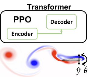
Figure 1. Sketch of DRL framework and data flow. The arrows indicate the control sequence. Before the active learning process, the policy net is first pretrained by the expert data (selected sinusoidal motion) as an imitation learning. In each episode, the agent enquires about the states via observation $o$ from 10 parallel simulation environments where the foil is free to heave and pitch in the uniform inflow. Then the agent sends actions $a$ ($\hat {V}_{\theta }$, $\hat {V}_y$) adjusted by $\hat {\mathcal {L}}$. We implement the XML-RPC (extensible markup language remote procedure call) protocol to enable cross-platform communication between the environment (computational fluid dynamics (CFD) solver) and DRL agent (Python).

Compared with the traditional RL tasks, the foil trajectory planning problem entails overcoming domain-specific obstacles, such as vast exploration spaces and multiobjective preferences.

The vast exploration spaces refer to the wide range of possible trajectories and motion patterns that the flapping foil can adopt within the fluid environment. This space is vast because there are numerous parameters and variables that can be adjusted to influence the motion of the foil, such as the amplitude and frequency of the flapping motion. The significant challenge to the algorithm's exploration arises from the tendency for extensive and often fruitless searches within the vast exploration spaces, which lack meaningful trajectories.

In the context of the foil trajectory planning task, the ways to evaluate the motion pattern are diverse. Therefore, the reward function should be designed to combine multiple objectives, such as maximizing thrust, minimizing energy consumption and achieving stability (Esfahani, Karbasian & Kim Reference Esfahani, Karbasian and Kim2019; Liu et al. Reference Liu, Bhattacharjee, Tian, Young, Ray and Lai2019). However, foil motion planning often involves multiple conflicting objectives (Marler & Arora Reference Marler and Arora2004). Balancing these objectives adds complexity to the exploration space, as different motion patterns may be required to optimize each goal. To address these challenges, we employ a PPO-based algorithm (Schulman et al. Reference Schulman, Wolski, Dhariwal, Radford and Klimov2017) combined with a transformer architecture (Vaswani et al. Reference Vaswani, Shazeer, Parmar, Uszkoreit, Jones, Gomez, Kaiser and Polosukhin2017). Since limited environmental data (e.g. force, pressure on the foil) can be obtained in real-world situations, we formulate this issue as a POMDP, effectively addressed through our transformer architecture implementation. In the following, we emphasize the primary elements of our DRL framework.

PPO algorithm. The PPO algorithm is a popular model-free DRL algorithm used in machine learning and robotics for solving complex decision-making tasks (Raffin et al. Reference Raffin, Hill, Gleave, Kanervisto, Ernestus and Dormann2021; Mock & Muknahallipatna Reference Mock and Muknahallipatna2023). It gains recognition for its stability and effectiveness. The PPO is a policy optimization algorithm that belongs to the family of policy gradient methods. This family of methods utilizes the gradient of expect reward to iteratively optimize policy.

One of the strengths of PPO is its stability in training. The PPO is robust as an efficient approximation of the trust region optimization approach, which promises reliable policy improvement in noisy environments (Zhang et al. Reference Zhang, Chen, Xiao, Li, Liu, Boning and Hsieh2020). The PPO employs clipping to ensure that policy updates are not too drastic, thus approximately operating within a trust region, which defines a boundary for how much the policy can change in each iteration, which helps prevent overly aggressive policy updates, contributing to the algorithm's stability.

In addition, the aforementioned strength of the PPO algorithm also facilitates support for large-scale parallel training (Yu et al. Reference Yu, Velu, Vinitsky, Gao, Wang, Bayen and Wu2022). In parallel training, multiple agents are trained simultaneously on different batches of data. This can significantly accelerate the training process, but it can also lead to instability, since the policies of different agents usually diverge from each other. This divergence leads to unstable policy update, which further hurts the performance of the algorithm. Fortunately, this risk could be mitigated by the clipping technique used in the PPO, making it a good choice for large-scale parallel training. With the large-scale parallel training, more data can be collected in a shorter time, essential for long-episodic and high-dimensional tasks (Berner et al. Reference Berner2019). It is noted that we applied parallel simulation environments in our study, which significantly speed up the training process.

As the trajectories in the context of foil motion planning are longer than common RL tasks, our method faces the problem of credit assignment. The credit assignment problem pertains to the fundamental challenge of attributing the consequences of actions taken by an agent to the responsible decisions or states that preceded those outcomes. It is particularly salient in scenarios where the temporal gap between actions and rewards is substantial. In order to address this issue effectively, we integrate generalized advantage estimation (GAE) (Schulman et al. Reference Schulman, Wolski, Dhariwal, Radford and Klimov2017) into the PPO algorithm to assist in long-term credit assignment, thereby improving the algorithm's performance and data efficiency. This approach has proven favourable for addressing high-dimensional continuous control problems, including the flapping foil problem studied in our current research. The GAE is a pivotal technique in the field of RL. Its core concept lies in estimating the advantage function, denoted as $A(s, a)$. The advantage function quantifies the advantage of choosing a particular action $a$ in a given state $s$ over following the current policy. Mathematically, it is calculated as the difference between the expected cumulative reward, known as the action-value function $Q(s, a)$, and the value function $V(s)$. In other words, it can be expressed as $A(s, a) = Q(s, a) - V(s)$. The use of the advantage function allows us to measure the value of each action, aiding in more precise and effective credit assignment over extended time horizons. However, calculating the advantage function with only one time step return is unstable. The GAE computes the advantage estimate for each time step in an episode by considering a combination of one-step and multistep returns. It combines the advantages from different time scales to provide a more comprehensive view of the advantage function. The GAE introduces a parameter $\lambda$ that controls the degree of generalization across different time steps. By adjusting $\lambda$, you can emphasize more recent rewards or place greater weight on long-term rewards in the advantage estimation, which stabilize the learning process. The formula for GAE with $\lambda$ is as follows:

(2.10)\begin{equation} \text{GAE}(\lambda, t) = (1 - \lambda) \sum_{n=1}^{\infty}(\lambda^n\delta_{t+n-1}), \end{equation}

where $\delta _{t+n-1}$ is the $n$-step advantage at time step $t+n-1$. In addition, PPO is known for being relatively sample-efficient compared with some other RL algorithms. It can learn from fewer interactions with the environment, which can be crucial in situations where collecting data is expensive or time consuming.

The PPO follows the actor–critic framework in RL. The actor ${\rm \pi} (a\,|\,o,b)$, parameterized as $\theta$, interacts with the environment, while the critic $V(s)$, parameterized as $\phi$, predicts the onward cumulative reward. For the actor, PPO maximizes a clip objective to penalize changes to the policy that move $r_{t}(\theta )$ far away from the old policy,

(2.11)\begin{equation} L_{actor}(\theta)=\hat{\mathbb{E}}_{t}[\min (r_{t}(\theta) \hat{A}_{t}, \operatorname{clip}(r_{t}(\theta), 1-\epsilon, 1+\epsilon) \hat{A}_{t})], \end{equation}

where $r_{t}(\theta )={{\rm \pi} _{\theta }(a_{t} \mid s_{t})}/{{\rm \pi} _{\theta _{old}}(a_{t} \mid s_{t})}$ denote the probability ratio, $\epsilon$ is a hyperparameter to constrain the change of policy and $A_t$ is the advantage to reduce policy gradient variance (Sutton & Barto Reference Sutton and Barto2018). The clip function is defined as follows:

(2.12)\begin{equation} \operatorname{clip}(x, l, u) = \begin{cases} u, & x>u\\ x, & l\le x \le u\\ l, & x< l \end{cases}. \end{equation}

For the critic, PPO minimizes the temporal difference loss as follows:

(2.13)\begin{equation} L_{critic}(\phi) = r_{t}+\gamma V(s_{t+1};\phi)-V(s_{t};\phi). \end{equation}

Therefore, the learning objective for PPO is defined as follows:

(2.14)\begin{equation} L(\theta, \phi) = L_{critic}(\phi) + L_{actor}(\theta). \end{equation}

Transformer. As POMDP problems assume that the agent does not have full information about the state of the environment, the agent is required to maintain a belief state over the hidden state of the environment. This can be thought of as a summary of the agent's knowledge about the state of environment. The process of maintaining a belief state over the states necessitates the information of the previous state. Therefore, maintaining a belief state requires the model has the ability to model the time-dependent behaviour (Ni, Eysenbach & Salakhutdinov Reference Ni, Eysenbach and Salakhutdinov2022).

There are two widely applied neural network architectures to model the time-dependent behaviour. Recurrent neural networks (RNNs) (Medsker & Jain Reference Medsker and Jain2001) are a type of neural network that have the ability to model long-term dependencies in data. The RNNs have a recurrent hidden state, which allows them to learn how to model the sequential relationships between the data points. Another one is the transformer architecture (Vaswani et al. Reference Vaswani, Shazeer, Parmar, Uszkoreit, Jones, Gomez, Kaiser and Polosukhin2017) which is a deep learning model that has revolutionized sequence modelling, particularly in natural language processing (NLP) and beyond (Gillioz et al. Reference Gillioz, Casas, Mugellini and Abou Khaled2020; Khan et al. Reference Khan, Naseer, Hayat, Zamir, Khan and Shah2022). Its core innovation lies in its ability to efficiently capture long-range dependencies in sequences through self-attention mechanisms, enabling parallel processing and scalability.

In the context of POMDP problems, RNNs can be used to learn the belief state of the agent. The RNN can be trained on a dataset of past observations and actions, and the agent's belief state can be initialized to the output of the RNN. The agent can then use the RNN to update its belief state at each time step based on its new observation and its current action. However, a notable limitation of RNNs lies in their inherent sequential processing paradigm. RNNs, by design, operate sequentially, processing input data one time step at a time. This sequential nature can present challenges when dealing with lengthy sequences, as it results in linearly increasing computation time proportional to the sequence length. Consequently, for tasks characterized by extensive temporal dependencies or extended input sequences, RNNs may suffer from slower training and inference times. Furthermore, RNNs are susceptible to the vanishing gradient problem when confronted with prolonged sequences, potentially impeding their capacity to effectively capture long-range dependencies. In contrast, the transformer architecture has proven highly parallelizable, enabling the efficient processing of sequences in parallel, a significant departure from the sequential nature of recurrent neural networks. This parallelism contributes to the model's superior scalability and faster training times, making it particularly appealing for handling long sequences and large datasets (Vaswani et al. Reference Vaswani, Shazeer, Parmar, Uszkoreit, Jones, Gomez, Kaiser and Polosukhin2017). This advantage becomes particularly pertinent in applications where the modelling of extensive temporal relationships is imperative.

In order to effectively model the time-dependent behaviour of foil flapping, we employ the transformer architecture, which has been demonstrated to excel in capturing long-term interactions and supporting high training throughput (Brown et al. Reference Brown2020; Esslinger, Platt & Amato Reference Esslinger, Platt and Amato2022). At the heart of the transformer is the self-attention mechanism, which allows each element in the input sequence to attend to all other elements, capturing complex contextual relationships. The self-attention mechanism computes weighted sums of all elements in the sequence, with weights determined dynamically for each element. This attention mechanism is computed in parallel for all elements, leading to highly efficient and scalable processing. The self-attention mechanism can be expressed by the following equation:

(2.15) \begin{equation} \text{Attention}(\boldsymbol{\mathsf{Q}},\boldsymbol{\mathsf{K}},\boldsymbol{\mathsf{V}}) =\text{softmax}\left(\frac{\boldsymbol{\mathsf{Q}}\boldsymbol{\mathsf{K}}^{T}}{\sqrt{d_{k}}}\right)\boldsymbol{\mathsf{V}}, \end{equation}

where $\boldsymbol{\mathsf{Q}}, \boldsymbol{\mathsf{K}}, \boldsymbol{\mathsf{V}}$ are vectors of queries, keys and values, respectively, which are learned during training, and $d_k$ is the dimension of $\boldsymbol{\mathsf{Q}}$ and $\boldsymbol{\mathsf{K}}$. In self-attentions, $\boldsymbol{\mathsf{Q}}, \boldsymbol{\mathsf{K}}, \boldsymbol{\mathsf{V}}$ share the same set of parameters. The attention mechanism allows for the estimation of $P(\kern 1.5pt\boldsymbol {y}\mid \boldsymbol {x})$ or $P(\kern0.7pt y_n\mid x_1, \ldots,x_n)$ without the need for recursive processes, as in RNNs, which results in higher computational efficiency and long-term interaction modelling ability.

Our customized transformer architecture uses the history sequence as the belief about the state, which comprises two primary components: a two-layer encoder and a linear layer as the decoder. Each encoder features a self-attention structure and a feed-forward neural network layer. The self-attention structure incorporates two attention heads, a hidden state dimension of 32, and a query dimension of 128.

Pretraining on expert demonstration. The foil action's cause-and-effect relationship is non-instantaneous and the complete motion pattern consists of thousands of steps. This vast policy space enables the potential discovery of superior foil motion control policies. However, the exponentially expanding exploration space as a function of the simulation length poses challenges to the learning performance. Although the PPO algorithm has mitigated this problem, we find that it still struggles to explore in the exploration space.

To address the substantial exploration space, we use a pretrained model, imitated from sinusoidal expert policies, as an initial starting point in the high-value subspace of the overall policy space. We chose 20 expert policies on the Pareto frontier in § 3.2. We then collected 10 trajectories using each expert policy, ensuring that the trajectories span a diverse range of expert policies and performance outcomes. These trajectories serve as a valuable dataset for fine-tuning our pretrained model using RL techniques. Note that the pretraining differs from imitation learning, because these trajectories are a sample from the sine policies lying on the Pareto frontier. The use of this pretrained model prevents unnecessary and meaningless exploration in the vast exploration space, leveraging the knowledge captured from expert policies while still enabling exploration beyond their capabilities. The learning objective of the pretraining is defined as follows:

(2.16)\begin{equation} L_{pretrain}(\theta) = \mathbb{E}_{s, \hat{a}\sim \mathcal{D}}[(a-{\rm \pi}(s))^2], \end{equation}

where state $s$ and the expert action $\hat {a}$ are sampled from the buffer storing the collected expert trajectories.

Diverse reward functions. The foil motion optimization objectives are the efficiency coefficient and the thrust coefficient, thus designing diverse reward functions to boost the diversity of motion patterns is essential. The reward function applied in the present work is

(2.17)\begin{equation} r_t=\beta_C \,\text{clip}(C_T^t, -C_{T}^{m}, C_{T}^{m}) - \beta_{\mathcal{P}}\, \text{clip}(C_{\mathcal{P}}^t, - C_{\mathcal{P}}^{m}, C_{\mathcal{P}}^{m}) \end{equation}

to balance the maximization of thrust and energy consumption of foil motion. Optimizing the cumulative reward is equivalent to integrating the two terms in the equation with respect to time. The integration of the first terms in the equation with respect to time is an approximation of propulsive impulse while the integration of the second terms in the equation with respect to time is an approximation of energy consumption. Therefore, this reward function encourages the foil to find a policy to maximize the thrust and minimize energy consumption. The clip parameters $C_{T}^{m}$, $C_{\mathcal {P}}^{m}$ alleviate extreme value of $C_T$ and $C_{\mathcal {P}}$, and linear weight $\beta _C, \beta _P$ balance the importance between thrust and energy consumption. The parameter tuple $(\beta _C$, $\beta _{\mathcal {P}}$, $C_T^m$, $C_{\mathcal {P}}^m)$ describes a specific reward function, which is initialized as $(0.1, {1}/{3000}, 10, 3000)$, respectively.

Training pipeline. To enhance data interaction throughput, we employ 10 parallel simulations, serving as the environment to interact with the transformer agent to minimize training time. Communication sequences and data flow are shown in figure 1. Agents are initialized from a fully developed simulation in which the foil remains stationary and void of DRL interference, ensuring a stable vortex shedding state at the onset of training. The pretrained transformer receives 24 observation signals, normalized to $[0,1]$, and outputs normalized rotational and vertical velocity, $\hat {V}_\theta$ and $\hat {V}_y$. These output actions are then scaled by $\hat {\mathcal {L}}$ for amplitude adjustment. Initialized at $[0.5,0.5]$, $\hat {\mathcal {L}}$ remains constant throughout training, and its effects will be discussed in § 3.2. The interactions and updates will be repeated at every time step between agents and the environment.

Our experiments employed the PPO algorithm within the foil scenario, using the following hyperparameters: we utilized a batch size of 256, and set the critic's learning rate at 0.001 and the actor's learning rate at 0.0001. The context length was 50 with a network configuration of two layers, two attention heads and an embedding dimension of 32. Our RL parameters included a discount factor (gamma) of 0.9, 10 PPO inner epochs, a PPO clipping value of 0.2 and an entropy coefficient of 0.01. Additionally, we employed a gradient clipping norm of 0.5 and a GAE lambda of 0.9. For the expert policy pretraining, we use the offline data from sine policies lying on the Pareto frontier discussed in § 3.2. The pseudocode is shown in Algorithm 1.

Algorithm 1 The DRL-based foil non-parametric path planning with PPO.

For reproducibility, we standardized our seed values across the board: neural network; numpy; and random seeds were all set to unity. Our training process was executed over 200 episodes, with evaluations occurring every 50 episodes. Model checkpoints were saved at intervals of two episodes, and rendering was disabled for the duration of training. Our experiments are conducted on a server with 2 Nvidia A100 GPU and AMD EPYC 7742 CPU, and each experiment lasts for around 13 h.

3. Results and discussion

We divide this section into three parts, each designed to examine a particular aspect of the DRL-controlled flapping foil performance: (i) the effectiveness of the proposed DRL framework, (ii) the enhanced performance of the DRL optimized trajectory compared with sinusoidal motions and (iii) physical insight on the benefit of DRL optimization.

3.1. Whether it can flap: the DRL training process of different agents

To demonstrate the effectiveness and efficiency of the proposed learning framework for flapping foil problems, we compare the reward over 200 training episodes (set $(\beta _C, \beta _{\mathcal {P}}, C_T^m, C_{\mathcal {P}}^m) = (0.1, 1/3000, 10, 3000)$ in (B1)) for selected different combinations of RL algorithms and neural network (NN) structures, including RNN+soft actor–critic (SAC), multilayer perceptron (MLP)+PPO and transformer+PPO.

To ensure fair comparison, we apply the same environment parameters for all algorithms, including reward function parameter tuple as $(\beta _C, \beta _{\mathcal {P}}, C_T^m, C_{\mathcal {P}}^m) = (0.1, 1/3000, 10, 3000)$. However, different training parameters are selected for each baseline algorithms to guarantee convergence as follows.

  1. (i) Transformer+PPO (TP) adopts the training setting already described in 2.3.

  2. (ii) RNN+SAC. The learning rates for the actor and critic networks were set to 0.003 and 0.001, respectively. The value of epsilon $\epsilon$, crucial for exploration–exploitation balance, started at 0.5 and decayed to 0.05. The batch size was set to 256. A clipping parameter of 0.2 was used to mitigate exploding gradients. The learning frequency was set to 1. The networks comprised two hidden layers each with 64 hidden state units. A Gaussian policy was employed for action selection. Training was conducted over 200 episodes. Entropy tuning was enabled. Target networks were updated every 30 steps. The capacity of the replay buffer was 10 000. Lastly, the target entropy ratio was set to 0.7. These settings were chosen empirically to ensure effective policy learning while maintaining a balance between exploration and exploitation, stability and computational efficiency.

  3. (iii) MLP+PPO. Our actor and critic use the same MLP network architecture as backbone, which consists of three hidden layers and the hidden state size in each layer is 32. The input dimension of MLP depends on the input history time steps as $\textrm {dim}_{input} = \textrm {dim}_{obs}\times \textrm {steps}$. We utilized a batch size of 256, and set the critic's learning rate at 0.001 and the actor's learning rate at 0.0001. Our RL parameters included a discount factor (gamma) of 0.9, 10 PPO inner epochs, a PPO clipping value of 0.2 and an entropy coefficient of 0.01. Additionally, we employed a gradient clipping norm of 0.5 and a GAE lambda of 0.9.

The comparison result is shown in figure 2. Figure 2(a) shows different learning trends that each framework manages to optimize foil flapping motion. The performance of the RNN+SAC agent (depicted in blue) is notably below par. It commences its training with the lowest recorded initial reward of $-750$, a stark contrast to the other agents. Soon after, it experiences a significant drop in reward, descending into a lower reward range. Over the course of training, the RNN+SAC agent makes efforts to enhance its performance by aiming for higher rewards and learning from formal training episodes. However, its reward trajectory demonstrates large oscillations, consistently hovering around the initial starting point with substantial variance, as indicated by the shaded blue region in the plot.

Figure 2. (a) Reward over 200 episodes of different combinations of RL algorithms and NN structures, and the parameters in the reward function are selected as $(\beta _C, \beta _{\mathcal {P}}, C_T^m, C_{\mathcal {P}}^m) = (0.1, 1/3000, 10, 3000)$. The solid line and shadow represent the mean and variance of three repeated training results, respectively. The inset $C_T$ and $\eta$ plots are selected for the TPPT agent. Note that the agents of MLP+PPO 1 and MLP+PPO 50 have the same NN structure but use the current observation or 50 history data collection as the state, respectively. (b) From left to right: the mean wake velocity profiles; instantaneous vorticity magnitude; the time traces (same time interval of 1) of actions $(\hat {V}_y, \hat {V}_{\theta })$; and forces coefficients $(C_T, C_L)$ for three cases denoted as red dots in panel (a) where (A) is the 14th episode, $\bar {C}_T = 1.93$ and $\eta = 0.12$; (B) is the 104th episode, $\bar {C}_T = 4.0$ and $\eta = 0.13$; (C) is the 182th episode, $\bar {C}_T = 3.52$ and $\eta = 0.16$.

In contrast, the two agents MLP+PPO, represented by the purple and red lines, exhibit distinct patterns. Both MLP+PPO agents start their training with relatively high initial rewards of $-$400. The MLP+PPO 1 agent (purple) gradually approaches a reward of $-$100 by episode 200, showing slow but steady progress with minimal variance (indicated by the purple shadow). Meanwhile, the MLP+PPO 50 agent (red) makes rapid progress within the first 30 episodes, reaching a reward of 0 at episode 50. This ascent is characterized by a steady rate of increase, although it has relatively high variance (shown by the red shadow), compared with the MLP+PPO 1 agent.

On a different note, the two TP agents (depicted in green and yellow) excel in learning the oscillatory flapping motion, achieving the highest rewards among the selected algorithms. The TP agent initialized with a random policy (yellow) exhibits rapid learning, with its reward rapidly ascending and surpassing other agents before episode 60. However, around episode 140, it experiences a decline in reward, eventually reaching zero. This descent is accompanied by pronounced oscillations in variance, denoted by the yellow shadow. In contrast, the pretraining TP agent (TPPT) quickly reaches its maximum convergence reward of 100 before episode 40. It exhibits minimal fluctuations with reduced variance (as indicated by the green shadow) throughout repeated training processes, in contrast to the TP agent initialized with a random policy.

To visually illustrate the enhanced process and the convergence of hydrodynamic performance with respect to $\bar {C}_T$ and $\eta$, we have included subfigures for the TPPT agent. In the process of optimizing $\bar {C}_T$ and $\eta$, thrust shows a notable improvement increase before the 50th episode, followed by oscillations and a subsequent decline to a relatively stable value around 3.5. In contrast, efficiency experiences an initial rapid increase prior to the 50th episode, followed by a steady rise towards its convergence value of 0.15.

In figure 2, we have chosen three specific cases (indicated by red dots) to elucidate the evolution of the TPPT agent, and we have plotted their mean wake velocity profiles, instantaneous vorticity, as well as the time history of actions and forces (as shown in figure 2b from left to right).

Starting with case A, it is evident that the action curves closely resemble a sinusoidal motion with minor oscillations. This behaviour can be attributed to the expert demonstrations provided during the pretraining phase. The hydrodynamic force curves exhibit simple sinusoidal undulation, with the exception of $C_T$, which displays double peak values.

As we transition to case B, the action curves become clearly non-sinusoidal, although they still exhibit oscillatory behaviour. However, they gradually evolve into a phase with sudden changes, spikes and plateaus, resulting in higher spikes and more pronounced rates of change in generated values for both $C_T$ and $C_L$. Notably, $C_T$ exhibits a more pronounced double-peak characteristic with higher values, and the rate of change in $C_L$ becomes more substantial. Similarly, a comparison of mean velocity profiles in the wake between cases A and B reveals the emergence of a stronger jet, indicating that the TPPT agent has learned to achieve a higher $C_T$ for improved hydrodynamic performance. Despite minimal changes in reward during continued training, we observe that in case C, the pitching velocity and its rate of change become smoother, while the heaving velocity still exhibits significant variation. This leads to more moderate, stable and less spiky force profiles, where the double-peak characteristic of $C_T$ weakens with the plateaus becoming evident. Although there is a decrease in $C_T$ from case B to case C, it is worth noting that $\eta$ increases by 23 $\%$ from case B to C, as depicted in figure 2(a).

3.2. How well it flaps: the hydrodynamic outperformance through reward shaping

After showcasing the effectiveness of the TPPT agent, to highlight its superiority in foil trajectory optimization, we compare the hydrodynamic performances of various TPPT agents’ optimized trajectories with the results of a brute-force search for sinusoidal motion in $\bar {C}_T$ and $\eta$. Some of these results also serve as expert policies and initializations for the TPPT agent, as illustrated in figure 3.

Figure 3. Scatters of $\bar {C}_T$ and $\eta$ for sinusoidal (blue) and TPPT agent (red) optimized motions. Note that the big red dots have different rewards tuples and the small red dots are acquired by adjusting $\hat {\mathcal {L}}$ after the training is finished. The inset figures plot instantaneous vorticity, the $\hat {V}_y$ (red) and $\hat {V}_{\theta }$ (blue) time trace of the selected three cases. In scenario I, $\bar {C}_T = 0.562$, $\eta = 0.28$, the reward tuple is $(0.08, {1}/{3000}, 8, 3000)$ and $\hat {\mathcal {L}} = [0.49,0.49]$. In Scenario II, $\bar {C}_T = 4.40$, $\eta = 0.184$, the reward tuple is $(0.1, {1}/{3000}, 10, 3000)$ and $\hat {\mathcal {L}} = [0.5,0.5]$. In Scenario III, $\bar {C}_T = 14.3$, $\eta = 0.14$, reward tuple is $(0.1, {1}/{3000}, 10, 3000)$ and $\hat {\mathcal {L}} = [0.58,0.58]$. In Scenario IV, $\bar {C}_T = 25.7$, $\eta = 0.08$, the reward tuple is $(0.1, {1}/{3000}, 30, 3000)$ and the $\hat {\mathcal {L}} = [0.5,0.5]$.

Figure 3 presents a visual representation of the results obtained from brute-force search, indicated by small blue dots, alongside the cases trained using TPPT agents. In a brute-force search, we systematically explored the parameter space associated with sinusoidal flapping motion, defined by the ranges $Sr \in [0.1, 0.4]$, $h_0 \in [0.1, 0.6]$, $\theta _0 \in [5^{\circ }, 70^{\circ }]$ and $\phi \in [0^{\circ }, 180^{\circ }]$. It's important to note that, out of the 3156 trials conducted in the brute-force search, only cases resulting in positive values for both $\bar {C}_T$ and $\eta$ are displayed in figure 3 for clarity.

Within figure 3, the small blue dots are distributed in an area where the highest $\bar {C}_T$ and $\eta$ values are 26.683 and 0.224, respectively. Their spatial distribution forms a triangular pattern with a subtly curved front sideline. Most of these blue dots cluster in the region characterized by high values of $\eta$, and as the value of $C_T$ increases, the density of the dots gradually decreases. The curved front sideline distinctly outlines a Pareto front, a well-recognized reference line in multiobjective optimization (Marler & Arora Reference Marler and Arora2010; Preparata & Shamos Reference Preparata and Shamos2012). In the context of multiobjective optimization, any trained results that surpass the Pareto front are considered optimized ones.

Among the results of TPPT-trained cases, represented by both large and small red dots, two TPPT agents with different reward tuples (large red dots) and five evolved TPPT agents with varying $\hat {\mathcal {L}}$ (small red dots) achieved results clearly superior to the Pareto front established by the brute-force search. It is important to highlight that, within the parameters of our simulation setting (with $Re = 1173$), the highest efficiency achieved among the brute-force search results stands at 0.224, clearly lower than the results of over 0.7 acquired in the experiments by Streitlien & Barrett (Reference Streitlien and Barrett1998) and Hover & Triantafyllou (Reference Hover and Triantafyllou2003) at high Reynolds number $Re$ over 10 000. However, it is important to note that the efficiency $\eta$ of the flapping foil is highly influenced by the Reynolds number and shape of the foil. For instance, Schouveiler, Hover & Triantafyllou (Reference Schouveiler, Hover and Triantafyllou2005) observed a peak efficiency of $\eta = 0.8$ at $Re = 40\,000$, while Dong, Mittal & Najjar (Reference Dong, Mittal and Najjar2006) reported a maximum efficiency of $\eta = 0.18$ at $Re = 200$ for a rigid flapping panel. Moreover, Buchholz & Smits (Reference Buchholz and Smits2008) mentions that increasing the Reynolds number from 100 to 400 would lead to the propulsive efficiency of the pitching panel increasing approximately twice because there is correspondingly substantial shear drag under the relatively low Reynolds number (Dong et al. Reference Dong, Mittal and Najjar2006). Therefore, this study focuses primarily on motion optimization instead of Reynolds number, which we will discuss in subsequent sections.

We have selected four scenarios to clearly illustrate the improvements in $\bar {C}_T$ and $\eta$ introduced by changes in actions, and we have plotted their instantaneous vorticity and the time history of actions. In the first scenario (Scenario I), the primary objective is to optimize and enhance the flapping efficiency $\eta$ by reducing $\beta _C$ to 0.08. On the contrary, Scenarios II and III aim to strike a balance in optimizing objectives between $\bar {C}_T$ and $\eta$. Scenario III has slightly higher action limits ($\hat {\mathcal {L}}$), allowing it to achieve a higher $\bar {C}_T$ without a significant compromise in $\eta$. In contrast, Scenario IV prioritizes thrust optimization by increasing $C_T^m$ in its reward tuple, emphasizing thrust production.

In Scenario I, the action curves resemble sinusoidal motion, but the mean value of heaving velocity deviates significantly from zero. On the other hand, Scenarios II to IV exhibit non-sinusoidal actions, sharing similar features with the case C in § 3.1. In Scenario II, $\bar {C}_T$ and $\eta$ improve compared with case C in § 3.1, but the action history differs due to an extended total training episode.

Comparing Scenario II with Scenario III, where the $\hat {\mathcal {L}}$ value is increased, the $\bar {C}_T$ of Scenario III experiences a remarkable enhancement, with increased amplitude of $\hat {V}_{\theta }$ and $\hat {V}_y$, along with the appearance of spikes and plateaus. Compared with Scenario II, Scenario IV places greater emphasis on optimization $\bar {C}_T$ by increasing $C_T^m$, further improving $\bar {C}_T$. In Scenario IV, the actions evolve into more complex forms with higher spikes and greater velocity variation at higher action frequencies. Notably, we observed that from Scenario I to Scenario IV, the amplitude of the velocity of the pitching actions increases as the agent's corresponding $\bar {C}_T$ is enhanced. It is important to note that although $\eta$ decreases from Scenario I to Scenario IV, the overall hydrodynamic performance still surpasses the Pareto front of the Brute Force search.

3.3. Why it flaps better: the physical insight of DRL optimization strategy

To illuminate the underlying mechanism behind the improvement in flapping performance by the TPPT agent, we conduct an analysis and present plots in figures 4, 5, 6 and 7. These figures provide insights into the vorticity (figures 4$a$,$b$, 6$a$,$b$ and 7$a$,$b$), pressure distributions around the foil (figures 4$c$,$e$, 6$c$,$e$ and 7$c$,$e$), and the time history of actions and forces (figures 4$d$,$f$, 6$d$,$f$ and 7$d$,$f$) for Scenario I, Scenario III and Scenario IV (as shown in figure 3), along with their statistically equivalent sinusoidal motion counterparts. In our study, the sinusoidal counterparts share statistically identical velocity amplitudes for both heaving and pitching motions, Strouhal number $S_r$ and phase shift $\phi$, between the two motions. These consistent amplitudes are obtained by multiplying the standard deviation of the TPPT-controlled motion by the square root of two. Additionally, the phase shift for pitching and heaving motion is determined by subtracting the unwrapped value obtained after applying the Hilbert transformation. Lastly, the statistical value of $S_r$ is straightforwardly calculated by dividing the velocity circle by the non-dimensional time.

Figure 4. Instantaneous vorticity, pressure distributions and time trace of action and force over three vortex shedding periods for (a) the TPPT Scenario I and (b) its statistically equivalent sinusoidal motion. (cf) Four foil posture moments are selected to show complete pressure distribution change along the foil (the blue arrow represents the negative pressure region, while the red arrow represents the positive pressure region). For better visualization, the foil shown here is NACA 0020 instead of NACA 0016, and the $C_p$ is scaled to 1/2 from its original value.

Figure 5. (a) Vorticity plot of one entire vortex shedding and motion period of TPPT Scenario I. (b) Vorticity plot of one entire vortex shedding and motion period of sinusoidal counterpart. (c) The foil posture versus its pitching velocity for TPPT Scenario I. The blue quivers represent hydrodynamic force at that moment. (d) The foil posture versus its pitching velocity for sinusoidal counterpart of Scenario I. The blue quivers represent forces’ magnitude and direction at that moment. (e) Time trace of motion ($\hat {V}_{\theta }$ and $\hat {V}_y$) and power coefficient ($C_{\mathcal {P}}$) for (i) TPPT Scenario I and (ii) its statistically equivalent sinusoidal motion.

Figure 6. Instantaneous vorticity, pressure distributions, mean wake velocity at three chord lengths away from trailing edge, time trace of action and force over four vortex shedding periods for (a) TPPT Scenario IV and (b) its statistically equivalent sinusoidal motion. (cf) Four foil posture moments are selected to show complete pressure distribution change along the foil (the blue arrow represents the negative pressure region, while the red arrow represents the positive pressure region). For better visualization, the foil shown here is NACA 0020 instead of NACA 0016, and the $C_p$ is scaled to 1/10 from its original value. The plots of foil posture versus pitching velocity for (g) Scenario IV and (h) its counterpart are shown here. Note that the blue quivers represent scaled forces’ magnitude and direction at that moment.

Figure 7. Instantaneous vorticity, pressure distributions and time trace of action and force over two vortex shedding periods for (a) TPPT Scenario III and (b) its statistically equivalent sinusoidal motion. (cf) Four foil posture moments are selected to show complete pressure distribution change along the foil (the blue arrow represents the negative pressure region, while the red arrow represents the positive pressure region). For better visualization, the foil shown here is NACA 0020 instead of NACA 0016, and the $C_p$ is scaled to 1/10 from its original value.

In the three selected scenarios,

  1. (i) Scenario I (emphasizing on $\eta$) focuses on maximizing flapping efficiency while ensuring thrust remains substantial by slightly decreasing $\beta _C$ in the reward tuple;

  2. (ii) Scenario III (balancing between $\eta$ and $C_T$) achieves an equilibrium in the optimization process, giving equal consideration to both $\eta$ and $C_T$ by slightly increasing $\hat {\mathcal {L}}$;

  3. (iii) Scenario IV (emphasizing on $C_T$) prioritizes maximizing thrust by significantly increasing $C_T^m$ in the reward tuple.

Figure 4 presents the comparison between Scenario I (figure 4a) and its equivalent sinusoidal motion counterpart (figure 4b). When comparing the instantaneous vorticity in figure 4(a,b) (also depicted in figure 5a,b), it becomes evident that despite sharing the same $S_r$, the TPPT-controlled Scenario I exhibits a lower vortex shedding frequency. However, the strength of the vortex pairs is more pronounced in the far wake of the foil for this scenario. This difference is also reflected in the comparison of thrust coefficient ($C_T$), lift coefficient ($C_L$) (as shown in figure 4d,e), and power coefficient ($C_P$) (depicted in figure 5). In figure 4, both scenarios exhibit similar pressure distributions around the foils. However, the TPPT-controlled Scenario I outperforms its sinusoidal counterpart, with a peak $C_T$ of 2.67 compared with 1.24 and a mean $C_T$ of 0.719 compared with 0.416.

To clearly understand the enhancement, we plot the instantaneous power coefficient in figure 5. The TPPT-controlled Scenario I also outperforms its sinusoidal counterpart. Although it has a higher peak power coefficient ($C_P$), with a mean $C_P$ of 29.8, it remains lower than its counterpart, which has a mean $C_P$ of 37.2. This performance pattern aligns with the optimization goal outlined in (2.4), where the TPPT-controlled Scenario I aims to achieve a higher mean thrust while maintaining a lower power coefficient by decreasing vortex shedding frequency, ultimately optimizing its flapping efficiency.

Figure 6 presents the comparison between Scenario IV (figure 6a) and its equivalent sinusoidal motion counterpart (figure 6b). When comparing the instantaneous vorticity in figure 6(a,b), it shows a more regulated vorticity pattern behind the foil of the DRL optimized motion. In addition, from figure 6(c,e) of the pressure distribution along the foil at four instants, we can quantitatively observe the effects of a strengthened separated wake through pressure distributions around the foil. Depending on the orientation of the foil surface, the pressure acting perpendicularly to the surface can either contribute to thrust or drag forces (Lucas, Lauder & Tytell Reference Lucas, Lauder and Tytell2020). When comparing the values of positive and negative pressure around the foil trailing edge in D2 and D3 moments with those in S2 and S3, it is evident that they are significantly increased. This increase in pressure functions to directly boost $C_T$. Notably, the D3 moment, characterized by the maximum acceleration, stands out in this regard.

In the time traces of $C_T$ and $C_L$ (figure 6$d$,$f$), a distinct difference becomes evident. Scenario IV displays a $C_T$ curve that reaches a higher peak value and exhibits slower cycles, resulting in an impressive $\bar {C}_T$ value of 25.7. In contrast, its counterpart achieves a relatively modest $\bar {C}_T$ of 16.5.

To further elucidate the thrust superiority of Scenario IV, we present a comparison of mean wake velocity profiles and pitching velocity versus its forces in figure 6. At three chord lengths away, Scenario IV exhibits three distinct peaks in mean wake velocities, with larger peak values compared with its counterpart. These mean wake velocity profiles align with the vorticity plot, highlighting Scenario IV's advantage in generating a more regular backward shed vortex, contributing to increased thrust. In contrast, its counterpart experiences complex and irregular vortex shedding, which introduces drag and diminishes thrust. In figure 6(d,f), it is evident that Scenario IV produces less reduced drag force, as evidenced by the fewer backward blue quivers for Scenario IV.

Figure 7 illustrates the comparison between Scenario III (figure 7a) and its equivalent sinusoidal motion counterpart (figure 7b). A pattern reminiscent of Scenario IV emerges, where the positive and negative pressure values surrounding the trailing edge of the foil experience a significant increase during the D3 moments. This phenomenon directly contributes to the enhancement of $C_T$, the mean thrust coefficient. It is noteworthy that the D3 moment coincides with the instance of maximum rate of change in pitching and heaving velocities.

In contrast to Scenarios I and IV, Scenario III adopts a more balanced approach to optimization, aiming for equilibrium between $\bar {C}_T$ and $\eta$. As a result, its actions are positioned at an intermediate point between the two extremes. Consequently, the peak value of $C_T$ achieved in Scenario III falls within the range observed in Scenarios I and IV.

By combining the visualizations of vorticity in figure 7(a,b), pressure distributions around the foil in figure 7(c,e) and the time history of actions and forces in figure 7(d,f) in Scenarios I to IV, we show that under the dual objectives of maximizing $\bar {C}_T$ and minimizing $\eta$, the TPPT agent demonstrates the ability to discern the presence of separated vortices near the foil body through pressure cues. It then actively adjusts its kinematics to exploit these vortices, thereby enhancing the overall hydrodynamic performance. This hypothesis aligns with the notion presented in previous research (Müller et al. Reference Müller, Van Den Heuvel, Stamhuis and Videler1997), suggesting that fish possess the capability to adapt their kinematics to control near-body flow, ultimately leading to improvements in swimming performance.

4. Conclusion

In the present work, our aim is to answer whether the DRL agent can learn a reasonable strategy for complex unsteady fluid control problems such as foil flapping, how well it performs compared with the sinusoidal motion, and if so why the agent can learn better.

By carefully devising the training framework (TPPT in our case) and comparing it with other popular training frameworks (RNN+SAC, MLP+PPO), the agent can outperform the Pareto front, multiobjective optimization baseline, of a brute force search for the sinusoidal motion by taking advantage of the vortex–foil interaction and learning coherent non-parametric trajectories. In addition, by adding expert data as the initialization, the agent can reach convergence rapidly with the highest reward value in a relatively low repeat variance.

Furthermore, with a close look into the wake morphology, instantaneous pressure distribution, mean wake velocity profiles and the time trace of the power coefficient of the foil's trained motion, the agent can adaptively adjust the statistically similar sinusoidal motion, generating stronger vortices and alternating phases between the motions of the foil and shedding vortices, thus leading to an improvement in hydrodynamic performance.

It is noted that in the current work, we select the simulation environment of low mesh density and the Reynolds number for the proof-of-concept demonstration of DRL with unsteady flapping foil flow control. We believe that our result, for the first time, shows the potential of DRL in complex and time-variant flow control, providing a feasible method to reproduce animal-similar flapping motion and solve other complex flow manipulation tasks.

Declaration of interests

The authors report no conflict of interest.

Appendix A

We conducted a series of computations with parameters set to $St=0.25$, $A_c=0.2$, $\theta _0=10^\circ$ and $\phi =180^\circ$ using different mesh densities to validate the accuracy of our simulations and assess mesh density convergence. The results of mesh convergence are presented in figure 8(a). In this figure, the horizontal axis represents the resolution in terms of grid points per chord length, while the vertical axis depicts the values of $C_T$ and $\eta$ obtained from the simulations. It is evident that both $C_T$ and $\eta$ converge as the mesh density increases, affirming the convergence of our simulation results. Considering the trade off between computation time and error control, we selected a mesh density of 32 points per chord length for the present study.

Figure 8. (a) Mesh convergence results of $\bar {C}_T$, $\bar {C}_p$ and $\eta$. Simulation is conducted under $\theta _0 = 10^{\circ }$, $A_C = 0.2$, $\phi = {\rm \pi}$, $S_r = 0.25$. The mesh density is defined by how many grids per foil chord. (b) The comparison result of thrust coefficient neutral line between our simulation and Lagopoulos et al. (Reference Lagopoulos, Weymouth and Ganapathisubramani2019).

To further validate the computational accuracy of our simulations, especially concerning hydrodynamic force coefficients, particularly the thrust coefficient, we conducted a series of simulations using the same parameters as Lagopoulos et al. (Reference Lagopoulos, Weymouth and Ganapathisubramani2019). These simulations covered a range of $S_r$ values within $[0.2, 0.5]$ and scaled pitching amplitudes within $[0.2, 2]$. The comparison results are displayed in figure 8(b). In this figure, the blue line represents the thrust neutral line from the results of Lagopoulos et al. (Reference Lagopoulos, Weymouth and Ganapathisubramani2019), where the corresponding thrust coefficient equals zero. The red dots represent the results of our simulations. Our results closely match those from the referenced study, with minor discrepancies that can be considered negligible given that our primary focus is on optimizing flapping trajectories.

Appendix B

In this section, we manage to enhance the hydrodynamic performance of the foil by incorporating a lift force restriction term into the reward function. The revised reward function is defined as follows:

(B1)\begin{equation} r_t=\beta_C \,\text{clip}(C_T^t, -C_{T}^{m}, C_{T}^{m}) - \beta_{\mathcal{P}}\, \text{clip}(C_{\mathcal{P}}^t, - C_{\mathcal{P}}^{m}, C_{\mathcal{P}}^{m}) - y_{penalty}. \end{equation}

In this revised reward function, the supplementary term serves as a means to mitigate the occurrence of asymmetric vortex shedding. If the current position of the foil deviates significantly from its initial vertical position, a progressively escalating penalty is applied to discourage sustained deviations. This penalty is designed to deter instances of foil spiking and continual deviations in the heaving direction. By doing so, it incentivizes the foil's motion to induce more symmetric vortex shedding patterns towards the rear of the foil, contributing to an overall enhancement of hydrodynamic performance.

The new training results are presented in figure 9 as green dots, while the blue and red dots are the same as those shown in figure 3. Notably, most of the green dots do not surpass the formal TPPT-optimized performance. Only three of the green dots exhibit a slight improvement in efficiency, lightly exceeding the TPPT-optimized performance.

Figure 9. The identical Pareto front as figure 3. Addition of new TPPT training cases (green) of the adding lift force constraining term in the reward function.

Footnotes

These authors contributed equally to this work.

References

Ashraf, I., Wassenbergh, S.V. & Verma, S. 2021 Burst-and-coast swimming is not always energetically beneficial in fish (Hemigrammus bleheri). Bioinspir. Biomim. 16 (1), 016002.CrossRefGoogle Scholar
Barrett, D.S., Triantafyllou, M.S., Yue, D.K.P., Grosenbaugh, M.A. & Wolfgang, M.J. 1999 Drag reduction in fish-like locomotion. J. Fluid Mech. 392, 183212.CrossRefGoogle Scholar
Beal, D.N., Hover, F.S., Triantafyllou, M.S., Liao, J.C. & Lauder, G.V. 2006 Passive propulsion in vortex wakes. J. Fluid Mech. 549, 385402.CrossRefGoogle Scholar
Beattie, C., et al. 2016 Deepmind lab. arXiv:1612.03801Google Scholar
Berner, C., et al. 2019 Dota 2 with large scale deep reinforcement learning, p. 1. arXiv:1912.06680Google Scholar
Brown, T., et al. 2020 Language models are few-shot learners. Adv. Neural Inf. Process. Syst. 33, 18771901.Google Scholar
Buchholz, J.H.J. & Smits, A.J. 2008 The wake structure and thrust performance of a rigid low-aspect-ratio pitching panel. J. Fluid Mech. 603, 331365.CrossRefGoogle ScholarPubMed
Cassandra, A.R. 1998 A survey of POMDP applications. In Working Notes of AAAI 1998 Fall Symposium on Planning with Partially Observable Markov Decision Processes, vol. 1724.Google Scholar
Chin, D.D. & Lentink, D. 2016 Flapping wing aerodynamics: from insects to vertebrates. J. Expl Biol. 219 (7), 920932.CrossRefGoogle ScholarPubMed
Degrave, J., et al. 2022 Magnetic control of tokamak plasmas through deep reinforcement learning. Nature 602 (7897), 414419.CrossRefGoogle ScholarPubMed
Domenici, P. & Blake, R.W. 1997 The kinematics and performance of fish fast-start swimming. J. Expl Biol. 200 (8), 11651178.CrossRefGoogle ScholarPubMed
Dong, H., Mittal, R. & Najjar, F.M. 2006 Wake topology and hydrodynamic performance of low-aspect-ratio flapping foils. J. Fluid Mech. 566, 309343.CrossRefGoogle Scholar
Dusek, J., Kottapalli, A.G.P., Woo, M.E., Asadnia, M., Miao, J., Lang, J.H. & Triantafyllou, M.S. 2012 Development and testing of bio-inspired microelectromechanical pressure sensor arrays for increased situational awareness for marine vehicles. Smart Mater. Struct. 22 (1), 014002.CrossRefGoogle Scholar
Esfahani, M.A., Karbasian, H.R. & Kim, K.C. 2019 Multi-objective optimization of the kinematic parameters of fish-like swimming using a genetic algorithm method. J. Hydrodyn. 31, 333344.CrossRefGoogle Scholar
Esslinger, K., Platt, R. & Amato, C. 2022 Deep transformer q-networks for partially observable reinforcement learning. arXiv:2206.01078Google Scholar
Fan, D., Yang, L., Wang, Z., Triantafyllou, M.S. & Karniadakis, G.E. 2020 Reinforcement learning for bluff body active flow control in experiments and simulations. Proc. Natl Acad. Sci. 117 (42), 2609126098.CrossRefGoogle ScholarPubMed
Fish, F.E. 1993 Power output and propulsive efficiency of swimming bottlenose dolphins (Tursiops truncatus). J. Expl Biol. 185 (1), 179193.CrossRefGoogle Scholar
Flinois, T.L.B. & Morgans, A.S. 2016 Feedback control of unstable flows: a direct modelling approach using the eigensystem realisation algorithm. J. Fluid Mech. 793, 4178.CrossRefGoogle Scholar
Floryan, D., Van Buren, T., Rowley, C.W. & Smits, A.J. 2017 Scaling the propulsive performance of heaving and pitching foils. J. Fluid Mech. 822, 386397.CrossRefGoogle Scholar
Gazzola, M., Argentina, M., Mahadevan, L. 2014 Scaling macroscopic aquatic locomotion. Nat. Phys. 10 (10), 758761.CrossRefGoogle Scholar
Gerhard, J., Pastoor, M., King, R., Noack, B., Dillmann, A., Morzynski, M. & Tadmor, G. 2003 Model-based control of vortex shedding using low-dimensional Galerkin models. In 33rd AIAA Fluid Dynamics Conference and Exhibit, p. 4262.Google Scholar
Gillioz, A., Casas, J., Mugellini, E. & Abou Khaled, O. 2020 Overview of the transformer-based models for NLP tasks. In 2020 15th Conference on Computer Science and Information Systems (FedCSIS), pp. 179–183. IEEE.CrossRefGoogle Scholar
Godoy-Diana, R., Aider, J.-L. & Wesfreid, J.E. 2008 Transitions in the wake of a flapping foil. Phys. Rev. E 77 (1), 016308.CrossRefGoogle ScholarPubMed
Guéniat, F., Mathelin, L. & Hussaini, M.Y. 2016 A statistical learning strategy for closed-loop control of fluid flows. Theor. Comput. Fluid Dyn. 30, 497510.CrossRefGoogle Scholar
Hover, F.S. & Triantafyllou, M.S. 2003 Forces on oscillating foils for propulsion and maneuvering. J. Fluids Struct. 17 (1), 163183.Google Scholar
Izraelevitz, J.S. & Triantafyllou, M.S. 2014 Adding in-line motion and model-based optimization offers exceptional force control authority in flapping foils. J. Fluid Mech. 742, 534.CrossRefGoogle Scholar
Jayne, B.C. & Lauder, G.V. 1995 Speed effects on midline kinematics during steady undulatory swimming of largemouth bass, Micropterus salmoides. J. Expl Biol. 198 (2), 585602.CrossRefGoogle Scholar
Khan, S., Naseer, M., Hayat, M., Zamir, S.W., Khan, F.S. & Shah, M. 2022 Transformers in vision: a survey. ACM Comput. Surv. (CSUR) 54 (10s), 141.CrossRefGoogle Scholar
Lagopoulos, N.S., Weymouth, G.D. & Ganapathisubramani, B. 2019 Universal scaling law for drag-to-thrust wake transition in flapping foils. J. Fluid Mech. 872, R1.CrossRefGoogle Scholar
Lagopoulos, N.S., Weymouth, G.D. & Ganapathisubramani, B. 2020 Deflected wake interaction of tandem flapping foils. J. Fluid Mech. 903, A9.CrossRefGoogle Scholar
Li, G., Ashraf, I., François, B., Kolomenskiy, D., Lechenault, F., Godoy-Diana, R., Thiria, B. 2021 Burst-and-coast swimmers optimize gait by adapting unique intrinsic cycle. Commun. Biol. 4 (1), 40.CrossRefGoogle ScholarPubMed
Licht, S., Polidoro, V., Flores, M., Hover, F.S. & Triantafyllou, M.S. 2004 Design and projected performance of a flapping foil AUV. IEEE J. Ocean. Engng 29 (3), 786794.CrossRefGoogle Scholar
Lighthill, J. 1969 Hydromechanics of aquatic animal propulsion. Annu. Rev. Fluid Mech. 1 (1), 413446.CrossRefGoogle Scholar
Lighthill, M.J. 1971 Large-amplitude elongated-body theory of fish locomotion. Proc. R. Soc. Lond. B Biol. Sci. 179 (1055), 125138.Google Scholar
Liu, K., Huang, H.B. & Lu, X.-Y. 2020 Hydrodynamic benefits of intermittent locomotion of a self-propelled flapping plate. Phys. Rev. E 102, 053106.CrossRefGoogle ScholarPubMed
Liu, Z., Bhattacharjee, K.S., Tian, F.-B., Young, J., Ray, T. & Lai, J.C.S. 2019 Kinematic optimization of a flapping foil power generator using a multi-fidelity evolutionary algorithm. Renew. Energy 132, 543557.CrossRefGoogle Scholar
Low, K.H. 2011 Current and future trends of biologically inspired underwater vehicles. In 2011 Defense Science Research Conference and Expo (DSR), pp. 1–8. IEEE.CrossRefGoogle Scholar
Lucas, K.N., Lauder, G.V. & Tytell, E.D. 2020 Airfoil-like mechanics generate thrust on the anterior body of swimming fishes. Proc. Natl Acad. Sci. 117 (19), 1058510592.CrossRefGoogle ScholarPubMed
Luo, B., Liu, D. & Wu, H.-N. 2017 Adaptive constrained optimal control design for data-based nonlinear discrete-time systems with critic-only structure. IEEE Trans. Neural Netw. Learn. Syst. 29 (6), 20992111.CrossRefGoogle ScholarPubMed
Maertens, A.P. & Weymouth, G.D. 2015 Accurate cartesian-grid simulations of near-body flows at intermediate Reynolds numbers. Comput. Meth. Appl. Mech. Engng 283, 106129.CrossRefGoogle Scholar
Marler, R.T. & Arora, J.S. 2004 Survey of multi-objective optimization methods for engineering. Struct. Multidiscipl. Optim. 26, 369395.CrossRefGoogle Scholar
Marler, R.T. & Arora, J.S. 2010 The weighted sum method for multi-objective optimization: new insights. Struct. Multidiscipl. Optim. 41, 853862.CrossRefGoogle Scholar
Medsker, L.R. & Jain, L.C. 2001 Recurrent neural networks. Design Appl. 5 (64–67), 2.Google Scholar
Mock, J.W. & Muknahallipatna, S.S. 2023 A comparison of PPO, TD3 and SAC reinforcement algorithms for quadruped walking gait generation. J. Intell. Learn. Syst. Appl. 15 (1), 3656.Google Scholar
Muhammad, Z., Alam, M.M. & Noack, B.R. 2022 Efficient thrust enhancement by modified pitching motion. J. Fluid Mech. 933, A13.CrossRefGoogle Scholar
Müller, U.K., Van Den Heuvel, B.L.E., Stamhuis, E.J. & Videler, J.J. 1997 Fish foot prints: morphology and energetics of the wake behind a continuously swimming mullet (Chelon labrosus risso). J. Expl Biol. 200 (22), 28932906.CrossRefGoogle Scholar
Newman, J.N. 1977 Marine Hydrodynamics. MIT Press.CrossRefGoogle Scholar
Ni, T., Eysenbach, B. & Salakhutdinov, R. 2022 Recurrent model-free RL can be a strong baseline for many POMDPs. In International Conference on Machine Learning, ICML 2022, 17–23 July 2022, Baltimore, Maryland, USA (ed. K. Chaudhuri, S. Jegelka, L. Song, C. Szepesvári, G. Niu & S. Sabato), Proceedings of Machine Learning Research, vol. 162, pp. 16691–16723. PMLR.Google Scholar
Peng, X.B., Berseth, G. & Van de Panne, M. 2016 Terrain-adaptive locomotion skills using deep reinforcement learning. ACM Trans. Graph. 35 (4), 112.Google Scholar
Preparata, F.P. & Shamos, M.I. 2012 Computational Geometry: An Introduction. Springer Science & Business Media.Google Scholar
Qi, J., et al. 2022 Recent progress in active mechanical metamaterials and construction principles. Adv. Sci. 9 (1), 2102662.CrossRefGoogle ScholarPubMed
Rabault, J., Kuchta, M., Jensen, A., Réglade, U. & Cerardi, N. 2019 Artificial neural networks trained through deep reinforcement learning discover control strategies for active flow control. J. Fluid Mech. 865, 281302.CrossRefGoogle Scholar
Raffin, A., Hill, A., Gleave, A., Kanervisto, A., Ernestus, M. & Dormann, N. 2021 Stable-baselines3: reliable reinforcement learning implementations. J. Machine Learning Res. 22 (1), 1234812355.Google Scholar
Schlanderer, S.C., Weymouth, G.D. & Sandberg, R.D. 2017 The boundary data immersion method for compressible flows with application to aeroacoustics. J. Comput. Phys. 333, 440461.CrossRefGoogle Scholar
Schnipper, T., Andersen, A. & Bohr, T. 2009 Vortex wakes of a flapping foil. J. Fluid Mech. 633, 411423.CrossRefGoogle Scholar
Schouveiler, L., Hover, F.S. & Triantafyllou, M.S. 2005 Performance of flapping foil propulsion. J. Fluids Struct. 20 (7), 949959.CrossRefGoogle Scholar
Schulman, J., Wolski, F., Dhariwal, P., Radford, A. & Klimov, O. 2017 Proximal policy optimization algorithms. arXiv:1707.06347Google Scholar
Silver, D., et al. 2017 Mastering the game of go without human knowledge. Nature 550 (7676), 354359.CrossRefGoogle ScholarPubMed
Streitlien, K. & Barrett, D.S. 1998 Oscillating foils of high propulsive efficiency. J. Fluid Mech. 360, 4172.Google Scholar
Sutton, R.S. & Barto, A.G. 2018 Reinforcement Learning: An Introduction. MIT Press.Google Scholar
Tan, T., Bao, F., Deng, Y., Jin, A., Dai, Q. & Wang, J. 2019 Cooperative deep reinforcement learning for large-scale traffic grid signal control. IEEE Trans. Cybern. 50 (6), 26872700.CrossRefGoogle ScholarPubMed
Teng, L., Deng, J., Pan, D. & Shao, X. 2016 Effects of non-sinusoidal pitching motion on energy extraction performance of a semi-active flapping foil. Renew. Energy 85, 810818.CrossRefGoogle Scholar
Triantafyllou, M.S., Triantafyllou, G.S. & Yue, D.K.P. 2000 Hydrodynamics of fishlike swimming. Annu. Rev. Fluid Mech. 32 (1), 3353.CrossRefGoogle Scholar
Triantafyllou, M.S., Weymouth, G.D. & Miao, J. 2016 Biomimetic survival hydrodynamics and flow sensing. Annu. Rev. Fluid Mech. 48, 124.CrossRefGoogle Scholar
Van Buren, T., Floryan, D., Wei, N. & Smits, A.J. 2018 Flow speed has little impact on propulsive characteristics of oscillating foils. Phys. Rev. Fluids 3 (1), 013103.CrossRefGoogle Scholar
Vaswani, A., Shazeer, N., Parmar, N., Uszkoreit, J., Jones, L., Gomez, A.N., Kaiser, Ł. & Polosukhin, I. 2017 Attention is all you need. Adv. Neural Inf. Process. Syst. 30.Google Scholar
Verma, S., Novati, G. & Koumoutsakos, P. 2018 Efficient collective swimming by harnessing vortices through deep reinforcement learning. Proc. Natl Acad. Sci. 115 (23), 58495854.CrossRefGoogle ScholarPubMed
Videler, J.J. 1981 Swimming movements, body structure and propulsion in Cod Gadus morhua. In Symposia of the Zoological Society of London, vol. 48.Google Scholar
Wan, Z., Jiang, C., Fahad, M., Ni, Z., Guo, Y. & He, H. 2018 Robot-assisted pedestrian regulation based on deep reinforcement learning. IEEE Trans. Cybern. 50 (4), 16691682.CrossRefGoogle ScholarPubMed
Wang, Y.-Z., Mei, Y.-F., Aubry, N., Chen, Z., Wu, P. & Wu, W.-T. 2022 Deep reinforcement learning based synthetic jet control on disturbed flow over airfoil. Phys. Fluids 34 (3), 033606.CrossRefGoogle Scholar
Weymouth, G.D. & Yue, D.K.P. 2011 Boundary data immersion method for cartesian-grid simulations of fluid-body interaction problems. J. Comput. Phys. 230 (16), 62336247.CrossRefGoogle Scholar
Won, D.-O., Müller, K.-R. & Lee, S.-W. 2020 An adaptive deep reinforcement learning framework enables curling robots with human-like performance in real-world conditions. Science Robotics 5 (46), eabb9764.CrossRefGoogle ScholarPubMed
Wu, X., Zhang, X., Tian, X., Li, X. & Lu, W. 2020 A review on fluid dynamics of flapping foils. Ocean Engng 195, 106712.CrossRefGoogle Scholar
Xiao, Q. & Zhu, Q. 2014 A review on flow energy harvesters based on flapping foils. J. Fluids Struct. 46, 174191.CrossRefGoogle Scholar
Young, J., Lai, J.C.S. & Platzer, M.F. 2014 A review of progress and challenges in flapping foil power generation. Prog. Aerosp. Sci. 67, 228.CrossRefGoogle Scholar
Yu, C., Velu, A., Vinitsky, E., Gao, J., Wang, Y., Bayen, A. & Wu, Y. 2022 The surprising effectiveness of PPO in cooperative multi-agent games. Adv. Neural Inf. Process. Syst. 35, 2461124624.Google Scholar
Zhang, H., Chen, H., Xiao, C., Li, B., Liu, M., Boning, D. & Hsieh, C.-J. 2020 Robust deep reinforcement learning against adversarial perturbations on state observations. Adv. Neural Inf. Process. Syst. 33, 2102421037.Google Scholar
Zhang, T., Tian, R., Yang, H., Wang, C., Sun, J., Zhang, S. & Xie, G. 2022 From simulation to reality: a learning framework for fish-like robots to perform control tasks. IEEE Trans. Robot. 38 (6), 38613878.CrossRefGoogle Scholar
Zheng, J., Zhang, T., Wang, C., Xiong, M. & Xie, G. 2021 Learning for attitude holding of a robotic fish: an end-to-end approach with sim-to-real transfer. IEEE Trans. Robot. 38 (2), 12871303.CrossRefGoogle Scholar
Figure 0

Figure 1. Sketch of DRL framework and data flow. The arrows indicate the control sequence. Before the active learning process, the policy net is first pretrained by the expert data (selected sinusoidal motion) as an imitation learning. In each episode, the agent enquires about the states via observation $o$ from 10 parallel simulation environments where the foil is free to heave and pitch in the uniform inflow. Then the agent sends actions $a$ ($\hat {V}_{\theta }$, $\hat {V}_y$) adjusted by $\hat {\mathcal {L}}$. We implement the XML-RPC (extensible markup language remote procedure call) protocol to enable cross-platform communication between the environment (computational fluid dynamics (CFD) solver) and DRL agent (Python).

Figure 1

Algorithm 1 The DRL-based foil non-parametric path planning with PPO.

Figure 2

Figure 2. (a) Reward over 200 episodes of different combinations of RL algorithms and NN structures, and the parameters in the reward function are selected as $(\beta _C, \beta _{\mathcal {P}}, C_T^m, C_{\mathcal {P}}^m) = (0.1, 1/3000, 10, 3000)$. The solid line and shadow represent the mean and variance of three repeated training results, respectively. The inset $C_T$ and $\eta$ plots are selected for the TPPT agent. Note that the agents of MLP+PPO 1 and MLP+PPO 50 have the same NN structure but use the current observation or 50 history data collection as the state, respectively. (b) From left to right: the mean wake velocity profiles; instantaneous vorticity magnitude; the time traces (same time interval of 1) of actions $(\hat {V}_y, \hat {V}_{\theta })$; and forces coefficients $(C_T, C_L)$ for three cases denoted as red dots in panel (a) where (A) is the 14th episode, $\bar {C}_T = 1.93$ and $\eta = 0.12$; (B) is the 104th episode, $\bar {C}_T = 4.0$ and $\eta = 0.13$; (C) is the 182th episode, $\bar {C}_T = 3.52$ and $\eta = 0.16$.

Figure 3

Figure 3. Scatters of $\bar {C}_T$ and $\eta$ for sinusoidal (blue) and TPPT agent (red) optimized motions. Note that the big red dots have different rewards tuples and the small red dots are acquired by adjusting $\hat {\mathcal {L}}$ after the training is finished. The inset figures plot instantaneous vorticity, the $\hat {V}_y$ (red) and $\hat {V}_{\theta }$ (blue) time trace of the selected three cases. In scenario I, $\bar {C}_T = 0.562$, $\eta = 0.28$, the reward tuple is $(0.08, {1}/{3000}, 8, 3000)$ and $\hat {\mathcal {L}} = [0.49,0.49]$. In Scenario II, $\bar {C}_T = 4.40$, $\eta = 0.184$, the reward tuple is $(0.1, {1}/{3000}, 10, 3000)$ and $\hat {\mathcal {L}} = [0.5,0.5]$. In Scenario III, $\bar {C}_T = 14.3$, $\eta = 0.14$, reward tuple is $(0.1, {1}/{3000}, 10, 3000)$ and $\hat {\mathcal {L}} = [0.58,0.58]$. In Scenario IV, $\bar {C}_T = 25.7$, $\eta = 0.08$, the reward tuple is $(0.1, {1}/{3000}, 30, 3000)$ and the $\hat {\mathcal {L}} = [0.5,0.5]$.

Figure 4

Figure 4. Instantaneous vorticity, pressure distributions and time trace of action and force over three vortex shedding periods for (a) the TPPT Scenario I and (b) its statistically equivalent sinusoidal motion. (cf) Four foil posture moments are selected to show complete pressure distribution change along the foil (the blue arrow represents the negative pressure region, while the red arrow represents the positive pressure region). For better visualization, the foil shown here is NACA 0020 instead of NACA 0016, and the $C_p$ is scaled to 1/2 from its original value.

Figure 5

Figure 5. (a) Vorticity plot of one entire vortex shedding and motion period of TPPT Scenario I. (b) Vorticity plot of one entire vortex shedding and motion period of sinusoidal counterpart. (c) The foil posture versus its pitching velocity for TPPT Scenario I. The blue quivers represent hydrodynamic force at that moment. (d) The foil posture versus its pitching velocity for sinusoidal counterpart of Scenario I. The blue quivers represent forces’ magnitude and direction at that moment. (e) Time trace of motion ($\hat {V}_{\theta }$ and $\hat {V}_y$) and power coefficient ($C_{\mathcal {P}}$) for (i) TPPT Scenario I and (ii) its statistically equivalent sinusoidal motion.

Figure 6

Figure 6. Instantaneous vorticity, pressure distributions, mean wake velocity at three chord lengths away from trailing edge, time trace of action and force over four vortex shedding periods for (a) TPPT Scenario IV and (b) its statistically equivalent sinusoidal motion. (cf) Four foil posture moments are selected to show complete pressure distribution change along the foil (the blue arrow represents the negative pressure region, while the red arrow represents the positive pressure region). For better visualization, the foil shown here is NACA 0020 instead of NACA 0016, and the $C_p$ is scaled to 1/10 from its original value. The plots of foil posture versus pitching velocity for (g) Scenario IV and (h) its counterpart are shown here. Note that the blue quivers represent scaled forces’ magnitude and direction at that moment.

Figure 7

Figure 7. Instantaneous vorticity, pressure distributions and time trace of action and force over two vortex shedding periods for (a) TPPT Scenario III and (b) its statistically equivalent sinusoidal motion. (cf) Four foil posture moments are selected to show complete pressure distribution change along the foil (the blue arrow represents the negative pressure region, while the red arrow represents the positive pressure region). For better visualization, the foil shown here is NACA 0020 instead of NACA 0016, and the $C_p$ is scaled to 1/10 from its original value.

Figure 8

Figure 8. (a) Mesh convergence results of $\bar {C}_T$, $\bar {C}_p$ and $\eta$. Simulation is conducted under $\theta _0 = 10^{\circ }$, $A_C = 0.2$, $\phi = {\rm \pi}$, $S_r = 0.25$. The mesh density is defined by how many grids per foil chord. (b) The comparison result of thrust coefficient neutral line between our simulation and Lagopoulos et al. (2019).

Figure 9

Figure 9. The identical Pareto front as figure 3. Addition of new TPPT training cases (green) of the adding lift force constraining term in the reward function.