Hostname: page-component-78c5997874-4rdpn Total loading time: 0 Render date: 2024-10-28T02:23:10.094Z Has data issue: false hasContentIssue false

Large-scale coherent structures in turbulent channel flow: a detuned instability of wall streaks

Published online by Cambridge University Press:  10 October 2024

N. Ciola*
Affiliation:
DMMM, Politecnico di Bari, Via Re David 200, 70125 Bari, Italy DynFluid, Arts et Métiers Paris /CNAM, 151 Bd de l'Hôpital, 75013 Paris, France
P. De Palma
Affiliation:
DMMM, Politecnico di Bari, Via Re David 200, 70125 Bari, Italy
J.-C. Robinet
Affiliation:
DynFluid, Arts et Métiers Paris /CNAM, 151 Bd de l'Hôpital, 75013 Paris, France
S. Cherubini
Affiliation:
DMMM, Politecnico di Bari, Via Re David 200, 70125 Bari, Italy
*
Email address for correspondence: [email protected]

Abstract

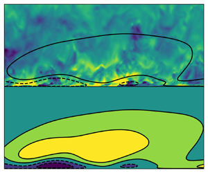
In this paper it is shown that a modal detuned instability of periodic near-wall streaks originates a large-scale structure in the bulk of the turbulent channel flow. The effect of incoherent turbulent fluctuations is included in the linear operator by means of an eddy viscosity. The base flow is an array of periodic two-dimensional streaks, extracted from numerical simulations in small domains, superposed to the turbulent mean profile. The stability problem for a large number of periodic units is efficiently solved using the block-circulant matrix method proposed by Schmid et al. (Phys. Rev. Fluids, vol. 2, 2017, 113902). For friction Reynolds numbers equal or higher than $590$, it is shown that an unstable branch is present in the eigenspectra. The most unstable eigenmodes display large-scale modulations whose characteristic wavelengths are compatible with the large-scale end of the premultiplied velocity fluctuation spectra reported in previous computational studies. The wall-normal location of the large-wavelength near-wall peak in the spanwise spectrum of the eigenmode exhibits a power-law dependence on the friction Reynolds number, similarly to that found in experiments of pipes and boundary layers. Lastly, the shape of the eigenmode in the streamwise-wall-normal plane is reminiscent of the superstructures reported in the recent experiments of Deshpande et al. (J. Fluid Mech., vol. 969, 2023, A10). Therefore, there is evidence that such large-wavelength instabilities generate large-scale motions in wall-bounded turbulent flows.

Type
JFM Papers
Copyright
© The Author(s), 2024. Published by Cambridge University Press

1. Introduction

Since the beginning of the 20th century, pattern and coherent structure formation were studied in fluid dynamics (Lord Rayleigh Reference Lord Rayleigh1916; Kraichnan & Chen Reference Kraichnan and Chen1989; Tuckerman, Chantry & Barkley Reference Tuckerman, Chantry and Barkley2020). The first evidence of such structures in wall-bounded turbulent flows dates back to Kline et al. (Reference Kline, Reynolds, Schraub and Runstadler1967), who found elongated velocity defects, called streaks, in the near-wall region of the boundary layer. The dynamics of such near-wall structures was studied by Jiménez & Moin (Reference Jiménez and Moin1991) employing numerical simulations. They showed that small computational domains, referred to as minimal flow units, were sufficient to observe self-sustained turbulence near the wall. Moreover, the minimal flow unit concept was useful to isolate the near-wall dynamics, leading to the development of the self-sustaining wall cycle theory (Hall & Smith Reference Hall and Smith1991; Hamilton, Kim & Waleffe Reference Hamilton, Kim and Waleffe1995). The cycle comprises a first phase during which streaks are amplified through the lift-up effect induced by streamwise vortices, a second phase during which streaks saturate and become unstable and a third phase that leads to the regeneration of streamwise vortices by nonlinear interactions, thus closing the cycle (Waleffe Reference Waleffe1997). Butler & Farrell (Reference Butler and Farrell1993) supported the role of the lift-up effect in the cycle with a linear transient growth computation on the turbulent channel mean profile. In addition, Jiménez & Pinelli (Reference Jiménez and Pinelli1999) showed that when near-wall streaks are artificially damped in the wall region, turbulence can not be sustained in the minimal flow unit. Therefore, the near-wall self-sustaining dynamics of turbulence in minimal flow units revolves around streaks and is well established.

Nevertheless, when larger domains and high Reynolds numbers are considered, the picture of wall turbulence becomes much more complex (Smits, McKeon & Marusic Reference Smits, McKeon and Marusic2011). Kim & Adrian (Reference Kim and Adrian1999) performed experiments on the turbulent pipe flow and reported the presence of structures having streamwise length between 12 and 14 times the pipe radius. The taxonomy of such structures in the pipe was improved by the work of Guala, Hommema & Adrian (Reference Guala, Hommema and Adrian2006), who made a distinction between very-large-scale motions (VLSMs), having a streamwise size between 8 and 16 pipe radii, and large-scale motions (LSMs), having a streamwise length of 2-3 pipe radii. Balakumar & Adrian (Reference Balakumar and Adrian2007) extended these results to turbulent channels and zero-pressure-gradient boundary layers. In these flows, the length of the large structures scales, respectively, with the channel half-height and with the boundary layer thickness. It must be noted that these experimental flows had a friction Reynolds number between $500$ and $2500$, approximately the same range investigated in this work. Furthermore, Balakumar & Adrian (Reference Balakumar and Adrian2007) observed that boundary layer flows typically have shorter VLSMs with respect to channels and pipes, a remark also made in Monty et al. (Reference Monty, Stewart, Williams and Chong2007).

Simultaneously, the experimental work of Hutchins & Marusic (Reference Hutchins and Marusic2007a) on turbulent boundary layers showed that, at a large enough friction Reynolds number ($\gtrsim$5000), there are two well-separated peaks in the premultiplied streamwise fluctuation spectrum. In general, structures having a characteristic streamwise size of $O(h)$ are referred to as LSMs and are associated with the region of the spectrum between the inner and outer peak, whereas motions having a characteristic streamwise size of $O(10h)$ are those associated with the outer peak and are referred to as VLSMs or superstructures (Hutchins & Marusic Reference Hutchins and Marusic2007a; Deshpande, de Silva & Marusic Reference Deshpande, de Silva and Marusic2023). The double peaked spectrum was observed only recently in numerical simulations of a turbulent channel (Lee & Moser Reference Lee and Moser2015; Hoyas et al. Reference Hoyas, Oberlack, Alcántara-Ávila, Kraheberger and Laux2022), due to the high computational cost of direct numerical simulations (DNS) at such high Reynolds numbers.

Investigations on LSMs and VLSMs are becoming increasingly relevant for the dynamics of wall-bounded turbulent flows. These structures carry a large fraction of the turbulent kinetic energy and of the turbulent shear stress (Guala et al. Reference Guala, Hommema and Adrian2006; Balakumar & Adrian Reference Balakumar and Adrian2007). Moreover, it has been realized recently that their control may be important for effective drag reduction in these flows (Marusic et al. Reference Marusic, Chandran, Rouhi, Fu, Wine, Holloway, Chung and Smits2021).

Large-scale motions extend to the wall and influence the near-wall region. Abe, Kawamura & Choi (Reference Abe, Kawamura and Choi2004) reported that LSMs contribute to the turbulent shear stress near the wall. Likewise, Hutchins & Marusic (Reference Hutchins and Marusic2007a) reported the existence of a footprint of the large-scale structure near the wall. However, it must be noted that this superposition effect is different from the amplitude modulation of near-wall fluctuations reported by Hutchins & Marusic (Reference Hutchins and Marusic2007b) and Mathis, Hutchins & Marusic (Reference Mathis, Hutchins and Marusic2009), which is the result of nonlinear interactions (Andreolli et al. Reference Andreolli, Gatti, Vinuesa, Örlü and Schlatter2023).

Concerning the influence of viscous effects on large-scale structures, experiments in zero-pressure-gradient boundary layers (Vincenti et al. Reference Vincenti, Klewicki, Morrill-Winter, White and Wosnik2013) and turbulent pipes (Vallikivi, Ganapathisubramani & Smits Reference Vallikivi, Ganapathisubramani and Smits2015) showed that the wall-normal location of the peak at large wavelengths of the premultiplied streamwise fluctuation spectrum scales with the square root of the friction Reynolds number. As argued by Hwang (Reference Hwang2016), this means that viscous effects are non-negligible even at large wavelengths.

The origin of large-scale structures is still uncertain. Kim & Adrian (Reference Kim and Adrian1999), Adrian, Meinhart & Tomkins (Reference Adrian, Meinhart and Tomkins2000) and Adrian (Reference Adrian2007) advanced the hypothesis that such structures may be the result of concatenation of smaller structures, which they identified with hairpin vortices. The concatenation hypothesis has been further underpinned by Lee & Sung (Reference Lee and Sung2011) and Dennis & Nickels (Reference Dennis and Nickels2011) in boundary layers and by Baltzer, Adrian & Wu (Reference Baltzer, Adrian and Wu2013) in turbulent pipes. Furthermore, Toh & Itano (Reference Toh and Itano2005) conjectured a co-supporting cycle where large-scale structures are continuously generated by small-scale near-wall structures.

On the other hand, this hypothesis has been challenged by the work of Hwang & Cossu (Reference Hwang and Cossu2010), who showed that large-scale structures can self-sustain even when smaller scales are artificially damped. Following this study, it has been proposed that a hierarchy of self-sustaining processes exists at all scales (Hwang & Cossu Reference Hwang and Cossu2011; Cossu & Hwang Reference Cossu and Hwang2017), each resembling the near-wall cycle of Hamilton et al. (Reference Hamilton, Kim and Waleffe1995).

Therefore, in this view, LSMs and VLSMs are generated by some large-scale instability and/or through a mechanism of transient growth on the mean shear (e.g. lift-up) as computed by Del Alamo & Jimenez (Reference Del Alamo and Jimenez2006) and Pujals et al. (Reference Pujals, García-Villalba, Cossu and Depardon2009) in the channel and Cossu, Pujals & Depardon (Reference Cossu, Pujals and Depardon2009) in the boundary layer. This hypothesis is further supported by the work on the resolvent analysis of McKeon & Sharma (Reference McKeon and Sharma2010) and Moarref et al. (Reference Moarref, Sharma, Tropp and McKeon2013). Whereas, secondary instabilities of the large-scale structures are advocated for the transfer of energy towards smaller scales (Park, Hwang & Cossu Reference Park, Hwang and Cossu2011; Alizard Reference Alizard2015).

The existence of a bottom-up mechanism that from near-wall structures brings to LSMs has been questioned also by Mizuno & Jiménez (Reference Mizuno and Jiménez2013), who showed that LSMs exist even without a wall, and Zhou, Xu & Jiménez (Reference Zhou, Xu and Jiménez2022), who showed that the merging of near-wall streaks is weakly correlated with LSMs.

Still, the question is not settled because there is growing statistical evidence for the concatenation hypothesis (Lee, Sung & Adrian Reference Lee, Sung and Adrian2019; Deshpande et al. Reference Deshpande, de Silva and Marusic2023). Interestingly, Doohan, Willis & Hwang (Reference Doohan, Willis and Hwang2021) showed, using a shear stress-driven two-scale model, that energy can be transferred from small scales to large scales and that this transfer corresponds to the streaks instability stage. In the present study it will be shown, by means of a modal stability analysis, that a detuned instability of periodic near-wall streaks can originate large-scale structures in the bulk of the flow.

However, the application of linear stability analyses to turbulent flows is not trivial. As discussed in the recent paper of Cossu (Reference Cossu2022), two different approaches are proposed in the literature. In the first, the equations are linearized around the base flow (often identified with the mean flow) without including a turbulence model in the linear operator (Malkus Reference Malkus1956; Butler & Farrell Reference Butler and Farrell1993; McKeon & Sharma Reference McKeon and Sharma2010). In these studies the effect of turbulent fluctuations is either neglected or included in an unknown forcing term that provides the input for a resolvent analysis (McKeon Reference McKeon2017). In the second approach, a turbulence model is included in the linear operator, often in the form of an eddy viscosity. This approach is based on the work of Reynolds & Hussain (Reference Reynolds and Hussain1972) and has been employed by Del Alamo & Jimenez (Reference Del Alamo and Jimenez2006), Cossu et al. (Reference Cossu, Pujals and Depardon2009), Pujals et al. (Reference Pujals, García-Villalba, Cossu and Depardon2009), Park et al. (Reference Park, Hwang and Cossu2011), Alizard (Reference Alizard2015), Hwang (Reference Hwang2016) and many others. There is recent evidence of the need for modelling the Reynolds stresses in linear analyses (Morra et al. Reference Morra, Semeraro, Henningson and Cossu2019). In the case of resolvent analyses on asymptotically stable mean flows, the model can be included in the forcing (Nogueira et al. Reference Nogueira, Morra, Martini, Cavalieri and Henningson2021). Whereas, as argued by Cossu (Reference Cossu2022), for modal stability analyses the model must be included in the linear operator. Therefore, this is the approach followed in this work. Cossu (Reference Cossu2022) showed that this method produces results consistent with DNS.

The rest of the paper is organized as follows. In § 2 the stability problem formulation and the numerical methods employed are outlined. In § 3 the resulting eigenspectra and leading eigenmodes are presented after a brief discussion on the considered base flow. Finally, conclusions are drawn in § 4.

2. Formulation and numerical methods

The objective of this work is to study the stability of turbulent near-wall streaks and its connection to the appearance of large-scale structures in the flow. To this aim, DNS of turbulent channel flow are performed at different Reynolds numbers (see table 1) using the channelflow code by Gibson et al. (Reference Gibson2021). Periodic boundary conditions are imposed in the streamwise and spanwise directions and no-slip conditions are used at the walls ( $y=0$ and $y=2$). The flow field is discretized by Fourier and Chebyshev collocation methods in a domain having dimensions $[L_x,L_y,L_z]$.

Table 1. Parameters of the DNS. Here $Re_b$ and $Re_{\tau }$ are the Reynolds number based respectively on the bulk velocity and the friction velocity (the channel is forced with constant bulk); $L_x/h$ and $L_z/h$ are the domain dimension respectively in the streamwise and spanwise direction scaled with the channel half-height; $N_x$ and $N_z$ are the number of Fourier modes in the streamwise and spanwise direction including dealiasing; $N_y$ is the number of Chebyshev collocation points in the wall-normal direction; $\Delta x^+$ and $\Delta z^+$ are the grid spacings in wall units in the streamwise and spanwise direction; $\Delta y^+_w$ and $\Delta y^+_c$ are the wall-normal spacings respectively near the wall and at the channel centre.

Flow variables can be either non-dimensionalized with respect to the channel half-height $h$ and mean bulk velocity $U_b=1/\varOmega \int _{\varOmega } u\,{\rm d}\varOmega$ or with respect to the friction velocity $u_{\tau }=\sqrt {\tau _w/\rho }$ and the viscous length scale $\delta _{\nu }=\nu /u_{\tau }$, $\nu$ being the kinematic viscosity. These quantities define the turbulent Reynolds number $Re_\tau =u_{\tau } h /\nu$. Variables expressed in the latter (inner) units are referred to with the superscript $^+$, whereas, from now on, variables without any superscript are scaled in the former (outer) units.

The size of the computational domains, the number of Fourier modes and Chebyshev collocation points and the grid spacings in wall units are listed in table 1. Note that the flow cases without any subscript are those used for the base flow computation, which considers rather small (although larger than the minimal flow units) domains. For instance, for $Re_{\tau}\approx 1000$, we have used a minimal box for the logarithmic layer as in Jiménez (Reference Jiménez2013), which is known to have incorrect statistics above $y \approx L_z/3 \approx 0.25h$ (Flores & Jiménez Reference Flores and Jiménez2010; Lozano-Durán & Jiménez Reference Lozano-Durán and Jiménez2014). However, it must be observed that the only purpose of these simulations is to extract the near-wall coherent structures used for the stability analysis, which, using spanwise-periodic conditions, allows the computation of coherent structures of much longer wavelengths than those of the base flow. Whereas, the flow case indicated in table 1 with the subscript $L$ has been run with a computational domain sufficiently large for allowing the development of large-scale structures, and will be used for validation of the wavelengths and eigenmodes found by the stability analysis. The validity of our DNS data for this purpose is further discussed in Appendix A.

The base flow for the stability analysis is composed of the long-time averaged flow plus near-wall streaky coherent structures. The mean flow profile is obtained using a semi-analytical model (Reynolds & Tiederman Reference Reynolds and Tiederman1967), whereas the near-wall streaks are extracted from DNS data by means of proper orthogonal decomposition (POD). It has been shown in previous studies (Moin & Moser Reference Moin and Moser1989; Alfonsi & Primavera Reference Alfonsi and Primavera2007) that the leading POD mode for the turbulent channel flow is constituted by streamwise uniform streaks. However, in the near-wall region of turbulent flows, as indicated by the early works of Hamilton et al. (Reference Hamilton, Kim and Waleffe1995) and more recently discussed in Jiménez (Reference Jiménez2022), due to the establishment of the wall cycle, velocity streaks exhibit small inclinations with respect to the streamwise direction due to the sinuous/varicose modulations induced by their secondary instability. This can be visualized in figure 1, which provides a snapshot of the DNS velocity field after filtering out the flow structures with spanwise wavelengths $\lambda _z^+<80$ and $\lambda _z^+>220$. The dashed lines, having angle $\theta =14^{\circ }$ with respect to the streamwise direction, show a mild inclination of the coherent structures in the wall region. Qualitatively similar structures are found in the larger domain DNS at $Re_{\tau }=1000$ (not shown). However, it must be noted that these streaks are inclined with different angles. Whereas, we will consider a more idealized situation where the streaks are periodic along a given direction, i.e. they are all inclined with the same angle. This is a necessary approximation in order to apply the block-circulant matrix method described below.

Figure 1. Direct numerical simulation snapshots of the streamwise velocity fluctuation at (a) $Re_{\tau }=590$ and (b) $Re_{\tau }=1000$ in a wall-parallel plane at $y^+ \approx 40$. The velocity field is filtered in the spanwise direction with wavelengths $80<\lambda _z^+<220$. The dashed lines, having angle $\theta =14^{\circ }$ with respect to the streamwise direction, show the mild inclination of the coherent structures in the wall region. These inclined streaky structures are extracted by POD for analysing their secondary instability.

For this reason, we extract by POD arbitrarily inclined coherent structures considering the Fourier decomposition of the instantaneous flow field $\boldsymbol {u}$ in the streamwise ($x$) and spanwise ($z$) directions (Muralidhar et al. Reference Muralidhar, Podvin, Mathelin and Fraigneau2019):

(2.1)\begin{equation} \boldsymbol{u}(\boldsymbol{x}, t) = \sum_{k_x,k_z} \hat{\boldsymbol{u}}_{k_x,k_z}(y,t) \,{\rm e}^{2{\rm \pi} {\rm i} ( {k_x x}/{L_x} + {k_z z}/{L_z})} . \end{equation}

Here ${\rm i}$ denotes the imaginary unit and the sum is extended to all the Fourier modes used for the discretization of the domain, while $y$ denotes the wall-normal direction. For a given wavenumber couple $\{k_x, k_z\}$, POD is performed using the profiles $\hat {\boldsymbol {u}}_{k_x,k_z}(y,t)$ obtained from $2000$ three-dimensional snapshots of the small-domain DNS, equi-spaced in time with non-dimensional time step $\Delta t U_b/h= 0.25$. Convergence of the POD was assessed by repeating the computation with $1200$ snapshots. The resulting POD eigenvalues and eigenvectors showed minor differences with respect to the case with $2000$ snapshots, as did the corresponding stability analysis results. Therefore, it can be concluded that the chosen number of snapshots for the POD does not qualitatively affect the outcome of the stability analysis. In one case, the POD has been repeated with $4000$ snapshots, in order to address an issue described below (see discussion in § 3.1).

The leading POD profile obtained, $\hat {\boldsymbol {\psi }}_{k_x,k_z}(y)$, is used to reconstruct a three-dimensional flow field as

(2.2)\begin{equation} \boldsymbol{u}_s(\boldsymbol{x})=\hat{\boldsymbol{\psi}}_{k_x,k_z}(y)\,{\rm e}^{2{\rm \pi} {\rm i} ({k_x x}/{L_x} + {k_z z}/{L_z})} + \text{ c.c.}, \end{equation}

where c.c. denotes complex conjugate. The properties of the POD (Berkooz, Holmes & Lumley Reference Berkooz, Holmes and Lumley1993) ensure that the mode obtained in this way is still a POD mode for the three-dimensional channel. In addition, using this method, the inclination of the resulting coherent structures can be freely chosen selecting $k_x$ and $k_z$. Note that, being selected a priori, this inclination is not expected to vanish as the number of snapshots used for the POD is increased. Note that, for a given couple $\{k_x, k_z\}$, there is a paired $\{k_x, -k_z\}$ mode that provides streaks inclined with the same angle in the opposite direction. However, in order to obtain a two-dimensional base flow (see below), the two modes can not be employed together. It is a limitation of the current approach to consider only two-dimensional base flows.

The extracted structures are uniform along the direction $\bar {x}$, which is inclined with respect to $x$ of an angle $\theta =\arctan [ ( k_xL_z) / ( k_zL_x) ]$. In order to make the stability analysis computationally cheaper, we exploit this spatial homogeneity by rotating the POD mode in the $y$$\bar {z}$ plane, where $\bar {z}$ is the axis perpendicular to $\bar {x}$. The base flow is thus constructed adding the mean turbulent flow to the rotated streaky POD mode $\overline {\boldsymbol {u}_s}$. Because the POD modes are defined up to an arbitrary multiplicative constant, we introduce an amplitude definition as in Alizard (Reference Alizard2015):

(2.3)\begin{equation} A = \frac{\max_{y,\bar{z}} u - \min_{y,\bar{z}} u}{2U_{c}}. \end{equation}

Here $u$ (scalar) is the streamwise component of a two-dimensional velocity field and $U_{c}$ is the centreline velocity of the mean turbulent profile.

Before adding the streaky mode to the mean flow, the amplitude of the POD mode is normalized such that the streaks have a chosen amplitude $A_s$. More explicitly, let $\overline {\boldsymbol {u}_s}$ be the streaky mode in the rotated frame with an arbitrary amplitude (i.e. before normalization), the normalized mode $\overline {\boldsymbol {u}_s}^{A_s}$ is given by

(2.4)\begin{equation} \overline{\boldsymbol{u}_s}^{A_s} = \frac{A_s}{\dfrac{\max_{y,\bar{z}} \overline{u_s} - \min_{y,\bar{z}} \overline{u_s}}{2U_{c}}} \overline{\boldsymbol{u}_s}. \end{equation}

Note that $A_s$ is a free parameter of the problem, whose choice will be made on the basis of DNS data, as discussed in the next section. The base flow is thus constructed as

(2.5)\begin{equation} \boldsymbol{U}(y,\bar{z})=\langle \boldsymbol{u} \rangle (y)+ \overline{\boldsymbol{u}_s}^{A_s}(y,\bar{z}) , \end{equation}

where $\langle {\cdot } \rangle$ denotes the averaging in time and in the wall-parallel spatial directions.

The instability of this $\bar {z}$-modulated base flow is thus addressed linearizing the Navier–Stokes equations around this two-dimensional base flow as (Park et al. Reference Park, Hwang and Cossu2011; Alizard Reference Alizard2015)

(2.6)\begin{equation} \left.\begin{gathered} \frac{\partial{u_i^\prime}}{\partial{t}} ={-}U_j \frac{\partial{u_i^\prime}}{\partial{\bar{x}_j}} -u^\prime_j \frac{\partial{U_i}}{\partial{\bar{x}_j}} - \frac{\partial{p^\prime}}{\partial{\bar{x}_i}} + \frac{\partial}{\partial \bar{x}_j}\left[ ( \nu + \nu_t)\left( \frac{\partial{u^\prime_i}}{\partial{\bar{x}_j}} + \frac{\partial{u^\prime_j}}{\partial{\bar{x}_i}}\right) \right],\\ \frac{\partial{u^\prime_i}}{\partial{\bar{x}_i}}=0, \end{gathered}\right\} \end{equation}

where $\nu =1/Re_b$ is the non-dimensional viscosity and $^\prime$ denotes the perturbations. A detailed derivation is provided in Appendix B. Despite the perturbation verifying the linear equations (2.6), the base flow does not verify the corresponding steady nonlinear equations as would be the case in classical hydrodynamic stability analyses. This work relies on a frozen base flow assumption, which is common to numerous previous studies on the secondary instability of streaks (Schoppa & Hussain Reference Schoppa and Hussain2002; Marquillie, Ehrenstein & Laval Reference Marquillie, Ehrenstein and Laval2011; Park et al. Reference Park, Hwang and Cossu2011; Hack & Zaki Reference Hack and Zaki2014; Alizard Reference Alizard2015; Hack & Moin Reference Hack and Moin2018). This working hypothesis is a weak point of the approach because it is difficult to substantiate in a turbulent flow (see § 3.1 for further details), but it is not clear at present how to relieve it.

Following Park et al. (Reference Park, Hwang and Cossu2011), Alizard (Reference Alizard2015) and also the recent work of Cossu (Reference Cossu2022), the effect of the turbulent fluctuations in the stability problem is taken into account using the eddy viscosity model proposed by Cess (Reference Cess1958), i.e.

(2.7)\begin{align} \nu_t = \frac{1}{2Re_b}\left \{ \left[ 1 + \left( \frac{Re_{\tau}k}{3} ( 2y-y^2) ( 3-4y+2y^2) \left( 1-\frac{Re_{\tau}}{A}\,{\rm e}^{\lvert y-1 \rvert-1}\right) \right)^2 \right]^{1/2} - 1 \right\}, \end{align}

with $k=0.426$, $A=25.4$ (Del Alamo & Jimenez Reference Del Alamo and Jimenez2006) and $y \in [0,2]$. Computing the eddy viscosity from the minimal DNS data after subtraction of the projected POD mode (following Tammisola & Juniper Reference Tammisola and Juniper2016) gave minor differences with respect to the Cess (Reference Cess1958) model, which did not qualitatively affect the results of the paper. This being the case, the Cess (Reference Cess1958) formula is preferred because it avoids the singularity at the channel centre in the definition of the eddy viscosity (where the mean flow gradient tends to zero).

Then, a normal mode ansatz with complex frequency $\sigma$ and real streamwise wavenumber $\alpha$, namely,

(2.8)\begin{equation} \boldsymbol{q}^\prime(\bar{x},y,\bar{z},t) = {\rm e}^{\sigma_r t} \tilde{\boldsymbol{q}}(y,\bar{z}) \,{\rm e}^{{\rm i} (\alpha \bar{x} + \sigma_i t)} + \text{ c.c. } \end{equation}

is injected in the linearized Navier–Stokes equations for the secondary perturbation $\boldsymbol {q}^\prime =(\boldsymbol {u}^\prime,p^\prime )^\textrm {T}$ and the following generalized eigenvalue problem is obtained:

(2.9)\begin{equation} \sigma {{\boldsymbol{\mathsf{B}}}}\,\tilde{\boldsymbol{q}} = {{\boldsymbol{\mathsf{A}}}}\,\tilde{\boldsymbol{q}}. \end{equation}

Here

(2.10) $$\begin{gather} {{\boldsymbol{\mathsf{B}}}} =\begin{bmatrix} 1 & 0 & 0 & 0 \\ 0 & 1 & 0 & 0 \\ 0 & 0 & 1 & 0 \\ 0 & 0 & 0 & 0 \end{bmatrix},\quad {{\boldsymbol{\mathsf{A}}}} = \begin{bmatrix} \mathscr{L} & -U_y + {\rm i}\alpha\nu_t' & -U_{\bar{z}} & -{\rm i}\alpha \\ 0 & \mathscr{L} - V_y + \nu_t' D_y & -V_{\bar{z}} & -D_y \\ 0 & -W_y + \nu_t' D_{\bar{z}} & \mathscr{L} - W_{\bar{z}} & -D_{\bar{z}} \\ {\rm i}\alpha & D_y & D_{\bar{z}} & 0 \end{bmatrix}, \end{gather}$$
(2.11)$$\begin{gather}\mathscr{L} ={-}{\rm i}\alpha U -V D_y -W D_{\bar{z}} + ( \nu + \nu_t) \nabla^2 + \nu_t' D_y, \end{gather}$$

where $D_{y,\bar {z}}$ denotes differentiation with respect to $y$ or $\bar {z}$, $\nabla ^2 =-\alpha ^2 + D_y^2 + D_{\bar {z}}^2$ is the Laplacian operator, $U_{y,\bar {z}},V_{y,\bar {z}},W_{y,\bar {z}}$ are the base flow components differentiated with respect to $y$ or $\bar {z}$ and $\nu _t'$ is the eddy viscosity differentiated with respect to $y$.

Now, note that the considered two-dimensional base flow is periodic by construction in the $\bar {z}$ direction. Then, the instability of an array of periodic streaks can be studied efficiently using the block-circulant matrix formalism proposed by Schmid, De Pando & Peake (Reference Schmid, De Pando and Peake2017). Using this method, the computation of the stability of a system composed by $N_u$ repeated subunits is reduced to $N_u$ subunit-size computations, each associated to a root of unity $\rho _j = \exp ( 2{\rm \pi} \textrm {i}\, j/N_u)$ with $j=0,1,\ldots,N_u-1$. Here, a subunit is a two-dimensional $y-\bar {z}$ domain periodic in $\bar {z}$.

The first step consists in reordering the system as a partition in $N_u$ subsystems corresponding to the $N_u$ subunits. Thus, the eigenvalue problem is recast as

(2.12)\begin{align} \sigma \underbrace{\begin{pmatrix} {{\boldsymbol{\mathsf{B}}}} & \unicode{x22EF} & \unicode{x22EF} \\ \unicode{x22EF} & {{\boldsymbol{\mathsf{B}}}} & \unicode{x22EF} \\ \vdots & \vdots & \vdots \\ \unicode{x22EF} & \unicode{x22EF} & {{\boldsymbol{\mathsf{B}}}} \end{pmatrix} }_{{{\boldsymbol{\mathsf{B'}}}}} \underbrace{\begin{pmatrix} \tilde{\boldsymbol{q}}^{(0)} \\ \tilde{\boldsymbol{q}}^{(1)} \\ \vdots \\ \tilde{\boldsymbol{q}}^{(N_u-1)} \end{pmatrix}}_{\tilde{\boldsymbol{q}}} =\underbrace{\begin{pmatrix} {{\boldsymbol{\mathsf{A}}}}^{(0)} & {{\boldsymbol{\mathsf{A}}}}^{(1)} & \unicode{x22EF} & {{\boldsymbol{\mathsf{A}}}}^{(N_u-1)} \\ {{\boldsymbol{\mathsf{A}}}}^{(N_u-1)} & {{\boldsymbol{\mathsf{A}}}}^{(0)} & \unicode{x22EF} & {{\boldsymbol{\mathsf{A}}}}^{(N_u-2)} \\ \vdots & \vdots & & \vdots \\ {{\boldsymbol{\mathsf{A}}}}^{(1)} & {{\boldsymbol{\mathsf{A}}}}^{(2)} & \unicode{x22EF} & {{\boldsymbol{\mathsf{A}}}}^{(0)} \end{pmatrix}}_{{{\boldsymbol{\mathsf{A'}}}}} \underbrace{\begin{pmatrix} \tilde{\boldsymbol{q}}^{(0)} \\ \tilde{\boldsymbol{q}}^{(1)} \\ \vdots \\ \tilde{\boldsymbol{q}}^{(N_u-1)} \end{pmatrix}}_{\tilde{\boldsymbol{q}}}, \end{align}

where ${{\boldsymbol{\mathsf{A'}}}}$ is the Jacobian associated to the stability problem composed of the matrices ${{\boldsymbol{\mathsf{A}}}}^{(j)}$ (for $j=0,\ldots,N_u-1)$ describing the dynamics in a subunit and the interactions between subunits, and the disturbance in the $j$th subunit is denoted as $\tilde {\boldsymbol {q}}^{(j)}$. The Jacobian matrix ${{\boldsymbol{\mathsf{A'}}}}$ is block circulant due to the specific $N_u$-periodic nature of the system and becomes a block-diagonal matrix $\hat {{{\boldsymbol{\mathsf{A}}}}}$ using the similarity transformation

(2.13)\begin{equation} {{\boldsymbol{\mathsf{P}}}}^H {{\boldsymbol{\mathsf{A'}}}} {{\boldsymbol{\mathsf{P}}}} = \text{diag}(\hat{{{\boldsymbol{\mathsf{A}}}}}^{(0)}, \hat{{{\boldsymbol{\mathsf{A}}}}}^{(1)},\ldots, \hat{{{\boldsymbol{\mathsf{A}}}}}^{(N_u-1)} ) \equiv \hat{{{\boldsymbol{\mathsf{A}}}}}, \end{equation}

where the transfer matrix ${{\boldsymbol{\mathsf{P}}}}$ is defined as

(2.14)\begin{equation} {{\boldsymbol{\mathsf{P}}}} = {{\boldsymbol{\mathsf{J}}}} \otimes {{\boldsymbol{\mathsf{I}}}}, \end{equation}

with ${{\boldsymbol{\mathsf{J}}}}$ a matrix such that ${{{J}}}_{j+1,k+1} = \rho _j^k/\sqrt {N_u}$ for $j,k={0},\ldots, N_u-1$ and $\rho _j = \exp (2\textrm {i}{\rm \pi} j/N_u)$ the $j$th of the $N_u$ roots of unity. The symbol $\otimes$ denotes the Kronecker product and ${{\boldsymbol{\mathsf{I}}}}$ the identity matrix. Using this similarity transformation, the full linear stability problem is thus reduced to that of the $N_u$ subsystems characterized by the matrices $\hat {{{\boldsymbol{\mathsf{A}}}}}^{(j)}$. From (2.13) follows that

(2.15)\begin{equation} \hat{{{\boldsymbol{\mathsf{A}}}}}^{(j)} = \sum_{k=0}^{N_u-1} \rho_j^k {{\boldsymbol{\mathsf{A}}}}^{(k)}. \end{equation}

The full eigenspectrum of the matrix ${{\boldsymbol{\mathsf{A}}}}'$ is found merging the $N_u$ spectra of $\hat {{{\boldsymbol{\mathsf{A}}}}}^{(j)}$ for $j={0},\ldots,N_u-1$. Similarly, provided $\boldsymbol {v}_j$ is an eigenvector of $\hat {{{\boldsymbol{\mathsf{A}}}}}^{(j)}$, the eigenfunctions of the full system can be retrieved and take the form $[\boldsymbol {v}_j, \rho _j \boldsymbol {v}_j, \rho _j^2 \boldsymbol {v}_j,\ldots, \rho _j^{N_u-1} \boldsymbol {v}_j]^\textrm {T}$ for $j={0},\ldots,N_u-1$.

Physically, the argument of the root of unity $\arg (\rho _j)=2{\rm \pi} j/N_u$$j=1,\ldots,N_u-1$) acts as a phase shift between the different subunits: the farther it is from $0$ (or $2{\rm \pi}$), the more desynchronised the mode is. After $2{\rm \pi} /\arg (\rho _j) = N_u/j$ subunits, the cumulative phase shift will exceed $2{\rm \pi}$, giving an estimate of the effective fundamental period of the eigenfunction of the full system. Therefore, this formalism allows the analysis of a very large size system composed of small subunits such as near-wall streaks, possibly prone to large-scale instabilities (Jouin et al. Reference Jouin, Ciola, Cherubini and Robinet2024).

For each subunit, the stability problem (2.9) is discretized with $N_z=60$ Fourier modes in the $\bar {z}$ direction and $N_y=129$ Chebyshev modes in the wall-normal direction. Some computations have been repeated increasing the resolution to $N_z \times N_y = 100 \times 201$, showing minor changes both on the eigenvalues (variation smaller than $2\,\%$ with respect to the previous resolution) and on the shape of the eigenvectors. This validation has been carried out at the largest Reynolds number considered, which, in principle, would require the finest discretization. Hence, the coarser previously mentioned discretization is deemed appropriate and used for all the other computations.

3. Results

3.1. Base flow

An example of the wall-close coherent structures extracted using POD is shown in figure 2(a). The two-dimensional base flow constructed adding these structures with amplitude $A_s=0.25$ to the mean flow is shown in figure 2(b). As can be remarked from the arrows on this panel, the streamwise velocity modulations are subject to a non-zero mean flow component in the $\bar {z}$ direction, due to their inclination with respect to the streamwise direction.

Figure 2. Base flow for the $Re_{\tau } = 590$ case. (a) Isocontours of the streamwise component of the POD mode with $k_x=1$ and $k_z=2$ ($\theta \approx 14^{\circ }$). (b) Base flow (POD mode plus mean flow) visualized in the $y$$\bar {z}$ plane: isocontours of the streamwise component and arrows for the tranverse components.

It can be noted that the extracted streaks are not symmetric with respect to the channel mid-plane. For this reason, we repeated the POD for $Re_{\tau }=590$, $k_x=1$ and $k_z=2$ with $4000$ snapshots instead of $2000$. Comparing panel (a) with panel (c) in figure 3 it can be observed that the asymmetry persists. Moreover, it has been remarked that the first two POD modes have comparable eigenvalues and seem to be always in phase opposition (compare panel (a) with panel (b) and panel (c) with panel (d)). Hence, the first two POD modes are indeed coupled. A linear combination of these two modes would be arbitrary because their amplitudes are not defined (we define only a relative amplitude of the streaks with respect to the mean flow, as described above). Therefore, the asymmetric mode was retained.

Figure 3. Root mean square of the POD streaky modes for $Re_{\tau }=590$, $k_x=1$, $k_z=2$ (the mean is computed along $x$ and $z$). The POD modes are obtained from (a,b) 2000 DNS snapshots and (c,d) 4000 DNS snapshots spaced at $\Delta t = 0.25 h/U_b$ in time. (a,c) First leading mode, (b,d) second leading mode. The dashed lines denote $y/h=0.25$ and $y/h=1.75$ and delimit the wall regions where the turbulent flow is well resolved in the minimal domains.

In figure 3 it can also be noted that the POD mode decreases rapidly when the distance from the wall is greater than $0.25h$, as demarcated by the dashed black lines. The flow in the minimal unit is well resolved in this region (Flores & Jiménez Reference Flores and Jiménez2010). For larger $k_x$ and $k_z$, the mode is even more localized near the wall. Whereas, it is dislocated towards the channel centre for $k_x=1$ and $k_z=1$. However, as shown in the following, this particular combination of wavenumbers is not much relevant for the conclusions of the paper and is included in the results only for completeness.

In order to define a realistic variability range for $A_s$, some quantitative measurements are performed on the DNS data. For each snapshot, (2.3) is applied to every $y$$z$ plane and averaged in the streamwise direction and in time. The result is an amplitude of ${\approx }0.3 \pm 0.01$ (blue crosses in figure 4) for all the four Reynolds number considered, where the uncertainty is given by the standard deviation in time. Evidently, this is a rough estimate because (2.3) is applied to an instantaneous turbulent field, which is rather different from the base flow constituted by periodic streaky structures. Using (2.3), the amplitude is computed using the maximum and minimum values of the streamwise component of velocity, irrespective of the structural topology of the velocity field, in a sort of worst case scenario. Therefore, this can be considered an upper estimate on the streaks amplitude.

Figure 4. Amplitude $A$ (2.3) measured in the DNS for different Reynolds numbers; the symbols denote the temporal mean value while the error bars denote the respective standard deviation. The circles are the peaks in the r.m.s. profiles of the streamwise fluctuation scaled with $U_c$ (see also figure 14b).

On the other hand, the root-mean-square (r.m.s.) peak value of the streamwise velocity fluctuation (scaled with the centreline velocity for comparison) is around $0.1$, as shown by the black circles in figure 4. Given the definition of r.m.s., it is sure that a greater value will be attained by the velocity fluctuation at least at some instant of time. Thus, it is argued that a realistic amplitude for the coherent structures must fall in the range $0.1\div 0.3$. This estimation from the DNS is performed on the full velocity fluctuation, whereas the considered base streaks are made up of only one Fourier mode. The energy contained in one Fourier mode of the DNS fields is not so substantial, because of the broadband character of the turbulent velocity spectrum. Therefore, the extracted mode should not be seen as representative of the $(k_x, k_z)$ Fourier mode alone but, rather, as an idealized representative of the whole ensemble of near-wall coherent turbulent fluctuations. In practice, the coherent turbulent spectrum was condensed into one mode. This is a very strong approximation, but it is necessary in our current approach. Note, also, that the values used by Park et al. (Reference Park, Hwang and Cossu2011) and Alizard (Reference Alizard2015) are included in the same range.

Moreover, the stability equations are derived assuming that the base flow $\boldsymbol {U}$ verifies the following equation (see Appendix B):

(3.1)\begin{equation} \frac{\partial{U_i}}{\partial{t}} ={-} U_j\frac{\partial{U_i}}{\partial{\bar{x}_j}} - \frac{\partial{P}}{\partial{\bar{x}_i}} + \frac{\partial{}}{\partial{\bar{x}_j}}\left[ ( \nu+\nu_t)\left( \frac{\partial{U_i}}{\partial{\bar{x}_j}}+\frac{\partial{U_j}}{\partial{\bar{x}_i}}\right) \right]. \end{equation}

If the right-hand side is zero then the base flow is steady and one can legitimately fomulate the stability problem as an eigenvalue problem. If $\boldsymbol {U}$ is unsteady but periodic in time, one can use Floquet theory and still define eigenvalues and eigenmodes. In the case considered here, $\boldsymbol {U}$ is neither steady nor periodic but has a general time dependence dictated by (3.1). In these cases, one usually employs the frozen base flow assumption which means that $\boldsymbol {U}$ is treated as if it were steady. This implies that the right-hand side of (3.1) is somewhat neglected in the stability equations. Therefore, the assumption can be tested by comparing the time derivative of $\boldsymbol {u}^\prime$ with the time derivative of $\boldsymbol {U}$. It must be taken into account that $\boldsymbol {u}^\prime$ is defined up to a multiplicative constant. Therefore, we consider

(3.2a,b)\begin{equation} \frac{1}{\lVert \boldsymbol{u}^\prime \rVert}\left\lVert \frac{\partial{\boldsymbol{u}^\prime}}{\partial{t}} \right\rVert \approx \lvert \sigma \rvert \quad \text{and} \quad \varSigma := \frac{1}{\lVert \boldsymbol{U}^\prime \rVert}\left\lVert \frac{\partial{\boldsymbol{U}^\prime}}{\partial{t}} \right\rVert, \end{equation}

where $\sigma$ is the complex frequency of the mode and $\lVert {\cdot } \rVert$ is the $L^2$ norm on the $y$$\bar {z}$ domain. Then, the frozen base flow assumption is justified if the ratio $\varSigma /\lvert \sigma \rvert$ is small. This ratio has been computed for several of the parameter combinations explored in the following sections and has been found in most cases smaller than $1$. Only in few cases, however, it is smaller than $0.1$, confirming that the frozen base flow assumption is only partially corroborated. This is a limitation of the current study.

3.2. Leading growth rates

Examples of eigenspectra are given in figure 5 for two of the four friction Reynolds numbers considered in this study, $Re_\tau =180$ (a) and $Re_\tau =590$ (b), for $N_u=60$ subunits. The colourbar shows the respective detuning factor ($\epsilon _j=j/N_u$) of the instability, which is allowed to take $N_u$ discrete equi-spaced values in the interval $[0,1)$. Due to the high number of subunits considered, the eigenspectra show numerous branches. Figure 5 shows that one of these branches is almost marginally stable at $Re_{\tau }=180$ and becomes prone to a detuned instability ($0.9<\epsilon _j<1$) at a higher Reynolds number. However, it must be noted that the detuning factor depends on the reference frame, so that the effective detuning factor in the streamwise-aligned ($x$$z$) reference frame is lower. Nevertheless, the actual value of the detuning factor is of minor significance for the purpose of this paper. The important message of figure 5 is that an unstable branch is present at a sufficiently high Reynolds number, with the leading mode corresponding to a detuned instability.

Figure 5. Eigenspectra for the $A_s = 0.25$ and $\alpha =1.0$ case ($N_u=60$, $\theta \approx 14^{\circ }$) at (ac) $Re_{\tau }=180$ and (bd) $Re_{\tau }=590$. The colours denote the detuning factor $\epsilon _j = j/N_u$ for $j=0,\ldots,N_u-1$. The top row panels are close-ups on the portion of the spectrum denoted by solid line rectangles in the bottom row panels. The dashed black line denotes the marginal stability limit ($\sigma _r=0$). The point with maximum growth rate $\sigma _r$ defines the leading unstable mode in the case of instability ($\max \sigma _r>0$) or the least stable mode in the case of stability ($\max \sigma _r<0$).

We verified that the number of subunits has a weak impact both on the eigenspectra and on the eigenmodes, provided that it is sufficiently large (e.g. $N_u\ge 60$, see details in Appendix D). This behaviour is expected because the number of units fixes the maximum allowable spanwise size of the modes. If this size is too small, modes linked to a large-scale spanwise modulation might not be properly resolved. On the other hand, if the domain is sufficiently large, the leading mode is properly resolved and becomes independent of the domain size. Whereas, the streaks amplitude $A_s$ and the inclination of the base flow streaks $\theta$ strongly affect the outcome of the stability analysis, as shown in figure 6. The growth rates of the most unstable modes have similar values and trends for $Re_{\tau }=590$, $Re_{\tau }=1000$ and $Re_{\tau }=2000$ (blue, red and yellow lines), while the $Re_{\tau }=180$ (green) cases show a different behaviour.

Figure 6. Growth rate of the leading unstable mode ($\star$) or least stable mode ($\bullet$) as a function of (a) the base flow streaks amplitude (with $\alpha =1.0$ and $k_z=2$), (b) the inclination of the base flow (with $\alpha = 1.0$ and $A_s=0.20$), (c) the streamwise wavenumber $\alpha$ (with $A_s=0.20$ and $k_z=2$). All computations were performed with $k_x=1$ and $N_u=60$.

The dependence of the most unstable mode growth rate on the base flow streaks amplitude is displayed in figure 6(a). As expected, the growth rate increases linearly with this parameter so that instability is found for $A_s>0.1$ for $Re_{\tau }=590$, 1000, 2000. For $Re_{\tau }=180$, instability is found only at a very large amplitude $A_s>0.25$.

Concerning the base flow inclination, figure 6(b) shows that there is a peak in the growth rate at $\theta \approx 14^{\circ }$ for $Re_\tau =590$, 1000 slightly displaced at $\theta \approx 7.1^{\circ }$ for $Re_{\tau }=2000$, while the flow remains stable at $Re_{\tau }=180$. This decrease of the optimal angle with the friction Reynolds number might indicate a trend towards the destabilisation of more streamwise-aligned streaky structures at higher Reynolds numbers. Whereas, for $Re_{\tau }=180$ and $A_s<0.25$, the base flow remains stable no matter the angle of the POD mode. The stability of the $Re_{\tau }=180$ cases can be attributed to low-Reynolds-number effects and is compatible with the poor evidence of large-scale structures in these flow conditions (Smits et al. Reference Smits, McKeon and Marusic2011).

The wavenumber along $\bar {x}$, namely, $\alpha$, is a free parameter of the problem as well. Figure 6(c) shows that, for the intermediate Reynolds number considered ($590$, $1000$), there is a plateau in the growth rate for $\alpha \in [1.0,2.0]$. The plateau is shifted towards smaller wavenumbers ($\alpha \in [0.5,1.5]$) for $Re_{\tau }=2000$. Whereas, for $Re_{\tau }=180$, the growth rate is found positive for the streaks amplitude $A_s=0.2$ only for $\alpha =2.0$.

Hence, the influence of $\alpha$ on the growth rate gives a range of unstable wavenumbers depending on the friction Reynolds number. The fact that the most unstable wavenumber decreases when $Re_\tau$ grows is consistent with the observation of coherent structures having a larger streamwise wavelength at a higher friction Reynolds number (compare the premultiplied energy spectra at different $Re_\tau$ in figure 10 and the work of Del Alamo et al. Reference Del Alamo, Jiménez, Zandonade and Moser2004). As shown in the next section, this range of $\alpha$ gives a range of streamwise and spanwise wavelengths in the DNS reference frame.

Finally, one may ask what happens when both the base flow wavenumbers ${k_x,k_z}$ are changed. To investigate this point, several computations spanning $k_x=[0, 1, 2, 4, 8]$ and $k_z=[1, 2, 4, 8]$ for the two intermediate Reynolds numbers considered ($Re_{\tau }=[590, 1000]$) were performed having fixed $A_s=0.20$, $\alpha =1.0$ and $N_u=60$. The resulting growth rates are shown in figure 7. Two aspects can be remarked: (i) the streamwise independent ($k_x=0$) structures result is always stable; (ii) increasing $k_z$, the maximum growth rate moves towards larger $k_x$. This means that the instability is found in a given range of the ratio $k_z/k_x$ that corresponds to a range of inclination angles $\theta \approx 7^\circ \div 28^\circ$.

Figure 7. Growth rate of the leading unstable mode ($\star$) or least stable mode ($\bullet$) as a function of base flow wavenumbers $\{k_x,k_z\}$ for (a) $Re_{\tau }=590$ and (b) $Re_{\tau }=1000$. All computations were performed with $\alpha =1.0$, $A_s=0.20$ and $N_u=60$.

3.3. Leading eigenmodes

In this subsection some observations on the leading unstable modes (or least stable modes in some cases) are presented. The $Re_{\tau } = 180$ case, for which evidence of LSMs is not compelling, will not be considered. Moreover, we fix $k_x=1$ and $k_z=2$ for most of the section to simplify the analysis. It will be argued that other combinations of base flow wavenumbers $\{k_x,k_z\}$ lead to similar conclusions. Whereas, different $\alpha \in [0.5,2]$ will be considered unless differently specified.

A closer look to the eigenmodes spatial structure is provided in figure 8, where the energy content of the mode is represented with respect to the wavelength along $\bar {z}$ ($\bar {\lambda }_z$) and to the wall-normal position. To be more precise, consider the eigenvector $\tilde {\boldsymbol {q}}(y,\bar {z})=[\tilde {u}(y,\bar {z}),\tilde {v}(y,\bar {z}),\tilde {w}(y,\bar {z}),\tilde {p}(y,\bar {z})]^\textrm {T}$ and its Fourier transform in the $\bar {z}$ direction $\hat {\tilde {\boldsymbol {q}}}$. The quantity plotted in figure 8 is $E_{uu}(y,\bar {\lambda }_z) = \hat {\tilde {u}}\hat {\tilde {u}}^*$, where $^*$ denotes the complex conjugate. It can be seen in the figure that the eigenmodes are made up of several waves with different wavelengths. Among them, one is characterized by a large wavelength and extends up to the outer region of the flow ( $y/h>0.1$). In the figure the spanwise wavelength characterizing the base flow is denoted by the black solid line. Therefore, it is evident that the large-wavelength component of the eigenmode is much more extended than the base flow structures. We postulate that the large-wavelength modulation found in the unstable eigenmode is a large-scale structure engendered by the interaction of several base flow subunits, i.e. several near-wall streaks. In the wall-normal direction the eigenmodes have two peaks at large wavelength: one in the wall layer ( $y<0.1$) and the other in the outer layer ( $y>0.1$). The outer one is the presumed large-scale structure, while the inner one can be interpreted as the near-wall footprint of this structure, as described by Hutchins & Marusic (Reference Hutchins and Marusic2007a). The other short-wavelength modulations that are present near the wall can be attributed to the near-wall cycle (Hamilton et al. Reference Hamilton, Kim and Waleffe1995).

Figure 8. Spectral energy content along the $\bar {z}$ direction of the streamwise component of the leading unstable eigenmodes ($E_{uu}$ in the text) for $\alpha =1.0$ and different Reynolds numbers ($A_s=0.20$, $k_x=1$, $k_z=2$). The vertical black line denotes the wavelength of the subunits (the base flow is periodic along $\bar {z}$ with this wavelength). The eigenmode is normalized to have kinetic energy equal to one. The contour levels are for $E_{uu}=[10^{-4}, 10^{-1}]$. The two different background colours indicate the inner layer (light grey for $y<0.1$) and the bulk of the flow (light blue for $y>0.1$).

It is interesting to investigate how the wall-normal position of the inner peak at large wavelength depends on the Reynolds number. Experimental works in boundary layers (Vincenti et al. Reference Vincenti, Klewicki, Morrill-Winter, White and Wosnik2013) and pipes (Vallikivi et al. Reference Vallikivi, Ganapathisubramani and Smits2015) have shown that the wall-normal position of the peak of the premultiplied streamwise energy spectrum scales as $y^+_{peak} \propto Re_{\tau }^{0.5}$ (or $y_{peak}/h \propto Re_{\tau }^{-0.5}$), meaning that even large-scale structures are affected by viscous effects (Hwang Reference Hwang2016). In figure 9(a) the wall-normal position of the inner peak for the leading eigenmodes computed with $Re_{\tau }=[590,1000,2000]$, $\alpha =[0.5,1,1.5,2]$ and $A_s=[0.20,0.25]$ is plotted as a function of the friction Reynolds number. A power-law least-squares regression applied to all these points gives the scaling law $y_{peak}^+ \propto Re_{\tau }^{0.81}$ (dashed line in the figure). This result is in between the experimental findings recalled above and the scaling $y_{peak}^+ \propto Re_{\tau }^{0.898}$ found by Hwang (Reference Hwang2016) from the primary transient growth of the mean flow. Note that we considered the spectrum with respect to $\bar {\lambda }_z$ instead of the spectrum with respect to $\lambda _{x}$, but the location of the inner peak remains unchanged when the reference frame is rotated from $\bar {z}$ to $x$. Thus, the scaling law we found can be directly compared with the previously mentioned ones.

Figure 9. Wall-normal position of the inner peak as a function of $Re_{\tau }$. Leading unstable modes ($\star$) or least stable modes ($\bullet$) for (a) $Re_\tau =[590, 1000, 2000]$, $\alpha =[0.5,1,1.5,2]$ and $A_s=[0.20,0.25]$ ($k_x=1$, $k_z=2$, $N_u=60$); (b) $Re_\tau =[590, 1000]$, $k_x=[0, 1, 2, 4, 8]$ and $k_z=[1, 2, 4, 8]$ ($\alpha =1.0$, $A_s=0.20$, $N_u=60$). The abscissa of the symbols are jittered in order to avoid overlapping. In both (a) and (b) the black dashed line is the scaling law found by least-squares regression of all the points contained in the two plots, respectively $y^+_{peak} \propto Re_{\tau }^{0.81}$ and $y^+_{peak} \propto Re_{\tau }^{0.674}$. In (b) the grey lines join the points corresponding to a given $\{k_x,k_z\}$ couple from one Reynolds number to the other.

To assess if the large-scale modulations observed in the leading eigenmodes can represent large-scale structures populating turbulent flows, a comparison of their wavelengths with DNS data is presented. Again, the leading eigenmodes computed with $Re_\tau =[590, 1000, 2000]$, $\alpha =[0.5,1,1.5,2]$ and $A_s=[0.20,0.25]$ are considered. For each of these, the prominent $\bar {\lambda }_z$ is extracted from the Fourier spectrum (the $\bar {\lambda }_z$ corresponding to the peaks in figure 8). Then, the streamwise and spanwise wavelengths in the DNS frame (${\lambda }_z$, ${\lambda }_x$) must be obtained from those in the rotated frame ($\bar {\lambda }_z$ and $\bar {\lambda }_x=2{\rm \pi} /\alpha$). This can be done considering the large-scale modes as waves whose crests are inclined with respect to the $\bar {z}$ axis of an angle $\beta = \arctan (\bar {\lambda }_x/\bar {\lambda }_z)$. The inclination with respect to the $z$ axis is $\beta + \theta$, hence,

(3.3a,b)\begin{equation} \lambda_x = \bar{\lambda}_x \frac{\cos(\beta)}{\cos(\beta + \theta)}, \quad \lambda_z = \bar{\lambda}_z \frac{\sin(\beta)}{\sin(\beta + \theta)}, \end{equation}

with $\theta$ the angle of inclination of the rotated frame. These transformations are equivalent to a rotation by $\theta$ of the wavenumber vector,

(3.4) \begin{equation} \begin{pmatrix} \dfrac{2{\rm \pi}}{\lambda_x}\\ \dfrac{2{\rm \pi}}{\lambda_z} \end{pmatrix} = \begin{pmatrix} \cos \theta & -\sin \theta\\ \sin \theta & \cos \theta \end{pmatrix} \begin{pmatrix} \dfrac{2{\rm \pi}}{\bar{\lambda}_x}\\ \dfrac{2{\rm \pi}}{\bar{\lambda}_z} \end{pmatrix}. \end{equation}

The results for the streamwise and wall-normal velocity components are shown in figure 10 along with the respective DNS premultiplied spectra by Del Alamo et al. (Reference Del Alamo, Jiménez, Zandonade and Moser2004) and Hoyas & Jiménez (Reference Hoyas and Jiménez2006). The characteristic sizes of the unstable modes (blue/red/yellow stars) are included in the large-wavelength portion of the DNS spectra, showing that these eigenmodes may represent the large-scale modulations found in the turbulent flow. The spectra are taken at a wall-normal position $y/h \approx 0.3$, which is not far from the outer peak of the mode (see figures 8 and 12). The premultiplied energy spectra of the spanwise component are equivalent to the wall-normal ones, hence are not shown.

Figure 10. Wavelengths of the (a) streamwise and (b) wall-normal velocity component of the leading unstable modes ($\star$) or least stable modes ($\bullet$) reported in the DNS reference frame for several cases. The contours are the reference DNS premultiplied spectra at $y/h\approx 0.3$ for the (a) streamwise and (b) wall-normal velocity fluctuations by Del Alamo et al. (Reference Del Alamo, Jiménez, Zandonade and Moser2004) and Hoyas & Jiménez (Reference Hoyas and Jiménez2006). The wavelengths of the eigenmodes follow the thick dashed line given by $\lambda _z = 1.32 \lambda _x^{0.71}$. The solid black lines are the scaling laws $\lambda _z \propto \lambda _x$ and $\lambda _z \propto \lambda _x^{0.5}$ reported in Del Alamo et al. (Reference Del Alamo, Jiménez, Zandonade and Moser2004).

Particularly, the wavelengths of the eigenmodes are found to scale according to the law $\lambda _z \propto \lambda _x^{\gamma }$ with $\gamma \approx 0.71$ (thick dashed line in figure 10). This scaling law is comprised between the scalings reported by Del Alamo et al. (Reference Del Alamo, Jiménez, Zandonade and Moser2004), namely $\lambda _z \propto \lambda _x^{0.5}$ and $\lambda _z \propto \lambda _x$. Del Alamo et al. (Reference Del Alamo, Jiménez, Zandonade and Moser2004) reported the laws in terms of $\lambda _x/y$ and $\lambda _z/y$, whereas we are considering only the eigenmode outer peak wall-normal position, so $y$ is fixed and included in the proportionality constant. This is because the eigenmode is representative only of one large-scale structure at a time, whereas the scaling of the DNS spectra with respect to $y$ is due to the whole hierarchy of structures present in the flow. These two scaling laws are reported in the panels of figure 10 as solid black lines. The first one is mainly followed by the streamwise velocity fluctuation, the second characterizes the transverse fluctuations (wall normal and spanwise). Whereas, our eigenmodes display the same prominent wavelengths both for the streamwise and for the wall-normal component (the same is true also for the spanwise component, not shown). Consistently, the scaling law is intermediate between the two given by Del Alamo et al. (Reference Del Alamo, Jiménez, Zandonade and Moser2004).

Until now, only the couple $\{k_x,k_z\}=\{1,2\}$ of base flow wavenumbers has been considered. Whereas, in figure 11 it is shown how the choice of these parameters affects the characteristic wavelengths of the eigenmodes (reported in the DNS reference frame as explained above). It can be remarked that the wavelengths are rather independent of both wavenumbers except in two cases: (i) when $k_x=0$, but this is not much relevant because these streaks are always stable; (ii) when $k_x=8$ and $k_z<8$, but this case also is not much relevant because it corresponds to structures inclined of an angle ${\geq }45^{\circ }$ with respect to the streamwise direction. These large inclination angles are unlikely to be found near the wall and are included only for completeness. Also the Reynolds number dependence illustrated in figure 9(a) is generally not affected by the variation of $k_x$ and $k_z$, as it is demonstrated by panel (b) of the same figure. It can be seen that, for most of the $\{k_x,k_z\}$ couples, the position of the trend increases and on average the trend is consistent with the law reported in panel (a). Therefore, it can be concluded that the main features of the eigenmodes are robust enough to allow us to focus only on a given couple $\{k_x,k_z\}$ for the rest of the paper.

Figure 11. Streamwise (a,b) and spanwise (c,d) wavelengths of the streamwise velocity component of the leading unstable modes ($\star$) or least stable modes ($\bullet$) reported in the DNS reference frame as functions of base flow wavenumbers $\{k_x,k_z\}$ for (a,c) $Re_{\tau }=590$ and (b,d) $Re_{\tau }=1000$. All computations were performed with $\alpha =1.0$, $A_s=0.20$ and $N_u=60$.

Finally, the spatial structure of the unstable modes is presented in figure 12(ac). One of the leading unstable eigenmodes is shown in a $x$$y$ plane for each $Re_{\tau } \in \{590,1000,2000\}$. It can be seen that the Reynolds number does not have a major influence on the shape of the eigenmode. This visualization recalls a conceptual sketch suggested in figure 13 of Deshpande et al. (Reference Deshpande, de Silva and Marusic2023), where an experimental boundary layer is considered. Despite the fact that the Reynolds number considered in this study is too low compared with the experiment, the large-scale modulation of the eigenmode is found to reproduce the shape of a superstructure. To make a direct comparison, following Deshpande et al. (Reference Deshpande, de Silva and Marusic2023), the outline of the superstructure is superposed to a snapshot taken from our large-domain DNS at $Re_{\tau }=1000$ (C1000$_L$, see table 1) in figure 12(d). Considering the channel half-height as the equivalent boundary layer thickness, it can be seen that the instantaneous structures of the channel form a large-scale structure of the same height and shape of that found in the boundary layer. Comparing the frames of figure 12, one can conclude that the unstable mode is reminiscent of the superstructures.

Figure 12. (ac) Streamwise component of the leading unstable eigenmode reported in the DNS $x$$y$ reference frame for (a) $Re_{\tau }=590$, (b) $Re_{\tau }=1000$ and (c) $Re_{\tau }=2000$ ($\alpha =1.0$, $A_s=0.20$, $\theta \approx 14^{\circ }$, $N_u=60$). The amplitude of the mode is normalized to one. (d) Instantaneous streamwise component of the turbulent fluctuation extracted from a snapshot of the large-domain DNS at $Re_{\tau }=1000$ (C1000$_L$, see table 1). The dashed line is a conceptual representation of a superstructure (from figure 13 of Deshpande et al. Reference Deshpande, de Silva and Marusic2023).

To further illustrate the structure of the unstable eigenmode, its three-dimensional shape, in the DNS frame of reference, is shown in figure 13(a) for $Re_{\tau }=590$. The modes at other Reynolds numbers are totally equivalent, as can be deduced by the various panels of figure 12. In a wall-parallel plane the mode has the shape of a travelling wave. Therefore, the only meaningful information in this plane are the streamwise and spanwise wavelengths, already compared with DNS results in figure 10. To improve the comparison of the wall-normal structure of the leading unstable mode with DNS results, spanwise-wall-normal cuts of the two are included in figure 13(b,c). Like the base streaks, the resulting modes also have infinite length along a given axis. However, they have larger dimensions in the cross-plane. Therefore, they effectively represent structures larger than the base streaks.

Figure 13. (a) Streamwise velocity component isocontours (mode amplitude normalized to one, contour value $0.1$) of the leading unstable eigenmode reported in the DNS $x$$y$$z$ reference frame at $Re_{\tau }=1000$ ($\alpha =1.0$, $A_s=0.20$, $\theta \approx 14^{\circ }$, $N_u=60$). (b) The $y$$z$ cut of the same mode in (a). (c) Instantaneous streamwise component of the turbulent fluctuation extracted from a snapshot of the large-domain DNS at $Re_{\tau }=1000$ (C1000$_L$), $y$$z$ cut.

The panels of figures 12 and 13 show that a sign change is present in the mode at $y/h \approx 0.1$. It can be noted, especially in the wall-normal-spanwise plane (figure 13c), that similar sign changes can be observed at some locations in the DNS snapshots. However, it is not present as a net phase shift as it seems to be present in the unstable mode. One should take into account that the eigenmode is a linear, therefore idealized, structure, whereas the actual structures found in the DNS are the result of nonlinear interactions between several modes. In particular, the nonlinear development of the mode may alter the relative amplitude of the near-wall small-wavelength wave with respect to the amplitude of the large-wavelength wave such that the sign of the large-wavelength wave would prevail and mostly remove the sign change. Unfortunately, such a nonlinear development would transfer energy also to other wavelengths, such that the problem would become easily not prone to detailed analysis. Therefore, this feature of the eigenmodes is not currently well understood.

4. Conclusion

In this work the detuned stability of turbulent near-wall streaks and its connection to the appearance of LSMs in the flow is investigated. Streaky structures with an arbitrarily small inclination in the streamwise-spanwise plane are extracted by POD from minimal-flow-unit DNS data. A periodic $N_u$ array of such structures superposed to the turbulent mean profile is considered as base flow for the stability analysis. Unresolved turbulent motions were included in the linear operator using an eddy viscosity model, as in previous works (Park et al. Reference Park, Hwang and Cossu2011; Alizard Reference Alizard2015; Cossu Reference Cossu2022). This method allows the study of turbulent coherent structures without the need for heavy computations in large domains.

However, the employed approach has several limitations.

  1. (i) First of all, the considered base flow is not a steady solution of the nonlinear equations, as would be the case in a classical stability analysis. The underlying assumption of frozen base flow is only weakly substantiated (see § 3.1). Also, a separation of scales argument is difficult to advocate in fully turbulent flows like those considered in this work.

  2. (ii) The current method is limited to two-dimensional base flows, whereas realistic near-wall streaks can cross in the $x-z$ plane, making the candidate base flows three dimensional.

  3. (iii) The block-circulant matrix method requires periodic base flows, whereas realistic near-wall streaks are inclined of different angles, hence not perfectly periodic.

  4. (iv) The base flow is constructed with a POD mode computed from a given wavenumber couple $\{k_x,k_z\}$. This mode is then equipped with an amplitude that takes into account the energy contained in the whole turbulent spectrum. This is a strong approximation, as it means that a complex chaotic field is ideally represented by only one Fourier mode.

  5. (v) As pointed out by Cossu (Reference Cossu2022), there is not universal agreement in the literature on how to close the linear equations (and whether to employ a closure at all). However, we have verified that eddy viscosities computed from DNS data are not much different from the Cess (Reference Cess1958) model employed.

These shortcomings are, at least in part, shared by most previous studies on the secondary instability of streaks (Schoppa & Hussain Reference Schoppa and Hussain2002; Marquillie et al. Reference Marquillie, Ehrenstein and Laval2011; Park et al. Reference Park, Hwang and Cossu2011; Hack & Zaki Reference Hack and Zaki2014; Alizard Reference Alizard2015; Hack & Moin Reference Hack and Moin2018) and also by various works on the stability of mean flows (for instance, see McKeon & Sharma Reference McKeon and Sharma2010; Cossu Reference Cossu2022). In the present work, it has not been possible to tackle and overcome them, but they are under current investigation.

Notwithstanding the various approximations made, the results display a certain consistency with the features of large-scale structures reported in previous studies. The results show that for sufficiently high friction Reynolds numbers, near-wall streaks can trigger a large-scale instability, suggesting a possible origin of LSMs in wall-bounded turbulence. There is little qualitative difference between the unstable modes at $Re_{\tau }=[590,1000,2000]$ and this is compatible with the fact that large structures scale in outer units (Hutchins & Marusic Reference Hutchins and Marusic2007a; Cossu & Hwang Reference Cossu and Hwang2017). Whereas, the $Re_{\tau }=180$ case is always stable except for very large amplitudes of the streaks and small wavelengths of the instability, corroborating the observation that developed large-scale structures are not expected at this low Reynolds number.

A comparison of the computed unstable eigenmodes with DNS and experimental results was attempted. It was found that the eigenmodes reproduce some features of turbulent LSMs. The streamwise and spanwise wavelengths of the large-scale modulation are compatible with the DNS spectra of Del Alamo et al. (Reference Del Alamo, Jiménez, Zandonade and Moser2004) and Hoyas & Jiménez (Reference Hoyas and Jiménez2006). They also scale according to a power law that is included between the two power laws $\lambda _z \propto \lambda _x^{0.5}$ and $\lambda _z \propto \lambda _x$ reported by Del Alamo et al. (Reference Del Alamo, Jiménez, Zandonade and Moser2004). In addition, the scaling of the wall-normal position of the spectrum inner peak with $Re_{\tau }$ agrees reasonably well with experimental findings (Vincenti et al. Reference Vincenti, Klewicki, Morrill-Winter, White and Wosnik2013; Vallikivi et al. Reference Vallikivi, Ganapathisubramani and Smits2015), with a slight improvement with respect to previous linear computations (Hwang Reference Hwang2016). Moreover, it was found that these traits of the eigenmodes are rather robust with respect to the variation of the base streaks wavenumber couple $\{k_x,k_z\}$. This consistency sustains at least in part the applicability of the assumptions made, since it shows that the choice of a given wavenumber couple is not critical as long as it respects some physical constraints (moderate inclination of the streaks with respect to the streamwise direction).

As the employed base flow, the eigenmode itself is an idealized structure, as it resembles an oblique travelling wave. Nevertheless, it contains interesting elements. The shape of the structure in the streamwise/wall-normal plane conceptually recalls the structures found in recent experimental findings (Deshpande et al. Reference Deshpande, de Silva and Marusic2023) and in the large-domain DNS performed in this study. Similar considerations apply to the structure in the spanwise/wall-normal plane. Even if in the comparison there are unclear elements (e.g. a near-wall phase shift not well understood at the moment), which are probably due to the linear nature of the eigenmode, it can be concluded that the instability returns the correct streamwise/spanwise wavelengths and a fair wall-normal structure.

Therefore, this study brings numerical evidence that the LSMs found in numerical simulations and experiments of wall turbulence may be the result of an instability of near-wall structures. Despite the fact that the considered Reynolds numbers are still too low to assess a connection with VLSMs, this work sheds new light on the role of instabilities in the dynamics of wall-bounded turbulent flows and the possible bottom-up scale interaction originated by them.

Acknowledgements

The authors thank A. Jouin for providing the code implementing the block-circulant matrix method.

Funding

This work was granted access to the HPC resources of TGCC under the allocation 2023-A0152A06362 made by GENCI.

Declaration of interests

The authors report no conflict of interest.

Appendix A. DNS validation

Direct numerical simulation computations were performed in minimal flow units in order to extract the base flow streaks (see table 1). In order to validate the data, velocity statistics are compared with literature results (Kim et al. Reference Kim, Moin and Moser1987; Moser et al. Reference Moser, Kim and Mansour1999; Del Alamo et al. Reference Del Alamo, Jiménez, Zandonade and Moser2004; Hoyas & Jiménez Reference Hoyas and Jiménez2006) in figure 14. It can be seen that the mean flow and the streamwise fluctuation r.m.s. are well computed, with minor differences imputable to the use of very small domains. Indeed, repeating the computation at $Re_{\tau }=180$ in a larger domain (see Kim et al. Reference Kim, Moin and Moser1987), the discrepancy in the peak of the r.m.s. in figure 14(b) disappears. However, it must be noted that these small-size effects influence the flow only for $y \gtrsim L_z/3 \approx 0.25h$ (Flores & Jiménez Reference Flores and Jiménez2010), so the considered minimal flow units are appropriate to extract near-wall coherent structures.

Figure 14. Validation of DNS data. (a) Mean flow scaled in wall units. (b) Root mean square of the streamwise velocity fluctuation scaled with the centreline velocity. Dashed lines are reference data: respectively Kim, Moin & Moser (Reference Kim, Moin and Moser1987), Moser, Kim & Mansour (Reference Moser, Kim and Mansour1999), Del Alamo et al. (Reference Del Alamo, Jiménez, Zandonade and Moser2004) and Hoyas & Jiménez (Reference Hoyas and Jiménez2006) for $Re_{\tau }=180$, $Re_{\tau }=590$, $Re_{\tau }=1000$ and $Re_{\tau }=2000$. The black dotted line is from a DNS at $Re_{\tau }=180$ in the domain of Kim et al. (Reference Kim, Moin and Moser1987).

Appendix B. Derivation of linearized perturbation equations

Let us consider a flow field decomposed as follows:

(B1a,b)\begin{equation} u_i = U_i + u^{\prime}_i , \quad p = P + p^{\prime}. \end{equation}

The continuity equation implies that, assuming $u_i$ and $U_i$ to be divergence free, then $u^{\prime }_i$ must also be divergence free. The total flow field verifies the Navier–Stokes momentum equation

(B2)\begin{equation} \frac{\partial{u_i}}{\partial{t}} + u_j\frac{\partial{u_i}}{\partial{\bar{x}_j}} ={-}\frac{\partial{p}}{\partial{\bar{x}_i}} + \nu \frac{\partial^2 u_i}{\partial \bar{x}_j^2}, \end{equation}

which, by introducing the decomposition (B1), reads

(B3)\begin{align} &\frac{\partial{U_i}}{\partial{t}} + \frac{\partial{u^{\prime}_i}}{\partial{t}} + U_j\frac{\partial{U_i}}{\partial{\bar{x}_j}} + U_j\frac{\partial{u^{\prime}_i}}{\partial{\bar{x}_j}} + u^{\prime}_j\frac{\partial{U_i}}{\partial{\bar{x}_j}} + u^{\prime}_j\frac{\partial{u^{\prime}_i}}{\partial{\bar{x}_j}} \nonumber\\ &\quad ={-}\frac{\partial{P}}{\partial{\bar{x}_i}} -\frac{\partial{p^{\prime}}}{\partial{\bar{x}_i}} + \nu \frac{\partial^2 U_i}{\partial \bar{x}_j^2} + \nu \frac{\partial^2 u^{\prime}_i}{\partial \bar{x}_j^2}. \end{align}

One could assume that the base flow $U_i$ also verifies the unsteady momentum equation

(B4)\begin{equation} \frac{\partial{U_i}}{\partial{t}} + U_j\frac{\partial{U_i}}{\partial{\bar{x}_j}} ={-}\frac{\partial{P}}{\partial{\bar{x}_i}} + \nu \frac{\partial^2 U_i}{\partial \bar{x}_j^2}. \end{equation}

If this is the case, without any further assumption, by subtracting (B4) from (B3), the perturbation equation is obtained:

(B5)\begin{equation} \frac{\partial{u^{\prime}_i}}{\partial{t}} + U_j\frac{\partial{u^{\prime}_i}}{\partial{\bar{x}_j}} + u^{\prime}_j\frac{\partial{U_i}}{\partial{\bar{x}_j}} + u^{\prime}_j\frac{\partial{u^{\prime}_i}}{\partial{\bar{x}_j}} ={-}\frac{\partial{p^{\prime}}}{\partial{\bar{x}_i}} + \nu \frac{\partial^2 u^{\prime}_i}{\partial \bar{x}_j^2}. \end{equation}

Then, the linearized equation is obtained by assuming $u^{\prime }_i \sim \varepsilon \ll 1$, such that the quadratic term $u^{\prime }_j \partial u^{\prime }_i/\partial \bar {x}_j$ can be neglected:

(B6)\begin{equation} \frac{\partial{u^{\prime}_i}}{\partial{t}} + U_j\frac{\partial{u^{\prime}_i}}{\partial{\bar{x}_j}} + u^{\prime}_j\frac{\partial{U_i}}{\partial{\bar{x}_j}} ={-}\frac{\partial{p^{\prime}}}{\partial{\bar{x}_i}} + \nu \frac{\partial^2 u^{\prime}_i}{\partial \bar{x}_j^2}. \end{equation}

The derivation of this equation is not affected by the generic unsteadiness of $U_i$. Indeed, these equations are used, e.g. for the computation of Lyapunov exponents of turbulent flows, where $U_i$ is a chaotic trajectory (Ishikawa, Takehiro & Yamada Reference Ishikawa, Takehiro and Yamada2018; Nikitin Reference Nikitin2018). The assumption of frozen base flow is made when the linearized problem is formulated as an eigenvalue problem, because then the time dependency of the linear operator, which contains $U_i$, is neglected.

When one wants to introduce an eddy viscosity in the linear operator, the derivation is analogous, if the eddy viscosity is introduced from the beginning, i.e. in the total flow equation:

(B7)\begin{align} &\frac{\partial{U_i}}{\partial{t}} + \frac{\partial{u^{\prime}_i}}{\partial{t}} + U_j\frac{\partial{U_i}}{\partial{\bar{x}_j}} + U_j\frac{\partial{u^{\prime}_i}}{\partial{\bar{x}_j}} + u^{\prime}_j\frac{\partial{U_i}}{\partial{\bar{x}_j}} + u^{\prime}_j\frac{\partial{u^{\prime}_i}}{\partial{\bar{x}_j}} ={-}\frac{\partial{P}}{\partial{\bar{x}_i}} -\frac{\partial{p^{\prime}}}{\partial{\bar{x}_i}} \nonumber\\ &\quad +\frac{\partial{}}{\partial{\bar{x}_j}}\left[ ( \nu+\nu_t)\left( \frac{\partial{U_i}}{\partial{\bar{x}_j}}+\frac{\partial{U_j}}{\partial{\bar{x}_i}}\right) \right] +\frac{\partial{}}{\partial{\bar{x}_j}}\left[ ( \nu+\nu_t)\left( \frac{\partial{u^{\prime}_i}}{\partial{\bar{x}_j}} +\frac{\partial{u^{\prime}_j}}{\partial{\bar{x}_i}}\right) \right]. \end{align}

In this case, the flow field $U_i + u^{\prime }_i$ is seen as the coherent part of the turbulent flow, whereas the incoherent fluctuations are modelled by the eddy viscosity (Cossu Reference Cossu2022). The base flow is assumed to verify the following unsteady equation:

(B8)\begin{equation} \frac{\partial{U_i}}{\partial{t}} + U_j\frac{\partial{U_i}}{\partial{\bar{x}_j}} ={-}\frac{\partial{P}}{\partial{\bar{x}_i}} + \frac{\partial{}}{\partial{\bar{x}_j}}\left[ ( \nu+\nu_t)\left( \frac{\partial{U_i}}{\partial{\bar{x}_j}} +\frac{\partial{U_j}}{\partial{\bar{x}_i}}\right) \right]. \end{equation}

By subtracting (B8) from (B7) and assuming small perturbations, one obtains the linearized perturbation equation

(B9)\begin{equation} \frac{\partial{u^{\prime}_i}}{\partial{t}} + U_j\frac{\partial{u^{\prime}_i}}{\partial{\bar{x}_j}} + u^{\prime}_j\frac{\partial{U_i}}{\partial{\bar{x}_j}} ={-}\frac{\partial{p^{\prime}}}{\partial{\bar{x}_i}} + \frac{\partial{}}{\partial{\bar{x}_j}}\left[ ( \nu+\nu_t)\left( \frac{\partial{u^{\prime}_i}}{\partial{\bar{x}_j}}+\frac{\partial{u^{\prime}_j}}{\partial{\bar{x}_i}}\right) \right], \end{equation}

which is (2.6) of the main text. We note that the perturbation equation contains an eddy diffusivity term proportional to the perturbation, that can be interpreted as a perturbation of the Reynolds stresses. Again, the frozen base flow assumption comes in when one considers this linearized equation as an eigenvalue problem.

Appendix C. Stability code validation

The two-dimensional stability code is validated against the results of Park et al. (Reference Park, Hwang and Cossu2011) at $Re_{\tau }=300$. Their approach is followed: a primary optimal disturbance (figure 15a) is computed from the mean flow transient growth in agreement with Pujals et al. (Reference Pujals, García-Villalba, Cossu and Depardon2009); the optimal initial vortices are rescaled with an amplitude $A_v = 0.1$ and evolved nonlinearly; then, the resulting streaks with amplitude $A_s = 0.23$ (figure 15b) are added to the mean flow to form the base flow. Performing a two-dimensional stability analysis with $\alpha =1.3$, this base flow is found to be unstable. The unstable eigenmode is shown in figure 15(c) along with the critical layer: it is equivalent to figure 15(d) in Alizard (Reference Alizard2015). The growth rate and the phase velocity of this unstable mode are respectively $\sigma _r = 0.021$ and $c/U_c = 0.86$, which are in excellent agreement with Park et al. (Reference Park, Hwang and Cossu2011) and Alizard (Reference Alizard2015).

Figure 15. (a) Optimal perturbation for the turbulent mean flow at $Re_{\tau } = 300$ for $\alpha = 0.0$ and $\beta ={\rm \pi} /2$. Contours of the streamwise velocity at optimal time and transverse velocity components at initial time. (b) Same as (a) for the optimal perturbation evolved with the nonlinear code. (c) Secondary instability mode for $\alpha = 1.3$: contours of the absolute value of the spanwise velocity component. The dashed line is the critical layer, i.e. where the local base flow velocity is equal to the phase velocity of the unstable mode.

The block-circulant matrix method was validated in a previous study (Jouin et al. Reference Jouin, Ciola, Cherubini and Robinet2024).

Appendix D. Dependence on the number of subunits

The dependence of the stability results (eigenvalues and eigenmodes) on the number of coupled subunits $N_u$ is assessed here at $Re_{\tau } = 2000$. The variation of the leading growth rate is displayed in figure 16(a) for $\alpha =0.5$ and $\alpha =1.0$. We report a variation in the leading growth rate between $N_u=60$ and $N_u=90$ of the $2.4\,\%$ for $\alpha =0.5$ and of the $1.8\,\%$ for $\alpha =1.0$. The figure clearly shows that this variation is negligible with respect to the variation due to, e.g. the wavenumber $\alpha$. Therefore, $N_u$ has a secondary influence on the eigenvalues. Concerning the influence on the eigenmodes, figure 16(bd) shows the spectral energy content in $\bar {z}$ of the leading modes for $\alpha =0.5$ (b) and $\alpha =1.0$ (c,d), in the same spirit of figure 8. It can be seen that the structure of the eigenmodes is not influenced by $N_u$. The only difference that may be recovered, depending on the case, is illustrated by the two panels (c) and (d). The leading mode obtained with $N_u=60$ corresponds to a root of unity index (see § 2) $j=56$, whereas with $N_u=90$ the leading mode corresponds to $j=85$. These unstable modes are compared in panel (c). Whereas, in panel (d) we plot the $N_u=90$ unstable mode corresponding to $j=84$ instead of $85$ (together with leading modes obtained from $N_u=30$ and $60$). We see that the $j=84$ mode matches well those obtained with $N_u=30$ and $60$ (indeed $84/56=1.5=90/60$), while the truly most unstable mode at $N_u=90$$j=85$) has a slightly different prominent wavelength. Hence, this slight shift in the prominent wavelength is what may happen to the most unstable eigenmode when increasing the total number of subunits. However, this does not alter the conclusions of the paper because the prominent wavelengths remain in the neighbourhood of those shown in figure 10.

Figure 16. (a) Growth rate of the leading unstable mode ($\star$) as a function of the number of subunits $N_u$ for two different values of the $\alpha$ wavenumber and $Re_{\tau }=2000$, $k_z=2$, $A_s = 0.20$. (bd) Spectral energy content along the $\bar {z}$ direction of the streamwise component of the leading unstable eigenmodes ($E_{uu}$) for (b) $\alpha =0.5$ and (c,d) $\alpha =1.0$. The vertical black line denotes the width of a subunit. The eigenmode is normalized to have kinetic energy equal to one. The contour levels are for $E_{uu}=[10^{-4}, 10^{-1}]$. The difference between (c) and (d) is that a different root unity index $j$ is selected for the $N_u=90$ mode (see Appendix D for a comment).

References

Abe, H., Kawamura, H. & Choi, H. 2004 Very large-scale structures and their effects on the wall shear-stress fluctuations in a turbulent channel flow up to $Re_{\tau}=640$. J. Fluids Engng 126 (5), 835843.CrossRefGoogle Scholar
Adrian, R.J. 2007 Hairpin vortex organization in wall turbulence. Phys. Fluids 19 (4), 041301.CrossRefGoogle Scholar
Adrian, R.J., Meinhart, C.D. & Tomkins, C.D. 2000 Vortex organization in the outer region of the turbulent boundary layer. J. Fluid Mech. 422, 154.CrossRefGoogle Scholar
Alfonsi, G. & Primavera, L. 2007 The structure of turbulent boundary layers in the wall region of plane channel flow. Proc. R. Soc. A: Math. Phys. Engng Sci. 463 (2078), 593612.CrossRefGoogle Scholar
Alizard, F. 2015 Linear stability of optimal streaks in the log-layer of turbulent channel flows. Phys. Fluids 27 (10), 105103.CrossRefGoogle Scholar
Andreolli, A., Gatti, D., Vinuesa, R., Örlü, R. & Schlatter, P. 2023 Separating large-scale superposition and modulation in turbulent channels. J. Fluid Mech. 958, A37.CrossRefGoogle Scholar
Balakumar, B.J. & Adrian, R.J. 2007 Large-and very-large-scale motions in channel and boundary-layer flows. Phil. Trans. R. Soc. A: Math. Phys. Engng Sci. 365 (1852), 665681.CrossRefGoogle ScholarPubMed
Baltzer, J.R., Adrian, R.J. & Wu, X. 2013 Structural organization of large and very large scales in turbulent pipe flow simulation. J. Fluid Mech. 720, 236279.CrossRefGoogle Scholar
Berkooz, G., Holmes, P. & Lumley, J.L. 1993 The proper orthogonal decomposition in the analysis of turbulent flows. Annu. Rev. Fluid Mech. 25 (1), 539575.CrossRefGoogle Scholar
Butler, K.M. & Farrell, B.F. 1993 Optimal perturbations and streak spacing in wall-bounded turbulent shear flow. Phys. Fluids A: Fluid Dyn. 5 (3), 774777.CrossRefGoogle Scholar
Cess, R.D. 1958 A survey of the literature on heat transfer in turbulent tube flow. Res. Rep. 8-0529.Google Scholar
Cossu, C. 2022 Onset of large-scale convection in wall-bounded turbulent shear flows. J. Fluid Mech. 945, A33.CrossRefGoogle Scholar
Cossu, C. & Hwang, Y. 2017 Self-sustaining processes at all scales in wall-bounded turbulent shear flows. Phil. Trans. R. Soc. A: Math. Phys. Engng Sci. 375 (2089), 20160088.CrossRefGoogle ScholarPubMed
Cossu, C., Pujals, G. & Depardon, S. 2009 Optimal transient growth and very large-scale structures in turbulent boundary layers. J. Fluid Mech. 619, 7994.CrossRefGoogle Scholar
Del Alamo, J.C. & Jimenez, J. 2006 Linear energy amplification in turbulent channels. J. Fluid Mech. 559, 205213.CrossRefGoogle Scholar
Del Alamo, J.C., Jiménez, J., Zandonade, P. & Moser, R.D. 2004 Scaling of the energy spectra of turbulent channels. J. Fluid Mech. 500, 135144.CrossRefGoogle Scholar
Dennis, D.J.C. & Nickels, T.B. 2011 Experimental measurement of large-scale three-dimensional structures in a turbulent boundary layer. Part 1. Vortex packets. J. Fluid Mech. 673, 180217.CrossRefGoogle Scholar
Deshpande, R., de Silva, C.M. & Marusic, I. 2023 Evidence that superstructures comprise self-similar coherent motions in high Reynolds number boundary layers. J. Fluid Mech. 969, A10.CrossRefGoogle Scholar
Doohan, P., Willis, A.P. & Hwang, Y. 2021 Minimal multi-scale dynamics of near-wall turbulence. J. Fluid Mech. 913, A8.CrossRefGoogle Scholar
Flores, O. & Jiménez, J. 2010 Hierarchy of minimal flow units in the logarithmic layer. Phys. Fluids 22 (7), 071704.CrossRefGoogle Scholar
Gibson, J., et al. 2021 Channelflow2.0. https://www.channelflow.ch/Google Scholar
Guala, M., Hommema, S.E. & Adrian, R.J. 2006 Large-scale and very-large-scale motions in turbulent pipe flow. J. Fluid Mech. 554, 521542.CrossRefGoogle Scholar
Hack, M.J.P. & Moin, P. 2018 Coherent instability in wall-bounded shear. J. Fluid Mech. 844, 917955.CrossRefGoogle Scholar
Hack, M.J.P. & Zaki, T.A. 2014 Streak instabilities in boundary layers beneath free-stream turbulence. J. Fluid Mech. 741, 280315.CrossRefGoogle Scholar
Hall, P. & Smith, F.T. 1991 On strongly nonlinear vortex/wave interactions in boundary-layer transition. J. Fluid Mech. 227, 641666.CrossRefGoogle Scholar
Hamilton, J.M., Kim, J. & Waleffe, F. 1995 Regeneration mechanisms of near-wall turbulence structures. J. Fluid Mech. 287, 317348.CrossRefGoogle Scholar
Hoyas, S. & Jiménez, J. 2006 Scaling of the velocity fluctuations in turbulent channels up to $Re_\tau = 2003$. Phys. Fluids 18 (1), 011702.CrossRefGoogle Scholar
Hoyas, S., Oberlack, M., Alcántara-Ávila, F., Kraheberger, S.V. & Laux, J. 2022 Wall turbulence at high friction Reynolds numbers. Phys. Rev. Fluids 7 (1), 014602.CrossRefGoogle Scholar
Hutchins, N. & Marusic, I. 2007 a Evidence of very long meandering features in the logarithmic region of turbulent boundary layers. J. Fluid Mech. 579, 128.CrossRefGoogle Scholar
Hutchins, N. & Marusic, I. 2007 b Large-scale influences in near-wall turbulence. Phil. Trans. R. Soc. A: Math. Phys. Engng Sci. 365 (1852), 647664.CrossRefGoogle ScholarPubMed
Hwang, Y. 2016 Mesolayer of attached eddies in turbulent channel flow. Phys. Rev. Fluids 1 (6), 064401.CrossRefGoogle Scholar
Hwang, Y. & Cossu, C. 2010 Self-sustained process at large scales in turbulent channel flow. Phys. Rev. Lett. 105 (4), 044505.CrossRefGoogle ScholarPubMed
Hwang, Y. & Cossu, C. 2011 Self-sustained processes in the logarithmic layer of turbulent channel flows. Phys. Fluids 23 (6), 061702.CrossRefGoogle Scholar
Ishikawa, T., Takehiro, S. & Yamada, M. 2018 An orbital instability of minimal plane Couette turbulence. Phys. Fluids 30 (3), 034107.CrossRefGoogle Scholar
Jiménez, J. 2013 How linear is wall-bounded turbulence? Phys. Fluids 25 (11), 110814.CrossRefGoogle Scholar
Jiménez, J. 2022 The streaks of wall-bounded turbulence need not be long. J. Fluid Mech. 945, R3.CrossRefGoogle Scholar
Jiménez, J. & Moin, P. 1991 The minimal flow unit in near-wall turbulence. J. Fluid Mech. 225, 213240.CrossRefGoogle Scholar
Jiménez, J. & Pinelli, A. 1999 The autonomous cycle of near-wall turbulence. J. Fluid Mech. 389, 335359.CrossRefGoogle Scholar
Jouin, A., Ciola, N., Cherubini, S. & Robinet, J.-C. 2024 Detuned secondary instabilities in three-dimensional boundary-layer flow. Phys. Rev. Fluids 9 (4), 043901.CrossRefGoogle Scholar
Kim, J., Moin, P. & Moser, R.D. 1987 Turbulence statistics in fully developed channel flow at low Reynolds number. J. Fluid Mech. 177, 133166.CrossRefGoogle Scholar
Kim, K.C. & Adrian, R.J. 1999 Very large-scale motion in the outer layer. Phys. Fluids 11 (2), 417422.CrossRefGoogle Scholar
Kline, S.J., Reynolds, W.C., Schraub, F.A. & Runstadler, P.W. 1967 The structure of turbulent boundary layers. J. Fluid Mech. 30 (4), 741773.CrossRefGoogle Scholar
Kraichnan, R.H. & Chen, S. 1989 Is there a statistical mechanics of turbulence? Physica D: Nonlinear Phenom. 37 (1–3), 160172.CrossRefGoogle Scholar
Lee, J.H. & Sung, H.J. 2011 Very-large-scale motions in a turbulent boundary layer. J. Fluid Mech. 673, 80120.CrossRefGoogle Scholar
Lee, J.H., Sung, H.J. & Adrian, R.J. 2019 Space–time formation of very-large-scale motions in turbulent pipe flow. J. Fluid Mech. 881, 10101047.CrossRefGoogle Scholar
Lee, M. & Moser, R.D. 2015 Direct numerical simulation of turbulent channel flow up to. J. Fluid Mech. 774, 395415.CrossRefGoogle Scholar
Lord Rayleigh, J.W.S. 1916 LIX. On convection currents in a horizontal layer of fluid, when the higher temperature is on the under side. Lond. Edinb. Dublin Phil. Mag. J. Sci. 32 (192), 529546.CrossRefGoogle Scholar
Lozano-Durán, A. & Jiménez, J. 2014 Effect of the computational domain on direct simulations of turbulent channels up to $Re\tau = 4200$. Phys. Fluids 26 (1), 011702.CrossRefGoogle Scholar
Malkus, W.V.R. 1956 Outline of a theory of turbulent shear flow. J. Fluid Mech. 1 (5), 521539.CrossRefGoogle Scholar
Marquillie, M., Ehrenstein, U. & Laval, J.-P. 2011 Instability of streaks in wall turbulence with adverse pressure gradient. J. Fluid Mech. 681, 205240.CrossRefGoogle Scholar
Marusic, I., Chandran, D., Rouhi, A., Fu, M.K., Wine, D., Holloway, B., Chung, D. & Smits, A.J. 2021 An energy-efficient pathway to turbulent drag reduction. Nat. Commun. 12 (1), 5805.CrossRefGoogle ScholarPubMed
Mathis, R., Hutchins, N. & Marusic, I. 2009 Large-scale amplitude modulation of the small-scale structures in turbulent boundary layers. J. Fluid Mech. 628, 311337.CrossRefGoogle Scholar
McKeon, B.J. 2017 The engine behind (wall) turbulence: perspectives on scale interactions. J. Fluid Mech. 817, P1.CrossRefGoogle Scholar
McKeon, B.J. & Sharma, A.S. 2010 A critical-layer framework for turbulent pipe flow. J. Fluid Mech. 658, 336382.CrossRefGoogle Scholar
Mizuno, Y. & Jiménez, J. 2013 Wall turbulence without walls. J. Fluid Mech. 723, 429455.CrossRefGoogle Scholar
Moarref, R., Sharma, A.S., Tropp, J.A. & McKeon, B.J. 2013 Model-based scaling of the streamwise energy density in high-Reynolds-number turbulent channels. J. Fluid Mech. 734, 275316.CrossRefGoogle Scholar
Moin, P. & Moser, R.D. 1989 Characteristic-eddy decomposition of turbulence in a channel. J. Fluid Mech. 200, 471509.CrossRefGoogle Scholar
Monty, J.P., Stewart, J.A., Williams, R.C. & Chong, M.S. 2007 Large-scale features in turbulent pipe and channel flows. J. Fluid Mech. 589, 147156.CrossRefGoogle Scholar
Morra, P., Semeraro, O., Henningson, D.S. & Cossu, C. 2019 On the relevance of Reynolds stresses in resolvent analyses of turbulent wall-bounded flows. J. Fluid Mech. 867, 969984.CrossRefGoogle Scholar
Moser, R.D., Kim, J. & Mansour, N.N. 1999 Direct numerical simulation of turbulent channel flow up to $Re_{\tau }= 590$. Phys. Fluids 11 (4), 943945.CrossRefGoogle Scholar
Muralidhar, S.D., Podvin, B., Mathelin, L. & Fraigneau, Y. 2019 Spatio-temporal proper orthogonal decomposition of turbulent channel flow. J. Fluid Mech. 864, 614639.CrossRefGoogle Scholar
Nikitin, N. 2018 Characteristics of the leading Lyapunov vector in a turbulent channel flow. J. Fluid Mech. 849, 942967.CrossRefGoogle Scholar
Nogueira, P.A.S., Morra, P., Martini, E., Cavalieri, A.V.G. & Henningson, D.S. 2021 Forcing statistics in resolvent analysis: application in minimal turbulent Couette flow. J. Fluid Mech. 908, A32.CrossRefGoogle Scholar
Park, J., Hwang, Y. & Cossu, C. 2011 On the stability of large-scale streaks in turbulent Couette and Poiseulle flows. C. R. Méc 339 (1), 15.CrossRefGoogle Scholar
Pujals, G., García-Villalba, M., Cossu, C. & Depardon, S. 2009 A note on optimal transient growth in turbulent channel flows. Phys. Fluids 21 (1), 015109.CrossRefGoogle Scholar
Reynolds, W.C. & Hussain, A.K.M.F. 1972 The mechanics of an organized wave in turbulent shear flow. Part 3. Theoretical models and comparisons with experiments. J. Fluid Mech. 54 (2), 263288.CrossRefGoogle Scholar
Reynolds, W.C. & Tiederman, W.G. 1967 Stability of turbulent channel flow, with application to Malkus's theory. J. Fluid Mech. 27 (2), 253272.CrossRefGoogle Scholar
Schmid, P.J., De Pando, M.F. & Peake, N. 2017 Stability analysis for $n$-periodic arrays of fluid systems. Phys. Rev. Fluids 2 (11), 113902.CrossRefGoogle Scholar
Schoppa, W. & Hussain, F. 2002 Coherent structure generation in near-wall turbulence. J. Fluid Mech. 453, 57108.CrossRefGoogle Scholar
Smits, A.J., McKeon, B.J. & Marusic, I. 2011 High-Reynolds number wall turbulence. Annu. Rev. Fluid Mech. 43, 353375.CrossRefGoogle Scholar
Tammisola, O. & Juniper, M.P. 2016 Coherent structures in a swirl injector at $Re= 4800$ by nonlinear simulations and linear global modes. J. Fluid Mech. 792, 620657.CrossRefGoogle Scholar
Toh, S. & Itano, T. 2005 Interaction between a large-scale structure and near-wall structures in channel flow. J. Fluid Mech. 524, 249262.CrossRefGoogle Scholar
Tuckerman, L.S., Chantry, M. & Barkley, D. 2020 Patterns in wall-bounded shear flows. Annu. Rev. Fluid Mech. 52, 343367.CrossRefGoogle Scholar
Vallikivi, M., Ganapathisubramani, B. & Smits, A.J. 2015 Spectral scaling in boundary layers and pipes at very high Reynolds numbers. J. Fluid Mech. 771, 303326.CrossRefGoogle Scholar
Vincenti, P., Klewicki, J., Morrill-Winter, C., White, C.M. & Wosnik, M. 2013 Streamwise velocity statistics in turbulent boundary layers that spatially develop to high Reynolds number. Exp. Fluids 54, 113.CrossRefGoogle Scholar
Waleffe, F. 1997 On a self-sustaining process in shear flows. Phys. Fluids 9 (4), 883900.CrossRefGoogle Scholar
Zhou, Z., Xu, C.-X. & Jiménez, J. 2022 Interaction between near-wall streaks and large-scale motions in turbulent channel flows. J. Fluid Mech. 940, A23.CrossRefGoogle Scholar
Figure 0

Table 1. Parameters of the DNS. Here $Re_b$ and $Re_{\tau }$ are the Reynolds number based respectively on the bulk velocity and the friction velocity (the channel is forced with constant bulk); $L_x/h$ and $L_z/h$ are the domain dimension respectively in the streamwise and spanwise direction scaled with the channel half-height; $N_x$ and $N_z$ are the number of Fourier modes in the streamwise and spanwise direction including dealiasing; $N_y$ is the number of Chebyshev collocation points in the wall-normal direction; $\Delta x^+$ and $\Delta z^+$ are the grid spacings in wall units in the streamwise and spanwise direction; $\Delta y^+_w$ and $\Delta y^+_c$ are the wall-normal spacings respectively near the wall and at the channel centre.

Figure 1

Figure 1. Direct numerical simulation snapshots of the streamwise velocity fluctuation at (a) $Re_{\tau }=590$ and (b) $Re_{\tau }=1000$ in a wall-parallel plane at $y^+ \approx 40$. The velocity field is filtered in the spanwise direction with wavelengths $80<\lambda _z^+<220$. The dashed lines, having angle $\theta =14^{\circ }$ with respect to the streamwise direction, show the mild inclination of the coherent structures in the wall region. These inclined streaky structures are extracted by POD for analysing their secondary instability.

Figure 2

Figure 2. Base flow for the $Re_{\tau } = 590$ case. (a) Isocontours of the streamwise component of the POD mode with $k_x=1$ and $k_z=2$ ($\theta \approx 14^{\circ }$). (b) Base flow (POD mode plus mean flow) visualized in the $y$$\bar {z}$ plane: isocontours of the streamwise component and arrows for the tranverse components.

Figure 3

Figure 3. Root mean square of the POD streaky modes for $Re_{\tau }=590$, $k_x=1$, $k_z=2$ (the mean is computed along $x$ and $z$). The POD modes are obtained from (a,b) 2000 DNS snapshots and (c,d) 4000 DNS snapshots spaced at $\Delta t = 0.25 h/U_b$ in time. (a,c) First leading mode, (b,d) second leading mode. The dashed lines denote $y/h=0.25$ and $y/h=1.75$ and delimit the wall regions where the turbulent flow is well resolved in the minimal domains.

Figure 4

Figure 4. Amplitude $A$ (2.3) measured in the DNS for different Reynolds numbers; the symbols denote the temporal mean value while the error bars denote the respective standard deviation. The circles are the peaks in the r.m.s. profiles of the streamwise fluctuation scaled with $U_c$ (see also figure 14b).

Figure 5

Figure 5. Eigenspectra for the $A_s = 0.25$ and $\alpha =1.0$ case ($N_u=60$, $\theta \approx 14^{\circ }$) at (ac) $Re_{\tau }=180$ and (bd) $Re_{\tau }=590$. The colours denote the detuning factor $\epsilon _j = j/N_u$ for $j=0,\ldots,N_u-1$. The top row panels are close-ups on the portion of the spectrum denoted by solid line rectangles in the bottom row panels. The dashed black line denotes the marginal stability limit ($\sigma _r=0$). The point with maximum growth rate $\sigma _r$ defines the leading unstable mode in the case of instability ($\max \sigma _r>0$) or the least stable mode in the case of stability ($\max \sigma _r<0$).

Figure 6

Figure 6. Growth rate of the leading unstable mode ($\star$) or least stable mode ($\bullet$) as a function of (a) the base flow streaks amplitude (with $\alpha =1.0$ and $k_z=2$), (b) the inclination of the base flow (with $\alpha = 1.0$ and $A_s=0.20$), (c) the streamwise wavenumber $\alpha$ (with $A_s=0.20$ and $k_z=2$). All computations were performed with $k_x=1$ and $N_u=60$.

Figure 7

Figure 7. Growth rate of the leading unstable mode ($\star$) or least stable mode ($\bullet$) as a function of base flow wavenumbers $\{k_x,k_z\}$ for (a) $Re_{\tau }=590$ and (b) $Re_{\tau }=1000$. All computations were performed with $\alpha =1.0$, $A_s=0.20$ and $N_u=60$.

Figure 8

Figure 8. Spectral energy content along the $\bar {z}$ direction of the streamwise component of the leading unstable eigenmodes ($E_{uu}$ in the text) for $\alpha =1.0$ and different Reynolds numbers ($A_s=0.20$, $k_x=1$, $k_z=2$). The vertical black line denotes the wavelength of the subunits (the base flow is periodic along $\bar {z}$ with this wavelength). The eigenmode is normalized to have kinetic energy equal to one. The contour levels are for $E_{uu}=[10^{-4}, 10^{-1}]$. The two different background colours indicate the inner layer (light grey for $y<0.1$) and the bulk of the flow (light blue for $y>0.1$).

Figure 9

Figure 9. Wall-normal position of the inner peak as a function of $Re_{\tau }$. Leading unstable modes ($\star$) or least stable modes ($\bullet$) for (a) $Re_\tau =[590, 1000, 2000]$, $\alpha =[0.5,1,1.5,2]$ and $A_s=[0.20,0.25]$ ($k_x=1$, $k_z=2$, $N_u=60$); (b) $Re_\tau =[590, 1000]$, $k_x=[0, 1, 2, 4, 8]$ and $k_z=[1, 2, 4, 8]$ ($\alpha =1.0$, $A_s=0.20$, $N_u=60$). The abscissa of the symbols are jittered in order to avoid overlapping. In both (a) and (b) the black dashed line is the scaling law found by least-squares regression of all the points contained in the two plots, respectively $y^+_{peak} \propto Re_{\tau }^{0.81}$ and $y^+_{peak} \propto Re_{\tau }^{0.674}$. In (b) the grey lines join the points corresponding to a given $\{k_x,k_z\}$ couple from one Reynolds number to the other.

Figure 10

Figure 10. Wavelengths of the (a) streamwise and (b) wall-normal velocity component of the leading unstable modes ($\star$) or least stable modes ($\bullet$) reported in the DNS reference frame for several cases. The contours are the reference DNS premultiplied spectra at $y/h\approx 0.3$ for the (a) streamwise and (b) wall-normal velocity fluctuations by Del Alamo et al. (2004) and Hoyas & Jiménez (2006). The wavelengths of the eigenmodes follow the thick dashed line given by $\lambda _z = 1.32 \lambda _x^{0.71}$. The solid black lines are the scaling laws $\lambda _z \propto \lambda _x$ and $\lambda _z \propto \lambda _x^{0.5}$ reported in Del Alamo et al. (2004).

Figure 11

Figure 11. Streamwise (a,b) and spanwise (c,d) wavelengths of the streamwise velocity component of the leading unstable modes ($\star$) or least stable modes ($\bullet$) reported in the DNS reference frame as functions of base flow wavenumbers $\{k_x,k_z\}$ for (a,c) $Re_{\tau }=590$ and (b,d) $Re_{\tau }=1000$. All computations were performed with $\alpha =1.0$, $A_s=0.20$ and $N_u=60$.

Figure 12

Figure 12. (ac) Streamwise component of the leading unstable eigenmode reported in the DNS $x$$y$ reference frame for (a) $Re_{\tau }=590$, (b) $Re_{\tau }=1000$ and (c) $Re_{\tau }=2000$ ($\alpha =1.0$, $A_s=0.20$, $\theta \approx 14^{\circ }$, $N_u=60$). The amplitude of the mode is normalized to one. (d) Instantaneous streamwise component of the turbulent fluctuation extracted from a snapshot of the large-domain DNS at $Re_{\tau }=1000$ (C1000$_L$, see table 1). The dashed line is a conceptual representation of a superstructure (from figure 13 of Deshpande et al.2023).

Figure 13

Figure 13. (a) Streamwise velocity component isocontours (mode amplitude normalized to one, contour value $0.1$) of the leading unstable eigenmode reported in the DNS $x$$y$$z$ reference frame at $Re_{\tau }=1000$ ($\alpha =1.0$, $A_s=0.20$, $\theta \approx 14^{\circ }$, $N_u=60$). (b) The $y$$z$ cut of the same mode in (a). (c) Instantaneous streamwise component of the turbulent fluctuation extracted from a snapshot of the large-domain DNS at $Re_{\tau }=1000$ (C1000$_L$), $y$$z$ cut.

Figure 14

Figure 14. Validation of DNS data. (a) Mean flow scaled in wall units. (b) Root mean square of the streamwise velocity fluctuation scaled with the centreline velocity. Dashed lines are reference data: respectively Kim, Moin & Moser (1987), Moser, Kim & Mansour (1999), Del Alamo et al. (2004) and Hoyas & Jiménez (2006) for $Re_{\tau }=180$, $Re_{\tau }=590$, $Re_{\tau }=1000$ and $Re_{\tau }=2000$. The black dotted line is from a DNS at $Re_{\tau }=180$ in the domain of Kim et al. (1987).

Figure 15

Figure 15. (a) Optimal perturbation for the turbulent mean flow at $Re_{\tau } = 300$ for $\alpha = 0.0$ and $\beta ={\rm \pi} /2$. Contours of the streamwise velocity at optimal time and transverse velocity components at initial time. (b) Same as (a) for the optimal perturbation evolved with the nonlinear code. (c) Secondary instability mode for $\alpha = 1.3$: contours of the absolute value of the spanwise velocity component. The dashed line is the critical layer, i.e. where the local base flow velocity is equal to the phase velocity of the unstable mode.

Figure 16

Figure 16. (a) Growth rate of the leading unstable mode ($\star$) as a function of the number of subunits $N_u$ for two different values of the $\alpha$ wavenumber and $Re_{\tau }=2000$, $k_z=2$, $A_s = 0.20$. (bd) Spectral energy content along the $\bar {z}$ direction of the streamwise component of the leading unstable eigenmodes ($E_{uu}$) for (b) $\alpha =0.5$ and (c,d) $\alpha =1.0$. The vertical black line denotes the width of a subunit. The eigenmode is normalized to have kinetic energy equal to one. The contour levels are for $E_{uu}=[10^{-4}, 10^{-1}]$. The difference between (c) and (d) is that a different root unity index $j$ is selected for the $N_u=90$ mode (see Appendix D for a comment).