


1. Introduction
Understanding flows over smooth geometries at angle of attack is central to understanding the overall loads and dynamics of marine and aerial vehicles. On smooth surfaces, the location of separation is not known a priori; it depends on boundary layer properties, specifically on turbulent intensities. Experiments and numerical simulations often trip the boundary layer, which undergoes bypass transition to become fully developed. This results in more repeatable conditions and behaviour representative of high-Reynolds-number flows. The 6 : 1 prolate spheroid is a canonical flow to study the physics of separated flow over streamlined bodies. This paper therefore uses wall-resolved and trip-resolved large-eddy simulation to study the effect of tripping on the prolate spheroid at  $10^\circ$ and
  $20^\circ$ angles of attack for Reynolds number
  $Re_L = 4.2 \times 10^6$ based on length.
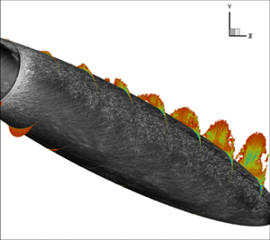
Figure 1 illustrates the qualitative nature of the flow at  $20^\circ$ angle of attack using results from the present simulations. The trip is visible on the left of the image, increasing the skin friction in its wake. The skin friction lines show the turning of the flow towards the leeward side along the length of the spheroid. The three-dimensional boundary layer separates on the leeward side to produce a counter-rotating vortex pair whose strength and size increase along the spheroid length. The vortices entrain freestream fluid that then impinges on the spheroid near the meridian plane. The high pressure due to impingement then redirects the flow towards the windward side underneath the primary vortex. Depending on the Reynolds number, this reversed flow undergoes additional separations, resulting in secondary and tertiary vortices.

Figure 1. Isometric view of the flow around the tripped prolate spheroid at  $20^\circ$ angle of attack. The spheroid surface is shaded by skin friction values. The transverse planes are located at every
  $10\,\%$ of
  $L$ and show the axial velocity.
These vortex pairs have been shown to influence the wall pressure coefficient (Chesnakas & Simpson Reference Chesnakas and Simpson1996) and global loads (Ahn Reference Ahn1992). Since the separation is over a smooth surface, its location is dependent on the flow conditions and local Reynolds number. There exists a critical Reynolds number across which the primary separation line is displaced azimuthally (Ahn Reference Ahn1992). The importance of characterizing the three-dimensional boundary layer transition to understand the flow separation has been discussed by Meier & Kreplin (Reference Meier and Kreplin1980) for the non-tripped case. Several natural transition mechanisms have been identified on the prolate spheroid: streamwise Tollmien–Schlichting instability on the windward side; crossflow instability (Stock Reference Stock2006; Xiao et al. Reference Xiao, Zhang, Huang, Chen and Fu2007; Krimmelbein & Radespiel Reference Krimmelbein and Radespiel2009), which originates from the inflection of the secondary flow velocity profile (Saric & Reed Reference Saric and Reed1989; Nie et al. Reference Nie, Krimmelbein, Krumbein and Grabe2018); and centrifugal instability resulting from the wall-parallel inflection point of the streamlines. These instabilities contribute to the onset of turbulence and the production of turbulent kinetic energy in the attached region, which in turn affect the location of separation.
Past experiments (e.g. Fu et al. Reference Fu, Shekarriz, Katz and Huang1994; Chesnakas & Simpson Reference Chesnakas and Simpson1994, Reference Chesnakas and Simpson1996, Reference Chesnakas and Simpson1997; Wetzel, Simpson & Chesnakas Reference Wetzel, Simpson and Chesnakas1998) have tripped the boundary layer using a combination of wires and azimuthally distributed roughness elements located at 20 % of the length from the nose. It is assumed that a tripped flow results in a fully developed boundary layer at the locations of measurement. However, as underscored by Schlatter & Örlü (Reference Schlatter and Örlü2012), the determination of whether the boundary layer is fully developed or transitional is non-trivial even in a zero-pressure gradient flat plate boundary layer. On the prolate spheroid, there are some indications that at the widely studied Reynolds number based on freestream velocity and spheroid length  $Re_L = U_{\infty }L/\nu = 4.2 \times 10^6$ and at high angle of attack of
  $\alpha = 20^\circ$, some regions of the flow reported in past experimental and numerical investigations may not be fully developed downstream of the trip, and might undergo natural transition. Experimentally, Fu et al. (Reference Fu, Shekarriz, Katz and Huang1994) observed that tripping affected the location of separation and vortical structure at
  $Re_L = 4.2 \times 10^5$, that it had little effect past 70 % of the length, and that the influence of tripping at
  $Re_L$ higher than
  $2.1 \times 10^6$ was uncertain because of transition.
Results from past numerical work are consistent with the importance of predicting the transitional/turbulent state of the boundary layer downstream of the trip. A wall-modelled large-eddy simulation study performed by Hedin et al. (Reference Hedin, Berglund, Alin and Fureby2001) observed that the vortex was closer to the wall because of a mismatch in the location of separation. Fureby & Karlsson (Reference Fureby and Karlsson2009) compared the one-equation eddy-viscosity model (OEEVM), the dynamic Smagorinsky model and the localized dynamic kinetic model, and noted that the OEEVM yielded the earliest separation and largest primary vortex compared to the other models. Constantinescu et al. (Reference Constantinescu, Pasinato, Wang, Forsythe and Squires2002) studied the spheroid flow using Reynolds-averaged Navier–Stokes (RANS) with several variations of the Spalart–Allmaras model and detached-eddy simulation (DES). They presented good agreement with experiments from Chesnakas & Simpson (Reference Chesnakas and Simpson1997) and Wetzel et al. (Reference Wetzel, Simpson and Chesnakas1998) on the attached region, with some variation in the amplitude of the pressure dip from the primary vortex, which depended on the model used. Interestingly, they remarked that the Reynolds averaging may suppress small-scale perturbations and result in errors that are larger for the prolate spheroid flows than other separated flows. These deviations were linked to errors in the assessment of the skin friction, separation and loads. Some indication of the importance of modelling transition has also been shown by Xiao et al. (Reference Xiao, Zhang, Huang, Chen and Fu2007), who used RANS, DES and zonal RANS/large-eddy simulation of the flow around the prolate spheroid. Although the authors did not trip the flow numerically, they presented reasonable agreement with compared tripped experimental results. They concluded that both the pressure coefficient and the skin friction matched experiment better with the model accounting for transition. Recently, Aram, Shan & Jiang (Reference Aram, Shan and Jiang2021) and Aram et al. (Reference Aram, Shan, Jiang and Atsavapranee2022) studied the spheroid flow using RANS both without a trip, and with a Hama strip located at 5 % of the length. They concluded that the trip was ineffective at higher angle of attack, and that part of the prolate spheroid still underwent natural transition.
The objective of the current study is to assess the validity of assuming that the tripped boundary layer of a smooth body at angle of attack results in a fully developed turbulent boundary layer. The influence of the trip is assessed for the flow around a prolate spheroid under conditions similar to those in past experiments, and the flow field is analysed to determine if and how the post-trip boundary layer becomes fully developed until separation. The simulations resolve the same trip as described and utilized by Chesnakas & Simpson (Reference Chesnakas and Simpson1994) to obtain a better reproduction of the downstream flow. This is, to the authors’ knowledge, the first trip-resolved numerical study of the prolate spheroid flow, with a finer numerical resolution than any past computations.
The rest of the paper is organized as follows: The simulation details are described in § 2, followed by the description of the problem in § 3 and a discussion of the results in § 4.
2. Numerical approach
2.1. Coordinate systems
Figures 1 and 2 illustrate the coordinate systems that are used in this study. The first, freestream flow-based system uses  $x_0$,
  $y_0$ and
  $z_0$ as its main axes, where
  $x_0$ is aligned with the freestream velocity. The second coordinate system is based on the major axis of the spheroid, and uses
  $x/L$ varying from
  $0$ at the nose to
  $1$ at the tail of the spheroid, and
  $\phi$, the azimuthal coordinate varying from
  $0^\circ$ at the windward meridian line to
  $180^\circ$ at the leeward meridian line. A third ‘friction line coordinate system’ is denoted by the
  ${FL}$ subscript; it uses the projection of the time-averaged edge velocity vector in a wall-parallel plane,
  $x_{FL}$, the wall-normal vector
  $y_{FL}$, and a vector aligned with the spanwise direction at the edge of the boundary layer,
  $z_{FL}$. This coordinate system changes with
  $x/L$ and
  $\phi$, but does not change with the distance from the wall. The edge friction line frame is used to compare quantities throughout the boundary layer in a fashion similar to a two-dimensional description of the flow over a flat plate. This reference frame can be used only in the attached regions of the spheroid because it uses the edge velocity of the boundary layer. The last coordinate system, referred to as the ‘local streamline frame’ and indicated by the
  ${SL}$ subscript, is based on the time-averaged velocity vector at the considered location,
  $x_{SL}$, the projection of the wall-normal vector in a plane orthogonal to the first component,
  $y_{SL}$, and a spanwise vector
  $z_{SL}$. This system changes with
  $x/L$,
  $\phi$ and wall-normal distance. It is used to rotate the velocity gradient or higher-order quantities to measure perturbations in and out of the axis of the local mean flow.

Figure 2. Schematic of local coordinate systems: red indicates friction line, green indicates streamline.
2.2. Large-eddy simulation formulation
An overbar  $\overline {({\cdot })}$ denotes spatial filtering, while the bracket
  $\langle {\cdot } \rangle$ is used to indicate time averaging. The incompressible, spatially filtered Navier–Stokes equations are solved in a large-eddy simulation formulation:
 $$\begin{gather} \frac{\partial \bar{u}_i}{\partial t} + \frac{\partial}{\partial x_j}(\bar{u}_i \bar{u}_j) =-\frac{\partial \bar{p}}{\partial x_i} + \nu\,\frac{\partial^2 \bar{u}_i}{\partial x_j\,\partial x_j} - \frac{\partial \tau_{ij}}{\partial x_j}, \end{gather}$$
 $$\begin{gather}\frac{\partial \bar{u}_i}{\partial x_i} = 0, \end{gather}$$
where  $u_i$ is the velocity,
  $p$ is the pressure, and
  $\nu$ is the kinematic viscosity. The subgrid stress (SGS)
  $\tau _{ij} = \overline {u_iu_j}-\bar {u}_i\bar {u}_j$ is modelled with the dynamic Smagorinsky model (Germano et al. Reference Germano, Piomelli, Moin and Cabot1991; Lilly Reference Lilly1992). A finite-volume, second-order centred spatial discretization is used, where the filtered velocity components and pressure are stored at the cell centroids, while the face-normal velocities are estimated at the face centres. The equations are marched in time with a second-order Crank–Nicolson scheme. The algorithm has shown good performance for multiple complex flows, such as propeller in crashback (Verma & Mahesh Reference Verma and Mahesh2012; Kroll & Mahesh Reference Kroll and Mahesh2022) and flow over hulls (Kumar & Mahesh Reference Kumar and Mahesh2017; Morse & Mahesh Reference Morse and Mahesh2021). The kinetic energy conservation property of the method (Mahesh, Constantinescu & Moin Reference Mahesh, Constantinescu and Moin2004) makes it suitable for high-Reynolds-number flow such as that presented in this paper. The method was extended by Horne & Mahesh (Reference Horne and Mahesh2019) to allow for overlapping (overset) grids and six degrees of freedom movement. Although the present geometry is stationary, overset grids are used for better grid efficiency by circumventing the need for a one-to-one match between the near-wall region and the far field. In addition, overset grids provide more flexibility in the grid generation process as they allow for the modelling of details such as small trip elements, independently from the spheroid grid.
3. Problem description
A Reynolds number  $Re_L = 4.2 \times 10^6$ is considered at angles of attack
  $10^\circ$ and
  $20^\circ$. Two cases are compared, one with trip and one without. The trip has the same specification as the experiments of Chesnakas & Simpson (Reference Chesnakas and Simpson1994). It consists of 230 cylindrical posts located at
  $x/L = 0.20$, whose diameter is
  $8.76 \times 10^{-4}L$ and height is
  $5.11 \times 10^{-4}L$, where
  $L$ is the length of the prolate spheroid. The posts are resolved using an overset ring grid shown in figure 3. Both cases with and without trip use the same grid for the prolate spheroid, though the former uses an additional level of overset for the post grids.

Figure 3. Wall grid of one of the trip elements.
Figure 4 illustrates the incremental overset levels of refinements that are used to increase the near-wall refinement with limited impact on the overall cell count. The numbers of cells and partitions are indicated in table 1, showing that  $78\,\%$ of the control volumes are in the near-wall region – good grid efficiency enabled by the overset methodology. In addition, the overset capability is used to rotate the grid of the geometry, which specifies the incidence of the flow without having to modify the grid and limit the maximum skewness. The near-wall resolution in wall units is
  $\Delta x^+ = 100$,
  $r \,\Delta \phi ^+ = 20$ and
  $\Delta r^+ = 0.5$. The wall-normal stretching ratio of the boundary layer clustering is
  $1.02$.

Figure 4. Schematic of the three levels of overset grid refinement.
Table 1. Number of control volumes and processors for each overset grid level.

The outer boundary is a cylinder of  $8D$ radius and
  $20D$ length, where
  $D$ is the minor diameter of the spheroid. The blockage ratio is
  $2.2\,\%$, which is considered low enough to neglect confinement effects. Dirichlet boundary conditions are used for the velocity at the inflow. A slip condition is imposed on the remaining far-field boundaries, while a no-slip condition is specified at the wall of the prolate spheroid. The flow fields are interpolated across the boundaries between overset levels in a manner that ensures energy conservation. The overset interpolation is detailed in Horne & Mahesh (Reference Horne and Mahesh2019).
The simulations are time-advanced for  $30 D \,U_{\infty }^{-1}$, where
  $U_{\infty }$ is the velocity at the inflow. This is deemed sufficient when compared to the
  $6 D \, U_{\infty }^{-1}$ necessary for the transient. The statistics are measured for
  $2.4 D \,U_{\infty }^{-1}$. The time step for both tripped and non-tripped cases is
  $2 \times 10^{-4} D \, U_{\infty }^{-1}$. This value is limited by the small cells necessary to resolve the geometry of the trip.
The variables of interest are compared at four locations for  $10^\circ$ angle of attack and five to seven locations for
  $20^\circ$ angle of attack, distributed along two friction lines. Friction line 1 starts at
  $x/L = 0.2$ and
  $\phi = 10^\circ$; friction line 2 starts at
  $x/L = 0.5$ and
  $\phi = 10^\circ$. Friction line 1 was chosen because it starts at the location of the trip and is useful to assess how the forcing evolves downstream; The flow following friction line 2 in the attached region eventually separates and intersects the location of measurement of the vortex at
  $x/L = 0.772$. The measurement locations are indicated in tables 2 and 3 for
  $\alpha = 10^\circ$ and
  $20^\circ$, respectively, and displayed in figure 5. For clarity, only four locations are visualized in profile plots at
  $\alpha = 10^\circ$ (locations 2–5 of table 2) and five locations at
  $\alpha = 20^\circ$ (locations 2–6 of table 3).
Table 2. Location of the measurement of velocity profiles along the two considered friction lines at  $10^\circ$ angle of attack.

Table 3. Location of the measurement of velocity profiles along the two considered friction lines at  $20^\circ$ angle of attack.


Figure 5. Locations of the profiles (blue dots) on friction lines 1 and 2 (red lines).
3.1. Identification of the fully developed turbulent boundary layer
The identification of a fully developed turbulent boundary layer is made based on three metrics: (i) the development of a logarithmic region in the velocity profiles; (ii) the convergence of the energy spectrum toward a common curve along the streamwise direction; (iii) the unsteadiness of the skin friction coefficient. The last metric differs from the other two because it is based on near-wall perturbation and thus allows us to compare the behaviour at the wall with that of the outer region of the boundary layer.
3.2. Grid convergence
A coarse grid containing 225 million control volumes is compared to the fine, 570 million control volume grid in order to estimate the effect of grid refinement on the results. Figure 6 shows the axial component of the instantaneous velocity at  $x/L = 0.772$, along with the mean secondary streamlines at the same location, and wall-pressure coefficient
  $c_p$. The primary separation in the coarse grid is slightly delayed, with a slightly smaller primary vortex. In addition, the axial velocity deficit in the primary vortex is larger in the fine case. The pressure coefficient is similar between the two cases; however, the fine grid shows the signature of the secondary vortex at
  $\phi = 140^{\circ }$, which is not visible on the coarse grid.

Figure 6. Instantaneous axial component of velocity and averaged pressure coefficient at  $x/L = 0.772$ comparing Wetzel (Reference Wetzel1996) (blue circles) and Chesnakas & Simpson (Reference Chesnakas and Simpson1996) (red crosses) with trip, with (a) the coarse grid and (b) the fine grid.
Figure 7 shows the skin friction coefficient  $c_f$ obtained with the coarse and fine grids, both without trip. For both cases, three distinct regions are visible on the midbody: a quiescent region for
  $\phi < 30^\circ$; followed by a perturbed region for
  $30^\circ < \phi < 100^\circ$, showing streamwise streaks; and an unsteady region for
  $\phi > 100^\circ$. For both, the location of primary separation is visible where the direction of
  $c_f$ rotates toward the aft end of the spheroid. Apart from these similarities, some differences are noted: the quiescent region has some diffuse perturbations in the coarse case that are not observed in the fine case; the flow angle in the coarse case is different than in the fine case on the perturbed region; the boundary between the perturbed and unsteady regions is delayed and more clearly defined in the coarse case.

Figure 7. Instantaneous skin friction coefficient for (a) coarse and (b) fine grids without trip.
The velocity profiles in the friction line direction are compared in figure 8, between the coarse and fine grids, without trip. Although the profiles are similar at the beginning of both friction lines, the two cases have differences in both shape and amplitude at the edge of the boundary layer.

Figure 8. Profiles of dimensionless streamwise velocity along (a–e) friction line 1, and (f–j) friction line 2, for the case without trip on the coarse (green) and fine (black) grids. Profiles 2 (a and f) to 6 (e and j) are shown. The dashed lines indicate the location of  $\delta _{99}$ of the coarse (green) and fine (black) grids.
Figure 9 shows the turbulent kinetic energy along both friction lines, for the two cases. Contrary to what was observed on the velocity profiles (figure 8), the largest differences occur on the three middle profiles for each friction line, which corresponds to the perturbed region discussed above. At these locations, the turbulent kinetic energy is higher for the coarse grid.

Figure 9. Profiles of dimensionless resolved turbulent kinetic energy along (a–e) friction line 1, and (f–j) friction line 2, for the case without trip on the coarse (green) and fine (black) grids.
From these observations, it is concluded that the main features of the flow are similar in both the coarse and the fine grid, although there are some quantitative differences between the two. The coarse grid appears overall more unsteady, with stronger levels of turbulence. This suggests that the dampening of these perturbations is not an effect of the subgrid model, although sufficient resolution is necessary to capture the physical process behind it.
4. Results and discussion
4.1. Difference between tripped and non-tripped cases
4.1.1. Vortex pair and pressure
The instantaneous axial velocity for the tripped and non-tripped cases is shown in figure 10. The turbulent separation and formation of the primary vortex pair are visible in both cases. The size and the location of separation and primary vortex are comparable between the two cases. The flow in the centre of the vortex has slightly less momentum in the tripped case compared to its non-tripped counterpart. The pressure coefficient shows good agreement with experiment from  $\phi = 0^\circ$ to
  $\phi = 75^\circ$. There is a global minimum at approximately
  $\phi = 80^\circ$ as the flow accelerates along the side and the pressure gradient changes from favourable to adverse at that location. Experimental comparisons predict a slightly earlier azimuth for the global minimum at approximately
  $\phi = 75^\circ$, followed by an earlier increase in pressure. Another local minimum of pressure is visible at
  $\phi = 160^\circ$, below the primary vortex. This minimum is lower and earlier in
  $\phi$ in experiments compared with the current predictions. Comparing the tripped and non-tripped cases, the pressure coefficient appears similar in amplitude and location of extrema.

Figure 10. Instantaneous axial component of velocity and averaged pressure coefficient at  $x/L = 0.772$ comparing Wetzel (Reference Wetzel1996) (blue circles) and Chesnakas & Simpson (Reference Chesnakas and Simpson1996) (red crosses) in the cases (a) with trip and (b) without trip.
The similarity between the tripped and non-tripped cases indicates that the influence of the trip at this location is negligible. The fact that the flow is unsteady on the windward side of the non-tripped case suggests that the trip is not necessary to achieve boundary layer transition, and that it is not the leading source of instability at this location. The agreement in pressure in the attached region indicates that the freestream flow is predicted correctly.
4.1.2. Skin friction
The instantaneous skin friction is shown for both cases in figure 11 at  $20^\circ$ angle of attack. Strong convection is observed from the windward side to the leeward side. The maximum flow angle with respect to the axis of the spheroid is approximately
  $32^\circ$, over
  $1.5$ times the angle of attack. Two distinct regions are observed, separated by a diffuse boundary at approximately
  $\phi = 100^\circ$. In the region below, the variation of skin friction shows streamwise streaks, while over
  $\phi = 100^\circ$, the skin friction is noisier and the boundary layer flow is more unsteady. Comparing the two cases, the differences are limited to
  $\phi < 30^\circ$. Downstream of this azimuth (i.e. for
  $\phi > 30^\circ$), the skin frictions in the tripped and non-tripped cases have similar values, which suggests that the turbulent state of the boundary layer in this region is not necessarily due to the difference in upstream disturbances.

Figure 11. Instantaneous skin friction coefficient for (a) the tripped case and (b) without trip, at  $20^\circ$ angle of attack.
4.1.3. Boundary layer parameters
Boundary layer parameters are provided in table 4 for the tripped case. All three thicknesses decrease on the windward side before increasing again on the leeward side. On friction line 1, the minimum of  $\delta _{99}$ is at the fifth location, while the minima of displacement thickness
  $\delta ^*$ and momentum thickness
  $\theta$ are at the third location. Apart from the first location (over the trip), the shape factor
  $H = \delta ^* / \theta$ increases until the fifth location with a jump between the third and fourth location, before decreasing until the end of the line. On friction line 2, the minima of all three thicknesses occur earlier, at the second location. The streamwise pressure gradient parameter
  $\beta _1 = \delta ^*/(\rho u_{\tau }^2) \, \partial P_e / \partial x_{SL}$ is favourable on the first four locations of both lines, and adverse on the last three locations. The spanwise pressure gradient parameter
  $\beta _3 = \delta ^*/(\rho u_{\tau }^2) \, \partial P_e / \partial z_{SL}$ is larger in magnitude and follows the opposite trend. The reversal of both pressure gradients occurs close to location 5 on friction line 1, and between locations 4 and 5 on friction line 2.
Table 4. Boundary layer parameters in the case with trip at  $20^\circ$ angle of attack.

Table 5 shows boundary layer parameters in the case without trip. On friction line 1, the thicknesses reach a minimum at the second location, then increase until the end of the line. No decrease of the thicknesses is observed on friction line 2. The shape factor decreases overall on both lines, although a jump is seen at the fourth location of each. Similarly to the tripped case, the spanwise pressure gradient is larger in magnitude than the streamwise pressure gradient, with opposite sign.
Table 5. Boundary layer parameters in the case without trip at  $20^\circ$ angle of attack.

All three metrics of thicknesses provided are larger in the tripped case, particularly on friction line 1, and converge to similar values by the ends of both lines. The larger values show that the effect of the trip is to increase the deficit of momentum close to the wall; the subsequent increase illustrates that the flow recovers from the forcing and converges toward the non-tripped solution. For both cases and both friction lines, the jump in shape factor on the side of the spheroid occurs upstream of the reversal of the streamwise and spanwise components of the pressure gradient. The larger magnitude of the spanwise pressure gradient compared to the streamwise pressure gradient suggests that it is an important factor to consider in studying the evolution of the boundary layer. The jump in adverse streamwise pressure gradient at the last two locations is related to the primary separation that occurs downstream of location 7.
4.1.4. Mean velocity
The friction lines on the wall of the spheroid are shown in figure 12. The regions of convergence are indicative of separation, which show good agreement with Wetzel (Reference Wetzel1996). The azimuth of the primary separation decreases linearly with the axial location from  $x/L = 0.3$ to
  $x/L = 0.85$. The lines have an inflection point between
  $\phi = 60^\circ$ and
  $\phi = 90^\circ$.

Figure 12. Friction lines on the prolate spheroid in the tripped case, compared with experiments from Wetzel (Reference Wetzel1996), who recorded the lines using hot film and oil flow measurements. The red lines indicate friction lines 1 and 2, used for the velocity profile measurements.
Figure 13 shows the streamwise velocity profiles for cases with and without trip at stations along the two friction lines of interest. On friction line 1, the two cases are different at the first two locations. The velocity profiles converge to a common curve at the last three locations. On friction line 2, the profiles from the two cases are laminar at the beginning on the first location and become either transitional or turbulent with increasing distance. The profiles are comparable between tripped and non-tripped cases all along this friction line.

Figure 13. Profiles of dimensionless streamwise velocity along (a–e) friction line 1, and (f–j) friction line 2, for the cases with (red) and without (black) trip, for  $\alpha = 20^\circ$. Profiles 2 (a) to 6 (e) are shown. The dashed lines indicate the location of
  $\delta _{99}$ of the case with (red) and without (black) trips.
Figure 14 shows the wall-normal velocity profile along friction lines 1 and 2. Similar to what was observed in figure 13, the velocity is different at the first location of friction line 1 between the cases with and without trip, although the two profiles converge towards a common curve farther downstream. On friction line 2, the two cases have similar profiles throughout the line. The wall-normal component is positive in the tripped case on friction line 1 between the wall and  $y^+ \approx 200$ at the first three locations, indicating that the flow moves away from the wall. The negative wall-normal velocities in both cases farther from the wall indicate flow attachment from the freestream at the first three locations of friction lines 1 and 2. On the other hand, the wall-normal velocity is positive farther from the wall on the last two locations of both lines, indicative of separation of the boundary layer.

Figure 14. Profiles of dimensionless wall-normal velocity along (a–e) friction line 1, and (f–j) friction line 2, for the cases with (red) and without (black) trip.
Figure 15 shows the spanwise velocity component throughout the boundary layer along friction lines 1 and 2. Positive values of spanwise velocity are indicative of crossflow towards the windward side, while negative values represent a crossflow in the leeward direction. For both lines at the first four locations, a strong crossflow of approximately  $0.06 U_e$ to
  $0.1 U_e$ is observed towards the leeward side at
  $y^+ \approx 20$, with a crossflow in the opposite direction at
  $y^+ > 100$. At the last location of both friction lines, the crossflow is positive close to the wall and negative farther from it.

Figure 15. Profiles of dimensionless spanwise velocity along (a–e) friction line 1, and (f–j) friction line 2, for the cases with (red) and without (black) trip.
Comparison of the velocity components between the two cases on friction line 1 suggests that the disturbance dissipates with increasing distance even though the initial perturbation from the trip is strong. The fact that the tripped boundary layer is similar to the non-tripped counterpart is another indication of stabilization of the boundary layer, which removes the history effect of the trip.
4.1.5. Reynolds stress
Figures 16–18 show the streamwise, wall-normal and spanwise normal Reynolds stresses along the two friction lines. The largest components are in the streamwise direction, followed by the spanwise direction, followed by the wall-normal direction. In addition, the peaks of magnitude of each component occur at different locations:  $y^+ = 10\unicode{x2013}30$ for the streamwise direction,
  $y^+ \approx 100$ in the wall-normal direction, and
  $y^+ = 20\unicode{x2013}100$ with more spread for the spanwise direction. On friction line 1: in the tripped case, for all three components, the magnitude decreases, stagnates and rises again on the leeward side. In the case without trip, the intensities increase between the first two locations, stagnate to match levels similar to the tripped case, then rise again on the leeward side (last two locations). On friction line 2, the intensities are constant, then increase on the leeward side. On this line, similar intensities are observed between the cases with and without trip.

Figure 16. Profiles of dimensionless streamwise Reynolds normal stress along (a–e) friction line 1, and (f–j) friction line 2, for the cases with (red) and without (black) trip.

Figure 17. Profiles of dimensionless wall-normal Reynolds normal stress along (a–e) friction line 1, and (f–j) friction line 2, for the cases with (red) and without (black) trip.

Figure 18. Profiles of dimensionless spanwise Reynolds normal stress along (a–e) friction line 1, and (f–j) friction line 2, for the cases with (red) and without (black) trip.
Figures 19–21 show the three shear components of the Reynolds stress tensor along the two friction lines for both studied cases. The largest values are for the streamwise/spanwise component  $\langle u_{SL}' w_{SL}' \rangle ^+$, followed by the streamwise/wall-normal component
  $\langle u_{SL}' v_{SL}' \rangle ^+$ and the wall-normal/spanwise component
  $\langle v_{SL}' w_{SL}' \rangle ^+$. For the two latter components, the maximum intensity occurs on the leeward side of the prolate spheroid (last two locations); they are negatively correlated and have similar values in the cases with and without trip. For the streamwise/spanwise component
  $\langle u_{SL}' w_{SL}' \rangle ^+$, the maximum intensity is on the side of the spheroid for both friction lines and cases (second, third and fourth locations), and is positively correlated.

Figure 19. Profiles of dimensionless streamwise/wall-normal Reynolds shear stress along (a–e) friction line 1, and (f–j) friction line 2, for the cases with (red) and without (black) trip.

Figure 20. Profiles of dimensionless streamwise/spanwise Reynolds shear stress along (a–e) friction line 1 and (f–j) friction line 2, for the cases with (red) and without (black) trip.

Figure 21. Profiles of dimensionless wall-normal/spanwise Reynolds shear stress along (a–e) friction line 1, and (f–j) friction line 2, for the cases with (red) and without (black) trip.
The decrease of all six components of the Reynolds stress tensor in the tripped case, at the first three locations ( $\phi = 19.4^\circ$ to
  $\phi = 66.0^\circ$) of friction line 1, reinforces the previous observation that disturbances decrease with distance downstream of the trip, on the windward side. The collapse of the two cases on the leeward side of friction line 1 and on friction line 2 is another indication of the erasure of the history effect from the trip.
The normal Reynolds stresses in the streamwise direction are found to be the largest, followed by the spanwise direction, followed by the wall-normal direction. The fact that the spanwise component is so strong also points to the importance of the crossflow to the dynamics of the flow. It is also related to the strong streamwise/spanwise Reynolds shear component, indicative of turbulent eddies aligned with the wall-normal direction.
4.1.6. Turbulent kinetic energy
Figure 22 shows the resolved turbulent kinetic energy (TKE) at five locations along friction lines 1 and 2. For the case with trip, the TKE decreases at the beginning of the first line to reach a minimum at the third location on the side of the spheroid, and increases again on the leeward side (last two locations). The TKE from the case without trip increases from a small value at the first location and becomes constant at a level similar to the tripped case on the second and third locations, before increasing again at the last location. The TKE values of the tripped and non-tripped cases are comparable along friction line 2. For both cases, TKE remains constant on the first half of friction line 2 (windward side), with an increase at the last two locations (leeward side). In both cases, the decrease of TKE is indicative of a dampening of the perturbations on the windward side and is consistent with the observations made on the components of the Reynolds stress tensor.

Figure 22. Profiles of dimensionless resolved TKE along (a–e) friction line 1, and (f–j) friction line 2, for the cases with (red) and without (black) trip, for  $\alpha = 20^\circ$.
The evolution of the production of TKE (as defined in § A.1) displayed in figure 23 follows the same trend as the TKE. Despite the decrease of the energy, the production remains positive though decreasing on the first halves of both friction lines, and increasing on the second halves. In addition, the production term in the tripped case is larger than in the case without trip at the beginning of friction line 1, despite a faster decrease of turbulence with the former. This apparent contradiction is resolved when comparing the relative weight of production of TKE to the maximum viscous dissipation in the boundary layer in figure 24. Indeed, the production to dissipation ratio in the case without trip is over twice as much on the first studied location compared to the case with trip.

Figure 23. Profiles of dimensionless TKE production along (a–e) friction line 1, and (f–j) friction line 2, for the cases with (red) and without (black) trip. A positive value is indicative of a transfer of energy from the mean flow to turbulence levels.

Figure 24. Profiles of dimensionless TKE production non-dimensionalized by maximum viscous dissipation along (a–e) friction line 1, and (f–j) friction line 2, for the cases with (red) and without (black) trip.
4.1.7. Spectra
Figures 25–27 show the spectra of the normal Reynolds stresses along friction lines 1 and 2 at  $1 \times 10^{-3} D$ away from the wall. At the beginning of friction line 1, the spectra of the tripped case have slightly higher intensities than the case without trip in the lower frequency range between 1 and 10 frequency units; however, the magnitude of the non-tripped case drops quickly, starting from 10–50 units, while stronger intensities are observed at high frequency in the tripped case. Farther along friction line 1, the spectra from all three directions collapse onto a similar curve between the two cases. On friction line 2, the largest difference between the two cases is at the first location, where the curve from the tripped case is shifted to higher frequency, although the rate of the drop off is similar to the case without trip. Farther along friction line 2, the spectra from the two cases are similar. In addition, the change in magnitude of the spectra along the friction lines depends on the frequency. The trip is responsible for a broadband spectrum, with higher magnitude in the smaller scales, which decreases with distance along friction line 1. The lower frequencies, on the other hand, conserve their energy. The decrease of the high-frequency components is understood in the context of higher turbulent dissipation acting on the small scales of turbulence, while the preservation of the lower frequency is related to the high turbulent production term seen in figure 23, which feeds energy to the larger eddies of the boundary layer. Although the described behaviour is similar in the three directions, some differences are observed in the rate of decay of the streamwise perturbation (figure 25) compared to the two other components (figures 26 and 27) in both cases, with and without trips. The energy for the streamwise component decreases slowly between 1 and 20 frequency units, while it is constant on the other directions, in this range. On friction line 2, the closeness of the spectra between the cases with and without trip shows further similarity between the two cases, even in term of spectral content. In addition, the evolution of the spectra in the tripped case more closely resembles that from the case without trip, with a gain of energy across the scales. This suggests that the spectral signature of the trip is small on the aft midbody.

Figure 25. Spectra of the streamwise Reynolds normal stress product versus dimensionless frequency unit on (a–e) friction line 1, and (f–j) friction line 2, in the cases with (red) and without (black) trip. Here,  $\mathcal {R}_{xx}^+$ is defined as the Fourier transform of the convolution product of
  $\langle u_{SL} \rangle$ with itself.

Figure 26. Spectra of the wall-normal Reynolds normal stress versus dimensionless frequency unit on (a–e) friction line 1, and (f–j) friction line 2, in the cases with (red) and without (black) trip. Here,  $\mathcal {R}_{yy}^+$ is defined as the Fourier transform of the convolution product of
  $\langle v_{SL} \rangle$ with itself.

Figure 27. Spectra of the spanwise Reynolds normal stress versus dimensionless frequency unit on (a–e) friction line 1, and (f–j) friction line 2, in the cases with (red) and without (black) trip. Here,  $\mathcal {R}_{zz}^+$ is defined as the Fourier transform of the convolution product of
  $\langle w_{SL} \rangle$ with itself.
Figure 28 shows the TKE spectra in the cases with and without trip, along friction line 1. In the tripped case, the spectrum is broadband close to the trip. The higher frequencies lose energy with increasing distance, while small variations at the lower frequencies are observed. In the case without trip, the increase in energy occurs for all the frequencies, with the curves converging towards an asymptotic solution. Higher harmonics at frequencies approximately 15 and 30 are observed in the second spectrum for the case without trip. The evolution of the spectrum of TKE in the case without trip is markedly different to the tripped case. Indeed, the increase in energetic content occurs across all scales in the case without trip. Unlike in the case with trip, the intermediate (10–70 frequency units) and smaller scales gain energy with increasing streamwise distance along the friction line, which is also consistent with higher production to dissipation ratio.

Figure 28. Spectra of TKE versus dimensionless frequency unit along friction line 1 (sorted by decreasing darkness) for the cases (a) with trip, and (b) without trip.
4.2. Effect of subgrid model
Table 6 provides the ratio of the subgrid term to the dissipation term in the TKE equation (cf. § A.1) for the fine grid, for the cases with and without trip. For both cases, the ratio increases overall with distance along friction lines 1 and 2. In the region where the perturbations are attenuated (locations 1, 2, 3 and 4 of both lines), however, the contribution of the subgrid term is approximately four times smaller than the viscous dissipation term. This shows that the observed attenuation of the perturbations is not due to the subgrid term.
Table 6. Ratio of the integral of the SGS term of the TKE equation over the integral of the molecular dissipation term, for the cases with and without trip.

4.3. Effect of pressure gradient
Section 4.1 details how the TKE decreases from  $\phi = 40^\circ$ to
  $\phi = 65^\circ$. Favourable pressure gradients have been shown to decrease the intensity of turbulence, and Launder (Reference Launder1965) found that relaminarization of a two-dimensional boundary layer occurred for a threshold value of the acceleration parameter
  $K_x = ({\nu }/{U_e^2}) ({\partial U_e}/{\partial x_{SL}}) = 3 \times 10^6$. On the prolate spheroid, figure 10 shows that the favourable pressure gradient is the strongest for
  $\phi \in [20^\circ, 65^\circ ]$. The values of the acceleration parameter in the streamwise (
 $K_x$), wall-normal (
 $K_y$) and spanwise (
 $K_z$) directions are calculated and provided in figure 29 in order to estimate the contribution of the pressure gradient to the attenuation of the TKE.

Figure 29. Acceleration parameters  $K_x$ (+),
  $K_y$ (o) and
  $K_z$ (
 $*$) in the cases with (red) and without trip (black) on (a) friction line 1, and (b) friction line 2. A definition of the acceleration parameters is provided in § A.3.
Note that because of conservation of mass, the equality  $K_x + K_y + K_z = 0$ must hold. On the windward side (locations 1–4), the streamwise parameter
  $K_x$ is small compared to
  $K_y$ and
  $K_z$, which have similar values but opposite signs. The wall-normal acceleration parameter
  $K_y$ is negative and increases before reaching a small value at the fifth location. The spanwise parameter, on the other hand, decreases to reach a small value at the fifth location. On the leeward side, both the streamwise and spanwise parameters have similar values and are negative, while the wall-normal component is positive. Figure 29 shows that the pressure gradient parameter in the streamwise direction is smaller than the commonly accepted two-dimensional relaminarization value
  $3 \times 10^{-6}$. The other components of the pressure gradient vector, however, have larger magnitudes than the relaminarization threshold at the beginning of friction line 1. In particular, the spanwise acceleration parameter is positive and thus stabilizes the boundary layer, while the wall-normal pressure gradient is destabilizing. The small values in the streamwise direction compared to the other two directions are an indication that the Launder acceleration parameter is not a reliable metric to assess relaminarization in this flow, since the pressure gradient is strongly three-dimensional and thus outside the scope in which the critical value was established.
For these reasons, the effect of the pressure gradient on the turbulent intensities is assessed in a different manner, by observing its contribution to production terms in the normal directions in comparison to the destabilizing shear production. Figures 30–33 show the contributions  $\mathcal {P}_{12}$,
  $\mathcal {P}_{11}$,
  $\mathcal {P}_{22}$ and
  $\mathcal {P}_{33}$ compared to
  $\|\mathcal {P}\|_2$, where
  $\mathcal {P}_{\alpha \beta } = \langle u_{\alpha }'u_{\beta }' \rangle ({\partial \langle u_{\alpha } \rangle }/{\partial x_{\beta }})$. The production due to shear
  $\mathcal {P}_{12}$ is dominant throughout the boundary layer, with smaller values close to the wall in the tripped case. Here,
  $\mathcal {P}_{11}$ is a sink of TKE on the windward side and a source on the leeward side; it is negligible inside the boundary layer. The negative values of
  $\mathcal {P}_{33}$ on the windward side imply that it is a sink of TKE, while
  $\mathcal {P}_{22}$ is a source. Generally,
  $\mathcal {P}_{11}$,
  $\mathcal {P}_{22}$ and
  $\mathcal {P}_{33}$ are negligible compared to the shear production throughout the boundary layer, except at the edge, where the shear become small and the wall-normal and spanwise terms become larger.

Figure 30. Contribution of the  $xy$ term of the TKE production along (a–e) friction line 1, and (f–j) friction line 2, for the cases with (red) and without (black) trip.

Figure 31. Contribution of the  $xx$ term of the TKE production along (a–e) friction line 1, and (f–j) friction line 2, for the cases with (red) and without (black) trip.

Figure 32. Contribution of the  $yy$ term of the TKE production along (a–e) friction line 1, and (f–j) friction line 2, for the cases with (red) and without (black) trip.

Figure 33. Contribution of the  $zz$ term of the TKE production along (a–e) friction line 1, and (f–j) friction line 2, for the cases with (red) and without (black) trip.
4.4. Effect of streamline line curvature
Finnigan (Reference Finnigan1983) and Morse & Mahesh (Reference Morse and Mahesh2021) derived the Navier–Stokes equations in streamline coordinates, which contain explicit centrifugal terms. The centrifugal terms and pressure gradient can be combined into a corrected pressure gradient as defined in
 \begin{equation} \left(\frac{\partial \langle P \rangle}{\partial y}\right)_{corr} = \frac{\partial \langle P \rangle}{\partial y_{SL}} +\rho\,\frac{\langle u_{SL} \rangle ^2}{R_y}, \quad \left(\frac{\partial \langle P \rangle}{\partial z}\right)_{corr} = \frac{\partial \langle P \rangle}{\partial z_{SL}} + \rho\, \frac{\langle u_{SL} \rangle ^2}{R_z}, \end{equation}
where  $R_y$ and
  $R_z$ are the radii of curvature in the wall-normal and spanwise directions. If the viscous and turbulent stresses are small, then a centrifugal balance can be written in the two directions orthogonal to the streamline such that
  $({\partial \langle P \rangle }/{\partial y})_{corr} = 0$ and
  $({\partial \langle P \rangle }/{\partial z})_{corr} = 0$.
Figure 34 compares the centrifugal acceleration to the pressure gradient in the vicinity of the wall at the second location of friction line 1. Even inside the boundary layer ( $y^+ < 100$), where viscous and turbulent terms are important, the wall-normal balance is dominated by centrifugal effects. In the spanwise direction, the two terms differ for
  $y^+ < 80$, and agree closely farther from the wall. This suggests that the pressure gradient in the wall-normal and spanwise directions originates from the curvature of the streamline. This in turn influences the production term of the TKE equation, as seen in figures 31–33. In addition to these considerations, streamline curvature leads to other effects related to the stability of the boundary layer.

Figure 34. Centrifugal acceleration (purple) and pressure gradient (green) in the (a) wall-normal and (b) spanwise directions, for the case without trip, at the second location of friction line 1. Note that  $R_y$ and
  $R_z$ are negative at this location.
One of these effects, illustrated in figure 35, is to either dampen or amplify turbulence. Consider an eddy with a negative streamwise/wall-normal Reynolds shear stress  $\langle u_{SL}'v_{SL}' \rangle < 0$ along a convex streamwise curvature. If
  $u_{SL}' > 0$, i.e. the centrifugal acceleration is stronger than the wall-normal pressure gradient, then the fluid gains momentum in the wall-normal direction, i.e.
  $v_{SL}' > 0$, and
  $\langle u_{SL}'v_{SL}' \rangle$ becomes less negative. Similarly, if
  $u_{SL}' < 0$, then
  $v_{SL}' < 0$, and
  $\langle u_{SL}'v_{SL}' \rangle$ also becomes less negative. In this case, the streamline curvature dampens turbulence; however, if the streamline curvature or the shear is in the other direction, then the turbulence is amplified. Similarly, spanwise streamline curvature can either decrease or increase
  $\langle u_{SL}'w_{SL}' \rangle$.

Figure 35. Schematic of the stabilization of the boundary layer from a convex streamline curvature. A mean balance exists such that the wall-normal pressure gradient is balanced by the centrifugal acceleration. If a particle has higher streamwise velocity than the mean flow, then the centrifugal acceleration becomes larger than the pressure gradient, creating a positive wall-normal component.
Streamline curvature affects the TKE (A1) in two ways: (i) the change of  $\langle u_{SL}'v_{SL}' \rangle$ and
  $\langle u_{SL}'w_{SL}' \rangle$ modifies the production of TKE
  $\mathcal {P}$; (ii) additional terms are introduced, namely
  $\mathcal {P}_y^c = \langle u_{SL}' v_{SL}' \rangle \langle u_{SL} \rangle /R_y$ and
  $\mathcal {P}_y^c = \langle u_{SL}' w_{SL}' \rangle \langle u_{SL} \rangle / R_z$. Figure 36 shows the production of TKE due to the wall-normal curvature
  $\mathcal {P}_y^c$. It is negative and decreases with distance along both friction lines, implying that the effect of this curvature is to reduce TKE in the boundary layer. The wall-normal curvature does contribute to a diminution of the turbulence kinetic energy; however, the magnitude is small compared to the production term seen in figure 23, especially on the windward side where a decrease of the perturbations is observed. While the explicit contribution of the streamline curvature to the turbulent budget
  $\mathcal {P}_y^c$ is small, it is important to note that the shear production
  $\mathcal {P}_{12}$ is dominant (figure 30) and that the curvature in the wall-normal direction contributes to a reduction of that term via the
  $\langle u_{SL}'v_{SL}' \rangle$ product.

Figure 36. Production term of TKE due to friction line curvature in the wall-normal direction, in the cases with (red) and without (black) trip, along (a–e) friction line 1, and (f–j) friction line 2.
Figure 37 shows the production of TKE due to spanwise curvature. The spanwise curvature term is positive on the first half of both friction lines, then varies between positive and negative at the ends of the lines. The positivity of this term implies that the spanwise curvature is a source of TKE on the windward side. Thus the curvature in the spanwise direction contributes to an increase of TKE on the windward side, and both positive and negative contributions on the leeward side. For the same reason that wall-normal curvature affects  $\langle u_{SL}' v_{SL}' \rangle$, the spanwise curvature is understood as the origin of the large
  $\langle u_{SL}' w_{SL}' \rangle$ values observed in figure 20. On the windward side, perturbations in the streamwise direction are correlated with perturbations in the spanwise direction because of the curvature of the mean flow, such that wall-normal aligned eddies are amplified. On the other hand, figure 19 shows that the
  $\langle u_{SL}' v_{SL}' \rangle$ component remains close to constant and smaller in magnitude than
  $\langle u_{SL}' w_{SL}' \rangle$ despite production from the wall-normal shear. Similarly, the fact that the
  $\langle w_{SL}' w_{SL}' \rangle$ intensity is close to an order of magnitude larger than the
  $\langle v_{SL}' v_{SL}' \rangle$ component is also indicative of turbulence production via streamline curvature.

Figure 37. Production term of TKE due to friction line curvature in the spanwise direction, in the cases with (red) and without (black) trip, along (a–e) friction line 1, and (f–j) friction line 2.
Figure 38 shows the ratio of the spanwise velocity over the streamwise velocity, in the friction line coordinate system. The ratio is negative and increasing with distance from the wall on the first four locations of friction line 1, and the first three locations of friction line 2. The ratio is positive and decreasing with distance from the wall on the last location of both lines. This means that on the windward side, low-momentum fluid close to the wall moves more towards the leeward side, while the velocity vector of high-momentum fluid away from the wall has a stronger axial component, resulting in a secondary flow. This secondary flow is understood as a consequence of a balance between pressure gradient and centrifugal acceleration, which are combined in (4.1) into the corrected pressure gradient. Figure 34 shows both terms of this corrected pressure gradient. In the spanwise direction, the pressure gradient is greater than the centrifugal acceleration for  $y^+ < 30$, which means that
  $(\partial \langle P \rangle / \partial z)_{corr} > 0$, i.e. the fluid is accelerated toward the leeward side close to the wall. The pressure gradient is smaller for
  $y^+ \in [30,80]$, then
  $(\partial \langle P \rangle / \partial z)_{corr} < 0$ and the fluid is accelerated towards the windward side.

Figure 38. Ratio of spanwise velocity to streamwise velocity, in the cases with (red) and without (black) trip, along (a–e) friction line 1, and (f–j) friction line 2.
The same process alters the way the trip functions, as illustrated in figure 39. First, the trip acts as a sink of mean momentum that slows the fluid in the boundary layer. Since  $R_z$ is negative,
  $\rho ({\langle u_{SL} \rangle ^2}/{R_z})$ increases when
  $u_{SL}$ decreases, hence
  $\partial \langle P \rangle / \partial z_{SL}$ increases. This forcing pushes the trip wake to the windward side. This phenomenon is also evidenced by the positive
  $\langle u_{SL}' w_{SL}' \rangle$, showing that a higher
  $u_{SL}'$ velocity perturbation is correlated with a higher
  $w_{SL}'$ perturbation. This reduces the windward area of the spheroid that is in the mean advected wake of the trip. Fransson et al. (Reference Fransson, Brandt, Talamelli and Cossu2004) and Ma & Mahesh (Reference Ma and Mahesh2022) discuss low- and high-speed streaks generated by a trip element in relation to the growth of perturbation leading to transition. In the present case, low- and high-speed streaks are segregated because of the centrifugal balance leading to the former following a streamline along the azimuth, while the latter follow a path closer to the axis of the spheroid. The separation of the low- and high-speed streaks further alters the behaviour of the trip wake flow. In addition, high-momentum fluid is pushed away from the wall because of wall-normal curvature increasing
  $\langle u_{SL}' v_{SL}' \rangle$, while low-momentum fluid is transported towards the wall.

Figure 39. Schematic of the influence of wall-parallel curvature on low- and high-speed flow. (a) Low-speed flow follows higher curvature than high-speed flow because of the centrifugal balance. This also translates into a positive correlation between streamwise and spanwise perturbations. (b) The difference in curvature is responsible for a fanning of the streamlines, such that low-momentum fluid from the trip has a stronger azimuthal velocity component than high-momentum fluid.
In summary, this centrifugal balance in two directions is responsible for: (i) an attenuation or amplification of the perturbations depending on the convexity and the sign of mean shear, where this term appears as an additional source in the TKE equation along streamlines; (ii) a secondary flow in the boundary layer produced by varying streamwise velocity and visible as a non-zero  $w_{FL}$ component.
4.5. Diffusion of the perturbations
Advection and turbulent diffusion reduce the perturbations from the trip, which become insufficient to trigger early transition. A strong convection is observed in figures 12 and 11, transporting fluid from the windward side to the leeward side. In § 4.4, this advection was found to be amplified by wall-parallel curvature effects. The impact of advection is evaluated by releasing a passive scalar from the trip and monitoring the intensity in the downstream boundary layer. The scalar is transported using an advection/diffusion algorithm developed by Muppidi & Mahesh (Reference Muppidi and Mahesh2006), with Schmidt number 1. Although the passive scalar does not account for the more complex effects of transition, including nonlinear growth of the perturbation, and does not account for production or destruction terms, it is an indicator of the mean advection, turbulent and viscous diffusion that perturbations are subject to.
Figure 40 shows the passive scalar intensity along the axial direction, at  $\phi = 0^\circ$,
  $90^\circ$ and
  $180^\circ$. For the three azimuthal lines, it decreases exponentially with the distance. By the midsection at
  $x/L = 0.5$, the passive scalar intensity is only
  $2 \times 10^{-4}$ of the initial density on the side; by
  $x/L = 0.772$, where the transverse view shown in figure 10 is located, the intensity is approximately
  $2 \times 10^{-5}$. The intensity increases again starting from
  $x/L = 0.9$ at
  $\phi = 90^{\circ}$, as the curve crosses the separation line where there is higher concentrations of passive scalar from the reattached flow. The strong fall-off of its concentration in figure 40 points to the fact that advection and diffusion processes render the effect of the trip minimal on the aftmost half of the spheroid. In addition, the smaller production to dissipation ratio observed in the tripped case in figure 24 indicates that the advection and turbulent diffusion terms are stronger in that case. This suggests that not only does the trip increase the production term through increase of the Reynolds shear, its wake is also rapidly advected to the leeward side, leading to a dilution of the perturbations. The shearing of the flow in the streamwise/spanwise direction due to the streamline curvature (figure 20) results in turbulent diffusion in the wall-parallel plane.

Figure 40. Scalar intensity along the length of the spheroid at  $\phi = 0^\circ$,
  $90^\circ$ and
  $180^\circ$.
4.6. Development of turbulent boundary layer
While the discussion so far has been focused on the attenuation of the perturbations on the windward side, there is evidence that the flow becomes fully turbulent farther downstream. The development of a logarithmic region in the velocity profiles (figure 13), the increase of TKE on the leeward side (figure 22), the increase in unsteadiness of the skin friction coefficient at approximately  $\phi = 100^\circ$ (figure 11), and the collapse of the energy spectra at the last two locations of both friction lines (figures 25–28) are all indications of the development of a turbulent boundary layer on the side of the prolate spheroid in both tripped and non-tripped cases. Note that the unsteadiness of the skin friction precedes the development of a logarithmic region and the collapse of the spectra.
The mechanisms of instability that initiate the growth of the perturbations on the side of the spheroid are related to the streaks seen in the skin friction map (figure 11). Figure 41(a) shows a line used to perform a one-dimensional spatial Fourier transform of the skin friction coefficient  $c_f$. The spectrum is shown in figure 41(b). The peak at wavelength
  $55^{-1}D$ corresponds to the spanwise streaks observed on the skin friction maps. The fact that both cases, with and without trip, have these streaks indicates that this effect is independent of the trip. Indeed, the streaks at
  $\phi \in [30^\circ, 90^\circ ]$ are consistent with crossflow instabilities (Saric & Reed Reference Saric and Reed1989) in that region. Chesnakas & Simpson (Reference Chesnakas and Simpson1994) have observed that the boundary layer is skewed since the near-wall flow velocity has a strong
  $\phi$ component, while the velocity at the edge of the boundary layer has a stronger
  $x$ component. This strong crossflow is also visible in figure 15, which shows that the magnitude of the secondary velocity is as high as
  $10\,\%$ of the freestream velocity.

Figure 41. (a) Measurement of location of the one-dimensional spatial spectrum of skin friction magnitude (indicated by a red line). (b) One-dimensional spatial spectrum of skin friction magnitude versus wavenumber.
4.7. Effect of angle of attack
Figure 42 shows the skin friction coefficient at  $10^\circ$ angle of attack. In the tripped case, the flow is unsteady at all locations for
  $x/L > 0.2$; the near-wall flow looks nearly uniformly perturbed. In the case without trip, the near-wall flow is unperturbed on the windward side on a triangular region bounded by
  $(x/L,\phi ) = (0,0^\circ )$,
  $(0.4,0^\circ )$ and
  $(0,180^\circ )$, and perturbed outside of this region. The unsteady region is visibly similar in both cases, although it starts at an earlier axial location on the windward side, in the case with trip. This indicates that for the smaller angle of attack, the effect of the trip is to introduce unsteadiness in the near-wall flow at a location earlier than otherwise observed in the case without trip. The skin friction map shows less variation in the
  $10^\circ$ case compared to the
  $20^\circ$ case (figure 11). It is unsteady at all locations with
  $x/L > 0.2$, even on the windward side, unlike at
  $\alpha = 20^\circ$, which showed a more quiescent region for
  $\phi < 90^\circ$.

Figure 42. Instantaneous skin friction coefficient for (a) the tripped case, and (b) without trip, at  $10^\circ$ angle of attack.
Figure 43 shows the streamwise velocity profiles on the two considered friction lines. In the case with trip, a logarithmic layer is visible, starting at  $y^+ \approx 30$ for all the locations. The size of this logarithmic region increases with streamwise distance. In the case without trip and on friction line 1, the velocity profile suggests that the boundary layer is laminar at the first location. The curves in the case without trip subsequently collapse to their tripped counterpart. A small logarithmic region is observed starting from the second location of friction line 1 in the case without trip. On friction line 2, the profile from the case without trip is similar to the one with trip, and also shows an increasing large logarithmic region. The presence of logarithmic regions in figure 43 upstream of separation is one of the criteria used to identify a turbulent boundary layer.

Figure 43. Profiles of dimensionless streamwise velocity along (a–d) friction line 1, and (e–h) friction line 2, for the cases with (red) and without (black) trip, for  $\alpha = 10^\circ$.
Figure 44 shows the TKE along the two considered friction lines for  $10^\circ$ angle of attack. In the tripped case, on friction line 1, the TKE increases slightly from
  $k^+ = 10$ to
  $k^+ = 15$, with a larger increase on the last location. In the case without trip, the TKE is small on the first location and increases to match the value of the case with trip in the three locations downstream. The TKE is similar between the two cases on all four locations of friction line 2. It is constant at around
  $k^+ = 11$ on the first three locations, and increases to
  $k^+ = 28$ on the last location. In contrast to the
  $20^\circ$ tripped case, where TKE decreases, the TKE increases slightly post-tripping. Both these observations indicate that the attenuation of the perturbations on the windward side depends on the angle of attack. The fact that it is turbulent earlier in the tripped case than in the case without trip on friction line 1 suggests that the effect of the trip is to trigger early transition. In addition, skin friction, velocity profiles and TKE all have similar values in both cases in the turbulent region. The indicates that there is no over-tripping of the boundary layer. In accordance with the discussed metrics, it is deemed that successful tripping is achieved at
  $10^\circ$ angle of attack.

Figure 44. Profiles of dimensionless resolved TKE along (a–d) friction line 1, and (e–h) friction line 2, for the cases with (red) and without (black) trip, for  $\alpha = 10^\circ$.
Sections 4.3 and 4.4 discuss the idea that pressure gradient and curvature limit the effect of the trip at  $20^\circ$ angle of attack. These effects are thus expected to be reduced at
  $10^\circ$ since the trip is effective for this lower angle of attack. The dimensionless pressure gradient in three directions is shown in figure 45, for
  $10^\circ$ and
  $20^\circ$ angle of attacks. As observed in figure 34, this quantity in the wall-normal and spanwise directions is close in value to the radii of curvature in the edge of the boundary layer. In all three directions, the pressure gradient/streamline curvature is much stronger at
  $\alpha = 20^\circ$ compared to
  $\alpha = 10^\circ$. The fact that these parameters are both reduced in this region at smaller angle of attack is consistent with the idea stated previously that these parameters play a role in the attenuation of the perturbations on the windward side. Similarly, the absence of skin friction streaks at
  $10^\circ$ (figure 42) compared to those observed at
  $20^\circ$ (figure 11) suggests an association between the streaks and the curvature effects.

Figure 45. Dimensionless pressure gradient at the edge of the boundary layer on friction line 1 in the (a) streamwise, (b) wall-normal and (c) spanwise directions, for  $\alpha = 10^\circ$ (black) and
  $\alpha = 20^\circ$ (red), in the case without trip.
4.8. Regime map of the skin friction coefficient at  $20^\circ$ angle of attack

Figure 46 summarizes the interpretation of the near-wall flow topology from the current results. In region A, upstream of the trip, the flow is laminar and transitions naturally in the presence of an adverse pressure gradient. This perturbed boundary layer then flows into region B. Directly downstream of the trip, the skin friction is maximum, with a wake-like flow strongly affected by the roughness elements. Fluid is advected from region C and the freestream into region D. That area is also trip-dependent, and shows variations between the tripped and non-tripped cases. These variations are attenuated, so much that the flow becomes trip-independent by the top interface of that region. Downstream, region E is marked by a strong secondary component of velocity ( $10\,\%$ of freestream velocity) creating crossflow instability that manifests itself as streamwise streaks. The bottom of region F is characterized by development of turbulence followed by primary separation at the top of this area. The flow from the separated boundary layer travels with the primary vortex, where it is reattached at the top border of region H at
  $\phi = 180^\circ$. The unsteady flow travels along the negative
  $\phi$ direction before separating at the bottom border of that region. The secondary vortex is reattached in the middle of region I. This region is characterized by a turbulent boundary layer located underneath the primary and secondary vortices, both of which drive the pressure in the area. Finally, regions G and J were not discussed in the current study and are located on the aft windward and leeward sides of the spheroid, respectively, where the curvature of the wall becomes larger and the pressure gradient along the spheroid axis reverses. Region G has an adverse pressure gradient, with higher skin friction, and looks unsteady. Although both tripped and non-tripped cases show similar behaviour in this location, the former has a larger area. This could be attributed to the earlier transition from the disturbance created by the trip. Region J, on the other hand, has a favourable pressure gradient that relaminarizes the boundary layer and leads to a decrease in unsteadiness and smaller values of skin friction. Experimentally, the spheroid is attached by a sting on the aft of the geometry, which was not accounted for in the current results. The effect of the sting on the flow in regions G and J has not been studied.

Figure 46. Map of the wall flow regions around the prolate spheroid as observed on the instantaneous skin friction coefficient for the tripped case. A: pre-trip laminar region showing advection of disturbances. B: pre-trip unsteady. C: trip wake region. D: windward, freestream impingement and trip-dependent region with attenuation of the perturbations. E: crossflow and pressure gradient reversal region. F: transition to turbulence and primary separation. G: windward stern adverse pressure gradient and transition. H: unsteady primary vortex impingement and secondary separation. I: unsteady, sub-vortex and secondary reattachment region. J: leeward stern relaminarization. Black and red dotted line: primary separation. Green and red dotted line: meridian reattachments. Blue and red dotted line: secondary separation. The black arrows show the direction of the flow across the interfaces.
5. Conclusion
Wall-resolved and trip-resolved large-eddy simulation was used to study the effect of tripping on the prolate spheroid at  $10^\circ$ and
  $20^\circ$ angles of attack, in conditions representative of the experiments of Chesnakas & Simpson (Reference Chesnakas and Simpson1994). Comparison between the flow with and without trip showed that at large angle of attack, the effect of the trip on the transverse flow at
  $x/L = 0.772$ was negligible. Several mechanisms were identified to explain the limited effect from the trip: (i) an attenuation of the initial disturbance from the trip due to pressure gradient, streamline curvature effects; (ii) a strong advection and diffusion of the perturbation limiting the region of influence of the trip. The advection of the trip wake is amplified by wall-normal and wall-parallel curvatures that are responsible for a secondary flow moving low-momentum fluid to the leeward side at a higher angle. Streamline curvatures are also associated with instabilities in the spanwise direction, streaks visible on the skin friction, and large
  $\langle u_{SL}' w_{SL}'\rangle$ values. The boundary layer subsequently becomes fully turbulent downstream of the primary separation. This influences the location of separation and the topology of the primary vortex pair.
The state of the attached boundary layer determines the location of separation, which in turn influences the size and location of the counter-rotating vortex pair and the global loads on the spheroid. For this reason, the occurrence of transition on the tripped prolate spheroid has implications for the macroscale topology of the flow and the prediction of the loads. The present work underscores the importance of windward measurements and accounting for transition even for tripped flows.
Supplementary movie
Supplementary movie is available at https://doi.org/10.1017/jfm.2023.175.
Acknowledgements
We acknowledge N. Morse and T. Kroll for their help, and Dr S. Anantharamu for the grid preprocessor. Computing resources were provided through a United States Department of Defense (DoD) Frontier project of the High Performance Computing Modernization Program (HPCMP) by the US Army Engineer Research and Development Center (ERDC) in Vicksburg, Mississippi, on the Onyx supercomputer of the High Performance Computing Modernization Program, the Texas Advanced Computing Center (TACC) through the Extreme Science and Engineering Discovery Environment (XSEDE) allocation, and the Minnesota Supercomputing Institute (MSI) at the University of Minnesota.
Funding
This work is supported by the US Office of Naval Research (ONR) under ONR grant N00014-20-1-2717, with Dr P. Chang as technical monitor.
Declaration of interests
The authors report no conflict of interest.
Appendix A
A.1. Resolved kinetic energy equation
The equation for the resolved TKE  $k$ is used in the current study to study the mechanisms of amplification or attenuation of the perturbations. It can be derived in a non-inertial frame of reference (such as the streamline reference frame) as
 \begin{gather} \frac{\partial k}{\partial
t}\,{\rm (I)}+\langle u_j \rangle\,\frac{\partial
k}{\partial x_j}\,{\rm (II)}
=-\frac{1}{\rho}\,\frac{\partial}{\partial x_i}\langle u_i'
P' \rangle\,{\rm (III)} +
\nu\, \frac{\partial^2 k}{\partial
x_j\,\partial x_j}\,{\rm (IV)}\nonumber\\
-\frac{\partial }{\partial x_j}\left\langle
\frac{1}{2}\,u_i' u_i' u_j' \right\rangle {\rm (V)} -
\langle u_i'u_j' \rangle\,\frac{\partial \langle u_i
\rangle}{\partial x_j}\,{\rm (VI)} - \nu
\left\langle \frac{\partial u_i'}{\partial
x_j}\,\frac{\partial u_i'}{\partial x_j} \right\rangle {\rm
(VII)} - \left\langle u_i'\, \frac{\partial}{\partial
x_j}\left(\nu_t'\,\frac{\partial u_i'}{\partial x_j}\right)
\right\rangle {\rm (VIII)}\nonumber\\ - \left(\langle
u_{SL}' u_2' \rangle\,\frac{\langle u_{SL} \rangle}{R_y} +
\langle u_{SL}' u_3' \rangle\,\frac{\langle u_{SL}
\rangle}{R_z} +\frac{\langle u_{SL}' u_{SL}'
u_2'\rangle}{R_y} +\frac{\langle u_{SL}' u_{SL}'
u_3'\rangle}{R_z}\right) {\rm (IX)},
\end{gather}
\begin{gather} \frac{\partial k}{\partial
t}\,{\rm (I)}+\langle u_j \rangle\,\frac{\partial
k}{\partial x_j}\,{\rm (II)}
=-\frac{1}{\rho}\,\frac{\partial}{\partial x_i}\langle u_i'
P' \rangle\,{\rm (III)} +
\nu\, \frac{\partial^2 k}{\partial
x_j\,\partial x_j}\,{\rm (IV)}\nonumber\\
-\frac{\partial }{\partial x_j}\left\langle
\frac{1}{2}\,u_i' u_i' u_j' \right\rangle {\rm (V)} -
\langle u_i'u_j' \rangle\,\frac{\partial \langle u_i
\rangle}{\partial x_j}\,{\rm (VI)} - \nu
\left\langle \frac{\partial u_i'}{\partial
x_j}\,\frac{\partial u_i'}{\partial x_j} \right\rangle {\rm
(VII)} - \left\langle u_i'\, \frac{\partial}{\partial
x_j}\left(\nu_t'\,\frac{\partial u_i'}{\partial x_j}\right)
\right\rangle {\rm (VIII)}\nonumber\\ - \left(\langle
u_{SL}' u_2' \rangle\,\frac{\langle u_{SL} \rangle}{R_y} +
\langle u_{SL}' u_3' \rangle\,\frac{\langle u_{SL}
\rangle}{R_z} +\frac{\langle u_{SL}' u_{SL}'
u_2'\rangle}{R_y} +\frac{\langle u_{SL}' u_{SL}'
u_3'\rangle}{R_z}\right) {\rm (IX)},
\end{gather}
where (I) is the temporal variation of TKE, (II) is the advection of  $k$ with the mean flow, (III) is the pressure diffusion term, (IV) is the molecular diffusion of
  $k$, (V) is the turbulent diffusion of
  $k$, and (VI) is the production term, contributing to an increase of TKE if the shear and Reynolds stress tensor term have opposite signs. The latter term also appears in the mean kinetic budget and is thus understood as a transfer term between the two equations. For convenience, the production term is written as
  $\mathcal {P}$. (VII) is the molecular dissipation term, which is always strictly negative or zero; it is written as
  $\epsilon$. (VIII) is the contribution of the SGS to the turbulent kinetic budget, written as
  $\mathcal {D}_{SGS}$. (IX) are additional production terms due to the curvature of the streamline (Bradshaw Reference Bradshaw1973). Here,
  $R_2$ and
  $R_3$ are the radii of curvature in the wall-normal and spanwise directions; they are signed with the direction of curvature with respect to the sign of the shear, and are calculated as
  $R_i^{-1} = \langle u_{SL} \rangle ^{-1} ( \varOmega _k + \partial u_{SL} / \partial x_i)$, where
  $k$ is the index corresponding to the direction orthogonal to the streamline vector and the
  $i$ component (Morse & Mahesh Reference Morse and Mahesh2021). Each term can be either positive or negative, i.e. be a source or a sink of TKE. The triple-product terms are small compared to the Reynolds stress terms and are thus neglected. The production terms due to curvature are written as
  $\mathcal {P}_x^y$ and
  $\mathcal {P}_x^z$.
A.2. Estimation of boundary layer integral quantities
The determination of several metrics used in the present work assumes knowledge of some measure of boundary layer thickness. This measurement is complicated by the fact that the flow velocity is not constant outside the boundary layer. This problem has been a topic of research in the past. Griffin, Fu & Moin (Reference Griffin, Fu and Moin2021) proposed a methodology to estimate the boundary layer thickness in general flows in a manner that remains consistent with the definition for the flow over a flat plate with zero-pressure gradient. The authors consider the potential velocity
 \begin{equation} U_{p} \equiv \sqrt{2\,\frac{P_0-P}{\rho}}, \end{equation}
where  $P_0$ is the pressure at the stagnation point, and
  $P$ is the pressure at the measurement location. The
  $n$th percentile boundary layer thickness can then be defined as the location closest to the wall where
  $U_{p}/U < n/100$, where
  $U$ is the velocity magnitude at the measurement location.
In the case of the prolate spheroid, the stagnation pressure is difficult to obtain numerically. Instead, the potential velocity is obtained using the location of the profile that maximizes the velocity magnitude:
 \begin{equation} U_{p} \equiv \sqrt{2\,\frac{P_{max}-P}{\rho} + U_{max}^2}. \end{equation}
Figure 47 shows a comparison between the two velocities. Despite the fact that the velocity is not constant outside the boundary layer, the computed velocity is a very good approximation of the actual velocity in the potential region.

Figure 47. Calculated potential velocity  $U_p$ (green) and measured velocity magnitude (purple) versus wall-normal coordinate, for the case without trip.
Other integral quantities may then be obtained from this definition, including the displacement thickness  $\delta ^*$, the momentum thickness
  $\theta$, and the shape factor
  $H = \delta ^* / \theta$, as well as
  $Re_{\theta }$ based on momentum thickness and freestream velocity, the streamwise pressure gradient parameter
  $\beta _1 = ({\delta ^*}/{\tau _w}) ({\partial P_e}/{\partial x_{SL}})$ (where
  $P_e$ is the pressure at
  $y_{FL} = \delta _{99}$) and the spanwise pressure gradient parameter
  $\beta _3 = ({\delta ^*}/{\tau _w}) ({\partial P_e}/{\partial z_{SL}})$. In addition, the direction set by the velocity vector at
  $\delta _{99}$ can then be used as a reference to create the friction line coordinate system.
A.3. Acceleration parameters
Launder (Reference Launder1965) observed that relaminarization of a turbulent boundary layer flat plate in favourable pressure gradient occurs for values of the acceleration parameter  $K_x > 3 \times 10^{-6}$ with
 \begin{equation} K_x= \frac{\nu}{U_e^2}\,\frac{\partial U_e}{\partial x_{SL}}, \end{equation}
where  $U_e$ is the edge velocity in the streamwise direction. The pressure gradients in the wall-normal and spanwise directions are extended in the current study and defined as
 \begin{equation} K_y = \frac{\nu}{U_e^2}\,\frac{\partial V_e}{\partial y_{SL}}, \quad K_z = \frac{\nu}{U_e^2}\,\frac{\partial W_e}{\partial z_{SL}}. \end{equation}
The idea behind this generalization is to use the components of the velocity gradient tensor that appear in the normal production terms of TKE,  $\mathcal {P}_{22}$ and
  $\mathcal {P}_{33}$. The gradients
  $\partial V_e/\partial y_{SL}$ and
  $\partial W_e/\partial z_{SL}$ modulate the normal components of the Reynolds stress tensor and are, depending on their sign, a source or a sink of TKE. Note that while the acceleration parameter is a convenient tool to assess the relaminarization due to pressure gradient, it is based on a two-dimensional boundary layer without streamline curvature.


 Open access