


1. Introduction
A direct result of the pressure difference between the suction and pressure sides of a finite-span wing is the formation of wing-tip vortices and their induced three-dimensionality. Despite the formation of these vortices near the tip, they exert a global influence, affecting the entire span of the wing and giving rise to a complex, three-dimensional (3-D) flow.
The most significant impact of the wing-tip vortices on the flow is their induced downwash on the wing, i.e. an induced inviscid velocity normal to the free stream in the downward direction (cf. Houghton et al. Reference Houghton, Carpenter, Collicott and Valentine2013). As illustrated in figure 1, this downwash changes the free-stream direction, reducing the effective angle of attack and consequently the lift, while altering the pressure distribution in the process. The change in the pressure distribution (and thus the streamwise pressure gradient) significantly impacts the development of the boundary layers. In addition, as the induced downwash is inversely proportional to the distance from the vortex core (refer to the caption of figure 1), different spanwise locations on the wing encounter varying free-stream directions and a non-uniform pressure distribution along the span. Note that this is a simplified explanation valid for the geometry of figure 1, but the conclusion is generally valid for other wing configurations (cf. Houghton et al. Reference Houghton, Carpenter, Collicott and Valentine2013). This leads to a spanwise pressure gradient which varies across the chord and span, a non-zero spanwise acceleration and the formation of boundary layers that exhibit 3-D behaviour, such as skewed velocity profiles, across a large portion of the wing's span. This non-zero and variable spanwise velocity introduces additional complexities to the boundary layers, which are added to those already present due to adverse or favourable streamwise pressure gradients (cf. Spalart & Watmuff Reference Spalart and Watmuff1993; Perry, Marusic & Jones Reference Perry, Marusic and Jones2002; Aubertine & Eaton Reference Aubertine and Eaton2005; Monty, Harun & Marusic Reference Monty, Harun and Marusic2011; Harun et al. Reference Harun, Monty, Mathis and Marusic2013; Bobke et al. Reference Bobke, Vinuesa, Örlü and Schlatter2017; Bross, Fuchs & Kahler Reference Bross, Fuchs and Kahler2019; Devenport & Lowe Reference Devenport and Lowe2022; Pozuelo et al. Reference Pozuelo, Li, Schlatter and Vinuesa2022), as well as spanwise pressure gradients and other 3-D effects (cf. Johnston Reference Johnston1960; Perry & Joubert Reference Perry and Joubert1965; van den Berg Reference van den Berg1975; Rotta Reference Rotta1979; Pierce, McAllister & Tennant Reference Pierce, McAllister and Tennant1983; Bradshaw & Pontikos Reference Bradshaw and Pontikos1985; Spalart Reference Spalart1989; Moin et al. Reference Moin, Shih, Driver and Mansour1990; Degani, Smith & Walker Reference Degani, Smith and Walker1993; Ölçmen & Simpson Reference Ölçmen and Simpson1995; Johnston & Flack Reference Johnston and Flack1996; Coleman, Kim & Spalart Reference Coleman, Kim and Spalart2000; Kannepalli & Piomelli Reference Kannepalli and Piomelli2000; Schlatter & Brandt Reference Schlatter and Brandt2010; Kevin & Hutchins Reference Kevin and Hutchins2019; Suardi, Pinelli & Omidyeganeh Reference Suardi, Pinelli and Omidyeganeh2020; Devenport & Lowe Reference Devenport and Lowe2022).

Figure 1. The impact of wing-tip vortices on the effective angle of attack and induced drag. (a) Vortex with strength (circulation)  $\varGamma _{vort}$ induces a downward velocity (downwash) of
 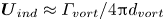 $\boldsymbol {U}_{ind}\approx \varGamma _{vort}/4{\rm \pi} d_{vort}$ (where
  $d_{vort}$ is the distance along the span to the vortex core) on the wing (cf. Houghton et al. Reference Houghton, Carpenter, Collicott and Valentine2013). (b) Change in the effective angle of attack and generation of a new component of drag,
  $\boldsymbol {F}_{lift,x}$, as a result of deflection of the effective free-stream direction,
  $\boldsymbol {U}_{eff}$, compared with the geometric free-stream direction,
  $\boldsymbol {U}_\infty$.
The goal here is to better understand the flow in the vicinity of the wing, and in particular, how the turbulent boundary layers are influenced by the induced three-dimensionality of the finite-span geometry and the resulting wing-tip vortices. This is done by identifying the behaviours present in the finite-span wings which are absent in the limit of infinite span. To do this, a set of high-fidelity simulations is carried out for wings with a symmetric NACA0012 profile and rounded wing-tip geometry at a chord-based Reynolds number of  $Re_c=U_\infty c/\nu =200\,000$ (where
  $U_\infty$ is the free-streem velocity,
  $c$ is the chord and
  $\nu$ is the kinematic viscosity). Free-flight conditions are considered at angles of attack of
  $\alpha =0^\circ$,
  $5^\circ$ and
  $10^\circ$. Additionally, another set of simulations is performed for infinite-span (i.e. periodic) wings with the same profile, Reynolds number and angle of attack, including an additional configuration of
  $\alpha =2^\circ$, which matches the near-root effective angle of attack of the finite-span wing at
  $\alpha =5^\circ$. The boundary layers of the finite-span and infinite-span wings are then compared, the discrepancies are identified and explanations are proposed for the observed differences as well as the underlying mechanisms responsible for them.
The primary focus is on the differences between the finite- and infinite-span wings; thus, common behaviours such as the response to favourable and adverse pressure gradients are excluded from this study. Furthermore, we limit our scope to the regions of the wing which are not dominated by wing-tip vortices or trailing-edge effects. For instance, the flows on the suction and pressure sides of the wing have opposing spanwise components (directed towards the root on the suction side and towards the tip on the pressure side). At the trailing edge, these flows (with different spanwise, streamwise and wall-normal velocity components) intersect, leading to additional shear and vorticity which could influence both the upstream boundary layers and the downstream wake. Similarly, closer to the tip, especially on the suction side, there are stronger 3-D effects and secondary flows present at a more local scale in close vicinity of the wing-tip vortex. The focus here is on regions of the wing that are not dominated by these effects.
Although not directly related to this work, it is worth noting that wing-tip vortices contribute to an additional drag component, known as the induced drag (also called lift-induced drag, or vortex drag; see Houghton et al. Reference Houghton, Carpenter, Collicott and Valentine2013; Federal Aviation Administration 2016). A brief explanation of this is provided in the caption of figure 1. More detailed discussions about this phenomenon, including potential methods to mitigate its effects, can be found in Houghton et al. (Reference Houghton, Carpenter, Collicott and Valentine2013), Federal Aviation Administration (2016), Kroo (Reference Kroo2001), Ceron-Munoz et al. (Reference Ceron-Munoz, Cosin, Coimbra, Correa and Catalano2013) and Phillips, Hunsaker & Joo (Reference Phillips, Hunsaker and Joo2019).
Moreover, this work does not present an in-depth study of the structure of wing-tip vortices, their formation, development and downstream influence. A wealth of research has been dedicated to these topics and is readily available in the literature. A few significant studies worth highlighting here include the work of Spalart (Reference Spalart1998, Reference Spalart2008), focusing on the development of these vortices in the far wake of an aircraft, and studies by Devenport et al. (Reference Devenport, Rife, Liapis and Follin1996), Chow, Zilliac & Bradshaw (Reference Chow, Zilliac and Bradshaw1997a,Reference Chow, Zilliac and Bradshawb) and Giuni & Green (Reference Giuni and Green2013) mainly exploring the near-wake behaviour of these vortices in more canonical settings. Other interesting works include studies into the meandering motion of these vortices for rigid and stationary wings (Dghim et al. Reference Dghim, Miloud, Ferchichi and Fellouah2021), the impact of the heaving motion of the wing on the structure and development of the wing-tip vortices (Fishman, Wolfinger & Rockwell Reference Fishman, Wolfinger and Rockwell2017; Garmann & Visbal Reference Garmann and Visbal2017), the interactions of wing-tip vortices with other co-rotating or counter-rotating vortices (Devenport, Zsoldos & Vogel Reference Devenport, Zsoldos and Vogel1997; Devenport, Vogel & Zsoldos Reference Devenport, Vogel and Zsoldos1999) and the interaction of streamwise-oriented vortices (e.g. wing-tip vortices) upon their incidence on other downstream aerodynamic surfaces (cf. Rockwell Reference Rockwell1998; Garmann & Visbal Reference Garmann and Visbal2015; McKenna, Bross & Rockwell Reference McKenna, Bross and Rockwell2017). We are not aware of any work specifically investigating the influence of the wing-tip vortices on the turbulent boundary layers formed on the wings, which motivated the present study.
The remainder of the paper is structured as follows. Section 2 details the numerical set-up, including the solver, computational domain, boundary conditions, grid and other parameters. The approach for obtaining accurate statistics is also outlined in this section, with more details provided in Appendix A. Section 3 describes the general flow field and its most important features, and § 4, which is the main focus of this work, takes a closer look at the impact of finite span and three-dimensionality on the turbulent boundary layers. Finally, § 5 summarises the findings, acknowledges the limitations and discusses potential future directions.
2. Numerical set-up
2.1. Numerical solver
The numerical solutions presented in this paper are obtained by solving the incompressible Navier–Stokes equations,
 \begin{equation} \frac{\partial u_i}{\partial t}+ u_j \frac{\partial u_i}{\partial x_j} ={-}\frac{1}{\rho}\frac{\partial p}{\partial x_i} + \nu \frac{\partial^{2} u_i }{\partial x_j \partial x_j} , \end{equation}
under the divergence-free constraint,  $\partial u_i / \partial x_i=0$, where
  $u_i$ and
  $p$ are the instantaneous velocity and pressure fields,
  $x_i$ and
  $t$ are the spatial coordinates and time and
  $\rho$ and
  $\nu$ are the fluid density and kinematic viscosity.
These equations are discretised in space and integrated in time using the high-order solver Nek5000, developed by Fischer, Lottes & Kerkemeier (Reference Fischer, Lottes and Kerkemeier2010), with adaptive mesh refinement (AMR) capabilities developed at KTH (Peplinski et al. Reference Peplinski, Offermans, Fischer and Schlatter2018; Offermans Reference Offermans2019; Offermans et al. Reference Offermans, Peplinski, Marin and Schlatter2020; Tanarro et al. Reference Tanarro, Mallor, Offermans, Peplinski, Vinuesa and Schlatter2020). Nek5000 is based on the spectral-element method (Patera Reference Patera1987), essentially a high-order finite-element method, which combines the flexibility of the finite-element formulation in meshing complex geometries with the numerical accuracy of spectral methods (Deville, Fischer & Mund Reference Deville, Fischer and Mund2002). Inside each element, the velocity field is represented by a polynomial of order  $q$ (here
  $q=7$ in all cases) using Lagrange interpolants on the Gauss–Lobatto–Legendre (GLL) points (
 $N=q+1$ GLL points in each direction), while the pressure is represented on
  $q-1$ Gauss–Legendre points following the
  $P_N-P_{N-2}$ formulation (Maday, Patera & Rønquist Reference Maday, Patera and Rønquist1987). The nonlinear convective term is overintegrated on a grid with
  $3N/2$ Gauss–Legendre points in each direction, to avoid (or reduce) aliasing errors. Time stepping is performed by an implicit third-order backward-differentiation scheme for the viscous terms and an explicit third-order extrapolation for the nonlinear terms (Karniadakis, Israeli & Orszag Reference Karniadakis, Israeli and Orszag1991). A high-pass filter relaxation term (Schlatter, Stolz & Kleiser Reference Schlatter, Stolz and Kleiser2004) is added to the right-hand side of the Navier–Stokes equations. This term provides numerical stability and acts as a subgrid-scale dissipation. This specific set-up has been used and verified in several previous studies (Schlatter et al. Reference Schlatter, Li, Brethouwer, Johansson and Henningson2010; Eitel-Amor, Örlü & Schlatter Reference Eitel-Amor, Örlü and Schlatter2014), including wing simulations (Negi et al. Reference Negi, Vinuesa, Hanifi, Schlatter and Henningson2018; Vinuesa et al. Reference Vinuesa, Negi, Atzori, Hanifi, Henningson and Schlatter2018) and flow around obstacles (Lazpita et al. Reference Lazpita, Martinez-Sanchez, Corrochano, Hoyas, Le Clainche and Vinuesa2022; Atzori et al. Reference Atzori, Torres, Vidal, Le Clainche, Hoyas and Vinuesa2023).
The standard version of Nek5000 is based on hexahedral elements of conforming topology (i.e. no ‘hanging nodes’ are allowed). The AMR version adds the capability of handling non-conforming hexahedral elements with hanging nodes, and so adds an  $h$-refinement capability where each element can be refined individually. Solution continuity at non-conforming interfaces is ensured by interpolating from the ‘coarse side’ onto the ‘fine side’. The AMR version includes some modifications to the pressure solver and preconditioner (Peplinski et al. Reference Peplinski, Offermans, Fischer and Schlatter2018), as well as the stiffness matrix and its direct summation operations (Offermans Reference Offermans2019; Offermans et al. Reference Offermans, Peplinski, Marin and Schlatter2020); however, the majority of the code is identical to the standard version. The AMR version of the code has gone through an extensive verification and validation process, including wing simulations (cf. Tanarro et al. Reference Tanarro, Mallor, Offermans, Peplinski, Vinuesa and Schlatter2020) and other flows (cf. Offermans et al. Reference Offermans, Peplinski, Marin and Schlatter2020).
2.2. Computational domain and set-up
There are a total of seven different configurations studied in this work. These include four periodic (infinite-span) wing sections and three finite-span wings. All cases are based on a symmetric NACA0012 profile. Both finite- and infinite-span wings have a non-tapered and non-swept planform with zero dihedral angle and no twist. This means that the airfoil chord and angle of attack are constant in the spanwise direction, and the line that connects the leading edge of the different spanwise sections of the wing is normal to both the free-stream direction and the lift direction (figure 2). The finite-span wings have an aspect ratio (equal to the full-span-to-chord ratio for rectangular planforms) of 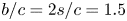 $b/c=2s/c=1.5$ and a rounded wing-tip geometry described by a semicircle centred at
  $(y',z')/c=(0,0.75)$ with a radius equal to the profile thickness at that
  $x'$ location (see figure 2).
Figure 2. A schematic of the wing-surface definition and its placement in the computational domain with the global Cartesian coordinate system  $(x,y,z)$ and its origin
  $O$ represented in black, the rotated wing coordinate system
  $(x',y',z')$ and its origin
  $O'$ represented in green, and the boundary layer coordinate system
  $(x_{BL},y_{BL},z_{BL})$ represented in red. Note that
  $(x_{BL},y_{BL},z_{BL})$ is shown at a random location on the wing for visual clarity, while its origin
  $O_{BL}$ is in fact on
  $O'$. The figure also shows the rounded (semicircle) wing-tip geometry and its definition. The wing has a chord length of
  $c$ and a semi-span of
  $s=b/2=0.75c$ (dark blue), with a geometric angle of attack of
  $\alpha$ (blue).
The wings are located such that their mid-chord,  $(x',y',z')/c=(0.5,0,0)$, coincides with the origin of the global Cartesian coordinate system,
  $(x,y,z)_O=(0,0,0)$, and have a no-slip, no-penetration boundary condition. The computational domain has a rectangular cross-section in the
  $z$-normal plane that extends
  $20c$ upstream,
  $30c$ downstream and
  $20c$ in positive and negative
  $y$ directions. Different angles of attack are achieved by rotating the wing along the
  $z$ axis around its centre
  $(x',y')/c=(0.5,0)$, located at
  $(x,y)=(0,0)$, without changing the inflow boundary condition. This specific design is to allow for the use of the ‘outflow-normal’ boundary condition (cf. Deville et al. Reference Deville, Fischer and Mund2002) on
  $y$-normal boundaries, which allows for a non-zero
  $y$ component of velocity (inward at
  $y=20c$ and outward at
  $y=-20c$ in lift-generating configurations). The inflow boundary at
  $x=-20c$ has a Dirichlet boundary condition with
  $(u_1,u_2,u_3)=(U_\infty,0,0)=\boldsymbol {U}_\infty$, while the outlet boundary at
  $x=30c$ has the outflow boundary condition. In order to avoid backflow at the outlet there is a sponge region for all
  $x \geq 10c$ with a gradually increasing forcing term that acts to bring the velocity to its free-stream condition. The effect of the sponge region on the flow has been tested in a number of preliminary runs and deemed negligible for all quantities of interest here.
The finite-span wing domain extends  $20c$ in the spanwise direction
  $z$ from the wing root (located at
  $z=0$) and has an ‘outflow-normal’ boundary condition at
  $z=20c$. A symmetry boundary condition is used at the
  $z=0$ plane (i.e. the wing root). While the symmetry condition forces the
  $z$ component of the velocity to be zero at the wing root (and thus, for instance, the corresponding Reynolds stress components), the impact of this boundary condition on turbulence quantities appears to be negligible for
  $z/c \geq 0.05$; therefore, simulation of full-span wings was not deemed necessary. The infinite-span (periodic) wings share the same domain design and boundary conditions in the
  $x$–
$x$– $y$ plane but have a spanwise width of
  $L_z=0.6c$ with periodic boundary conditions in
  $z$. The wider
  $L_z$ in these simulations (compared with previous works, e.g. Hosseini et al. Reference Hosseini, Vinuesa, Schlatter, Hanifi and Henningson2016; Negi et al. Reference Negi, Vinuesa, Hanifi, Schlatter and Henningson2018; Vinuesa et al. Reference Vinuesa, Negi, Atzori, Hanifi, Henningson and Schlatter2018) is to allow for a more accurate simulation of the wake region (not discussed here).
The boundary layers are tripped on both the suction and pressure sides in all seven cases. The implemented trip is a randomised time-dependent wall-normal force proposed by Schlatter & Örlü (Reference Schlatter and Örlü2012) (also see Hosseini et al. Reference Hosseini, Vinuesa, Schlatter, Hanifi and Henningson2016) aimed at minimising the required development length and history effects from the trip. The finite-span wings are only tripped on the main section of the wing ( $z<0.75c$), and not on the wing-tip region. On the suction side, the tripping is always located at
  $x'=0.1c$ regardless of the angle of attack, while on the pressure side it is at
  $x'=0.1c$ for the
  $0^\circ$,
  $2^\circ$ and
  $5^\circ$ angles of attack and at
  $x'=0.25c$ for
  $\alpha =10^\circ$. This change in the tripping location on the pressure side of the periodic wing at
  $\alpha =10^\circ$ was necessary since the acceleration parameter
  $K=(\nu /U_e^2)\,{\rm d}U_e/{\rm d}\kern0.07em x$ (where
  $U_e$ is the velocity at the boundary layer edge) far exceeded the rule-of-thumb value of
  $(2.5\unicode{x2013}3)\times 10^{-6}$ for relaminarisation (Spalart Reference Spalart1986; Yuan & Piomelli Reference Yuan and Piomelli2015) and the added energy in the tripping region was dissipated before generating turbulence. While this relaminarisation was only present in the periodic case, an early decision was made to match the location of the trip for finite- and infinite-span wings at the same geometric angle of attack
  $\alpha$. As will be seen in § 4, this was not an optimal choice; however, since it did not have an impact on the quantities studied here and due to the excessive cost of the simulations, this was not modified later.
2.3. Computational grids
The production grids used in this study are generated by iteratively adapting (i.e. refining) an initial grid using the solution-based spectral error indicator introduced by Mavriplis (Reference Mavriplis1990) for turbulent flows. From a mathematical point of view, this error indicator is an approximation of the interpolation error in the numerically obtained velocity field compared with its estimated exact counterpart (in an  $L^2$-norm sense), computed by estimating the truncation and quadrature errors (Offermans et al. Reference Offermans, Peplinski, Marin and Schlatter2020; Tanarro et al. Reference Tanarro, Mallor, Offermans, Peplinski, Vinuesa and Schlatter2020). From a physical perspective, this error indicator estimates the sum of the small-scale and unresolved turbulent kinetic energy (Toosi & Larsson Reference Toosi and Larsson2017), and corresponds to the numerical, modelling (from the large-eddy simulation model) and projection errors (Toosi Reference Toosi2019).
The initial grid for the periodic cases is conformal and originally two-dimensional, which is then extruded (i.e. copied to an appropriate number of spanwise locations) to make sure that the spanwise homogeneity of the mesh is maintained. Different angles of attack share the same near-wing mesh (up to a few boundary layer thicknesses), which is rotated with the wing. The root of the finite-span wing shares a nearly identical mesh with the periodic counterpart.
The production grids are generated by iterative refinement of the initial grids, where at each iteration elements with the highest contribution to solution error, identified by the volume-weighted error indicator (cf. Lapenta Reference Lapenta2003; Park Reference Park2003; Toosi & Larsson Reference Toosi and Larsson2020), are selected for refinement. The convergence process is accelerated by some manual input from the user; for instance, by manually marking the wall elements for refinement. The initial grids are designed to reach their desired wall resolution after four refinements of the near-wall elements. The automatic refinement is continued for a few iterations (where in the first four the wall elements are manually marked for refinement), and the refinement regions are then manually extended for three more iterations (i.e. each element is refined if any of its neighbouring elements is refined). This last step helps to avoid repeating the refinement process further (a process which becomes expensive for these progressively finer grids) and leads to a smoother and more uniform mesh. The adaptation process is terminated after reaching the resolution criteria from literature (such as those used in Vinuesa et al. (Reference Vinuesa, Hosseini, Hanifi, Henningson and Schlatter2017b, Reference Vinuesa, Negi, Atzori, Hanifi, Henningson and Schlatter2018)), expressed in terms of the viscous length scale  $\delta _\nu =\nu \sqrt {\rho /\tau _w}$ (where
  $\tau _w$ is the wall shear stress) for the boundary layer mesh, and the Kolmogorov length scale
  $\eta =(\nu ^3/\epsilon )^{1/4}$ (where
  $\epsilon$ is the local isotropic dissipation rate) for the wake region (cf. Pope Reference Pope2000).
Table 1 summarises some of the characteristics of the production grids used in this work. Note that the finite-span wings require significantly larger numbers of grid points compared with the periodic cases. This is partly to resolve the tip region and the larger span of these wings, and partly because of the decision to perform these simulations at slightly higher resolutions due to the potential insufficiency of the resolution criteria originally verified for canonical flows. For similar reasons, wings at higher angles of attack require higher numbers of grid points to accurately resolve all the important features of their more complex flow field with stronger vortices and secondary flows.
Table 1. Description of the production grids used in this study. The naming convention distinguishes the different set-ups by P- $\alpha$ for periodic wings at an angle of attack of
  $\alpha$ and RWT-
 $\alpha$ for finite-span wings at
  $\alpha ^\circ$ angle of attack. Here
  $N_{GLL}$ is the total number of GLL points (the number of independent grid points is around
  $0.67 N_{GLL}$). All values of
  $\Delta$ are based on the mean resolution computed as the element size divided by the polynomial order, whereas
  $\delta _1 y_{BL}$ is the distance from the wall of the first GLL point off the wall. Wall resolutions, including both
  $\Delta \ast _{BL}$ and
  $\Delta \ast _{tip}$, are reported along the wall coordinates
  $(x_{BL},y_{BL},z_{BL})$ (figure 2). The boundary layer resolutions
  $\Delta \ast _{BL}$ are normalised by the viscous length
  $\delta _\nu$ and reported at
  $(x',z')/c=(0.7,0.3)$ for the element on the wall. Tip resolutions
  $\Delta \ast _{tip}$ are normalised by the chord
  $c$ and reported at
  $x'/c=0.7$ and
  $z'=z'_{\rm max}$. Wake resolutions
  $\Delta \ast _{wake}$ are reported at
  $(x,z)/c=(2,0.3)$ at the location of minimum mean velocity.

Figure 3 shows the spectral elements of the RWT-10 grid, as a representative example of the grids used in this study, with instantaneous vortical structures of the flow visualised using the  $\lambda _2$ vortex identification method (Jeong & Hussain Reference Jeong and Hussain1995) added for visual reference.
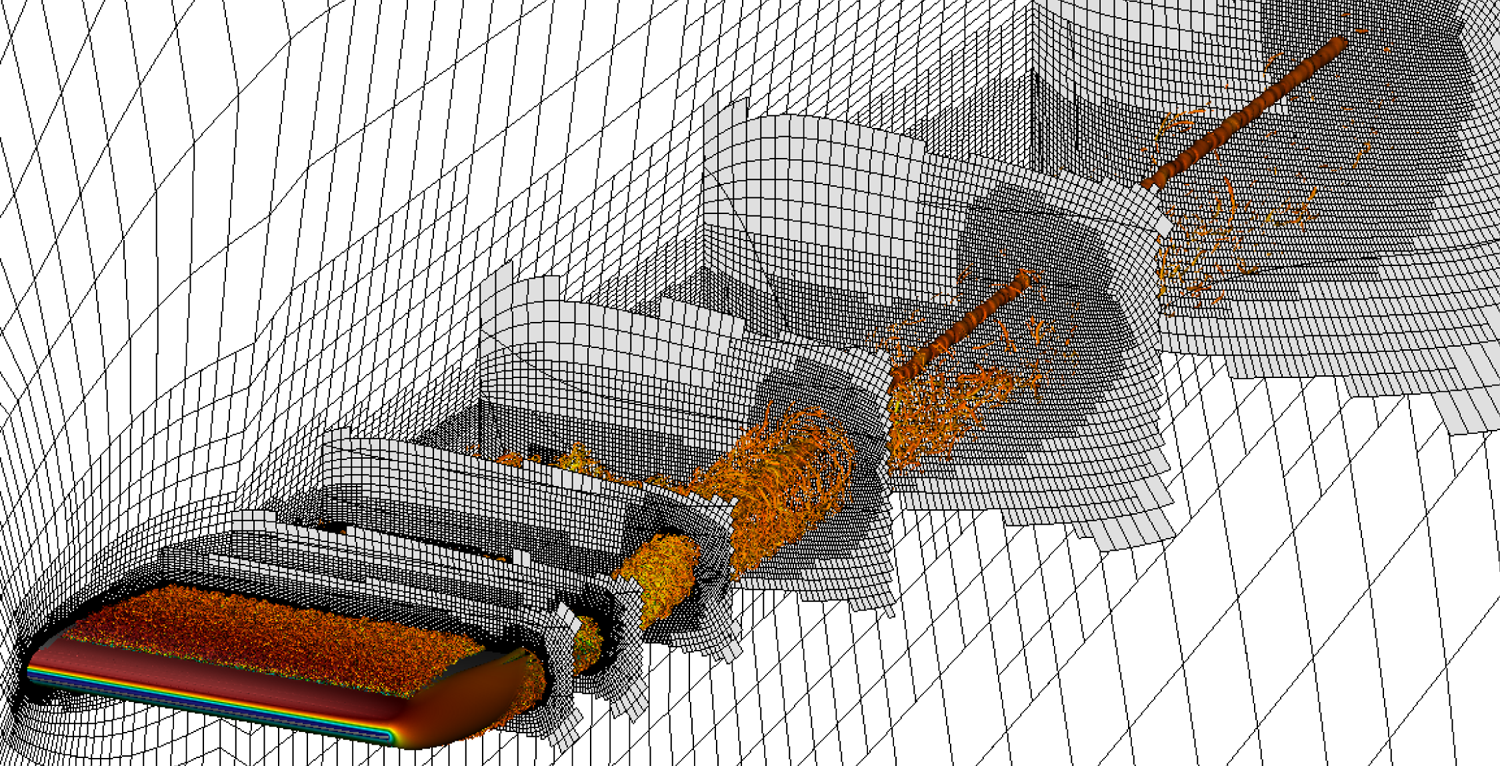
Figure 3. An example of the grids used in this study. Edges of the spectral elements of RWT-10 (with 4.23 million spectral elements; see table 1) are shown by black lines on a number of planar slices. The grid is generated using the  $h$-adaptation capabilities of the AMR version of Nek5000. The figure also shows instantaneous vortical structures represented by isosurfaces of
  $\lambda _2 c^2/U_\infty ^2=-100$ coloured by streamwise velocity ranging from low (blue) to high (red) for visual reference.
2.4. Flow transients and statistical averaging
Flow transients are removed both during the grid-adaptation stage and after reaching the production grid. In total, a minimum of approximately  $80c/U_\infty$ (equivalent to 80 convective time units,
  ${\mathcal {T}}_{conv}=c/U_\infty$) of integration time is discarded as transients. This comprises
  $50{\mathcal {T}}_{conv}$ on the coarse initial grid, roughly
  $25{\mathcal {T}}_{conv}$ on various adapted grids before reaching the production grid and an additional
  $4{\mathcal {T}}_{conv}$ on the production grid.
After the transient period, turbulence statistics are collected over a period of  $5{\mathcal {T}}_{conv}$ or above in the periodic cases (P-0, P-2, P-5, P-10), around
  $8 {\mathcal {T}}_{conv}$ for RWT-0, around
  $14 {\mathcal {T}}_{conv}$ for RWT-10 and for a longer period of around
  $23 {\mathcal {T}}_{conv}$ for RWT-5. Table 2 summarises the averaging time
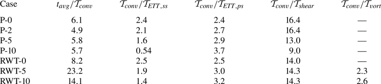
  $t_{\rm avg}$ used in each simulation in terms of the convective time unit. A conversion ratio is provided to relate
  ${\mathcal {T}}_{conv}$ to other time scales of the flow, including: the boundary layer eddy-turnover time
  ${\mathcal {T}}_{ETT}=\delta _{99}/u_\tau$, where
  $\delta _{99}$ is the
  $99\,\%$ boundary layer thickness and
  $u_\tau =\sqrt {\tau _w/\rho }$ is the friction velocity; the shear-layer (wake) time scale
  ${\mathcal {T}}_{shear}=\delta _{0.5, shear}/U_\infty$, where
  $\delta _{0.5, shear}$ is a measure of the wake thickness (see Pope Reference Pope2000); and the vortex-rotation time scale
  ${\mathcal {T}}_{vort}={\rm \pi} d_{vort}/u_{\theta,max}$, where
  $u_{\theta,{\rm max}}$ is the maximum azimuthal velocity around the vortex core and
  $d_{vort}$ is the vortex diameter measured as the distance between the two peaks in the azimuthal velocity around the core. Cases RWT-0 (which is symmetric around the
  $y=0$ plane and can be averaged in that direction) and RWT-5 have similar effective values of
  $t_{avg}/{\mathcal {T}}_{ETT,ss}$ (which is the most relevant time scale for the quantities studied here), while RWT-10 has a shorter integration time due to computational cost constraints.
Table 2. A summary of the averaging time  $t_{avg}$ used in each case compared with different time scales in the flow. Here
  ${\mathcal {T}}_{conv}$ is the convective (flow-over) time scale,
  ${\mathcal {T}}_{ETT}$ is the boundary layer eddy turnover time reported at
  $(x',z')/c=(0.7,0.3)$,
  ${\mathcal {T}}_{shear}$ is the shear time scale in the wake reported at
  $(x,z)/c=(2.0,0.3)$ and
  ${\mathcal {T}}_{vort}$ is the time scale of vortex rotation reported at
  $x/c=2.0$. Subscripts ‘
 $ss$’ and ‘
 $ps$’ stand for the suction side and pressure side of the wing. Definition of time scales is given in the text.
The statistics are collected on the fly (see Appendix A for more details) at a sampling rate that is around an order of magnitude higher than the highest frequency of the flow, here dictated by the viscous time scale  $\nu /u_\tau ^2$ (
 ${\geq } 2 \times 10^{-3} {\mathcal {T}}_{conv}$ for cases studied here). The periodic cases are homogeneous in the spanwise direction and therefore an ensemble average in that direction is also performed when computing the statistics. While RWT-0, RWT-5 and RWT-10 are fully 3-D flows and exhibit a variation of solution statistics along the span, these variations are smooth over the turbulent boundary layer section of the wings. This allows for a spanwise filtering of the statistics using a (wide) Gaussian filter with a variable filter width that is adjusted based on flow physics and resembles an averaging process. This procedure is explained in more detail in Appendix A.
The temporally and spatially averaged (or filtered) fields are denoted by  $\langle \cdot \rangle$; e.g.
  $\langle u_i \rangle$ and
  $\langle p \rangle$ for the mean velocity and mean pressure fields. The fluctuating part is then defined as the (point-wise) difference between the instantaneous and mean values; e.g.
  $u_i'=u_i-\langle u_i \rangle$ and
  $p'=p-\langle p \rangle$ for the fluctuating velocity and pressure fields.
In each case, the full statistical record is divided into four or more batches of equal size, which are used to estimate the uncertainty in solution statistics by computing the confidence intervals of each quantity of interest using the non-overlapping batch method (cf. Conway Reference Conway1963). Given the higher sensitivity of the Reynolds stresses, particularly for finite-span wings, their approximate error bars are included in the comparisons in § 4.3 and Appendix C. With the use of ensemble averaging along the span in periodic cases and the equivalent filtering in the wing-tip cases, the averaging times used in this work are deemed sufficient for the discussions here.
3. Flow around the finite-span wings
This section describes the important features of the flow around the finite-span wings of this study relevant to the discussions in § 4 and, to a certain degree, serves as an introduction to that section.
3.1. The instantaneous flow field
The flow around RWT-0, RWT-5 and RWT-10 is illustrated in figure 4 by the instantaneous vortical structures of the flow using the  $\lambda _2$ visualisation method of Jeong & Hussain (Reference Jeong and Hussain1995). The figure visualises the turbulent boundary layers formed on the wings, the turbulent wake and the wing-tip vortex identified as a cylindrical structure (surrounded by turbulent structures) that separates from the wing somewhere close to the tip and remains coherent for a long distance downstream of the wing (the entire field of view in figure 4). Note that the wing-tip vortex is only present in lift-generating configurations and absent in RWT-0. As expected, RWT-10 has a stronger wing-tip vortex (leading to a larger vortex diameter for a fixed value of
  $\lambda _2$) which impacts a larger portion of the wing, and more strongly, compared with RWT-5. While not directly relevant to the discussions of § 4, it is interesting to note that the vortex core in RWT-10 has a higher streamwise velocity compared with RWT-5, which is associated in the literature with the lower core pressure of the stronger wing-tip vortex and thus flow entrainment into the core region (cf. Lee & Pereira Reference Lee and Pereira2010).
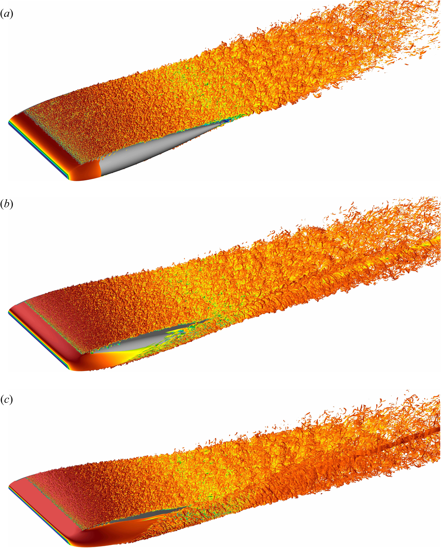
Figure 4. An overview of the flow around the finite-span wings: (a) RWT-0, (b) RWT-5 and (c) RWT-10. Plots show the instantaneous vortical structures, visualised by iso-surfaces of  $\lambda _2 c^2/U_\infty ^2=-100$ coloured by
  $u_1/U_\infty$ from
  $-$0.3 (blue) to 1.3 (red). The wing surface is shown in light grey.
The location of tripping and its effectiveness is visually clear in figure 4 by the absence of turbulent structures upstream of the trip and the presence of hairpin vortices (which the trip introduces through wall-normal forcing) downstream of the tripping line. The relatively low friction Reynolds number of the flow ( $200 \lesssim Re_\tau \lesssim 300$; see tables 3–5 in Appendix C) is apparent from the hairpin-dominated structure of the turbulent boundary layers (cf. Eitel-Amor et al. Reference Eitel-Amor, Örlü, Schlatter and Flores2015). Note that on both the suction and pressure sides the tripping line extends throughout the span of the wing from the root to the tip, but does not include the wing-tip region (the semicircle shown in figure 2). This results in a laminar flow around the wing tip and a laminar–turbulent interface at the spanwise end of the tripping line.
The figure shows a strong flow convection from the pressure side to the suction side (visualised by the convected turbulent structures from the pressure side), starting from the leading edge of the wing. This underscores the global impact of the finite span of the wing and the wing-tip vortices on the entire flow field. Case RWT-10 generates a higher lift and thus has stronger pressure gradients, leading to a stronger flow convection, stronger wing-tip vortices and stronger three-dimensionality in the flow field.
It is also important to note the appearance of a non-turbulent area on the suction side of RWT-5 and RWT-10 in a region close to the wing-tip vortex. This might initially suggest a relaminarisation of the turbulent boundary layer due to the increased pressure gradient, rotation and flow acceleration in the vicinity of the wing-tip vortex. However, upon further investigation this was proved not to be the case, since the turbulent region of the boundary layer was almost exactly following the streamlines of the flow released at the edge of the boundary layer near the spanwise end of the tripping line. In other words, the appearance of this laminar region should be primarily attributed to the non-zero spanwise velocity towards the root that convects the spanwise laminar–turbulent interface of the boundary layer in that direction and causes a laminar region to appear near the wing-tip region. Nevertheless, the present behaviour does not mean that extending the tripping line to include the tip region will necessarily lead to a fully turbulent suction side, since the strong flow acceleration, rotation and pressure gradients might still be sufficiently high to result in relaminarisation.
3.2. Mean-flow streamlines
The extent of three-dimensionality of the flow and its impact on the boundary layers are shown in figure 5 using the streamlines obtained from the mean velocity field  $\langle u_i \rangle$. The large deflection angle of the streamlines can be easily observed by comparison with the approaching free-stream direction (chord-wise lines). As expected, this deflection increases for all cases closer to the tip. Note that the deflection from the free-stream direction starts at the beginning of the boundary layer development and spans across a large region of the wing (almost the entire semi-span for these low-aspect-ratio wings). An interesting observation is that the streamlines of RWT-0 (which does not have a wing-tip vortex) are still impacted by the finite span of the wing and deflected towards the root, albeit with a lower deflection angle compared with RWT-5 and RWT-10. This is the reason for the appearance of a small laminar region close to the trailing edge of RWT-0 in figure 4(a). The other interesting observation is the large spanwise extent of the impacted boundary layer streamlines on the pressure side of RWT-5 and RWT-10 which is comparable to that on their suction side. On both the suction and pressure sides, the deflection angle approaches zero at the root of the wing as a result of the symmetry.

Figure 5. Contour plots of the pressure coefficient  $c_p$ on the wing surface for (a,d) RWT-0, (b,e) RWT-5 and (c, f) RWT-10 on the suction side (a–c) and pressure side (d–f) of the wings. Contour plots are overlaid with streamlines released at
  $x'/c=0.12$ at different
  $z'/c$ locations (0.1, 0.26, 0.43, 0.59, 0.75). The contour levels are from
  $-$1 (dark blue) to 1 (dark red) in increments of 0.1. The dotted black lines on the wing surface show the chord-wise direction (i.e. constant
  $z'$, equivalent to the approaching free-stream direction) at the same spanwise locations as the streamlines are released as a visual reference for their deflection. Arrows indicate the approximate direction of the free-stream velocity
  $\boldsymbol{U}_\infty$.
The more interesting observation from figure 5 is that the deflection angle of streamlines varies in the wall-normal direction across the boundary layer thickness  $\delta _{99}$. The streamlines closer to the wall have a larger deflection angle compared with those farther from the wall, and this is true on both the suction and pressure sides and at all spanwise locations. This is a common feature observed in many 3-D boundary layers (cf. Johnston Reference Johnston1960; Perry & Joubert Reference Perry and Joubert1965; Pierce et al. Reference Pierce, McAllister and Tennant1983; Ölçmen & Simpson Reference Ölçmen and Simpson1995; Devenport & Lowe Reference Devenport and Lowe2022) which happens due to the lateral pressure gradient encountered by the boundary layer and the variable balance between the different terms of the momentum equation, such that the fluid closer to the wall (which has a lower momentum) responds faster to the pressure gradient (cf. Devenport & Lowe (Reference Devenport and Lowe2022) and references therein). The variable deflection angle of the streamlines in the streamwise, wall-normal and spanwise directions has a number of consequences on the boundary layers, which is discussed further in § 4.
The wing-tip vortices are visible in RWT-5 and RWT-10 in figure 5(b,c) as streamlines that are clustered together and formed into spirals on the suction side of the wings. Additional details about the flow in the vicinity of the tip can be found in Appendix B. The generated wing-tip vortex impacts the surrounding flow differently depending on the distance. This is primarily related to the velocity induced by the vortex (the Biot–Savart law), which is proportional to the inverse of the distance from the vortex core (refer to the caption of figure 1) and approximately in the azimuthal direction of a cylindrical coordinate system with the vortex core at its origin. Due to the large variations in both magnitude and direction of the induced velocity, the flow in the vicinity of the vortex core is highly non-homogeneous. The flow acceleration due to pressure gradient is also larger near the tip. At larger spanwise distances from the vortex – and farther downstream from the location of its initial formation – the induced velocity on the wing surface becomes a nearly unidirectional downwash with a variable magnitude (and, thus, a variable effective angle of attack along the span). We take advantage of this behaviour of finite-span wings to facilitate the analyses in § 4.
Figure 5 also shows the contour lines of the pressure coefficient  $c_p=2(p-p_\infty )/\rho U_\infty ^2$ on the surface of the wings. Note that the wall-parallel component of pressure gradient (at the wall and across the boundary layer thickness) is orthogonal to the constant
  $c_p$ lines represented in the figure. An increasing trend in the pressure coefficient (and therefore pressure) can be observed approaching the tip region. This pressure gradient is the main cause for the observed streamline deflections in RWT-0. The boundary layer streamlines on the suction side of RWT-5 and RWT-10 are deflected towards the root as a result of these pressure gradients and the high momentum of the flow approaching the suction side from the pressure side. There is also a pressure gradient on the pressure sides of RWT-5 and RWT-10, albeit weaker, which causes the flow to accelerate towards the tip of the wing. On both sides, the pressure gradient decreases in magnitude and becomes more aligned with the streamlines closer to the wing root (characterised by contour level lines that are more aligned with the spanwise direction and farther apart from each other). This implies that the fluid particles following the streamlines are subjected to reduced accelerations due to pressure gradient. Consequently, the streamlines approximate straighter lines, leading to less variation in the deflection along a given streamline. This in turn mitigates some of the 3-D effects that result from the skewed velocity profile.
4. Turbulent boundary layers
The finite span of the wings and the induced three-dimensionality by the wing-tip vortices have a number of important impacts on the boundary layers developing on RWT-0, RWT-5 and RWT-10. The goal of this section is to separate and simplify these effects as much as possible in §§ 4.1 and 4.2, before analysing the remaining finite-span effects more closely in § 4.3.
4.1. The impact of the effective angle of attack
Figure 6 plots the  $99\,\%$ boundary layer thickness
  $\delta _{99}$ defined based on the diagnostic scaling (Vinuesa et al. Reference Vinuesa, Bobke, Örlü and Schlatter2016) and the Clauser pressure-gradient parameter
  $\beta _{x_{BL}}$ (Clauser Reference Clauser1954, Reference Clauser1956), at a spanwise location near the root. The Clauser parameter is computed along
  $x_{BL}$ (defined in figure 2) as
 \begin{equation} \beta_{x_{BL}} = \frac{\delta^*}{\vert \tau_{w} \vert} \frac{\partial P_e}{\partial x_{BL}} , \end{equation}
where  $\delta ^*$ is the boundary layer displacement thickness,
  $\vert \tau _{w} \vert$ is the shear-stress magnitude at the wall and
  $P_e=\langle p(x_{BL},\delta _{99},z_{BL}) \rangle$ is the pressure at the edge of the boundary layer.

Figure 6. The  $99\,\%$ boundary layer thickness
  $\delta _{99}$ (a,b) and the Clauser pressure-gradient parameter
  $\beta _{x_{BL}}$ (c,d) plotted at
  $z'/c=0.1$ (close to the root) on the suction side (a,c) and pressure side (b,d) of the wings of this study. The finite-span wings are plotted in solid lines, while periodic airfoils are shown by the dotted lines. Colours, from light to dark, correspond to angles of attack of
  $\alpha =0^\circ$,
  $2^\circ$,
  $5^\circ$ and
  $10^\circ$, respectively, for infinite-span wings. The three finite-span wings are shown with matched colours to the infinite-span ones at the same
  $\alpha$. The observed differences are mainly attributed to the impact of the reduced effective angle of attack
  $\alpha _{eff}$ (an inviscid effect caused by the induced downwash of the wing-tip vortex; see figure 1) on the boundary layers.
There is a large difference between the boundary layers formed on the finite-span wings compared with the periodic ones at the same angle of attack. Namely, the boundary layers on the suction sides are thinner and encounter lower adverse pressure gradients (lower  $\beta _{x_{BL}}$ values), while they are thicker on the pressure side and encounter a larger Clauser parameter (interesting to note that
  $\beta _{x_{BL}}>0$ over the majority of the pressure side as well). Furthermore, the discrepancies are larger for higher angles of attack and nearly vanish for
  $\alpha =0^\circ$. These are all consequences of the lower effective angle of attack
  $\alpha _{eff}$ of the finite-span wings compared with their geometric angle of attack
  $\alpha$ (a well-known inviscid effect caused by the induced downwash of the wing-tip vortex, explained in figure 1). This is further demonstrated by figure 7 which shows the section-wise pressure component of the lift and drag coefficients of all cases defined as
 $$\begin{gather} c_{L,p}(z_0) = \frac{2}{\rho U_\infty^2 c} \oint {(\langle p(x_{BL},0,z_0) \rangle \boldsymbol{\cdot} \boldsymbol{e}_{n})\, {\rm d}\kern0.07em{x}_{BL}}, \end{gather}$$
 $$\begin{gather}c_{D,p}(z_0) = \frac{2}{\rho U_\infty^2 c} \oint {(\langle p(x_{BL},0,z_0) \rangle \boldsymbol{\cdot} \boldsymbol{e}_{t}) \,{\rm d}\kern0.07em{x}_{BL}}, \end{gather}$$
where  $\boldsymbol {e}_{n}$ is a unit vector normal to the wall and opposite to
  $y_{BL}$,
  $\boldsymbol {e}_{t}$ is a unit vector tangential to the wall in the same direction as
  $x_{BL}$ and
  $\rho$ and
  $c$ are the fluid density and chord length. The integrals are taken on the wing surface (
 $y_{BL}=0$) over both the suction and pressure sides at a fixed spanwise location
  $z_{BL}=z_0$. Assuming a linear variation of the lift coefficient with angle of attack in infinite-span wings (which is approximately true for relatively low angles of attack; cf. Houghton et al. Reference Houghton, Carpenter, Collicott and Valentine2013; Federal Aviation Administration 2016) we could make the approximation that
 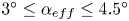 $3^\circ \leq \alpha _{eff} \leq 4.5^\circ$ for RWT-10 (with it being closer to
  $4.5^\circ$ at the root and around
  $3^\circ$ close to the tip) and
  $1^\circ \leq \alpha _{eff} \leq 2^\circ$ for RWT-5 (the lifting-line theory (cf. Houghton et al. Reference Houghton, Carpenter, Collicott and Valentine2013) leads to similar approximated values for
  $\alpha _{eff}$ over the majority of the span). This justifies the fact that in figure 6 both the boundary layer thickness and the Clauser parameter on the suction side of RWT-10 are very close to those of P-5, or why the RWT-5 curves (corresponding to
  $\alpha _{eff} \approx 2^\circ$ at the root) are closer to P-2.

Figure 7. The section-wise (a) pressure lift and (b) pressure drag coefficients along the span for all the geometries of this study. Line styles and colours are the same as those in figure 6. The additional thin solid lines in (a) are from inviscid simulations of finite-span wings for the same configurations as RWT-0, RWT-5 and RWT-10. The nearly identical variation of pressure lift coefficient (approximately proportional to  $\alpha _{eff}$) emphasises the inviscid nature of the phenomenon. Refer to figure 1(b) and its caption for a schematic explanation of the induced drag which explains the increased drag coefficient of the finite-span wings.
It is important to emphasise that the observed similarity based on effective angles of attack is in fact a result of an approximate similarity of the pressure gradient and boundary layer histories. Therefore, our reliance on  $\alpha _{eff}$ in the next sections is meant as an approximate equivalence of pressure gradients and history effects. In fact, there are additional (inviscid) effects caused by a positive (i.e. away from the wall) and variable wall-normal velocity along the span, especially near the tip at locations earlier in the development of the wing-tip vortex, that are not captured by the simplified use of
  $\alpha _{eff}$. These effects are discussed further in § 4.3.
Figure 7(a) also compares the turbulent finite-span wings, RWT-0, RWT-5 and RWT-10, with inviscid (incompressible Euler) simulations of the same set-ups (without the tripping) performed using the open-source solver SU2 (Economon et al. Reference Economon, Palacios, Copeland, Lukaczyk and Alonso2016). The nearly identical variation of the lift (and effective angle of attack) over a large portion of the span emphasises the inviscid nature of the phenomenon. The larger observed differences near the tip should be mainly attributed to the difference in vortex formation and the resulting change in both the vertical and spanwise location of the vortex in inviscid flows. These differences are discussed briefly in Appendix B. Additional viscous effects are present near the tip and are expected to contribute to the observed differences in that region; however, they are not discussed here.
4.2. Collateral flow and transformation into wall-shear coordinates
The skewed velocity profile and the variable deflection angle of the streamlines (figure 5) result in additional non-zero velocity gradient components, and, consequently, the activation of additional production terms in the transport equations of  $\tilde {{\mathsf{R}}}_{13}$,
  $\tilde {{\mathsf{R}}}_{23}$ and
  $\tilde {{\mathsf{R}}}_{33}$ (for
  $\tilde {{\mathsf{R}}}_{ij}=\langle u'_i u'_j \rangle _{BL}$ denoting the Reynolds stress expressed in
  $(x_{BL},y_{BL},z_{BL})$ coordinates) with the largest impact on the production of
  $\tilde {{\mathsf{R}}}_{13}$.
The main goal of this section is to use the flow characteristics to find a coordinate system that simplifies the analysis.
Figure 8 plots the deflection angle  $\gamma _{stream}$ defined as the angle between the wall-parallel part of the velocity vector and the wall-parallel direction
  $x_{BL}$ (with the wall-normal component of the velocity vector
  $\langle u_2 \rangle _{BL}$ excluded). Visually, this is the angle that the streamlines of figure 5 make with the chord-wise lines (free-stream direction). While
  $\gamma _{stream}$ is highly variable across the boundary layer thickness, it exhibits an important quality: it is approximately constant in the most active and important region of wall turbulence,
  $y_{BL}^+ \leq 30$. This region of collateral flow is a common feature of many 3-D boundary layers (cf. Johnston Reference Johnston1960; Perry & Joubert Reference Perry and Joubert1965; Pierce et al. Reference Pierce, McAllister and Tennant1983; Ölçmen & Simpson Reference Ölçmen and Simpson1995; Devenport & Lowe Reference Devenport and Lowe2022). In the context of our discussion, this means that the most active part of the near-wall region can potentially be considered nearly two-dimensional in a rotated coordinate system that is aligned with the direction of the streamlines in the
  $y_{BL}^+ \leq 30$ region. The region above
  $30\delta _\nu$ still experiences a variable shear, but since both the Reynolds stresses and mean velocity gradients are significantly smaller in this region, the contribution from the new production terms (which are the product of the Reynolds stresses and the mean velocity gradient) will remain low for a large portion of the boundary layer.

Figure 8. The deflection angle (in degrees) at  $x'/c=0.7$ for multiple spanwise locations from
  $z'/c=0.1$ to 0.6 (with 0.02 increments) on the suction side (a–c) and the pressure side (d–f) of (a,d) RWT-0, (b,e) RWT-5 and (c, f) RWT-10. Darker colours are sampled closer to the tip. Circles show the edge of the boundary layer,
  $\delta _{99}$. Negative (positive)
  $\gamma _{stream}$ values correspond to deflection towards the root (tip). Note the relatively constant value of
  $\gamma _{stream}$ for
  $y_{BL}^+ \leq 30$.
In the rest of this paper the boundary layers are studied in a coordinate system  $(x_\tau,y_\tau,z_\tau )$, which is defined by rotating
  $(x_{BL},y_{BL},z_{BL})$ (figure 2) around its wall-normal axis
  $y_{BL}$ in such a way that
  $x_\tau$ becomes aligned with the direction of the wall-shear stress (the streamlines). Note that the orientation of this coordinate system changes across both the span and the chord of the wing (see the streamlines of figure 5). This does not affect the analysis in the rest of the paper which is performed in local coordinates.
The rotated Reynolds stress components exhibit a structure that is very close to that of a two-dimensional boundary layer, where  ${\mathsf{R}}_{13} \approx {\mathsf{R}}_{23} \approx 0$ (for
  ${\mathsf{R}}_{ij}=\langle u'_i u'_j \rangle _\tau$ denoting the Reynolds stress expressed in
  $(x_\tau,y_\tau,z_\tau )$ coordinates). This simplification is possible for these boundary layers mostly because of the relatively small change in the deflection angle across the boundary layer thickness (less than
  $10\,^\circ$; see figure 8) and is not necessarily possible for all 3-D boundary layers. The spanwise component of the mean velocity is by definition close to zero for
  $y_\tau ^+\leq 30$ in this coordinate system and only increases closer to the edge of the boundary layer. This results in a Reynolds stress production term close to that of a statistically two-dimensional boundary layer for similar conditions. The obtained simplification by rotation into the
  $(x_\tau,y_\tau,z_\tau )$ coordinate system cannot remove the less local effects. Such effects are discussed in the next section.
4.3. Additional departures from infinite-span wings
Two other notable effects are associated with the finite span of the wing and the 3-D flow field:
(i) Flow acceleration from the pressure side towards the suction side, during the formation of the wing-tip vortices, results in a wall-normal velocity that is different along the chord and the span of the wing. This variation is such that the locations closer to the tip and earlier in the development of the wing-tip vortex (i.e. closer to the leading edge) experience higher positive wall-normal velocities. The wall-normal velocity impacts the development of the boundary layers, such that increased values of this quantity lead to a faster growth rate. As a result, there is a slight increase in
 $\delta _{99}$ on the suction side for locations closer to the tip, and similarly thinner boundary layers closer to the tip on the pressure side. This is primarily an inviscid effect.
(ii) Variation of the deflection angle with normal distance from the wall (a result of variable momentum across
$y_\tau$, mainly due to viscous effects) means that streamlines crossing a wall-normal line have converged from different spanwise locations on the wing. Since the effective angle of attack, and thus the streamwise pressure gradients, are different at different spanwise locations (mostly an inviscid effect), fluid particles at different wall-normal locations have experienced different histories. This effect is larger closer to the tip region, where both the variation in the deflection angle (see figure 8) and the variation in the pressure gradient (approximately characterised by the effective angle of attack; see figure 7) are larger.


This section investigates and characterises these effects by comparing the boundary layers formed on the finite-span wings with their equivalent from the infinite-span wings. Equivalence is quantified here as closeness in terms of the local values of  $Re_\tau$ and
  $\beta _{x_\tau }$, as well as similarity of their history. Appendix C explains in more detail the procedure used to match each of these quantities. The importance of this procedure is discussed briefly at the end of this section.
Figure 9 depicts the variation of the normal streamwise Reynolds stress,  ${\mathsf{R}}_{11}=\langle u'_1 u'_1 \rangle _\tau$, in RWT-5 as a function of the streamwise and spanwise locations. Additional Reynolds stress components, additional locations and other angles of attack are included in figures 12–14 in Appendix C. Only a subset of those profiles that are representative of the overall trends and behaviours is shown here. We focus solely on the suction side of the wings, both here and in Appendix C. This choice is motivated by the higher Reynolds number and more interesting behaviour exhibited on the suction side. Information concerning the pressure side of the wings, as well as the suction side, including all turbulence statistics, is accessible in the simulation database (refer to the data availability statement).

Figure 9. Variation of the inner-scaled Reynolds stress  ${\mathsf{R}}_{11}^+$ with (a,b) streamwise distance from the leading edge and (c,d) spanwise distance from the root. The evolution along streamlines released at (a)
  $(x'_{start},z'_{start})/c=(0.12,0.1)$ and (b)
  $(x'_{start},z'_{start})/c=(0.12,0.72)$, and the intersection of four streamlines released at
  $x'_{start}/c=0.12$ at spanwise locations
  $z'_{start}/c=0.1$,
  $0.31$,
  $0.51$,
  $0.72$, with planes at (c)
  $x'/c=0.6$ and (d)
  $x'/c=0.9$. Profiles are shifted vertically by
  $2$ units with increasing
  $x'$ or
  $z'$ for visual clarity. The profiles are from RWT-5 (solid lines) and P-2 (dashed lines), and are a subset of those plotted in figure 13. All streamlines are released in the near-wall (approximately collateral) region. See text and Appendix C for more details. Shaded regions correspond to 80 % confidence intervals of the inner-scaled Reynolds stress profiles (due to finite time averaging), computed from the non-overlapping batch method (cf. Conway Reference Conway1963). Case P-2 has extremely narrow confidence intervals which are not plotted.
The initial pattern identified in figure 9(a,b) reveals an overall increase in  ${\mathsf{R}}_{11}^+={\mathsf{R}}_{11}/u_\tau ^2$ in the direction of development of the streamlines (i.e. increasing
  $x'$) and the emergence of a more active outer region. This is observed in both finite-span and infinite-span profiles and exhibits considerable similarity across both types. This phenomenon is attributed to the adverse pressure gradient effects, a topic extensively studied in the literature (cf. Spalart & Watmuff Reference Spalart and Watmuff1993; Perry et al. Reference Perry, Marusic and Jones2002; Aubertine & Eaton Reference Aubertine and Eaton2005; Monty et al. Reference Monty, Harun and Marusic2011; Harun et al. Reference Harun, Monty, Mathis and Marusic2013; Bobke et al. Reference Bobke, Vinuesa, Örlü and Schlatter2017; Bross et al. Reference Bross, Fuchs and Kahler2019; Devenport & Lowe Reference Devenport and Lowe2022; Pozuelo et al. Reference Pozuelo, Li, Schlatter and Vinuesa2022). Despite its significance, this phenomenon is not the primary focus of this study. Instead, our attention is devoted exclusively to exploring the differences between the finite- and infinite-span boundary layers.
Figure 9(b) demonstrates a reduction in the near-wall peak of  ${\mathsf{R}}_{11}^+$, which appears to magnify downstream. This discrepancy mainly arises due to the milder adverse pressure gradient experienced by the boundary layer closer to the tip. This is a consequence of the lower effective angle of attack in that region.
Another trend evident in figure 9(b) is the increased Reynolds stress level in the outer region of the boundary layer, particularly near its edge. This effect becomes more pronounced in spanwise locations closer to the tip (compare figure 9a,b), and it displays a growing spanwise influence as one moves downstream (compare figure 9c,d). This phenomenon can be attributed to the increased wall-normal velocity and its wall-normal gradient closer to the wing's tip. This is illustrated in figure 10(a) for two streamwise locations. The increased wall-normal velocity results in increased boundary layer growth (enhanced  $\partial \langle u_1 \rangle _\tau / \partial x_\tau$ due to the continuity equation) and an increased boundary layer thickness, manifesting as a non-zero Reynolds stress at greater distances from the wall. It is worth noting that the spanwise variation in wall-normal velocity diminishes as one moves downstream. Such observations suggest that the widening spanwise influence of this effect originates from the upstream state of the boundary layer, its flow development towards the root and propagation of non-zero fluctuations in the spanwise direction (due to mixing and transport).

Figure 10. The variation of wall-normal velocity along the span at two streamwise planes (a) and the variation of the outer-scaled  ${\mathsf{R}}_{11}$ in the streamwise direction (b). All solid lines correspond to RWT-5. Darker colours in (a) denote locations closer to the tip at the intersection of the same streamlines used in figure 9. Profiles shown in (b) are the same as plotted in figure 9(b), with dotted lines corresponding to matched
  $x'$ locations from P-2, and dashed lines corresponding to matched
  $Re_\tau$ and
  $\beta _{x_\tau }$ (simple dashed lines) and matched boundary layer thickness
  $\delta _{99}$ (dashed lines with triangles), both from P-2. Profiles are shifted vertically by
  $0.01$ units in (a) and
  $5\times 10^{-3}$ units in (b) for visual clarity. Shaded regions in (b) correspond to 80 % confidence intervals in the outer-scaled Reynolds stress profiles (due to finite time averaging), computed from the non-overlapping batch method. Panel (a) has narrow confidence intervals which are not plotted.
At these low Reynolds numbers, the development length available for the boundary layers, proportional to  $c/\delta _{99}$, is quite limited. This results in a transient response from the boundary layers to the change in their thickness, primarily characterised as a shift in the location of the outer structures away from the wall, which propagates throughout the boundary layer thickness as it develops. This hypothesis is examined in figure 10(b), where the profiles from figure 9(b) are shown in outer units. These profiles are contrasted in the figure with their infinite-span counterparts at matched
  $(Re_\tau, \beta _{x_\tau })$ and matched
  $\delta _{99}$. A shift in the location of the outer structures away from the wall would manifest itself as a coincident Reynolds stress profile near the boundary layer edge, which is indeed the observed behaviour in figure 10(b).
The wall-normal extent of agreement around the boundary layer edge decreases downstream. This phenomenon may be attributed to the development of the boundary layers and their gradual response to the changes induced by the increased boundary layer thickness. Further implications of this behaviour are discussed later.
The spanwise variation of  ${\mathsf{R}}_{11}^+$ is illustrated in figure 9(c,d). A trend of diminishing magnitude in the near-wall peak of the Reynolds stress is evident, particularly when approaching the tip. This phenomenon can be attributed to a few underlying mechanisms.
First, the effective angle of attack, which varies in the spanwise direction, diminishes closer to the tip. As a result, milder adverse pressure gradients occur near the tip (characterised by lower  $\beta _{x_\tau }$ values). This leads to a lower increase in the inner-scaled Reynolds stress profile and the turbulent kinetic energy due to adverse pressure gradients (in their development in the streamwise direction). Consequently, the overall inner-scaled Reynolds stress levels decrease, resulting in a diminished near-wall peak. In RWT-10 (see figure 14), there is a larger variation in
  $\alpha _{eff}$ and
  $\beta _{x_\tau }$ across the span compared with RWT-5, which can partially explain the steeper decline of the near-wall peak in RWT-10.
Closer to the tip, the increased deflection angle near the wall results in laminar flow entrainment into the turbulent boundary layers at their outmost spanwise extent. This entrainment is more pronounced in the collateral region  $y_{BL}^+\leq 30$ with the highest deflection angles. Consequently, diminished near-wall turbulence activity can be expected close to the spanwise edge of the turbulent boundary layers. Such reductions in turbulence can influence the near-wall peak of
  ${\mathsf{R}}_{11}^+$ outside areas directly subjected to flow entrainment. This could be another reason for the observed decline of the near-wall peak for locations plotted in figure 9. Further investigations are necessary to evaluate the significance of this mechanism in comparison with others.
The other mechanism that contributes to attenuation of the near-wall peak of  ${\mathsf{R}}_{11}^+$ is linked to the discussed increase in growth rate of the boundary layers near the tip. This, on the one hand, reduces the production term near the wall through decreased velocity gradients in the wall-normal direction, and, on the other, leads to additional transport away from the wall. Both of these mechanisms contribute towards reducing the peak in
  ${\mathsf{R}}_{11}^+$ profiles.
Another element to consider is the spanwise pressure gradient present within the boundary layers, quantified by  $\beta _{z_\tau }$ in tables 3–5. To take advantage of the findings of Lozano-Durán et al. (Reference Lozano-Durán, Giometto, Park and Moin2020), an equivalent expression for their parameter
  $\varPi$ can be established by considering the relation
  $\partial \langle p \rangle / \partial x=\tau _w/\delta$ in fully developed channel flows (where
  $\delta$ is the channel half-height). This leads to a definition of
  $\varPi$ in turbulent boundary layers as
 \begin{equation} \varPi \approx \frac{\delta_{99}}{\tau_w} \frac{\partial P_e}{\partial z_\tau} = \frac{\delta_{99}}{\delta^*}\beta_{z_\tau} . \end{equation}
This parameter was found to be always below  $0.015 Re_\tau$ at all locations reported here and in figures 12–14. This is well below the range of the approximate value of
  $\varPi > 0.03 Re_\tau$ suggested by Lozano-Durán et al. (Reference Lozano-Durán, Giometto, Park and Moin2020) as the regime in which the effect of spanwise pressure gradients becomes significant. As a result, it is unlikely for this mechanism to have a significant impact on the attenuation of turbulence and the near-wall peak of the Reynolds stress profile. It should be noted that the recommended criterion was derived for higher
  $Re_\tau$, in the absence of adverse pressure gradients, and for an initially fully developed channel flow. Whether a violation of these conditions leads to significant departures from the proposed criterion is not entirely clear and merits further investigation.
It is important to acknowledge certain observed departures in figures 12–14 from the trends described above. Firstly, RWT-0 exhibits a profile almost identical to P-0 near the root at  $x'/c=0.6$ (figure 12a), yet later evolves to display lower levels of fluctuations for
  $y_{BL}^+ \geq 30$ at downstream locations as early as
  $x'/c=0.7$, despite having the same boundary layer thickness. While this is most likely an artefact caused by differences in the trip or different response of the boundary layers to the trip (e.g. a history effect), further investigations are needed to ascertain whether this might be a consequence of additional unidentified mechanisms. Another noticeable departure is found in the case of RWT-10, particularly at
  $x'/c=0.8$ and
  $0.9$ (figure 14k,l,o, p), which do not display a decrease in the near-wall peak. Possible explanations for this behaviour could include the larger variation of
  $\beta _{x_\tau }$ at those locations, the reduced deflection angle at
  $x'/c=0.8$ and
  $0.9$ (see figure 5c) and the stronger 3-D effects in RWT-10.
Before concluding this section, we should emphasise that the reference profiles chosen for the comparisons in this section were specifically selected to eliminate as many causes of difference between the finite- and infinite-span profiles as possible. This ensures that the observed differences primarily arise from a few key mechanisms. However, this selection also results in smaller differences between the compared profiles, which may not be fully representative of the real discrepancy. This point is partially illustrated in figure 10(b), which shows a larger difference in  ${\mathsf{R}}_{11}$ profiles when only the streamwise locations are matched. It is worth noting that, at the spanwise location selected for this figure, RWT-5 exhibits a reduced effective angle of attack of approximately
  $1^\circ$. Given that a decreased effective angle of attack leads to thinner boundary layers and a higher outer-scaled near-wall peak in
  ${\mathsf{R}}_{11}$, the actual disparity between the finite- and infinite-span wings is likely greater than what is depicted in the figure.
5. Summary and conclusions
High-fidelity simulations of finite-span wings with a symmetric NACA0012 profile and a rounded wing-tip geometry were performed at a chord-based Reynolds number of 200 000 in free-flight conditions. Three angles of attack ( $0^\circ$,
  $5^\circ$ and
  $10^\circ$) were considered and supplemented with infinite-span (periodic) wings at corresponding geometric and effective angles of attack. Tripping was used to ensure turbulent boundary layers on both the suction and pressure sides. The resulting database can be used for a number of academic and engineering applications, including careful studies of the boundary layers and the wake, the wing-tip vortex and its formation, development and interaction with the surrounding flow or improving the turbulence models such as the Reynolds-averaged Navier–Stokes models or wall models used in large-eddy simulations. The main focus here was on the effect of wing-tip vortices and their induced three-dimensionality on the turbulent boundary layers. Other aspects of the flow will be studied in future works.
The general flow field of the lift-generating wings (RWT-5 and RWT-10) was characterised by the presence of a main wing-tip vortex as well as additional secondary vortices formed on the suction side of the wings. These vortices were stronger and formed earlier for higher angles of attack. A spanwise pressure gradient was present in all finite-span cases (a well-known inviscid effect), including RWT-0 which does not generate lift. As a result of this pressure gradient the boundary layers were deflected towards the root on the suction side and towards the tip on the pressure side. The deflection angle was different across the span and chord of the wing, but also in the wall-normal direction due to the faster response of the low-momentum fluid near the wall (see Devenport & Lowe (Reference Devenport and Lowe2022) and references therein).
Despite the non-canonical nature of these boundary layers, they could be simplified by first accounting for the effective angle of attack and its impact on the pressure gradient imposed on the boundary layers, followed by a (tensor) rotation into a coordinate system aligned with the direction of wall shear. This could further simplify the structure of the Reynolds stress tensor and make it similar to a two-dimensional boundary layer, where  ${\mathsf{R}}_{13} \approx {\mathsf{R}}_{23} \approx 0$. Two additional effects were observed and discussed. Firstly, the variable deflection angle across the boundary layer thickness means that the fluid particles across a wall-normal line have converged from different spanwise locations, and due to the variable pressure gradient across the span have different histories. Secondly, the variable wall-normal velocity along the span, with higher values closer to the tip, leads to a higher growth rate for the boundary layer farther from the root. Each of these mechanisms has additional consequences. The normal streamwise Reynolds stress
  ${\mathsf{R}}_{11}$ (as well as the other components) of the finite-span boundary layers was compared with the corresponding profiles from infinite-span wings, the observed differences were explained and the mechanisms at play were discussed. Some of these differences could not be fully explained by the simplified representation here and thus need further investigations.
Different terms in the transport equation of the turbulent kinetic energy and Reynolds stresses (i.e. the budget terms; see Pope Reference Pope2000) were computed (and are available in the simulation database; see the data availability statement), but were not shown or discussed here. This was because no additional insight was gained from those terms. For example, while a decrease in the production of  ${\mathsf{R}}_{11}$ was observed near the wall, this was as much a consequence of the decreased near-wall peak of
  ${\mathsf{R}}_{11}$ as it was a cause. Similarly, the increase in the production term near the boundary layer edge and a corresponding increase in the dissipation term could be attributed to the increased
  ${\mathsf{R}}_{11}$ in that region and the required balance between different terms. This highlights the need for predictive models in wall turbulence.
It is important to emphasise that the assumptions leading to § 4.3, and the subsequent conclusions, are not valid close to the wing-tip vortex or the trailing edge of the wing. For instance, for spanwise locations slightly closer to the tip than those discussed here, while still inside the turbulent region of the boundary layer, the near-wall streamlines have entered from the laminar flow region near the vortex. At the trailing edge, the boundary layer on the suction side with a spanwise velocity towards the root (i.e.  $\langle u_3 \rangle <0$) approaches the boundary layer on the pressure side with its spanwise velocity towards the tip (
 $\langle u_3 \rangle >0$). The two boundary layers also have opposite wall-normal and different streamwise velocities. These complex trailing-edge effects were not discussed here.
Throughout this work we relied on quantities such as the Clauser pressure-gradient parameter, with little modification in their formulation or discussion about their application in complex or 3-D boundary layers. Here, the 3-D effects were somewhat weak and we mostly relied on qualitative comparisons; therefore, the current definitions were deemed sufficient. Going forward, careful studies of the role and optimal definition of such parameters in 3-D boundary layers, and potentially developing new ones, are absolutely essential.
Many of the attributes of 3-D turbulent boundary layers (summarised in Devenport & Lowe (Reference Devenport and Lowe2022)) were not observed here. This includes effects such as depressed wake of the mean velocity profile (cf. Spalart, Coleman & Johnstone Reference Spalart, Coleman and Johnstone2008), reduction in the Townsend structure parameter (cf. Littell & Eaton Reference Littell and Eaton1994) or a significant change in the pressure–strain term (cf. Lozano-Durán et al. Reference Lozano-Durán, Giometto, Park and Moin2020). This is most likely due to the relatively weak variation of the deflection angle in the wall-normal direction, and the gradual variation of this and other similar parameters along the streamlines, both of which allow the boundary layers to recover (or approach) their two-dimensional state. In terms of modelling, the weak three-dimensionality of these boundary layers makes it easier to adapt the current turbulence models to account for these effects.
The wings of this study had a relatively low aspect ratio of 1.5. This was a deliberate choice, motivated by the scope of this study, the stronger 3-D effects near the tip and as a measure to save cost. For a fixed Reynolds number, a wing with a higher aspect ratio will experience a higher effective angle of attack and a stronger vortex. It will also have a slightly different spanwise variation in its effective angle of attack due to the change in the spanwise distance to the mirror vortex. A potentially more significant impact of the low aspect ratio is the (global) blocking effect of the symmetry plane on the spanwise velocity, which could lead to higher variations in the deflection angle along the span or a slightly different location of the wing-tip vortex. While it is important to keep these in mind when generalising the findings of this study, such effects are most likely secondary to the mechanisms discussed here, and are therefore not expected to change any of the conclusions.
Only straight, rectangular geometries with rounded wing tips were considered for finite-span wings. This was another deliberate choice to minimise the potential differences between the finite- and infinite-span wings and help facilitate our analysis. For that reason, several factors present in realistic wing designs were excluded. These include more realistic airfoil profiles and tip geometries, drag reduction devices, wing sweep and twist, or variable chord and thickness. In addition, the spanwise pressure distribution on the wings was different from the (nearly) elliptic distribution encountered in realistic wings. Compressible effects were also not considered here. It is important to be aware of these differences when generalising the findings of this work.
It is also important to acknowledge that the present simulations were performed at relatively low Reynolds numbers, which could have an impact on some of the conclusions. In general, increasing the Reynolds number leads to thinner boundary layers on the wing, i.e. smaller values for  $\delta _{99}$ and
  $\delta ^*$, and higher values of wall-shear stress. This, in principle, leads to a decrease in the streamwise and spanwise Clauser pressure-gradient parameters and a subsequent reduction in the effect of both the streamwise and spanwise pressure gradients. It would also reduce the variation of the deflection angle
  $\gamma _{stream}$ in the wall-normal direction, which was the source of variation in flow history. Furthermore, the spanwise variation of boundary layer thickness would occur over longer distances in terms of
  $\delta _{99}$. In other words, most of the non-equilibrium and 3-D effects discussed here tend to diminish with increased Reynolds number. Of course, these predictions and extrapolations need to be confirmed directly by additional experimental and numerical studies of these flows at a wider range of Reynolds numbers and pressure gradients.
From a computational perspective, one of the main challenges in studying turbulent boundary layers with no homogeneous direction (such as the ones studied here) is the excessively long integration times required for accurate statistics in high-fidelity simulations. Here, we relied on a filtering method along the streamlines with a variable filter width in the spanwise direction. This was an ad hoc choice made based on our prior experience and the observed or expected physics of the flow; i.e. relation between variations in  $\gamma _{stream}$ and the rate of change of solution statistics. Given the importance of 3-D boundary layers and their prevalence in engineering applications, developing more general, more accurate and more robust methods for improving statistical convergence is absolutely necessary. Additionally, designing an optimal computational grid for complex flows and geometries is an extremely difficult and time-consuming task which, despite the recent advancements in error estimation and grid specification, requires further developments. Addressing such challenges is essential for future studies of more realistic 3-D boundary layers.
Acknowledgements
We acknowledge PRACE for awarding us access to HAWK at GCS@HLRS, Germany. We also acknowledge the EuroHPC Joint Undertaking for awarding this project access to the EuroHPC supercomputer LUMI, hosted by CSC (Finland) and the LUMI consortium through EuroHPC Regular Access and EuroHPC Extreme Scale Access calls. Additional computations, data handling and post-processing were enabled by resources provided by the National Academic Infrastructure for Supercomputing in Sweden (NAISS) and the Swedish National Infrastructure for Computing (SNIC) at PDC partially funded by the Swedish Research Council through grant agreement nos. 2022-06725 and 2018-05973.
Funding
This work was supported by the European Research Council (ERC), the Swedish Research Council (VR) and the Knut and Alice Wallenberg Foundation. R.V. acknowledges financial support from ERC grant no. ‘2021-CoG-101043998, DEEPCONTROL’. Views and opinions expressed are, however, those of the authors only and do not necessarily reflect those of the European Union or the European Research Council. Neither the European Union nor the granting authority can be held responsible for them.
Declaration of interests
The authors report no conflict of interest.
Data availability statement
The data that support the findings of this study are openly available in the following repository: https://www.vinuesalab.com/databases/
Appendix A. Post-processing, filtering and averaging
A total of 44 fields are collected during runtime to compute the statistics. These include the temporal average of  $u_i$ and
  $p$ (velocity and pressure fields),
  $u_i u_j$ (six independent terms),
  $u_i u_j u_k$ (ten independent terms),
  $p u_i$,
  $p\partial u_i / \partial x_j$,
  $\partial u_i / \partial x_k \partial u_j / \partial x_k$ and a few other fields (see Vinuesa et al. Reference Vinuesa, Fick, Negi, Marin, Merzari and Schlatter2017a). These fields are then used to compute the additional fields (such as the first and second derivatives of
  $\langle u_i \rangle$ and
  $\langle u_i u_j \rangle$) required for computing the Reynolds stress budgets and other statistics, resulting in a total of 99 additional fields. Everything so far is done on the original grids of table 1 using Nek5000's numerical operators. The remaining operations are point-wise and can be performed on a smaller grid. Therefore, these 143 fields are interpolated from the original unstructured grids used for simulations onto a structured post-processing grid (with an order of magnitude fewer grid points and covering only the near-wing region) which has a nearly uniform streamwise and spanwise spacing of
  $(\Delta x, \Delta z)/c= (12.5,7.8)\times 10^{-4}$ (selected based on an approximate friction length of
  $\delta _\nu = 10^{-4}$) over the majority of the turbulent boundary layer regions of the wing. This is done to facilitate the next post-processing steps, including the spatial filtering.
The spatial filtering is employed for two main reasons:
(i) to reduce some of the artefacts present in the derivatives of the solution inherent to spectral-element methods, which are small in our simulations but could still impact some of the more sensitive budget terms; and
(ii) to act as a form of spatial averaging and reduce the required integration time of the finite-span configurations.
In the finite-span wings, the employed spatial filter has a two-dimensional Gaussian kernel with its principal axes aligned with the streamlines and the spanwise direction. In the periodic wings, the filter has a one-dimensional kernel along the streamlines. The streamwise filter width is small, and comparable to the size of the spectral elements in that direction, i.e.  $2\sigma _x /c \approx 12.5\times 10^{-3}$ (equivalent to around
  $125\delta _\nu$) for element sizes of around
  $7.4 \times 10^{-3}c$. This is to target the potential artefacts present in element boundaries (cf. Massaro, Peplinski & Schlatter Reference Massaro, Peplinski and Schlatter2023) and is common between the finite- and infinite-span wings. In the finite-span wings, the Gaussian filter has a variable spanwise filter width which is a function of both
  $x'$ and
  $z'$, and simultaneously targets the artefacts at the element boundaries (elements are around
  $5\times 10^{-3} c$ in size in the spanwise direction) and acts as a form of spanwise averaging to reduce the required integration time. In the periodic wings, the fields are already averaged in the spanwise direction and no spanwise filtering is required. Note that no filtering is used in the wall-normal direction in either of the periodic or finite-span configurations. It is worth mentioning that at first we tried to remove the artefacts at the element boundaries by using a median filter, but it became obvious that it introduced additional artefacts in the budget terms and was therefore quickly abandoned.
The spanwise filter width of the finite-span wings is defined based on the variation in the streamline deflection angle  $\gamma _{stream}$ at the edge of the boundary layer (see figure 8). The main reason for using the value of
  $\gamma _{stream}$ at the edge of the boundary layer (as opposed to the arguably more important value at the wall, or somewhere inside the boundary layer) is for its relatively low uncertainties due to time-averaging errors. Additionally, the values of
  $\gamma _{stream}$ at the wall and inside the boundary layer are directly related to the value at the edge. These two reasons made
  $\gamma _{stream}$ at the boundary layer edge a suitable quantity for our purpose. The spanwise filter width is defined by the following procedure: (i) identifying the variation of
  $\gamma _{stream}$ at the boundary layer edge across
  $z'$ from the root
  $z'/c=0$ up to a location where the flow is identified as a turbulent boundary layer (excluding the region strongly affected by the wing-tip vortex or laminar flow entrance), (ii) dividing the variation into 10 equal intervals, finding the location of the dividing boundaries and computing the size of each interval, (iii) using a linear fit to the identified interval sizes such that it matches the value exactly at the root and the closest location to the tip (to ensure a smooth variation of the filter width along the span, and to avoid overshoots and undershoots typical of higher-order polynomial fits) and (iv) defining the filter width by requiring that 80 % of the kernel weight lies within the (interpolated) interval size at that location (i.e. divide the interpolated interval size by
  $2 \mathcal{Z}_{0.9}\approx 2.56$, where
  ${\mathcal {Z}}_{0.9}$ is the location of 90th percentile in a normal cumulative distribution function). With this method the spanwise filter width is different for different flows, at different
  $x'$ and
  $z'$ locations and on different sides of the wing, but on the suction side has typical values of
  $2\sigma _z /c \approx 12\times 10^{-2}$ at the root and
  $2\sigma _z /c \approx 3\times 10^{-2}$ near the tip. One could use the approximate relation
  $\delta _\nu /c \gtrapprox 10^{-4}$ to convert these values into wall units.
The implementation of the filter was verified by comparing the statistics of P-2 computed using the classical spanwise averaging (over the entire span) with those computed by spanwise filtering, and making sure that the filtered statistics converge to the spanwise-averaged ones for wider filter widths.
Appendix B. The wing-tip region
Figure 11 shows the mean streamwise vorticity of the flow  $\langle \omega _1 \rangle =\langle \partial u_3 / \partial y \rangle -\langle \partial u_2 / \partial z \rangle$ at a few streamwise locations near the tip of RWT-0, RWT-5 and RWT-10 wings. Here, the wing-tip vortex is characterised by a large negative streamwise vorticity region, which is nearly circular in shape (i.e. approximately homogeneous in the azimuthal direction around the core) after separation from the wing surface (e.g. at the trailing edge; see figure 11h,i). In addition to the primary wing-tip vortex, one smaller vortex with an opposite direction of rotation can be observed in RWT-5, and two additional vortices (one with opposite rotation, one with the same direction of rotation) in RWT-10. These are the secondary and tertiary vortices formed during the formation of the primary (i.e. the wing-tip) vortex (best visible in figure 11f), and the same vortices identified in figure 5(b,c) as additional streamline spirals. The three-dimensionality of RWT-0 and its curved streamlines manifest as regions of non-negative streamwise vorticity in figure 11(a,d,g). Interestingly, the streamwise vorticity of RWT-0 near the wall (mostly related to the wall-normal variations in the spanwise velocity; i.e.
  $\partial \langle u_3 \rangle / \partial y$) could even exceed that of RWT-5; for instance, when comparing figure 11(d,e). It is also worth mentioning that there is a set of counter-rotating vortices formed at the trailing edge of RWT-0, figure 11(g), as mentioned by Giuni & Green (Reference Giuni and Green2013).

Figure 11. Pseudocolour plots of streamwise vorticity in the vicinity of the wing tip for (a,d,g) RWT-0, (b,e,h) RWT-5 and (c, f,i) RWT-10. Different rows correspond to different locations along the chord at  $x'/c=0.55$,
  $0.85$ and
  $1.0$, from top to bottom. Colourmap is from
  $\langle \omega _1 \rangle c /U_\infty =-50$ (dark blue) to
  $50$ (dark red).
The pressure gradients caused by the pressure difference between the suction and pressure sides of the lift-generating wings lead to a strong flow acceleration from the pressure side towards the suction side. While this flow remains attached to the surface for lower pressure gradients, for instance figure 11(b), it eventually separates from the wing surface resulting in the formation of the primary (i.e. wing-tip) vortex, for instance in figure 11(c). This in turn leads to the formation of additional (secondary, tertiary, etc.) vortices that could either grow larger, as in figure 11(c, f), or combine with the primary vortex and dissipate, as in figure 11(e,h).
An important distinction should be made between the vortex formation described here and that of an inviscid flow. In particular, in the absence of viscosity and no-slip boundary conditions at the wall, the wing-tip vortex only separates farther downstream near the tip of the trailing edge where the radius of curvature approaches zero (cf. Rizzi & Eriksson Reference Rizzi and Eriksson1984). The change in the location of the vortex leads to variations in the induced downwash on the wing. As was observed in figure 7 such variations are rather small away from the vortex core and become significant only closer to the wing tip. Additionally, the formation of secondary and tertiary vortices is not observed in inviscid flows.
Appendix C. More details on the comparison of boundary layer quantities for finite- and infinite-span wings
The boundary layer histories are approximately matched by comparing the finite-span wing with a periodic one at a similar effective angle of attack, and thus pressure-gradient history. Here, the effective angles of attack are only matched at the root, and therefore larger differences are expected closer to the tip of the wings. The remaining differences in tripping, or the response of the boundary layer to the trip, can also add to these differences. These are, however, less significant on the suction side of the wings considered here.
In order to find an equivalent profile in terms of the local  $Re_\tau$ and
  $\beta _{x_\tau }$, a location on the periodic wing is found that is closest to the
  $Re_\tau$ and
  $\beta _{x_\tau }$ values of the selected location on the finite-span wing based on a distance on the
  $(Re_\tau,\beta _{x_\tau })$ plane defined as
 \begin{equation} d_{(Re_\tau,\beta_{x_\tau})} = \sqrt{ \left( \frac{Re_{\tau,{RWT}}-Re_{\tau,{P}}}{Re_{\tau,0}} \right)^2 + \left( \frac{\beta_{x_\tau,{RWT}}-\beta_{x_\tau,{P}}}{\beta_{x_\tau,0}} \right)^2 }, \end{equation}
where  $Re_{\tau,{RWT}}$ and
  $\beta _{x_\tau,{RWT}}$ are the values on the finite-span wing for the selected location,
  $Re_{\tau,{P}}$ and
  $\beta _{x_\tau,{P}}$ are the values for the periodic wing and
  $Re_{\tau,0}$ and
  $\beta _{x_\tau,0}$ are user-defined values that weight the two quantities (which have significantly different values) when defining the distance. Here we have chosen
  $Re_{\tau,0}=25$ and
  $\beta _{x_\tau,0}=0.25$, meaning that we expect to see differences between two profiles for a variation in
  $Re_{\tau }$ that is comparable to 25 (in terms of order of magnitude) and a variation in
  $\beta _{x_\tau }$ comparable to 0.25. We effectively assume that these levels of variation in the two variables lead to comparable levels of overall departure in the studied profiles.
Figures 12–14 show the  ${\mathsf{R}}_{11}$,
  ${\mathsf{R}}_{22}$,
  ${\mathsf{R}}_{33}$ and
  ${\mathsf{R}}_{12}$ components of the Reynolds stress
  ${\mathsf{R}}_{ij}=\langle u'_i u'_j \rangle _\tau$ at different chord-wise and spanwise locations on the suction side of RWT-0, RWT-5 and RWT-10, compared with their corresponding profiles from P-0, P-2 and P-5, at matching
  $Re_\tau$,
  $\beta _{x_\tau }$ and
  $\alpha _{eff}$. Four streamlines are released at
  $x'/c=0.12$ (i.e. immediately downstream of the trip) at four different spanwise (
 $z'$) locations:
  $z'/c=0.1$,
  $0.31$,
  $0.51$ and
  $0.72$. We then compute the intersection of these streamlines with planes located at the chord-wise locations
  $x'/c=0.6$,
  $0.7$,
  $0.8$ and
  $0.9$. These are the locations used for plotting the profiles, where we note that the
  $z'$ locations depend on the flow field and are different at different
  $x'$ locations and for different angles of attack. The minimum and maximum spanwise locations are selected to avoid the effect of the symmetry plane at the root (although limited to a much smaller spanwise region) and to be fully inside the turbulent region of the flow (tripping only applied to
  $z'/c < 0.75$; see figure 4). The downstream spanwise locations are selected based on the near-wall streamlines in the collateral region.
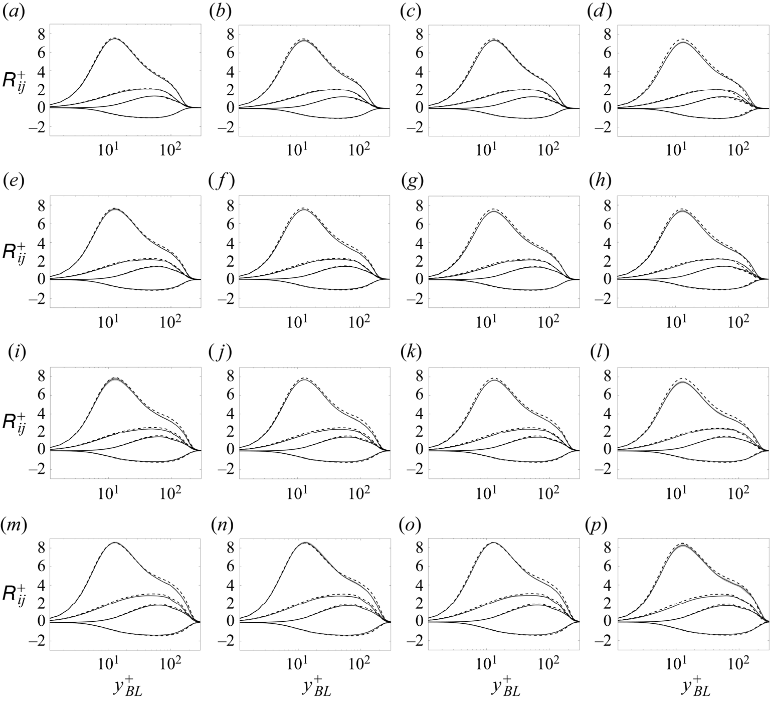
Figure 12. Variation of the Reynolds stresses  ${\mathsf{R}}_{11}$,
  ${\mathsf{R}}_{33}$,
  ${\mathsf{R}}_{22}$ and
  ${\mathsf{R}}_{12}$ with distance from the wall in RWT-0 (solid lines) compared with P-0 (dashed lines) at matched
  $(Re_\tau,\beta _{x_\tau })$ values. Rows from top to bottom correspond to different streamwise locations of
  $x'/c=0.6$,
  $0.7$,
  $0.8$ and
  $0.9$, respectively. Columns from left to right correspond to spanwise locations of the streamlines near the wall (in the collateral region) released from
  $x'_{start}/c=0.12$ (immediately downstream of the trip) at
  $z'_{start}/c=0.1$,
  $0.31$,
  $0.51$ and
  $0.72$, respectively. At each location, the Reynolds stress components are expressed in the local
  $(x_\tau,y_\tau,z_\tau )$ coordinate system aligned with the direction of wall-shear stress at that specific location. Shaded regions correspond to 80 % confidence intervals of the inner-scaled Reynolds stress profiles (due to finite time averaging), computed from the non-overlapping batch method.

Figure 13. Variation of the Reynolds stresses with wall distance at several streamwise and spanwise locations on the suction side of RWT-5 (solid lines) compared with P-2 (dashed lines) at matching  $(Re_\tau,\beta _{x_\tau })$ values. Shaded regions correspond to 80 % confidence intervals of the inner-scaled Reynolds stress profiles due to finite time averaging. See the caption of figure 12 for more details.

Figure 14. Variation of the Reynolds stresses with wall distance at several streamwise and spanwise locations on the suction side of RWT-10 (solid lines) compared with P-5 (dashed lines) at matching  $(Re_\tau,\beta _{x_\tau })$ values. Shaded regions correspond to 80 % confidence intervals of the inner-scaled Reynolds stress profiles due to finite time averaging. See the caption of figure 12 for more details.
Tables 3–5 summarise the local friction Reynolds number  $Re_\tau$ and the Clauser pressure-gradient parameters
  $\beta _{x_\tau }$ (streamwise) and
  $\beta _{z_\tau }$ (spanwise) for all the profiles plotted in figures 12–14.
Table 3. The set of three values in the numerator are  $(Re_\tau,\beta _{x_\tau },\beta _{z_\tau })$ for RWT-0 at the locations plotted in figure 12. The pair of values in the denominator are
  $(Re_\tau,\beta _{x_\tau })$ for the P-0 profiles plotted for comparison.


 Open access