1. Introduction
A fundamental challenge in wall-bounded turbulent flow is to accurately predict global properties such as friction drag. This insight is also crucial for practical scenarios as friction drag can represent up to 90 % of the total drag in maritime navigation (Schultz et al. Reference Schultz, Bendick, Holm and Hertel2011) and 50 % in aviation (Spalart & McLean Reference Spalart and McLean2011). Additionally, accurately determining the friction velocity is required for a thorough analysis of the logarithmic law (Smits Reference Smits2022). For rough surfaces, these predictions are more challenging as the impact of surface roughness is complicated (Chung et al. Reference Chung, Hutchins, Schultz and Flack2021). Thus, accurately characterizing the global properties of wall-bounded turbulence is an active research area and high-fidelity experiments and simulations are essential to advance our understanding of wall turbulence (Marusic & Monty Reference Marusic and Monty2019). For fully developed channel or pipe flows the friction velocity can be conveniently calculated using the pressure gradient. However, predicting this parameter for atmospheric boundary layers (ABLs) is more challenging and requires insight into the mean velocity gradient at the wall (Ricco & Skote Reference Ricco and Skote2022).
In contrast to canonical turbulent boundary layers, which are dominated by shear forces (Townsend Reference Townsend1976), the ABL is additionally influenced by Coriolis forces and thermal stratification (Stull Reference Stull1988). Meanwhile, the Reynolds number of ABLs can be two orders of magnitude larger than what is possible in the laboratory (Smits, McKeon & Marusic Reference Smits, McKeon and Marusic2011). Consequently, the prediction of the ABL turbulence is very challenging. In ABLs the geostrophic drag coefficient and the cross-isobaric angle can be estimated by the well-known geostrophic drag law (GDL), which was first proposed for neutral ABLs (Rossby & Montgomery Reference Rossby and Montgomery1935; Blackadar & Tennekes Reference Blackadar and Tennekes1968; Tennekes & Lumley Reference Tennekes and Lumley1972; Tennekes Reference Tennekes1973) and later extended to include the thermal stratification (Zilitinkevich Reference Zilitinkevich1969, Reference Zilitinkevich1975; Zilitinkevich & Esau Reference Zilitinkevich and Esau2002), unsteadiness (Zilitinkevich & Deardorff Reference Zilitinkevich and Deardorff1974; Arya Reference Arya1975) and baroclinicity effects (Arya & Wyngaard Reference Arya and Wyngaard1975; Arya Reference Arya1978; Hess Reference Hess2004). For convective ABLs, the updrafts tend to transit from open cells to longitudinal rolls when the surface potential temperature flux decreases and the mean wind shear increases (Salesky, Chamecki & Bou-Zeid Reference Salesky, Chamecki and Bou-Zeid2017). Recently, Tong & Ding (Reference Tong and Ding2020) derived a novel friction law for the convective ABLs in the roll-dominated regime, demonstrating that the friction velocity correlates with the mean wind speed in the mixed layer rather than with the geostrophic wind in the free atmosphere. This finding has been numerically confirmed by Liu, Gadde & Stevens (Reference Liu, Gadde and Stevens2023). For conventionally neutral ABLs, Liu, Gadde & Stevens (Reference Liu, Gadde and Stevens2021a) and Liu, Lu & Stevens (Reference Liu, Lu and Stevens2024) have updated GDL parameterizations by performing high-fidelity simulations.
When atmospheric flows are stably stratified near the surface and develop against a neutrally stratified flow above, the ABL is considered to be nocturnally stable (Zilitinkevich & Esau Reference Zilitinkevich and Esau2005). Nocturnal stable atmospheric boundary layers (NSBLs) have negative potential temperature fluxes at the surface and neutral stratification aloft. They prevail at nocturnal conditions but can also survive for several hours after sunrise over continental lands and persist continuously for days in polar regions (Mahrt Reference Mahrt2014). Their global properties (e.g. the boundary-layer height, the geostrophic drag coefficient and the cross-isobaric angle) are crucial for the heat, mass and momentum exchange between the surface and the free atmosphere. Understanding these boundary layers is of great fundamental interest and very relevant for meteorological applications (LeMone et al. Reference LeMone2019). However, so far, the understanding of NSBLs remains limited, and in this work, we therefore focus on a detailed characterization of their global properties using simulations and theoretical analysis.
In this study, we consider the NSBLs under quasi-steady, barotropic and horizontally homogeneous conditions. For simplicity, we focus on the Northern Hemisphere with latitude $\phi >0$ so that the Coriolis parameter $f = 2 \varOmega \sin \phi >0$, where $\varOmega =0.729 \times 10^{-4}\,{\rm rad}\,{\rm s}^{-1}$ is the rotation rate of the Earth. Then, it follows from dimensional analysis that the dynamics in NSBLs is governed by only two independent dimensionless parameters, e.g. the Rossby number $Ro=u_*/(f z_0)$ (Rossby & Montgomery Reference Rossby and Montgomery1935) and the Kazanski–Monin parameter $\mu =L_f/L_s$ (Kazanski & Monin Reference Kazanski and Monin1961), where $u_*$ is the friction velocity, $z_0$ is the roughness height, $L_f=u_*/f$ is the Ekman length scale (Ekman Reference Ekman1905) and $L_s=-u_*^3/(\beta q_s)$ is the surface Obukhov length (Obukhov Reference Obukhov1946) with $\beta$ denoting the buoyancy parameter and $q_s$ the surface potential temperature flux. The Rossby number characterizes the relative importance of the Coriolis force and friction drag and the Kazanski–Monin parameter $\mu$ represents the strength of thermal stratification near the surface, which varies within the interval $-10^3 < \mu < 10^3$ in the atmosphere. For $|\mu |\ll 10$ the ABL is traditionally considered neutral (Zilitinkevich & Esau Reference Zilitinkevich and Esau2002); while for $\mu =O(10^3)$, the ABL turbulence is intermittent and may no longer fully satisfy the usual conditions for the definition of turbulence (Mahrt Reference Mahrt2014). Therefore, in this study we only consider the NSBLs with $\mu = O(10)\sim O(10^2)$.
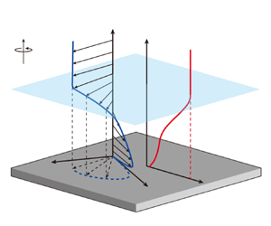
We consider the coordinate system that is oriented such that the streamwise direction is parallel to the wind direction at the surface, and the spanwise direction is orthogonal to the streamwise and vertical directions (see figure 1). Then, the GDL for the quasi-steady, barotropic and horizontally homogeneous NSBLs can be written as (e.g. Zilitinkevich & Esau Reference Zilitinkevich and Esau2005)
where $\kappa =0.4$ is the von Kármán constant, $(U_g, V_g)$ are the streamwise and spanwise components of the geostrophic wind, which are assumed to be independent of height $z$, and $A$ and $B$ are the GDL coefficients. Blackadar & Tennekes (Reference Blackadar and Tennekes1968) proved using similarity and asymptotic analysis that for neutral ABLs the $A$ and $B$ parameters are independent of the Rossby number, $Ro$. This analysis also gives that, for NSBLs, $A$ and $B$ only depend on the Kazanski–Monin parameter $\mu$, see also Zilitinkevich (Reference Zilitinkevich1975). The geostrophic drag coefficient $u_*/(U_g^2+V_g^2)^{1/2}$ and the cross-isobaric angle $\alpha _0 = \arctan (|V_g/U_g|)$ can be determined from (1.1a,b). Therefore, the $A$ and $B$ coefficients are critical in estimating available wind resources at higher elevations by extrapolating wind profiles beyond the surface layer (Gryning et al. Reference Gryning, Batchvarova, Brümmer, Jørgensen and Larsen2007; Kelly & Gryning Reference Kelly and Gryning2010). Note that similar drag relations also exist for various wall-bounded turbulent flows, such as turbulent boundary-layer flow, channel flow and pipe flow (Pope Reference Pope2000; Marusic et al. Reference Marusic, Monty, Hultmark and Smits2013). Due to the absence of Coriolis forces, the corresponding friction laws relate only to (1.1a) and are traditionally expressed through the Reynolds number.
The GDL coefficients $A$ and $B$ can be parameterized through two main approaches. One is by parameterizing the eddy viscosity profile (Rossby & Montgomery Reference Rossby and Montgomery1935; Ellison Reference Ellison1955; Krishna Reference Krishna1980; Kadantsev, Mortikov & Zilitinkevich Reference Kadantsev, Mortikov and Zilitinkevich2021), and the other is by parameterizing the mean velocity profiles (Zilitinkevich Reference Zilitinkevich1989b,Reference Zilitinkevicha; Zilitinkevich et al. Reference Zilitinkevich, Johansson, Mironov and Baklanov1998; Zilitinkevich & Esau Reference Zilitinkevich and Esau2005; Narasimhan, Gayme & Meneveau Reference Narasimhan, Gayme and Meneveau2024). Then, an asymptotic matching of the inner layer velocity profile with the outer layer is used to determine the final expressions of the GDL coefficients $A$ and $B$. For example, Kadantsev et al. (Reference Kadantsev, Mortikov and Zilitinkevich2021) derived analytical expressions for $A$ and $B$ by assuming that the eddy viscosity satisfies a linear profile in the surface layer and a constant profile in the Ekman layer. However, this eddy viscosity approximation is inconsistent with that proposed by Basu & Holtslag (Reference Basu and Holtslag2023), who derived the eddy viscosity directly from the Ekman equations by assuming a power law of the total turbulent shear stress.
Based on the assumed velocity and its gradient profiles, Zilitinkevich & Esau (Reference Zilitinkevich and Esau2005) proposed the following expressions of the GDL coefficients $A$ and $B$ for quasi-steady and barotropic NSBLs:
Here, $(a, a_0, b, b_0)$ are empirical constants, $h$ is the boundary-layer height and $(m_A, m_B)$ are the composite stratification parameters
where $(c_{fa}, c_{fb})$ are empirical constants. To obtain the values of $A$ and $B$ analytically, the boundary-layer height $h$ of quasi-steady and barotropic NSBLs is parameterized as (Zilitinkevich, Esau & Baklanov Reference Zilitinkevich, Esau and Baklanov2007)
where $(c_r, c_s)$ are empirical constants.
Given the critical importance of GDL parameterization for both theoretical research and practical applications, it is essential to investigate the GDL expressions of $A$ and $B$ for NSBLs proposed by Zilitinkevich & Esau (Reference Zilitinkevich and Esau2005). In their analysis of the GDL, Zilitinkevich & Esau (Reference Zilitinkevich and Esau2005) divided the surface layer into a logarithmic layer and a $z$-less stratification layer. Subsequently, they constructed the streamwise and spanwise velocities using the eddy viscosity approach and the assumption that the streamwise and spanwise velocity gradients above the surface layer scale as $u_*/L_s$ and $h^2 f/L_s^2$, respectively. The term ‘$z$-less stratification’ was first used by Wyngaard & Coté (Reference Wyngaard and Coté1972), which indicates that the height $z$ is no longer a primary scaling variable for very stable ABLs. However, the validity of $z$-less stratification is still an open question that requires further clarification (Grachev et al. Reference Grachev, Andreas, Fairall, Guest and Persson2013). For example, it is assumed to happen under very stable stratification (Mahrt Reference Mahrt2014), but has also been reported in weakly stable conditions (Stiperski & Calaf Reference Stiperski and Calaf2018). Note that the existence of a $z$-less stratification layer is not a prerequisite for the validity of the GDL. In other words, the division of the surface layer into a logarithmic layer and a $z$-less stratification layer is not necessary for deriving the expressions of $A$ and $B$. In addition, our analysis will show that there is no $z$-less stratification layer in the weakly stable conditions considered in this study. Therefore, removing the concept of $z$-less stratification from the analysis of the GDL may lead to a derivation that helps reveal the essential assumptions and underlying physics of the GDL.
Due to the significant challenges in atmospheric measurements (Fernando & Weil Reference Fernando and Weil2010), high-fidelity data from field experiments are very limited. With the rapid advancement of computational methods, obtaining simulation results for wall-bounded turbulent flows has now become a feasible method to produce high-fidelity data for model development. As the Reynolds number in ABLs is very high, large-eddy simulation (LES) is a widely accepted technique to model these flows (Kim & Leonard Reference Kim and Leonard2024). However, extensive datasets, covering a wide parameter range for $\mu$ and $Ro$ for NSBLs are very rare. Zilitinkevich & Esau (Reference Zilitinkevich and Esau2005) obtained their database using LES on a $64^3$ mesh and used the dynamic mixed subgrid-scale (SGS) model (Vreman, Geurts & Kuerten Reference Vreman, Geurts and Kuerten1994). Despite significant scatter, Kadantsev et al. (Reference Kadantsev, Mortikov and Zilitinkevich2021) also used this database to investigate their newly derived GDL. The grid convergence of stable ABL simulations has been investigated and was found to depend on various factors such as the wall modelling (Maronga, Knigge & Raasch Reference Maronga, Knigge and Raasch2020), the roughness length (Couvreux et al. Reference Couvreux2020), the SGS model (Dai et al. Reference Dai, Basu, Maronga and de Roode2021) and numerical schemes (Maronga & Li Reference Maronga and Li2022). Although this issue remains partially unresolved, it is widely accepted that the lowest grid level should exceed the lower limit of the inertial sublayer (Basu & Lacser Reference Basu and Lacser2017). Furthermore, Maronga & Li (Reference Maronga and Li2022) demonstrated that simulation duration is critically important to minimize the influence of inertial oscillations on the results (Van de Wiel et al. Reference Van de Wiel, Moene, Steeneveld, Baas, Bosveld and Holtslag2010). Taking these lessons into account, we have performed a unique set of simulations covering a wide range of $Ro$ and $\mu$, that facilitates a robust evaluation of GDL parameters without scatter in global flow properties.
The organization of the paper is as follows. In § 2, we discuss the simulation design. In § 3, we show that the boundary-layer height scales as $\sqrt {L_f L_s}$ and the wind gradients scale as $u_*^2/(h^2 f)$. With these physical insights, we derive the GDL coefficients $A$ and $B$ in § 4, which avoids the concept of the $z$-less stratification layer. In § 5, we show that $A$ and $B$ obtained from LES collapse to a single curve as function of $\mu$, which is well captured by the presented GDL parameterization for NSBLs given by (1.1a,b). We conclude with a summary of the main findings in § 6.
2. Large-eddy simulation framework
2.1. Governing equations
We use LES to simulate the NSBL flow over an infinite flat surface with homogeneous roughness. We integrate the spatially filtered continuity equation, momentum equation and potential temperature equation (Albertson Reference Albertson1996; Albertson & Parlange Reference Albertson and Parlange1999; Liu et al. Reference Liu, Gadde and Stevens2021a; Liu, Gadde & Stevens Reference Liu, Gadde and Stevens2021b)
where the tilde denotes spatial filtering, $\langle \boldsymbol {\cdot } \rangle$ represents horizontal averaging, $\tilde {\boldsymbol {u}}$ is the velocity, $\tilde {\boldsymbol {\omega }} = \boldsymbol {\nabla } \times \tilde {\boldsymbol {u}}$ is the vorticity, $\tilde {p}$ is the modified pressure departure from equilibrium, $\tilde {\theta }$ is the potential temperature, $\beta$ is the buoyancy parameter, $\boldsymbol {G}=(U_g, V_g, 0)$ is the geostrophic wind velocity, $\boldsymbol {\tau }$ denotes the deviatoric part of the SGS shear stress and $\boldsymbol {q}$ represents the SGS potential temperature flux. Molecular viscosity is neglected as the Reynolds number of atmospheric flows is very high.
For closure of (2.1)–(2.3), we parameterize the SGS shear stress and potential temperature flux as
where $\nu _t$ and $\nu _\theta$ are the eddy viscosity and eddy diffusivity, respectively, and $\tilde {\boldsymbol {S}}$ is the resolved strain-rate tensor with the superscript $T$ denoting a matrix transpose. We use the anisotropic minimum dissipation (AMD) model (Abkar & Moin Reference Abkar and Moin2017), which has been extensively validated (Gadde, Stieren & Stevens Reference Gadde, Stieren and Stevens2021), to perform the simulations. In the AMD model, the eddy viscosity and eddy diffusivity are determined so that the energy of the sub-filter scales of the LES solution does not increase with time.
2.2. Numerical method
Our code is an updated version of the one used by Albertson & Parlange (Reference Albertson and Parlange1999). The grid points are uniformly distributed, and the computational planes for horizontal and vertical velocities are staggered in the vertical direction. The first vertical velocity grid plane is located at the ground, and the first streamwise and spanwise velocities and potential temperature grid planes are located at half a grid distance away from the ground (Albertson Reference Albertson1996). In the vertical direction, we use a second-order finite difference method, while we use a pseudo-spectral discretization with periodic boundary conditions in the horizontal directions. Time integration is performed using the second-order Adams–Bashforth method. The projection method is used to ensure the divergence-free condition of the velocity field.
At the top boundary the vertical velocity, the SGS shear stress and the SGS potential temperature flux are enforced to zero, while the potential temperature is imposed by a constant value. In the top 25 % of the domain a Rayleigh damping layer with the damping frequency $0.001\,{\rm s}^{-1}$ determined by trial and error is applied every time step to reduce the effects of gravity waves (Klemp & Lilly Reference Klemp and Lilly1978; Liu & Stevens Reference Liu and Stevens2021). At the bottom boundary, we employ a wall model based on the Monin–Obukhov similarity theory (MOST) for both the velocity field and the potential temperature field (Monin & Obukhov Reference Monin and Obukhov1954; Moeng Reference Moeng1984; Stoll & Porté-Agel Reference Stoll and Porté-Agel2008; Liu & Stevens Reference Liu and Stevens2021)
where the overline denotes filtering at a scale of $2\Delta$ with $\Delta = (\Delta x \Delta y \Delta z)^{1/3}$ the filter scale of (2.1)–(2.3) and $\Delta x, \Delta y, \Delta z$ the grid spacings in the streamwise, spanwise and vertical directions, respectively, and where $\theta _s$ is the potential temperature at the surface, and $\psi _m$ and $\psi _h$ are, respectively, the stability corrections for the momentum and potential temperature fluxes, which for NSBLs can be parameterized as (Businger et al. Reference Businger, Wyngaard, Izumi and Bradley1971; Stull Reference Stull1988; Huang & Bou-Zeid Reference Huang and Bou-Zeid2013; Sullivan et al. Reference Sullivan, Weil, Patton, Jonker and Mironov2016; Abkar & Moin Reference Abkar and Moin2017)
Note that the definition of $L_s$ in this study is the same as Zilitinkevich & Esau (Reference Zilitinkevich and Esau2005) but different from Liu & Stevens (Reference Liu and Stevens2021), and thus the constant $\kappa$ appears in (2.6a–c). In addition, we note that the MOST, which is the basis of the wall model (2.5a,b), has been confirmed by various direct numerical simulations (e.g. Shah & Bou-Zeid Reference Shah and Bou-Zeid2014) and field experiments (e.g. Businger et al. Reference Businger, Wyngaard, Izumi and Bradley1971). Since the MOST is generally valid in the surface layer of the ABLs in weakly stable regime (Grachev et al. Reference Grachev, Fairall, Persson, Andreas and Guest2005; Katul, Konings & Porporato Reference Katul, Konings and Porporato2011; Stoll et al. Reference Stoll, Gibbs, Salesky, Anderson and Calaf2020), the wall model based on the MOST is used in this study.
2.3. Computational set-up
To obtain simulation results independent of the computational domain, the domain size in each direction has to be several times the size of the largest eddies or the boundary-layer height (Couvreux et al. Reference Couvreux2020). The selected computational domain size is $800\,{\rm m}\times 800\,{\rm m}\times 800\,{\rm m}$ in the streamwise, spanwise and vertical directions, respectively. As shown in table 1, the deepest boundary-layer height is approximately 266 m, which is less than one third of the computational domain size. Since the MOST-based wall model is employed, the lowest grid level $z_1$ should be above the lower limit of the inertial sublayer $z_*$ (Basu & Lacser Reference Basu and Lacser2017). The parameter $z_*$ can be related to the roughness length $z_0$, and their ratio depends on the atmospheric stability. In particular, for stably stratified conditions, the ratio $z_*/z_0$ for the wind profile was found to be significantly lower, approximately in the range of $11 \sim 55$ (Garratt Reference Garratt1983; Basu & Lacser Reference Basu and Lacser2017). Meanwhile, $z_1$ should be below the upper limit of the inertial sublayer, i.e. the Ozmidov length $L_O=(\varepsilon /N^3)^{1/2}$, where $\varepsilon$ is the mean viscous dissipation and $N$ is the Brunt–Väisälä frequency (Dougherty Reference Dougherty1961; Ozmidov Reference Ozmidov1965; Huang & Bou-Zeid Reference Huang and Bou-Zeid2013; Sullivan et al. Reference Sullivan, Weil, Patton, Jonker and Mironov2016). We select the grid resolution as $192\times 192\times 201$ such that the grid is nearly isotropic (Gadde et al. Reference Gadde, Stieren and Stevens2021), and, more importantly, $z_1/z_0\ge 20$ since $z_0 \le 0.1$ m (see table 1). At the same time, this grid also satisfies the grid resolution requirement $z_1/L_O<1$ (see figure 3 below).
The simulations are initialized with a constant potential temperature $\theta =265$ K and a constant geostrophic wind speed $G=8\sim 12\,{\rm m}\,{\rm s}^{-1}$. Turbulence is triggered by adding random perturbations. A random noise term with a magnitude of $3\,\%$ of the geostrophic wind speed is added to velocities below $50$ m, and for the potential temperature a noise term with an amplitude of $0.1$ K is added. The reference temperature is set to $\theta _0=263.5$ K. The latitude $\phi$ varies between $30^\circ$ and $73^\circ$, and the surface cooling rate is set to $C_r=0.05\sim 0.35\,{\rm K}\,{\rm h}^{-1}$. The roughness length is $z_0=0.001\sim 0.1$ m. To remove the effects of slowly decaying inertial oscillations on the top of the domain (Van de Wiel et al. Reference Van de Wiel, Moene, Steeneveld, Baas, Bosveld and Holtslag2010; Maronga & Li Reference Maronga and Li2022), the initial transient period lasts for 1.5 inertial time periods and the statistics are collected over the following one inertial period, i.e. $ft \in [3{\rm \pi}, 5{\rm \pi} ]$ (see figure 2). This ensures the flow has reached its quasi-stationary state and the changes of $u_*$ and $\alpha _0$ are less than 5 % of their mean values (see figure 2). We note that many time steps ($\sim O(10^7)$) are required to resolve the large range of relevant time scales in the problem, spanning from small-scale turbulence to large-scale inertial oscillations. A summary of these simulations is given in table 1, where the cases are arranged such that the value of $\phi$ increases monotonically from upper to lower rows.
We remark that the simulation input parameters of case 20 are the same as the standard Global Energy and Water Cycle Experiment Atmospheric Boundary Layer Study case (Beare et al. Reference Beare2006; Liu & Stevens Reference Liu and Stevens2021), with the only exception being that the free-atmosphere lapse rate has been set as zero to ensure the flow belongs to the NSBL regime (Maronga et al. Reference Maronga, Knigge and Raasch2020). Besides, we remark that the simulations of Zilitinkevich & Esau (Reference Zilitinkevich and Esau2005) that will be used for comparison were performed for $ft=2.1{\rm \pi}$, with time averaging over the period $ft\in [1.3{\rm \pi}, 2.1{\rm \pi} ]$. As shown in figure 2, a time averaging should start around $ft \approx 3{\rm \pi}$ to ensure reliable determination of the friction velocity $u_*$ and the cross-isobaric angle $\alpha _0$. This is the main reason for the large scatter of the simulation data of Zilitinkevich & Esau (Reference Zilitinkevich and Esau2005). In contrast, the simulation data obtained from our LES with much longer simulation time show very limited scatter (see below).
It is well known that sufficient grid resolution is important in simulating stable ABLs with low turbulence levels (Huang & Bou-Zeid Reference Huang and Bou-Zeid2013; Maronga & Li Reference Maronga and Li2022). Therefore, a quantitative investigation into the appropriateness of the chosen grid resolution is performed. Figure 3 shows that for all simulated cases the ratio $z_1/L_O <1$, which justifies the use of the MOST-based wall model. Similar to Sullivan et al. (Reference Sullivan, Weil, Patton, Jonker and Mironov2016), figure 3 shows that the Ozmidov length $L_O$ decreases as the cooling rate $C_r$ increases. Thus, if a much larger cooling rate, e.g. $C_r=2.5\,{\rm K}\,{\rm h}^{-1}$ (Huang & Bou-Zeid Reference Huang and Bou-Zeid2013), is considered, a higher grid resolution may be needed. However, for the cooling rate range $C_r=0.05\sim 0.35\,{\rm K}\,{\rm h}^{-1}$ considered here, the chosen grid resolution meets the required standards.
To further illustrate the effect of grid resolution on simulation results, figure 4 shows the mean vertical profiles of the wind speed, potential temperature, total shear stress and potential temperature flux for case 2 in table 1, which has the largest value of $\mu =193.3$ and hence may have the strongest dependence on the grid resolution. The figure indicates that the magnitudes of the total shear stress and potential temperature flux in the boundary layer, as well as the boundary-layer height, decrease slightly as the grid resolution increases. This lack of strictly grid convergence in LES of the stable boundary layer is well known and remains partially unresolved (Maronga & Li Reference Maronga and Li2022). Nevertheless, figure 4 shows that the mean vertical profiles with medium and dense grid resolutions do not change significantly. This finding confirms the appropriateness of the adopted grid resolution of $192\times 192\times 201$ in this study.
3. Boundary-layer height and wind gradient profiles
3.1. Boundary-layer height
In stable ABL flows the profile of the magnitude of total turbulent shear stress $\tau$ is often expressed as follows (Nieuwstadt Reference Nieuwstadt1984; Sorbjan Reference Sorbjan1986; Basu & Holtslag Reference Basu and Holtslag2023):
We remark that (3.1) was proposed under quasi-steady, barotropic and horizontally homogeneous conditions (Nieuwstadt Reference Nieuwstadt1984). Thus, it might not be valid for unsteady (Mahrt Reference Mahrt2014; Momen & Bou-Zeid Reference Momen and Bou-Zeid2017), baroclinic (Arya & Wyngaard Reference Arya and Wyngaard1975; Floors, Peña & Gryning Reference Floors, Peña and Gryning2015; Momen et al. Reference Momen, Bou-Zeid, Parlange and Giometto2018) or surface heterogeneous (Schmid et al. Reference Schmid, Lawrence, Parlange and Giometto2019; Cooke, Jerolmack & Park Reference Cooke, Jerolmack and Park2024) flows. In addition, we remark that many different definitions of the stable ABL height $h$ are available in literature, such as (a) the layer through which surface-based turbulence extends, (b) the top of the layer with downward potential temperature flux, (c) the height of the low-level jet and (d) the top of the potential temperature inversion layer (Vickers & Mahrt Reference Vickers and Mahrt2004).
In this study, we adopt definition (a). Specifically, the boundary-layer height $h$ is defined as the height at which the total shear stress first vanishes. In particular, $h$ is proportional to the height $h_{0.05}$, where the total shear stress reduces to 5 % of its surface value (van Dop & Axelsen Reference van Dop and Axelsen2007; Liu et al. Reference Liu, Gadde and Stevens2021b)
By utilizing his local scaling hypothesis and the constant assumption of the flux Richardson number, Nieuwstadt (Reference Nieuwstadt1984) determined analytically that the exponent $\alpha = 3/2$. Note that the value of $\alpha$ may not be a universal constant and other values of $\alpha$ have also been reported in the literature (Caughey, Wyngaard & Kaimal Reference Caughey, Wyngaard and Kaimal1979; Yokoyama, Gamo & Yamamoto Reference Yokoyama, Gamo and Yamamoto1979; Lacser & Arya Reference Lacser and Arya1986; Sorbjan Reference Sorbjan1986; Lenschow et al. Reference Lenschow, Li, Zhu and Stankov1988; Byun Reference Byun1991; Delage Reference Delage1997).
Figure 5 shows the profile of normalized total turbulent shear stress in NSBLs. The open circles are the simulation data from table 1, the open triangles are the field data taken from Nieuwstadt (Reference Nieuwstadt1984), the open inverted triangles are the field data of Wittich (Reference Wittich1991) and the solid line is the prediction of (3.1) with $\alpha =3/2$. The good agreement of simulation data with field measurements validates our simulation results. Furthermore, our simulations indicate that the 3/2-law of total turbulent shear stress proposed by Nieuwstadt (Reference Nieuwstadt1984) describes the data across the entire parameter range considered here.
For NSBLs with large values of $\mu$, the parameterization of the boundary-layer height $h$ given by (1.4) can be approximated as
where $c_s$ is the Zilitinkevich constant (Derbyshire Reference Derbyshire1990), which depends on the definition of the boundary-layer height $h$. Equation (3.3) was originally proposed by Zilitinkevich (Reference Zilitinkevich1972) based on boundary-layer scaling arguments and implies that the boundary-layer height $h$ scales as $\sqrt {L_f L_s}$. Based on this definition, Zilitinkevich (Reference Zilitinkevich1989b) summarized $c_s$ from several studies and found it to vary between 0.55 and 1.58. This large variation affects the values of other empirical constants in the GDL formulation of Zilitinkevich & Esau (Reference Zilitinkevich and Esau2005). As shown below, this is not the case for our formulation, where only the scaling of (3.3) matters while the value of $c_s$ is irrelevant. This is also the case for the value of $\alpha$ since it can be absorbed into $c_s$, see (3.2) and (3.3). Recently, Basu & Holtslag (Reference Basu and Holtslag2023) derived two different eddy viscosity profile formulations, both leading to the boundary-layer height parameterization of Zilitinkevich (Reference Zilitinkevich1972). The two derivations give $c_s=0.922$ and $c_s=0.658$, respectively, and they argued that the Zilitinkevich constant $c_s=0.658$ seems to be a better option. More recently, Narasimhan et al. (Reference Narasimhan, Gayme and Meneveau2024) also reported $c_s=0.78$ based on their LES data.
Figure 6 compares the dimensionless boundary-layer height $h/L_f$ obtained from the present simulations of table 1 (filled circles), the simulation data of Zilitinkevich et al. (Reference Zilitinkevich, Esau and Baklanov2007) (open circles) and the prediction of (3.3) with $c_s=0.62$, which is determined using a least-squares fitting procedure based on the present LES database. All symbols collapse to a single curve, indicating that the dimensionless boundary-layer height $h/L_f$ indeed only depends on the Kazanski–Monin parameter $\mu$. The good agreement between the simulation data and theoretical prediction confirms the validity of the boundary-layer height parameterization of (3.3) over a much wider range of $\mu$ than Zilitinkevich et al. (Reference Zilitinkevich, Esau and Baklanov2007) considered. Note that the simulation data of Zilitinkevich et al. (Reference Zilitinkevich, Esau and Baklanov2007), which have a smaller range of $\mu$ than the present study, are very close to our theoretical model and simulation results.
3.2. Wind gradient profiles
Recall that we focus on the quasi-steady and barotropic NSBLs in weakly stable regime, whose dynamics is governed by the Ekman equations
where $\tau _x$ and $\tau _y$ are the horizontally averaged streamwise and spanwise turbulent shear stresses. The vertical derivative of (3.4a,b) is
where $\xi =z/h$ is the normalized coordinate. Since the total turbulent shear stresses nearly collapse onto a single curve as a function of $z/h$, see (3.1) and figure 5, it is intuitive to conjecture that the wind gradients $\textrm {d} U/\textrm {d} z$ and $\textrm {d} V/\textrm {d} z$ normalized with $u_*^2/(h^2 f)$ should also approximately collapse. To confirm this conjecture, figure 7 shows the streamwise and spanwise velocity gradients normalized by $u_*^2/(h^2 f)$. Both tend to collapse to a single curve and are $O(1)$ above the surface layer. This indicates that $u_*^2/(h^2 f)$ is indeed the appropriate scaling for the wind gradients above the surface layer (Lin & Segel Reference Lin and Segel1988). Additionally, neither $\textrm {d} U/\textrm {d} z$ nor $\textrm {d} V/\textrm {d} z$ shows a uniform region, i.e. a region independent of $z$. This indicates that a $z$-less stratification layer is absent in NSBLs in the studied parameter range of $\mu$ and $Ro$.
To quantify the effectiveness of the scaling $u_*^2/(h^2 f)$, figure 8 shows the mean absolute error (MAE) of the wind gradient profiles in figure 7. Here, the MAE is calculated as
where $X=(h^2 f/u_*^2)(\textrm {d} U/\textrm {d} z)$ and $(h^2 f/u_*^2)(\textrm {d} V/\textrm {d} z)$, $\bar {X}$ is the sample mean (i.e. the average of all cases) profile of $X$ (see figure 7), $i$ is the case number and $n=20$ is the total number of all simulated cases (see table 1). Figure 8 shows clearly that the MAEs of wind gradients normalized by the scaling $u_*^2/(h^2 f)$ are $O(0.1)$ above the surface layer. This quantitatively confirms the effective collapse of the wind gradients by the scaling $u_*^2/(h^2 f)$ in the studied parameter range.
We remark that Zilitinkevich & Esau (Reference Zilitinkevich and Esau2005) assumed that the wind gradients $\textrm {d} U/\textrm {d} z$ and $\textrm {d} V/\textrm {d} z$ above the surface layer scale as $u_*/L_s$ and $h^2 f/L_s^2$, respectively. For NSBLs with large values of $\mu$, we have shown that the boundary-layer height $h$ scales as $\sqrt {L_f L_s}$, see (3.3) and figure 6. Under this condition, the scalings $u_*/L_s$, $h^2 f/L_s^2$ and $u_*^2/(h^2 f)$ are equivalent since
However, choosing the scaling $u_*^2/(h^2 f)$ may still be more convenient in practice, as it is directly derived from the vertical derivatives of the Ekman equations (3.5a,b) and hence ensures the normalized wind gradients above the surface layer are $O(1)$. In addition, for smaller values of $\mu$, the difference between these scalings may exist since the boundary-layer height $h$ ceases to scale as $\sqrt {L_f L_s}$ but scales as $L_f$.
4. Theoretical model
In this section, we will derive the analytical expressions of the GDL coefficients $A$ and $B$ for NSBLs under quasi-steady, barotropic and horizontally homogeneous conditions.
4.1. Analytical expression of A
We first determine the analytical expression of the GDL coefficient $A$. In the surface layer, of which the height is typically approximately 10 % of the boundary-layer height $h$ (Basu & Lacser Reference Basu and Lacser2017), the mean streamwise velocity $U$ is assumed to be described by the MOST (Monin & Obukhov Reference Monin and Obukhov1954; Businger et al. Reference Businger, Wyngaard, Izumi and Bradley1971)
where $c_\psi$ is an empirical constant and, according to (2.6a–c), $c_\psi = 4.8 \kappa$ in this study. Note that (4.1) is also the basis of the wall model employed in the current LES.
Above the surface layer or in the Ekman layer, figure 7(a) shows that the streamwise velocity gradient $\textrm {d} U/\textrm {d} z$ scales as $u_*^2/(h^2 f)$. Thus, we can assume
where $f_u$ is independent of $Ro$ and $\mu$. Integrating (4.2) from below to the top of the boundary layer and noting that $L_f=u_*/f$, we find
We further assume the mean streamwise velocity $U$ given by (4.1) and (4.3) matches at the interface $\xi =L_s/(c_1 h)$ or $z=L_s/c_1$, where $c_1$ is an empirical constant. Thus, by substituting (4.1) into (4.3), we find
Finally, substituting (1.1a) and (3.3) into (4.4) and noting that $\mu =L_f/L_s$, we obtain
where
Without knowing the form of $f_u$, the analytical expression of $a_1$ and thus of $A$ cannot be obtained. However, figures 6, 7(a) and 9 indicate that $c_s = O(1)$, $c_1=O(1)$ and $f_u=O(1)$ above the surface layer. Thus, $\textrm {d} a_1/\textrm {d} \mu = f_u / (2 c_1 c_s^2 \mu ^{3/2}) = O(\mu ^{-3/2})= O(10^{-3})$ when $\mu =O(10^2)$, indicating that $a_1$ depends only very weakly on $\mu$ and hence can be assumed as a constant for simplicity. In this sense, the analytical expression of $A$ is given by (4.5), which involves only two empirical constants $(a_1, c_1)$ or equivalently $(a_1, a_2)$. Note that (4.5) has the same structure as equation (24) of Zilitinkevich & Esau (Reference Zilitinkevich and Esau2005). However, in our derivation we divide the boundary layer only into the surface layer and the Ekman layer, and requiring a $z$-less stratification layer is unnecessary. This makes the physics underlying the GDL more clear: it is a direct result of the asymptotic matching of the velocity profile between the surface layer and the Ekman layer. In addition, by making a comparison between (1.2a) and (4.5), we see the term $\ln (a_0 + m_A)$ in (1.2a) should be $a_0 + \ln m_A$. In this way, (1.2a) in the limit $\mu \gg 10$ approaches $A = \ln \mu - a c_s \sqrt {\mu } + a_0$, which is the same as (4.5) if $a c_s =a_1$ and $a_0 =a_2$.
4.2. Analytical expression of B
To determine the analytical expression of $B$, we recall that
where $\tau _y$ is the spanwise component of the total shear stress tensor. We focus on the surface layer. Then, by substituting (1.1a) and (4.1) into (4.7) we obtain
The bottom boundary condition of (4.8) is $\tau _y(0)=0$. Integrating (4.8) from 0 to $z$, one obtains
In the surface layer the eddy viscosity approach is assumed to be valid, such that (Zilitinkevich & Esau Reference Zilitinkevich and Esau2005)
where $V$ is the mean spanwise velocity. We remark that there is an extensive discussion in the literature about the eddy viscosity approach used here (see, e.g. Constantin & Johnson Reference Constantin and Johnson2019), where the eddy viscosity $K_m$ can be a function of height (Grisogono Reference Grisogono1995), stability (Nieuwstadt Reference Nieuwstadt1983) and baroclinicity (Berger & Grisogono Reference Berger and Grisogono1998). In these studies, the velocity profiles were derived based on assumed $K_m$ profiles. However, correct $K_m$ profiles in the whole boundary layer are very difficult to obtain and sometimes the eddy viscosity approach itself might become invalid in some regions of the boundary layer (Liu & Stevens Reference Liu and Stevens2022; Liu et al. Reference Liu, Gadde and Stevens2023). Because the eddy viscosity approach is generally valid in the surface layer, it is adopted here. In particular, in the surface layer $K_m$ in (4.10) is determined from (4.1) and the approximation $K_m {\rm d} U/{\rm d}z \approx u_*^2$.
By combining (4.9) and (4.10), we find
The bottom boundary condition of (4.11) is $V(0)=0$. By integrating (4.11) from 0 to $z$ one can determine the mean spanwise velocity $V$ in the surface layer as
Above the surface layer, figure 7(b) shows that the spanwise velocity gradient $\textrm {d} V/\textrm {d} z$ scales as $u_*^2/(h^2 f)$ for NSBLs in the studied parameter range of $Ro$ and $\mu$. Thus, similar to the derivation of $A$, we can assume
where $f_v$ is independent of $Ro$ and $\mu$. Integrating (4.13) from below to the top of the boundary layer and noting that $L_f=u_*/f$, we obtain
We further assume the mean spanwise velocity $V$ given by (4.12) and (4.14) matches at the interface $\xi =L_s/(c_2 h)$ or $z=L_s/c_2$, where $c_2$ is an empirical constant. Thus, by substituting (4.12) into (4.14) and noting that $\mu =L_f/L_s$, we obtain
Substituting (1.1b), (3.3) and (4.5) into (4.15), we find
where
Finally, since the final term on the right-hand side of (4.16) is much smaller than the other two terms for $\mu \gg 10$, (4.16) can be written as
Similar to $a_1$ we can assume $b_1$ to be constant. Therefore, the analytical expression of $B$ is given by (4.16), which also involves two empirical constants $(b_1, c_2)$ since $(a_1, c_1)$ are already given by (4.5). Note that (4.18) is different from equation (37) of Zilitinkevich & Esau (Reference Zilitinkevich and Esau2005). The reason is as follows: in their derivation Zilitinkevich & Esau (Reference Zilitinkevich and Esau2005) divided the surface layer into a logarithmic layer and a $z$-less stratification layer, and determined the spanwise velocity in the $z$-less stratification layer by only keeping the term proportional to $z^2$. This leads to a discontinuity of the spanwise velocity across the interface of the logarithmic layer and the $z$-less stratification layer. As a result, their obtained equation (37) only included a single term similar to $b_1 \sqrt {\mu }$, which underestimates the values of $B$ for small and moderate $\mu$ and thus a correction constant $b_0$ is introduced to their general expression of $B$ in (1.2b). Actually, (1.2b) reduces to $B = b c_s^3 \sqrt {\mu } + b_0 c_s / \sqrt {\mu }$ in the limit $\mu \gg 10$, which is the same as (4.18) when $b c_s^3 = b_1$ and $b_0 c_s=b_2$. Because we treat the surface layer as a whole, the continuity of the spanwise velocity is satisfied automatically. As a result, our derivation gives a higher-order term, and hence, there is no need to introduce an additional correction constant. The effectiveness of this treatment also reveals the essential physics of the GDL more clearly.
4.3. Further remarks
We remark that when deriving the analytical expressions of $A$ and $B$, i.e. (4.5) and (4.16) we have made two ansatzes: first, the streamwise and spanwise velocity profile between the inner and outer layers matches at a dimensionless height $1/(c_1c_s\sqrt {\mu })$ and $1/(c_2c_s\sqrt {\mu })$, respectively; and second, $a_1$ and $b_1$ can be approximated as constants that are independent of $\mu$. These ansatzes enable us to predict well $(A, B)$ without knowing the forms of $(f_u, f_v)$ and with reasonable values of $(c_1, c_2)$, see § 5 below. This fact also verifies the ansatzes themselves. However, if one assumes that the streamwise and spanwise velocity profiles between the inner and outer layers match at dimensionless heights independent of $\mu$, then one would find these heights are too close to the top of boundary layer, and therefore, this assumption should be abandoned. On the other hand, if one assumes that $a_1$ and $b_1$ can be expanded in power series of $1/\sqrt {\mu }$, then the values of $(c_1, c_2)$ cannot be determined without knowing the forms of $(f_u, f_v)$ and thus this assumption should also be discarded. We further remark that the two velocities $U_g$ and $V_g$ can be obtained by substituting (4.5) and (4.16) into (1.1a,b). At first sight, these two velocities seem to be expressed to different orders of $\mu$. However, we emphasize that the high-order term in $B$ or $V_g$ is obtained directly by ensuring the continuity of the spanwise velocity at the matching height, which differs from the formal asymptotic expansion. We also emphasize that, since (4.5) and (4.16) predict $(A,B)$ accurately, they also predict well $(U_g, V_g)$ and hence the geostrophic drag coefficient and the cross-isobaric angle.
5. Results and discussion
5.1. The performance of the analytical expressions of A and B
Figure 9 compares the GDL coefficient $A$ as obtained from the theoretical predictions and simulation results of the present study with those of Zilitinkevich & Esau (Reference Zilitinkevich and Esau2005). The results indicate that $A$ decreases monotonically with increasing $\mu$. The present simulation data (filled circles) collapse well onto a single curve and have much less scatter than the Zilitinkevich & Esau (Reference Zilitinkevich and Esau2005) data. We remark that the simulation data of Zilitinkevich & Esau (Reference Zilitinkevich and Esau2005) were averaged over the period $ft\in [1.3{\rm \pi}, 2.1{\rm \pi} ]$. Because the flow above the boundary layer is neutrally stratified, the boundary layer is still developing during this period (figure 2). Thus, the simulation duration and time-averaging period should be the main reasons for their large scatter, although various other aspects such as the grid resolution, SGS model and numerical scheme may also have made some contributions. Even though their simulation data (open circles) display significant scatter, the overall trend agrees with ours (filled circles). These observations confirm the validity of the GDL for NSBLs described by (1.1a) within LES, extending its applicability across a wider range of $\mu$.
In figure 9, the theoretical predictions are obtained by (1.2a) with the empirical constants $(a, a_0, c_{fa}, c_r, c_s)=(1.4, 1.65, 1, 0.6, 0.51)$ proposed by Zilitinkevich & Esau (Reference Zilitinkevich and Esau2005) (dashed line), and (4.5) with $(a_1, c_1)=(0.72, 2.25)$ determined from the present LES database using a least-squares fitting procedure (solid line). The theoretical prediction of Zilitinkevich & Esau (Reference Zilitinkevich and Esau2005) somewhat overestimates $A$, especially for small $\mu$, and approaches asymptotically to the theoretical prediction of the present study for very large $\mu$. The latter fact is consistent with our analysis given at the end of § 4.1, where we conclude that these two parameterizations are equivalent in the limit $\mu \gg 10$ if $a c_s =a_1$. Here, $a=1.4$ and $c_s=0.51$, and thus $a c_s =0.71 \approx a_1=0.72$. The prediction of (4.5) agrees well with both the simulation data of the present study and those of Zilitinkevich & Esau (Reference Zilitinkevich and Esau2005). This validates the present parameterization of $A$ given by (4.5) with only two empirical constants $(a_1, c_1)$ in the studied parameter range of $\mu$ and $Ro$. We remark that the surface-layer height normalized by the boundary-layer height can be approximated as $L_s/(c_1 h) = 1/(c_1 c_s \sqrt {\mu })$, which decreases as $\mu$ increases. In particular, it varies within the range of 5 %–17 % in the present simulations since $c_1=2.25$ (figure 9), $c_s=0.62$ (figure 6) and $\mu \in [17, 193]$ (table 1). In addition, we remark that the empirical constants $(a, a_0, c_{fa}, c_r, c_s)=(1.4, 1.65, 1, 0.6, 0.51)$ proposed by Zilitinkevich & Esau (Reference Zilitinkevich and Esau2005) were optimized using their LES data. If optimized using our LES data, the prediction of (1.2a) matches well with our LES results (data not shown). This agreement is expected, as (1.2a) has five adjustable constants. In contrast, (4.5) has only two adjustable parameters and the main physics is clearer. The comparison of these two expressions thus indicates that high-fidelity data are necessary to obtain accurate parameterization of GDL coefficients.
Figure 10 compares the GDL coefficient $B$ obtained from theoretical predictions and simulation results of the present study and of Zilitinkevich & Esau (Reference Zilitinkevich and Esau2005). The simulation results indicate that $B$ increases monotonically as $\mu$ increases. The present simulation data collapse well to a single curve, and hence validate the GDL for NSBLs over a wider range of $\mu$. For small $\mu \lesssim 40$, the simulation data of Zilitinkevich & Esau (Reference Zilitinkevich and Esau2005) agree well with our simulation results. For $\mu \gtrsim 40$ there is relatively large scatter in their data and $B$ is significantly larger than in the present study (figure 10). As mentioned in § 2.3, the simulations conducted by Zilitinkevich & Esau (Reference Zilitinkevich and Esau2005) were limited to $ft=2.1{\rm \pi}$, which does not allow for reliable determination of the friction velocity $u_*$ and the cross-isobaric angle $\alpha _0$. Given that $B=(\kappa G/u_*) \sin \alpha _0$ is sensitive to changes in $u_*$ and $\alpha _0$, this limitation likely contributed to their overestimation of $B$.
In figure 10, the theoretical predictions are obtained by (1.2b) with the empirical constants $(b, b_0, c_{fb}, c_r, c_s)=(10, -2, 1, 0.6, 0.51)$ proposed by Zilitinkevich & Esau (Reference Zilitinkevich and Esau2005) (dashed line), and (4.18) with $(b_1, c_2)=(1.02, 0.86)$ determined from the present LES database using a least-squares fitting procedure (solid line). The theoretical prediction of Zilitinkevich & Esau (Reference Zilitinkevich and Esau2005) underestimates $B$ for small $\mu$ and overestimates $B$ for large $\mu$. The latter fact is consistent with our analysis given at the end of § 4.2, where we conclude that these two parameterizations are equivalent in the limit $\mu \gg 10$ if $b c_s^3 =b_1$. Here, $b=10$ and $c_s=0.51$, and thus $b c_s^3 =1.33 > b_1=1.02$, indicating that the prediction of (1.2b) becomes larger than that of (4.18) at large $\mu$. The present prediction of (4.18) agrees well with all the simulation data of the present study. This validates the present parameterization of $B$ given by (4.18) with only two empirical constants $(b_1, c_2)$ in the studied parameter ranges of $\mu$ and $Ro$. In addition, figure 10 shows that the term $b_1 \sqrt {\mu }$ approximates $B$ well for large values of $\mu$ (blue dashed-dotted line). However, there are deviations between $b_1 \sqrt {\mu }$ (blue dashed-dotted line) and $B$ (solid line) for lower values of $\mu$. The purpose of the term $b_2/\sqrt {\mu }$ (yellow dashed-dotted line) is to model these differences for lower $\mu$.
5.2. The geostrophic drag coefficient and cross-isobaric angle
Figure 11 compares the geostrophic drag coefficient $u_*/G$ and the cross-isobaric angle $\alpha _0=\arctan (|V_g/U_g|)$ obtained from the present simulations with the GDL given by (1.1a,b), where the GDL coefficients $A$ and $B$ are parameterized by (4.5) and (4.18) using the empirical constants $(a_1, b_1, c_1, c_2)=(0.72, 1.02, 2.25, 0.86)$ determined in § 5.1. The figure shows that the agreement between the new parametrizations and all the numerical data is good. Figure 11(a) shows that our simulations cover the range $0.0195 \leq u_*/G \leq 0.0304$, which covers the typical range observed in atmospheric measurements. Figure 11(b) shows that the cross-isobaric angle varies between $23^\circ$ and $44^\circ$ and that all LES data collapse to the theoretical curve. This good agreement is expected as $\alpha _0=\arcsin [(B u_*)/(\kappa G)]$ and $B$ (figure 9b) and $u_*/G$ (figure 11a) have already been predicted accurately. Note that the cross-isobaric angle $\alpha _0$ in NSBLs (see table 1 and figure 11b) is usually larger than that in conventionally neutral (Liu et al. Reference Liu, Gadde and Stevens2021a) and convective ABLs (Liu et al. Reference Liu, Gadde and Stevens2023). This is a typical phenomenon in ABLs: the wind veer is stronger in stable conditions than in neutral and convective conditions.
The geostrophic drag coefficient $u_*/G$ and the cross-isobaric angle $\alpha _0$ are two key global properties of ABLs, which are fundamental for constructing wind profiles throughout the entire turbulent boundary layer. Therefore, we present the geostrophic drag coefficient $u_*/G$ and the cross-isobaric angle $\alpha _0 = \arctan (|V_g/U_g|)$ in figure 12. The simulation results (filled circles) are in good agreement with the GDL results (solid lines), see also figure 11. The figure demonstrates that $u_*/G$ decreases with increasing $Ro$ or $\mu$. Notably, $u_*/G$ exhibits a strong dependence on $Ro$ for low $\mu$ (e.g. $\mu =15$) and becomes nearly independent of $Ro$ for high $\mu$ (e.g. $\mu =200$). Furthermore, figure 12(b) illustrates that $\alpha _0$ decreases with increasing $Ro$, and increases with increasing $\mu$. The dependence of $\alpha _0$ on $Ro$ is more pronounced for lower $\mu$.
6. Conclusions
We investigate numerically and theoretically the global properties of NSBLs under quasi-steady, barotropic and horizontally homogeneous conditions. In particular, we focus on NSBLs with the Kazanski–Monin parameter $\mu =O(10)\sim O(10^2)$ since they are considered neutral when $|\mu |\ll 10$ and may be intermittent when $\mu \gg 10^2$. To get high-fidelity data for NSBLs, we perform a series of carefully designed LESs with sufficiently high grid resolutions and for long time durations. These simulations cover a wider range of the Kazanski–Monin parameter $\mu \in [16.7, 193.3]$ and the Rossby number $Ro \in [1.68\times 10^4, 2.42 \times 10^6]$ than previously considered. We find that the boundary-layer height $h$ scales as $\sqrt {L_f L_s}$, and both the streamwise and spanwise wind gradients scale as $u_*^2/(h^2 f)$, where $L_f$ is the Ekman length scale, $L_s$ is the surface Obukhov length, $u_*$ is the friction velocity and $f$ is the Coriolis parameter.
We study the GDL for NSBLs to obtain an analytical prediction for the global properties like the geostrophic drag coefficient $u_*/G$ and the cross-isobaric angle $\alpha _0$ as a function of the Kazanski–Monin parameter $\mu$ and the Rossby number $Ro$. We first show that the GDL coefficients $A$ and $B$ obtained from carefully performed LES collapse to single curves as functions of $\mu$. This verifies the GDL for NSBLs over an extended range of $\mu$ within LES. We emphasize that the present LES employs the wall model based on the MOST (Monin & Obukhov Reference Monin and Obukhov1954). Thus, the concept of ‘grid convergence’ does not strictly apply here. For example, the magnitude of total shear stress and potential temperature flux at the surface decrease as the grid resolution increases. This grid-sensitivity issue should be kept in mind when one compares the LES results with direct numerical simulations and experimental measurements. In addition, because the MOST is not valid for very stable boundary layers with $\mu \gg O(10^2)$, the current LES is unable to simulate these cases. Therefore, to verify the GDL for NSBLs over the whole range of $\mu$ using high-fidelity LES data, one may need to utilize a partially wall-resolved LES (Chinita, Matheou & Miranda Reference Chinita, Matheou and Miranda2022).
We derived new analytical expressions of $A$ and $B$ by using three crucial insights: (i) the boundary-layer height can be parameterized by the approach of Zilitinkevich (Reference Zilitinkevich1972), (ii) the wind gradients can be scaled by $u_*^2/(h^2 f)$ and (iii) the streamwise and spanwise velocities are continuous in the boundary layer. In addition, we assume that the eddy viscosity approach is valid in the surface layer and the mean streamwise velocity therein can be predicted by the MOST (Monin & Obukhov Reference Monin and Obukhov1954). This allows a direct derivation, without the need to assume $z$-less stratification, of analytical expressions for $A$ (4.5) and $B$ (4.18) with just four empirical constants. These constants can be determined from measurements or simulations, and here we use the latter. The good agreement between the theoretical predictions and the simulation results confirms the validity of the new analytical expressions of $A$ and $B$ for the studied range of $\mu$ and $Ro$.
The drag law exists in various wall-bounded turbulent flows, which may have different formulations in different flows. For example, it manifests as the friction law in channel and pipe flows (Pope Reference Pope2000), the convective logarithmic friction law in convective boundary layers (Tong & Ding Reference Tong and Ding2020; Liu et al. Reference Liu, Gadde and Stevens2023) and the GDL in neutral and stable boundary layers (Zilitinkevich & Esau Reference Zilitinkevich and Esau2005; Liu et al. Reference Liu, Gadde and Stevens2021a). Physically, the existence of drag law is a direct result of the asymptotic matching of the velocity profiles between the inner and outer layers (Zilitinkevich Reference Zilitinkevich1975). From this perspective, our results not only advance our physical understanding of the GDL for NSBLs, but also can be very helpful for deepening our understanding of wall turbulence in general (Smits et al. Reference Smits, McKeon and Marusic2011; Chung et al. Reference Chung, Hutchins, Schultz and Flack2021).
Funding
This work was supported by the National Natural Science Foundation of China (grant no. 12388101), the National Natural Science Fund for Excellent Young Scientists Fund Program (Overseas) and the Supercomputing Center of the University of Science and Technology of China. This project has received funding from the European Research Council under the Horizon Europe program (grant no. 101124815).
Declaration of interests
The authors report no conflict of interest.