


1. Introduction
The most common domain for practical aeronautics is at a chordwise Reynolds number (
 $Re\,=\,Uc/\nu$
, where
$Re\,=\,Uc/\nu$
, where
 $U$
is a flight speed,
$U$
is a flight speed,
 $c$
is a chord length and
$c$
is a chord length and
 $\nu$
is the kinematic viscosity) of
$\nu$
is the kinematic viscosity) of
 $10^6$
or more, and classical inviscid theories and numerical procedures yield satisfactory estimates of lift. Drag is more difficult to account for but there are a number of standard methods for making reasonable estimates, even on complex geometries (e.g. Destarac & van der Vooren Reference Destarac and van der Vooren2004; Anderson Reference Anderson2010). However, there is a growing number of cases (turbine blade elements at altitude, wind turbines, small-scale autonomous aircraft) where
$10^6$
or more, and classical inviscid theories and numerical procedures yield satisfactory estimates of lift. Drag is more difficult to account for but there are a number of standard methods for making reasonable estimates, even on complex geometries (e.g. Destarac & van der Vooren Reference Destarac and van der Vooren2004; Anderson Reference Anderson2010). However, there is a growing number of cases (turbine blade elements at altitude, wind turbines, small-scale autonomous aircraft) where
 $Re$
is not necessarily large. In particular there is a range
$Re$
is not necessarily large. In particular there is a range
 $10^4\,\leqslant \,Re\,\leqslant \,10^5$
(which we denote as moderate Reynolds number) where
$10^4\,\leqslant \,Re\,\leqslant \,10^5$
(which we denote as moderate Reynolds number) where
 $Re$
is small enough so that the viscous boundary layer almost never remains attached, and large enough so the resulting shear layer can readily destabilise and generate complex flows, even leading to turbulence. In that case, as long ago noted by Lissaman (Reference Lissaman1983), airfoil and wing performance is almost entirely dictated by the propensity for separation of the initially laminar boundary layer.
$Re$
is small enough so that the viscous boundary layer almost never remains attached, and large enough so the resulting shear layer can readily destabilise and generate complex flows, even leading to turbulence. In that case, as long ago noted by Lissaman (Reference Lissaman1983), airfoil and wing performance is almost entirely dictated by the propensity for separation of the initially laminar boundary layer.
1.1. Separation, reattachment and instabilities
Because airfoils have a suction and a pressure side, the boundary layers on the upper and lower surfaces are governed by different forces and dynamics. In the moderate
 $Re$
regime, the boundary layer on the pressure side of the airfoil commonly remains laminar and does not separate upstream of the trailing edge. On the suction side, the loss of momentum through viscous effects and an adverse pressure gradient downstream of the suction peak forces the laminar boundary layer to separate from the airfoil. Flow reattachment then occurs if the separated shear layer transitions to turbulence far enough upstream from the trailing edge so the momentum from the outer flow can be transported to the surface, re-energising the now-turbulent boundary layer which is well known to be more resistant to adverse pressure gradients (Schlichting & Gersten Reference Schlichting and Gersten1999). The region of recirculating flow between the separation and the reattachment points is called a laminar separation bubble (LSB) and has been a subject of research for many years in experiment, theory and computation (e.g. Horton Reference Horton1968; Stewartson Reference Stewartson1970; Smith Reference Smith1979; Alam & Sandham Reference Alam and Sandham2000; Burgmann, Dannemann & Schröder Reference Burgmann, Dannemann and Schröder2008; Burgmann & Schröder Reference Burgmann and Schröder2008; Jones, Sandberg & Sandham Reference Jones, Sandberg and Sandham2008; Scheichel, Braun & Kluwick Reference Scheichel, Braun and Kluwick2008).
$Re$
regime, the boundary layer on the pressure side of the airfoil commonly remains laminar and does not separate upstream of the trailing edge. On the suction side, the loss of momentum through viscous effects and an adverse pressure gradient downstream of the suction peak forces the laminar boundary layer to separate from the airfoil. Flow reattachment then occurs if the separated shear layer transitions to turbulence far enough upstream from the trailing edge so the momentum from the outer flow can be transported to the surface, re-energising the now-turbulent boundary layer which is well known to be more resistant to adverse pressure gradients (Schlichting & Gersten Reference Schlichting and Gersten1999). The region of recirculating flow between the separation and the reattachment points is called a laminar separation bubble (LSB) and has been a subject of research for many years in experiment, theory and computation (e.g. Horton Reference Horton1968; Stewartson Reference Stewartson1970; Smith Reference Smith1979; Alam & Sandham Reference Alam and Sandham2000; Burgmann, Dannemann & Schröder Reference Burgmann, Dannemann and Schröder2008; Burgmann & Schröder Reference Burgmann and Schröder2008; Jones, Sandberg & Sandham Reference Jones, Sandberg and Sandham2008; Scheichel, Braun & Kluwick Reference Scheichel, Braun and Kluwick2008).
Although the LSB appears well defined in a time-averaged sense, the physical mechanisms for reattachment are complex, three-dimensional and highly unsteady. The relevant instabilities are both two- and three-dimensional. Two-dimensional instabilities include the shedding of vortices behind the airfoil, similar to those seen in bluff body wakes (Wei & Smith Reference Wei and Smith1986; Williamson Reference Williamson1996a ), together with Kelvin–Helmholtz (KH) instabilities and the formation of vortices within the separated shear layer itself.
The two-dimensional vortices themselves then are subject to three-dimensional modes that drive the transition in the near wake of the body. In the wake behind a circular cylinder, an instability mode with a large spanwise wavelength of 3–4 diameters of the primary vortex core has been identified at lower Reynolds number (
 $Re\,\approx \,190$
) and a higher-frequency mode with a wavelength of approximately 1 diameter was found at
$Re\,\approx \,190$
) and a higher-frequency mode with a wavelength of approximately 1 diameter was found at
 $Re\,\approx \,240$
(Williamson Reference Williamson1996b
). These instabilities are termed mode A and mode B and have been associated with an elliptic instability of the vortex core (mode A) (Williamson Reference Williamson1996b
; Kerswell Reference Kerswell2002) and an instability within the hyperbolic flow along the braid shear layer between successive spanwise vortices (mode B) (Leweke & Williamson Reference Leweke and Williamson1998b
). A mode C instability with a spanwise wavelength of approximately two cylinder diameters was later observed by Zhang et al. (Reference Zhang, Fey, Noack, König and Eckelmann1995) who placed a thin wire in the vicinity of the cylinder to suppress the other faster-growing modes. Once a vortex deforms, the braid loop generation is self-sustaining and the deformed vortex induces a velocity perturbation in other nearby vortices, as described by Williamson (Reference Williamson1996b
) and Leweke & Williamson (Reference Leweke and Williamson1998b
).
$Re\,\approx \,240$
(Williamson Reference Williamson1996b
). These instabilities are termed mode A and mode B and have been associated with an elliptic instability of the vortex core (mode A) (Williamson Reference Williamson1996b
; Kerswell Reference Kerswell2002) and an instability within the hyperbolic flow along the braid shear layer between successive spanwise vortices (mode B) (Leweke & Williamson Reference Leweke and Williamson1998b
). A mode C instability with a spanwise wavelength of approximately two cylinder diameters was later observed by Zhang et al. (Reference Zhang, Fey, Noack, König and Eckelmann1995) who placed a thin wire in the vicinity of the cylinder to suppress the other faster-growing modes. Once a vortex deforms, the braid loop generation is self-sustaining and the deformed vortex induces a velocity perturbation in other nearby vortices, as described by Williamson (Reference Williamson1996b
) and Leweke & Williamson (Reference Leweke and Williamson1998b
).
The stability of the near-wake dynamics behind airfoils at low Reynolds number has been investigated through Floquet analysis by Deng, Sun & Shao (Reference Deng, Sun and Shao2017), Meneghini et al. (Reference Meneghini, Carmo, Tsiloufas, Gioria and Aranha2011) and Gupta et al. (Reference Gupta, Zhao, Sharma, Agrawal, Hourigan and Thompson2022). The Floquet analysis by Gupta et al. (Reference Gupta, Zhao, Sharma, Agrawal, Hourigan and Thompson2022) showed that the shorter-wavelength instability mode C is the fastest-growing mode for various angles of attack, which differs to the cylinder wake transitions where the longer-wavelength instability (mode A) emerges first. The structure of mode C, however, shares similarities with both mode A and mode B: in the near wake, high perturbations are detected within the the braid region (mode B) while the far wake shows a higher concentration in the spanwise cores. It has further been shown that mode A has a period equal to the base flow shedding, while mode C is subharmonic with a period of twice the base flow shedding (Deng et al. Reference Deng, Sun and Shao2017). In addition to modes A and C, other subharmonic and quasi-periodic modes have been identified, but found to play a secondary role in the wake transition behind the airfoil.
Besides the elliptic instability of the vortex cores itself (mode A), deformations of vortices can also be attributed to long-wave Crow instabilities that occur in co- and counter-rotating vortex pairs. The mechanism behind the Crow instability is a displacement of the vortices as a whole caused by the induction of the strain field from the neighbouring vortex (Crow Reference Crow1970; Leweke, Le Dizès & Williamson Reference Leweke, Le Dizès and Williamson2016). Crow instabilities are typically found in the tip vortices behind aeroplanes, but can occur in any vortex pair under the proper conditions or even in the interaction of a single vortex with a wall (Leweke et al. Reference Leweke, Le Dizès and Williamson2016). In the interaction of vortex pairs, Crow and elliptic instabilities are often observed combined when the cores are pushed together by the Crow instability (Leweke & Williamson Reference Leweke and Williamson1998a ; Laporte & Corjon Reference Laporte and Corjon2000). Secondary vortices are then induced in the nonlinear stage of the elliptic instability that accelerate the breakdown to turbulence of the vortex system.
Jones et al. (Reference Jones, Sandberg and Sandham2008) investigated the extent to which a combination of elliptic (mode A) and hyperbolic instabilities (mode B) can drive self-sustained turbulence in the LSB on a NACA 0012 at
 $Re\,=\,5\times 10^4$
. Inside an LSB, the mean flow at the surface is reversed, and the magnitude of the reverse flow can be used as an indicator of stability in the bubble. Although the study found reverse-flow levels of 15.3 %, thought to be at the lower limit of 15 % –20 % required for an absolute instability in an LSB (Alam & Sandham Reference Alam and Sandham2000), linear stability analysis on the time-averaged flow profile did not yield an absolute instability, and three-dimensional modes cannot be overlooked. The possible significance of three-dimensional instability modes agrees with the observation by Theofilis (Reference Theofilis2011), who reports that reverse-flow levels of
$Re\,=\,5\times 10^4$
. Inside an LSB, the mean flow at the surface is reversed, and the magnitude of the reverse flow can be used as an indicator of stability in the bubble. Although the study found reverse-flow levels of 15.3 %, thought to be at the lower limit of 15 % –20 % required for an absolute instability in an LSB (Alam & Sandham Reference Alam and Sandham2000), linear stability analysis on the time-averaged flow profile did not yield an absolute instability, and three-dimensional modes cannot be overlooked. The possible significance of three-dimensional instability modes agrees with the observation by Theofilis (Reference Theofilis2011), who reports that reverse-flow levels of
 $\mathcal {O}$
(10 %) are sufficient to sustain it. Marxen, Lang & Rist (Reference Marxen, Lang and Rist2013) elaborate on the instabilities in LSBs and argue that the elliptic and hyperbolic instabilities may both occur at fundamental and subharmonic frequencies of the vortex shedding and that the simultaneous occurrence of several instabilities results in the rapid disintegration of the spanwise vortices. In a contrasting study, Rodriguez, Gennaro & Juniper (Reference Rodriguez, Gennaro and Juniper2013) demonstrate that a three-dimensional instability of the LSB can be active for reversed flows of only 7 %, arguing that this three-dimensional (3-D) mode itself accounts for the bubble instability. The location of an inflectional velocity profile is critical and can trigger absolute instabilities at reverse-flow magnitudes significantly lower than commonly quoted values (Avanci et al. Reference Avanci, Rodriguez and de B. Alvez2019; Rodriguez, Gennaro & Souza Reference Rodriguez, Gennaro and Souza2021). The interaction of Kármán and LSB vortices in the wake of the SD 7003 airfoil was investigated by Ducoin, Loiseau & Robinet (Reference Ducoin, Loiseau and Robinet2016), who showed that the frequencies of the Kármán vortices and the shedding from a suction-side LSB are locked in and the LSB shedding occurs at a subharmonic frequency.
$\mathcal {O}$
(10 %) are sufficient to sustain it. Marxen, Lang & Rist (Reference Marxen, Lang and Rist2013) elaborate on the instabilities in LSBs and argue that the elliptic and hyperbolic instabilities may both occur at fundamental and subharmonic frequencies of the vortex shedding and that the simultaneous occurrence of several instabilities results in the rapid disintegration of the spanwise vortices. In a contrasting study, Rodriguez, Gennaro & Juniper (Reference Rodriguez, Gennaro and Juniper2013) demonstrate that a three-dimensional instability of the LSB can be active for reversed flows of only 7 %, arguing that this three-dimensional (3-D) mode itself accounts for the bubble instability. The location of an inflectional velocity profile is critical and can trigger absolute instabilities at reverse-flow magnitudes significantly lower than commonly quoted values (Avanci et al. Reference Avanci, Rodriguez and de B. Alvez2019; Rodriguez, Gennaro & Souza Reference Rodriguez, Gennaro and Souza2021). The interaction of Kármán and LSB vortices in the wake of the SD 7003 airfoil was investigated by Ducoin, Loiseau & Robinet (Reference Ducoin, Loiseau and Robinet2016), who showed that the frequencies of the Kármán vortices and the shedding from a suction-side LSB are locked in and the LSB shedding occurs at a subharmonic frequency.
The interlocking of instability modes from pressure and suction sides of an airfoil has been an important element in understanding the generation of tonal noise in moderate-Reynolds-number airfoils at small
 $\alpha$
, and Desquesnes, Terracol & Sagaut (Reference Desquesnes, Terracol and Sagaut2007) showed how the most amplified frequencies in the pressure-side separated region close to the trailing edge corresponded to the frequencies observed in upstream propagation of acoustic tones. The acoustic waves then modify upstream conditions in both pressure and suction-side boundary layers. The source of tone noise has also been investigated in time-resolved Particle Image Velocimetry (PIV) experiments (Probsting, Serpieri & Scarano Reference Probsting, Serpieri and Scarano2014) and with detailed acoustic surveys (Probsting, Scarano & Morris Reference Probsting, Scarano and Morris2015; Probsting & Yarusevych Reference Probsting and Yarusevych2015) and the acoustic sensitivity has been exploited in studies of external forcing with tonal and broadband noise (Kurelek, Kotsonis & Yarusevych Reference Kurelek, Kotsonis and Yarusevych2018). Stability analysis of computed or measured flows can be performed on time-averaged boundary-layer profiles (Desquesnes et al. Reference Desquesnes, Terracol and Sagaut2007; Probsting et al. Reference Probsting, Serpieri and Scarano2014, Reference Probsting, Scarano and Morris2015) and a global mode analysis (de Pando, Schmid & Sipp Reference de Pando, Schmid and Sipp2014) shows the importance of the primary (least-stable) global modes which accord with the discrete peaks in acoustic spectra. Although wind tunnel flows are necessarily three-dimensional, the simulations and stability calculations have all been on 2-D configurations. The role of 3-D perturbations to the 2-D base flow, and of strongly 3-D modes themselves in setting the stability and frequency of strongly interacting vortical flows from both pressure and suction surfaces has yet to be investigated.
$\alpha$
, and Desquesnes, Terracol & Sagaut (Reference Desquesnes, Terracol and Sagaut2007) showed how the most amplified frequencies in the pressure-side separated region close to the trailing edge corresponded to the frequencies observed in upstream propagation of acoustic tones. The acoustic waves then modify upstream conditions in both pressure and suction-side boundary layers. The source of tone noise has also been investigated in time-resolved Particle Image Velocimetry (PIV) experiments (Probsting, Serpieri & Scarano Reference Probsting, Serpieri and Scarano2014) and with detailed acoustic surveys (Probsting, Scarano & Morris Reference Probsting, Scarano and Morris2015; Probsting & Yarusevych Reference Probsting and Yarusevych2015) and the acoustic sensitivity has been exploited in studies of external forcing with tonal and broadband noise (Kurelek, Kotsonis & Yarusevych Reference Kurelek, Kotsonis and Yarusevych2018). Stability analysis of computed or measured flows can be performed on time-averaged boundary-layer profiles (Desquesnes et al. Reference Desquesnes, Terracol and Sagaut2007; Probsting et al. Reference Probsting, Serpieri and Scarano2014, Reference Probsting, Scarano and Morris2015) and a global mode analysis (de Pando, Schmid & Sipp Reference de Pando, Schmid and Sipp2014) shows the importance of the primary (least-stable) global modes which accord with the discrete peaks in acoustic spectra. Although wind tunnel flows are necessarily three-dimensional, the simulations and stability calculations have all been on 2-D configurations. The role of 3-D perturbations to the 2-D base flow, and of strongly 3-D modes themselves in setting the stability and frequency of strongly interacting vortical flows from both pressure and suction surfaces has yet to be investigated.
The comparative fragility of the laminar boundary layer and the numerous 2-D and 3-D instability modes, and their interactions, leads to significant challenges in flow measurement, prediction and control, with great sensitivity to both environmental and surface geometry details. This highly sensitive nature of the transitional flows in and around the LSB is first associated with the receptivity of the separated shear layer in an adverse pressure gradient to instabilities, external disturbances and feedback mechanisms (Jones et al. Reference Jones, Sandberg and Sandham2008, Reference Jones, Sandberg and Sandham2010). Although they present challenges, the exquisite sensitivities can also be an opportunity in flow control strategies that deliberately exploit them, for example through synthetic jets (Glezer & Amitay Reference Glezer and Amitay2002; Suzuki, Colonius & Pirozzoli Reference Suzuki, Colonius and Pirozzoli2004; Visbal Reference Visbal2011; Bhattacharjee et al. Reference Bhattacharjee, Klose, Jacobs and Hemati2020) or through acoustic excitation (Yang & Spedding Reference Yang and Spedding2013a , Reference Yang and Spedding2014; Kurelek et al. Reference Kurelek, Kotsonis and Yarusevych2018). Because such devices can be coupled with the inherent instabilities of the base flow to achieve global modifications of the flow structure (Glezer & Amitay Reference Glezer and Amitay2002), even with low-amplitude input energies, an understanding of the naturally occurring instabilities behind the flow transition is of practical importance. For a more comprehensive review on control of low-Reynolds-number flows, we refer the reader to the review by Cattafesta & Sheplak (Reference Cattafesta and Sheplak2011).
1.2. Challenges in experiment and computation
The rich set of dynamics available within one chord length of airfoils and wings at moderate Re leads, inter alia, to a broad range of conflicting results for ostensibly similar conditions. In Selig et al. (Reference Selig, Guglielmo, Broeren and Giguere1995) the discrepancies that emerged for
 $Re\,\leqslant \,10^5$
between lift-drag polars of the Eppler 387 airfoil measured at different facilities was a clear sign that not all aspects of the flows were equivalent (see also Yang & Spedding Reference Yang and Spedding2013b
) and Tank, Smith & Spedding (Reference Tank, Smith and Spedding2017) showed that similar discrepancies could be found in the existing literature for the NACA 0012 airfoil. The sensitive dynamics of the LSB and its evolution was at the heart of some (but not all) of these differences, and it was clear that a repeatable result could come only from more precise conditions. The extreme sensitivity to LSB dynamics was not restricted to a small class of specialised airfoils and will be found over most airfoil geometries with greater than 10 % thickness at these
$Re\,\leqslant \,10^5$
between lift-drag polars of the Eppler 387 airfoil measured at different facilities was a clear sign that not all aspects of the flows were equivalent (see also Yang & Spedding Reference Yang and Spedding2013b
) and Tank, Smith & Spedding (Reference Tank, Smith and Spedding2017) showed that similar discrepancies could be found in the existing literature for the NACA 0012 airfoil. The sensitive dynamics of the LSB and its evolution was at the heart of some (but not all) of these differences, and it was clear that a repeatable result could come only from more precise conditions. The extreme sensitivity to LSB dynamics was not restricted to a small class of specialised airfoils and will be found over most airfoil geometries with greater than 10 % thickness at these
 $Re$
. In comparing experiment with available computational results, it was also clear that the extreme computational effort required to capture the flow dynamics was not widely available, and a parametric study, achievable for example in experiment (Simoni et al. Reference Simoni, Lengani, Ubaldi and Zunino2007; Dellacasagrande et al. Reference Dellacasagrande, Barsi, Lengani, Simoni and Verdoya2020), has not hitherto been practical in fully resolved direct numerical simulation.
$Re$
. In comparing experiment with available computational results, it was also clear that the extreme computational effort required to capture the flow dynamics was not widely available, and a parametric study, achievable for example in experiment (Simoni et al. Reference Simoni, Lengani, Ubaldi and Zunino2007; Dellacasagrande et al. Reference Dellacasagrande, Barsi, Lengani, Simoni and Verdoya2020), has not hitherto been practical in fully resolved direct numerical simulation.
The existing high-fidelity simulations of airfoil flows have been primarily carried out on the canonical, symmetric NACA 0012 or on the thin, cambered SD 7003, which is a popular profile for low-Reynolds-number operations as it allows for a thin and stable LSB over a range of
 $\alpha$
(Selig, Donovan & Fraser Reference Selig, Donovan and Fraser1989). Even when direct numerical simulation (DNS) with no modelling coefficients is feasible, there remain issues concerning the 2-D vs. 3-D domain, the time resolution and length of simulation, and then extrapolation from limited and specific
$\alpha$
(Selig, Donovan & Fraser Reference Selig, Donovan and Fraser1989). Even when direct numerical simulation (DNS) with no modelling coefficients is feasible, there remain issues concerning the 2-D vs. 3-D domain, the time resolution and length of simulation, and then extrapolation from limited and specific
 $\alpha$
.
$\alpha$
.
Shan, Jiang & Chaoqun (Reference Shan, Jiang and Chaoqun2005) computed the flow about a NACA 0012 for
 $\alpha$
=
$\alpha$
=
 $4^{\circ }$
and
$4^{\circ }$
and
 $Re\,=\,10^5$
using a finite difference scheme that was second-order accurate in time, and sixth order in space. The spanwise extent of the computational domain,
$Re\,=\,10^5$
using a finite difference scheme that was second-order accurate in time, and sixth order in space. The spanwise extent of the computational domain,
 $b$
, was
$b$
, was
 $0.1c$
, and Mach number,
$0.1c$
, and Mach number,
 $M$
= 0.2. Three-dimensional modes were found to grow rapidly, originating from the trailing edge but affecting the otherwise 2-D KH modes near separation. The upstream propagation of the downstream modes was conjectured to be possible through pressure waves. Jones et al. (Reference Jones, Sandberg and Sandham2008) performed a DNS (fourth order in space and time) on the NACA 0012 for
$M$
= 0.2. Three-dimensional modes were found to grow rapidly, originating from the trailing edge but affecting the otherwise 2-D KH modes near separation. The upstream propagation of the downstream modes was conjectured to be possible through pressure waves. Jones et al. (Reference Jones, Sandberg and Sandham2008) performed a DNS (fourth order in space and time) on the NACA 0012 for
 $\alpha$
=
$\alpha$
=
 $5^{\circ }$
and
$5^{\circ }$
and
 $Re\,=\,5 \times 10^5$
(with
$Re\,=\,5 \times 10^5$
(with
 $b$
=
$b$
=
 $0.2c$
,
$0.2c$
,
 $M$
= 0.4), using a volume forcing to promote transition to turbulence, which was then found to be self-sustaining. The time-averaged flow field was not absolutely unstable but amplification of 3-D modes in the large-scale 2-D shed vortices could be convected upstream through high levels of locally reversed flow. Jones, Sandberg & Sandham (Reference Jones, Sandberg and Sandham2010) made similar computations at
$M$
= 0.4), using a volume forcing to promote transition to turbulence, which was then found to be self-sustaining. The time-averaged flow field was not absolutely unstable but amplification of 3-D modes in the large-scale 2-D shed vortices could be convected upstream through high levels of locally reversed flow. Jones, Sandberg & Sandham (Reference Jones, Sandberg and Sandham2010) made similar computations at
 $\alpha$
=
$\alpha$
=
 $0^{\circ }$
and
$0^{\circ }$
and
 $Re\,=\,10^4$
,
$Re\,=\,10^4$
,
 $M$
= 0.2 in addition to those at
$M$
= 0.2 in addition to those at
 $Re\,=\,5 \times 10^4$
,
$Re\,=\,5 \times 10^4$
,
 $\alpha$
=
$\alpha$
=
 $5^{\circ }$
,
$5^{\circ }$
,
 $M$
= 0.4, and found that global instability could be maintained through an acoustic feedback loop emanating from trailing-edge tonal noise. The trailing-edge characteristics could thus determine the frequency selection of upstream instabilities through an acoustic feedback loop. Jones & Sandberg (Reference Jones and Sandberg2011) performed 2-D simulations for
$M$
= 0.4, and found that global instability could be maintained through an acoustic feedback loop emanating from trailing-edge tonal noise. The trailing-edge characteristics could thus determine the frequency selection of upstream instabilities through an acoustic feedback loop. Jones & Sandberg (Reference Jones and Sandberg2011) performed 2-D simulations for
 $Re\,=\,10^5$
and
$Re\,=\,10^5$
and
 $\alpha$
= [0, 0.5, 1, 2
$\alpha$
= [0, 0.5, 1, 2
 $^{\circ }$
],
$^{\circ }$
],
 $M$
= 0.4 to investigate the possible effect of tonal noise originating at the trailing edge whose frequency selection is most sharp at low
$M$
= 0.4 to investigate the possible effect of tonal noise originating at the trailing edge whose frequency selection is most sharp at low
 $\alpha$
. Although the resulting acoustic forcing frequencies were significantly lower than the estimated most unstable boundary-layer modes, the tonal forcing could sustain and drive upstream instabilities.
$\alpha$
. Although the resulting acoustic forcing frequencies were significantly lower than the estimated most unstable boundary-layer modes, the tonal forcing could sustain and drive upstream instabilities.
Given the computational cost of DNS, there have been a number of studies using some flow modelling strategy. Large eddy simulation (LES) for the same airfoil was presented by Almutairi, Jones & Sandham (Reference Almutairi, Jones and Sandham2010), who determined the spanwise domain size required resolution of LSB bursting, and by Lee et al. (Reference Lee, Nonomura, Oyama and Fujii2015), who compared the results of simulations based on different numerical schemes and experiments. The effect of varying LES modelling approaches has also been investigated by Cadieux & Domaradzki (Reference Cadieux and Domaradzki2016), showing that a truncated Navier–Stokes solution with periodic filtering could succeed in greatly decreasing computational cost with reasonable solution accuracy for an LSB over a flat plate. Galbraith & Visbal (Reference Galbraith and Visbal2010), Visbal (Reference Visbal2011), Uranga et al. (Reference Uranga, Persson, Drela and Peraire2011)and Beck et al. (Reference Beck, Bolemann, Flad, Frank, Gassner, Hindenlang and Munz2014) have all presented simulation results of the low-Reynolds-number flow over a SD 7003 through implicit LES. Ducoin et al. (Reference Ducoin, Loiseau and Robinet2016) have investigated the flow transition of the same geometry at several
 $Re$
through DNS and reported a partial lock-in of the shedding from the LSB and the Kármán vortices. The studies show how the location and size of the LSB changes with
$Re$
through DNS and reported a partial lock-in of the shedding from the LSB and the Kármán vortices. The studies show how the location and size of the LSB changes with
 $Re$
and
$Re$
and
 $\alpha$
through various flow instabilities that result in considerable changes of the integrated forces over the airfoil.
$\alpha$
through various flow instabilities that result in considerable changes of the integrated forces over the airfoil.
Lower-fidelity methods, such as Reynolds-averaged Navier–Stokes or integral boundary-layer methods (e.g. XFoil (Drela Reference Drela and Mueller1989)), often fail to accurately predict the transition and the aerodynamic forces (Uranga et al. Reference Uranga, Persson, Drela and Peraire2011), because the solution is neither time nor completely space resolved and depends on empiricism and the choice of turbulent closure models (Durbin Reference Durbin2018).
1.3. Airfoil shapes and applications
Given the known sensitivities to airfoil geometry, the target should be selected with care, either to make practical application more straightforward, or to assure a degree of generalisation of the findings. The NACA 0012 and SD 7003 are often used; the first because it has established itself as a canonical textbook symmetric airfoil, and the second because the thin section with comparatively sharp leading-edge geometry leads to the reliable formation of a stable LSB over the forward section. Although the formation and stability of the LSB in these two cases differ (e.g. for the NACA 0012 (Jones et al. Reference Jones, Sandberg and Sandham2008; Tank et al. Reference Tank, Smith and Spedding2017), and for the SD 7003 (Burgmann et al. Reference Burgmann, Dannemann and Schröder2008; Burgmann & Schröder Reference Burgmann and Schröder2008)) there are characteristics of both 2-D and 3-D instabilities that are general, and one aims to understand such dynamics so it may be applied to various specific shapes and/or pressure gradient profiles. Here, we target a profile from the NACA-65 series of airfoils used in axial flow compressors and with a particular geometry with maximum profile thickness at 40 % chord, thus assuring that the maximum suction peak occurs well downstream of the leading edge. Figure 1 shows how the different streamwise locations of the maximum profile thickness lead to different profiles of
 $C_p(x/c)$
. The change in sign of
$C_p(x/c)$
. The change in sign of
 ${\rm d}C_p/{\rm d}x$
and comparatively steep reduction in thickness of the airfoil can lead to a region after
${\rm d}C_p/{\rm d}x$
and comparatively steep reduction in thickness of the airfoil can lead to a region after
 $x/c = 0.5$
where the dynamics of the separated flow will exert great influence over the overall aerodynamic performance. This is especially true at lower
$x/c = 0.5$
where the dynamics of the separated flow will exert great influence over the overall aerodynamic performance. This is especially true at lower
 $Re$
, and in some respects the airfoil acts as a sensitive test bed for the influence of instabilities of the separating shear layer and of the wake itself.
$Re$
, and in some respects the airfoil acts as a sensitive test bed for the influence of instabilities of the separating shear layer and of the wake itself.
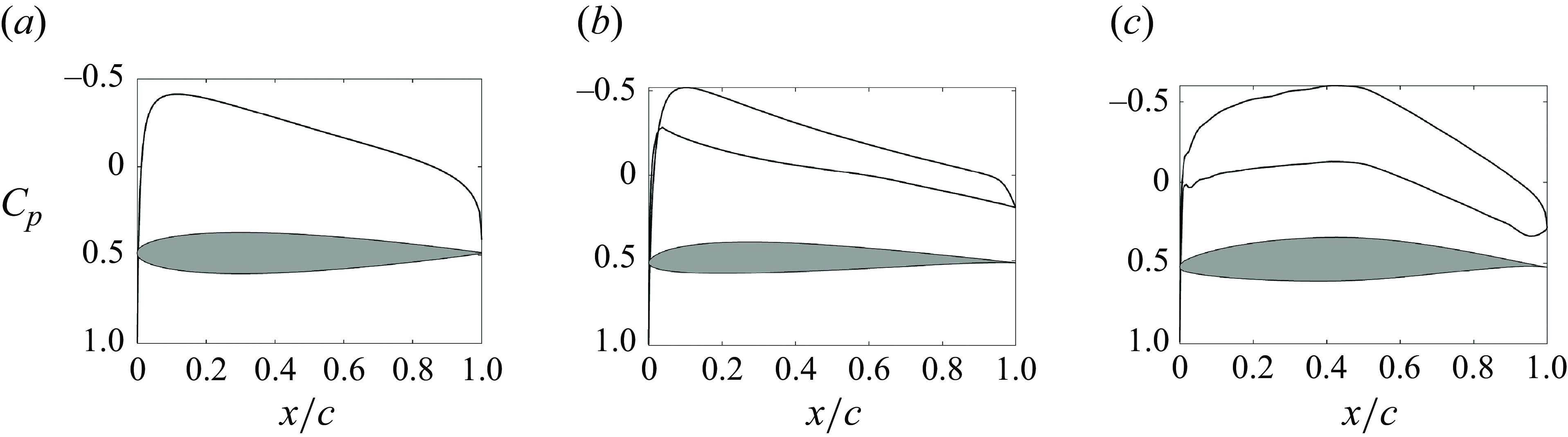
Figure 1. Pressure coefficients (black) for inviscid flow over airfoils (grey) at
 $\alpha = 0^{\circ }$
. NACA 0012 (a), SD 7003 (b) and NACA 65(1)–412 (c) (Drela Reference Drela and Mueller1989). The locations of maximum thickness are at
$\alpha = 0^{\circ }$
. NACA 0012 (a), SD 7003 (b) and NACA 65(1)–412 (c) (Drela Reference Drela and Mueller1989). The locations of maximum thickness are at
 $0.3c, 0.25c $
and 0.4c, respectively.
$0.3c, 0.25c $
and 0.4c, respectively.
1.4. Objectives
The goal of this paper is to provide a comprehensive and detailed description of the flow topology over a cambered NACA 65(1)–412 airfoil at
 $Re\,=\,2\times 10^4$
for
$Re\,=\,2\times 10^4$
for
 $\alpha$
from 0
$\alpha$
from 0
 $^{\circ }$
to 10
$^{\circ }$
to 10
 $^{\circ }$
through highly resolved DNS. At this specific Reynolds number, the flow is particularly sensitive to the transition dynamics and features entirely laminar states across the airfoil with a transitional wake, turbulent reattachment and the formation of separation bubbles of various sizes and locations within a narrow range of incidence angles. The simulations are conducted with a high-order, compressible, discontinuous Galerkin spectral element method (DGSEM) using a large span (0.5
$^{\circ }$
through highly resolved DNS. At this specific Reynolds number, the flow is particularly sensitive to the transition dynamics and features entirely laminar states across the airfoil with a transitional wake, turbulent reattachment and the formation of separation bubbles of various sizes and locations within a narrow range of incidence angles. The simulations are conducted with a high-order, compressible, discontinuous Galerkin spectral element method (DGSEM) using a large span (0.5
 $c$
) and large domain length and height (30
$c$
) and large domain length and height (30
 $c$
) to accurately capture the instabilities without altering the separation and transition dynamics through domain blockage. We set out to identify 3-D instabilities and show how they are connected to the formation of 3-D tubular structures and very large regions of turbulent coherence (‘puffs’). For selected
$c$
) to accurately capture the instabilities without altering the separation and transition dynamics through domain blockage. We set out to identify 3-D instabilities and show how they are connected to the formation of 3-D tubular structures and very large regions of turbulent coherence (‘puffs’). For selected
 $\alpha$
, we analyse the interaction of Kármán vortices, which originate from the pressure-side shear layer at the trailing edge of the airfoil, and the suction-side shear layer with its associated KH instabilities. It will be shown that 3-D instabilities of the near-wake region have an upstream influence on the evolution of the LSB and the complex dynamics of its time-averaged reattachment, for which there are significant improvements in performance, as measured by
$\alpha$
, we analyse the interaction of Kármán vortices, which originate from the pressure-side shear layer at the trailing edge of the airfoil, and the suction-side shear layer with its associated KH instabilities. It will be shown that 3-D instabilities of the near-wake region have an upstream influence on the evolution of the LSB and the complex dynamics of its time-averaged reattachment, for which there are significant improvements in performance, as measured by
 $L/D$
.
$L/D$
.
2. Computational formulation
2.1. Conservation laws
We compute solutions to the compressible Navier–Stokes equations, which can be written in non-dimensional form as
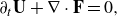 \begin{equation} \partial _t\mathbf {U} + \nabla \cdot \mathbf {F} = 0, \end{equation}
where
 $\mathbf {U}$
represents the vector of the conserved variables
$\mathbf {U}$
represents the vector of the conserved variables
 \begin{equation} \mathbf {U} = \left [\,\rho \quad \rho u \quad \rho v \quad \rho w \quad \rho e\,\right]^T, \end{equation}
where
 $\rho$
is the density and
$\rho$
is the density and
 $u$
,
$u$
,
 $v$
and
$v$
and
 $w$
are the velocity components. The specific total energy is
$w$
are the velocity components. The specific total energy is
 $\rho e\,=\,p/(\gamma -1)+({1}/{2})\rho (u^2+v^2+w^2)$
and the system is closed by the equation of state
$\rho e\,=\,p/(\gamma -1)+({1}/{2})\rho (u^2+v^2+w^2)$
and the system is closed by the equation of state
 \begin{equation} p = \frac {\rho T}{\gamma M_f^2}, \end{equation}
where
 $p$
,
$p$
,
 $T$
and
$T$
and
 $\gamma$
are the pressure, temperature and the ratio of specific heats, respectively, and
$\gamma$
are the pressure, temperature and the ratio of specific heats, respectively, and
 $M_f$
is the reference Mach number. The flux vector
$M_f$
is the reference Mach number. The flux vector
 $\mathbf {F}$
comprises an advective (superscript a) and a viscous part (superscript
$\mathbf {F}$
comprises an advective (superscript a) and a viscous part (superscript
 $v$
)
$v$
)
 \begin{equation} \nabla \cdot \mathbf {F} = \partial _x\mathbf {F}^a + \partial _y\mathbf {G}^a + \partial _z\mathbf {H}^a - \frac {1}{Re_f}\left (\partial _x\mathbf {F}^v + \partial _y\mathbf {G}^v + \partial _z\mathbf {H}^v\right), \end{equation}
where
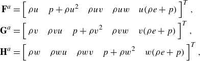 \begin{align} \mathbf {F}^a &= \left [\, \rho u \quad p + \rho u^2 \quad \rho u v \quad \rho u w \quad u(\rho e + p) \,\right]^T, \nonumber\\ \mathbf {G}^a &= \left [\, \rho v \quad \rho v u \quad p + \rho v^2 \quad \rho v w \quad v(\rho e + p) \,\right]^T, \nonumber\\ \mathbf {H}^a &= \left [\, \rho w \quad \rho w u \quad \rho w v \quad p + \rho w^2 \quad w(\rho e + p) \,\right]^T, \end{align}
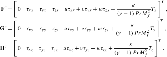 \begin{align} \mathbf {F}^v &= \left [\, 0 \quad \tau _{xx} \quad \tau _{yx} \quad \tau _{zx} \quad u \tau _{xx} + v \tau _{yx} + w \tau _{zx} + \frac {\kappa }{\left (\gamma -1\right)Pr M_f^2} T_x \,\right]^T, \nonumber\\ \mathbf {G}^v &= \left [\, 0 \quad \tau _{xy} \quad \tau _{yy} \quad \tau _{zy} \quad u \tau _{xy} + v \tau _{yy} + w \tau _{zy} + \frac {\kappa }{\left (\gamma -1\right)Pr M_f^2} T_y \,\right]^T, \nonumber\\ \mathbf {H}^v &= \left [\, 0 \quad \tau _{xz} \quad \tau _{yz} \quad \tau _{zz} \quad u \tau _{xz} + v \tau _{yz} + w \tau _{zz} + \frac {\kappa }{\left (\gamma -1\right)Pr M_f^2} T_z \,\right]^T. \end{align}
Here,
 $Re_f$
is the reference Reynolds number,
$Re_f$
is the reference Reynolds number,
 $Pr$
the Prandtl number and the stress tensor is
$Pr$
the Prandtl number and the stress tensor is
 $\tau _{ij}$
=
$\tau _{ij}$
=
 $2\mu (S_{ij}-S_{mm}\delta _{ij}/3)$
with the strain rate tensor
$2\mu (S_{ij}-S_{mm}\delta _{ij}/3)$
with the strain rate tensor
 $S_{ij}$
. The viscosity
$S_{ij}$
. The viscosity
 $\mu$
is calculated following Sutherland’s law
$\mu$
is calculated following Sutherland’s law
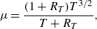 \begin{equation} \mu = \frac {(1+R_T)T^{3/2}}{T+R_T}, \end{equation}
where
 $R_T$
denotes the ratio of the Sutherland constant
$R_T$
denotes the ratio of the Sutherland constant
 $S$
to the reference temperature
$S$
to the reference temperature
 $T_f$
. All quantities are non-dimensionalised with respect to the airfoil chord length
$T_f$
. All quantities are non-dimensionalised with respect to the airfoil chord length
 $c$
, the free-stream velocity
$c$
, the free-stream velocity
 $U_\infty$
, density
$U_\infty$
, density
 $\rho _\infty$
and temperature
$\rho _\infty$
and temperature
 $T_\infty$
.
$T_\infty$
.
2.2. Boundary-layer relations
The boundary-layer velocity profile is extracted from DNS data according to the methods described by Alam & Sandham (Reference Alam and Sandham2000) and Uranga et al. (Reference Uranga, Persson, Drela and Peraire2011), who use a pseudo-velocity profile inside the rotational boundary-layer flow based on the spanwise vorticity
 \begin{equation} \mathbf {u}^*(s,\eta) = \int _0^\eta \mathbf {\boldsymbol {\omega }}(s,\tilde {\eta })\times \mathbf {n}(s)\,\mathrm {d}\tilde {\eta }, \end{equation}
where
 $s$
and
$s$
and
 $\eta$
refer to the wall-tangential and normal coordinates, respectively, and
$\eta$
refer to the wall-tangential and normal coordinates, respectively, and
 $\mathbf {n}(s)$
is the wall-normal unit vector. The boundary-layer edge
$\mathbf {n}(s)$
is the wall-normal unit vector. The boundary-layer edge
 $\eta _e$
is located at a distance where the vorticity magnitude and gradient are below a certain threshold and the flow is assumed to be irrotational (Uranga et al. Reference Uranga, Persson, Drela and Peraire2011). The displacement thickness
$\eta _e$
is located at a distance where the vorticity magnitude and gradient are below a certain threshold and the flow is assumed to be irrotational (Uranga et al. Reference Uranga, Persson, Drela and Peraire2011). The displacement thickness
 $\delta ^*$
and momentum thickness
$\delta ^*$
and momentum thickness
 $\theta$
are computed by integrating the velocity profile across the boundary layer
$\theta$
are computed by integrating the velocity profile across the boundary layer
 \begin{align} \delta ^*(s) &= \int _0^{\eta _e} \left (1-\frac {u_s(s,\eta)}{u_e(s)}\right)\mathrm {d}\eta, \end{align}
 \begin{align} \theta (s) &= \int _0^{\eta _e} \frac {u_s(s,\eta)}{u_e(s)}\left (1-\frac {u_s(s,\eta)}{u_e(s)}\right)\mathrm {d}\eta . \end{align}
Here,
 $u_s$
is the local, tangential velocity component and
$u_s$
is the local, tangential velocity component and
 $u_e$
the velocity magnitude evaluated at the boundary-layer edge
$u_e$
the velocity magnitude evaluated at the boundary-layer edge
 $\eta _e$
. The shape factor is defined as the ratio of displacement to momentum thickness,
$\eta _e$
. The shape factor is defined as the ratio of displacement to momentum thickness,
 $H$
=
$H$
=
 $\delta ^*/\theta$
.
$\delta ^*/\theta$
.
The exact locations of flow separation and reattachment are based on the zero crossings of the time- and space-averaged skin-friction coefficient according to theory by Haller (Reference Haller2004). In accordance with Uranga et al. (Reference Uranga, Persson, Drela and Peraire2011), the transition point indicates the location of a local maximum in the shape factor. We note, however, that the definition of the transition point is not unique; Alam & Sandham (Reference Alam and Sandham2000), for example, use the point of maximum negative skin friction.
3. Set-up
The flow over a cambered NACA 65(1)–412 airfoil is simulated in two and three dimensions at a chord-based Reynolds number of
 $Re_c$
=
$Re_c$
=
 $2\times 10^4$
and a free-stream Mach number of
$2\times 10^4$
and a free-stream Mach number of
 $M$
= 0.3. At this Mach number, the compressibility effect in terms of the pressure coefficient deviations are expected to be of the order of 5 % in relation to incompressible flow, according to the Prandtl–Glauert correction
$M$
= 0.3. At this Mach number, the compressibility effect in terms of the pressure coefficient deviations are expected to be of the order of 5 % in relation to incompressible flow, according to the Prandtl–Glauert correction
 $C_{p,M}/C_{p,i}$
=
$C_{p,M}/C_{p,i}$
=
 $1/\sqrt {1-M^2}$
. While the Mach number in comparable wind tunnel experiments is usually closer to 0.1, the stiffness of the explicitly time-integrated system of ordinary differential equations that remains after the spatial discretisation, results in time step sizes of the order of
$1/\sqrt {1-M^2}$
. While the Mach number in comparable wind tunnel experiments is usually closer to 0.1, the stiffness of the explicitly time-integrated system of ordinary differential equations that remains after the spatial discretisation, results in time step sizes of the order of
 $\mathcal {O}(10^{-6})$
that result in an excessive computational cost for 3-D simulations with only minor impact on the aerodynamics. Many of the incompressible results reported use this weakly compressible model to relax the time step restriction and to determine the nearly incompressible aerodynamics (Jones et al. Reference Jones, Sandberg and Sandham2008; Uranga et al. Reference Uranga, Persson, Drela and Peraire2011). The Prandtl number is set to
$\mathcal {O}(10^{-6})$
that result in an excessive computational cost for 3-D simulations with only minor impact on the aerodynamics. Many of the incompressible results reported use this weakly compressible model to relax the time step restriction and to determine the nearly incompressible aerodynamics (Jones et al. Reference Jones, Sandberg and Sandham2008; Uranga et al. Reference Uranga, Persson, Drela and Peraire2011). The Prandtl number is set to
 $Pr$
= 0.72. The Sutherland constant
$Pr$
= 0.72. The Sutherland constant
 $R_T$
=
$R_T$
=
 $S/T_f$
= 110/200 and ratio of specific heats
$S/T_f$
= 110/200 and ratio of specific heats
 $\gamma$
= 1.4 are chosen in accordance with Nelson (Reference Nelson2015).
$\gamma$
= 1.4 are chosen in accordance with Nelson (Reference Nelson2015).
The Navier–Stokes equations (2.1) are discretised with a DGSEM. The method and code are extensively discussed, tested and used for DNS in previous work (Kopriva Reference Kopriva2009; Klose, Jacobs & Kopriva Reference Klose, Jacobs and Kopriva2020 and references therein). The DGSEM approximates the conservative variables (2.2) spatially through a Nth-order polynomial basis (collocated on quadrature nodes of Legendre polynomials) and on non-overlapping elements. The elements are connected weakly and conservatively on the fluxes. The Roe scheme is used to determine the advective interface fluxes and a Bassi–Rebay formulation determines the viscous fluxes. A fourth-order explicit Runge–Kutta scheme is used for time integration. Time step sizes are in the range
 $2.3\times 10^{-5}$
 $\leqslant$
 $\Delta t$
 $\leqslant$
 $8.4\times 10^{-6}$
, depending on the element size and the polynomial order.
$8.4\times 10^{-6}$
, depending on the element size and the polynomial order.
Free-stream conditions are enforced weakly on the fluxes at the outer boundaries of the domain using approximate Riemann solvers. Spurious oscillations from exiting vortices are decreased through grid coarsening towards the outflow, as well as a damping layer on the energy term to reduce the reflected pressure waves (Jacobs, Kopriva & Mashayek Reference Jacobs, Kopriva and Mashayek2003). The surface of the airfoil is treated as no-slip adiabatic wall and, to account for its curvature, we fit the neighbouring boundary elements to a spline representing the profile of the airfoil according to Nelson, Jacobs & Kopriva (Reference Nelson, Jacobs and Kopriva2016). For 3-D simulations, the mesh is extruded in the spanwise direction and the boundaries are set to be periodic to model an infinite wing.
The simulations are run until the flow has fully transitioned to a 3-D state and the solution has reached quasi-steady state with the lift and drag coefficients fluctuating around a mean. Flow statistics are recorded subsequently, with the integration times given in table 2.
3.1. Domain size
The size of the computational domain can affect the numerical solution through blockage and spurious reflections from the outer boundaries. A compromise has to be made between a domain large enough to minimise such boundary effects and the available computational resources that necessarily limit the number of grid points.
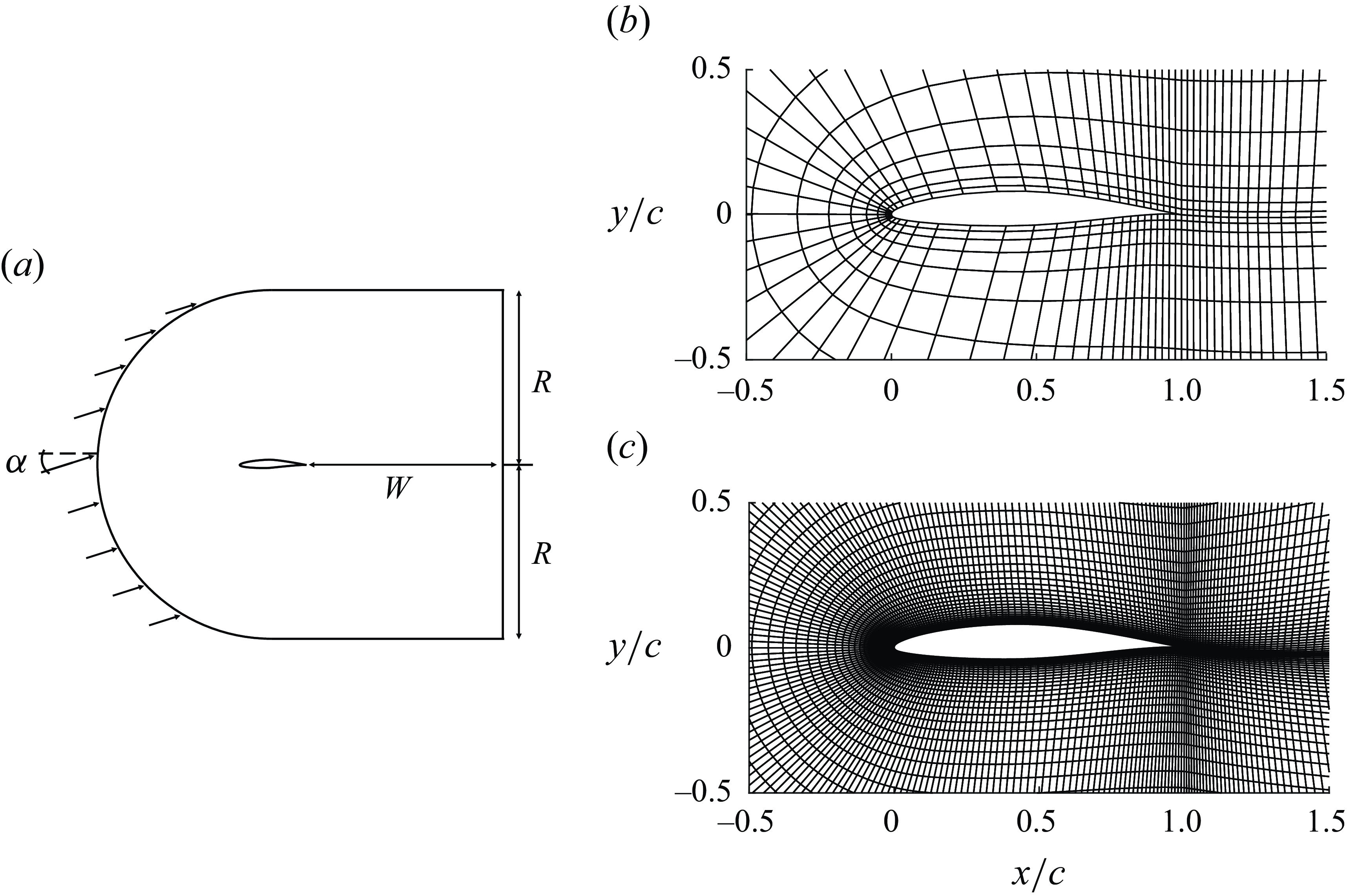
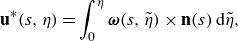
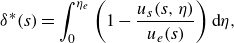
Figure 2. (a) A C-type computational domain with general parameters. Elements of 2-D computational meshes for grid 1 (b) and grid 2 (c) around the airfoil. Only elements without interior Gauss nodes are shown.
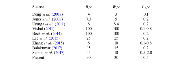
For the C-type computational domain that is used and schematically shown in figure 2, the domain size is defined entirely by the radius R and the wake length W, which are both set to
 $30\textit {c}$
. This value is greater than in most comparable studies, as collated in table 1, that report on domain radii ranging from 4c (Deng, Jiang & Liu Reference Deng, Jiang and Liu2007) to 100c (Visbal Reference Visbal2011; Beck et al. Reference Beck, Bolemann, Flad, Frank, Gassner, Hindenlang and Munz2014) and wake lengths from 3c to 100c. The large domain size was found to be necessary to minimise spurious reflections from the outflow boundaries or changes in the separation bubble shape (Beck et al. Reference Beck, Bolemann, Flad, Frank, Gassner, Hindenlang and Munz2014). The C-mesh is extruded in the
$30\textit {c}$
. This value is greater than in most comparable studies, as collated in table 1, that report on domain radii ranging from 4c (Deng, Jiang & Liu Reference Deng, Jiang and Liu2007) to 100c (Visbal Reference Visbal2011; Beck et al. Reference Beck, Bolemann, Flad, Frank, Gassner, Hindenlang and Munz2014) and wake lengths from 3c to 100c. The large domain size was found to be necessary to minimise spurious reflections from the outflow boundaries or changes in the separation bubble shape (Beck et al. Reference Beck, Bolemann, Flad, Frank, Gassner, Hindenlang and Munz2014). The C-mesh is extruded in the
 $z$
-direction by
$z$
-direction by
 $L_z$
= 0.5
$L_z$
= 0.5
 $c$
, following the recommendations by Almutairi et al. (Reference Almutairi, Jones and Sandham2010) in their LES of the NACA 0012 airfoil aerodynamics with periodic boundary conditions in the spanwise direction.
$c$
, following the recommendations by Almutairi et al. (Reference Almutairi, Jones and Sandham2010) in their LES of the NACA 0012 airfoil aerodynamics with periodic boundary conditions in the spanwise direction.
Table 1. Domain sizes of selected airfoil studies.
3.2. Direct numerical simulation resolution
For a numerical Navier–Stokes solution to be called a DNS, i.e. a true solution to the Navier–Stokes equations, all relevant scales need to be resolved by the numerical discretisation. In marginally grid-resolved and under-resolved Navier–Stokes solutions, the subgrid-scale stresses may be implicitly modelled through the inherent dissipation of a numerical scheme (implicit LES (Grinstein, Margolin & Rider Reference Grinstein, Margolin and Rider2007; de Wiart et al. Reference de Wiart, Hillewaert, Bricteux and Winckelmans2015)) or explicitly modelled by a numerical filter (explicitly filtered LES, or EFLES (Gassner & Beck Reference Gassner and Beck2013; Ghiasi et al. Reference Ghiasi, Komperda, Li, Peyvan, Nicholls and Mashayek2019)). The inherent numerical dissipation and dispersion characteristics determine the deviation of a marginally resolved Navier–Stokes solution from DNS. The numerical dissipation is closely related to the dispersion relation, which varies per numerical scheme, and can be assessed through numerical analysis Gassner & Kopriva (Reference Gassner and Kopriva2011). High-order spectral methods have a distinct advantage over lower-order finite volume or finite difference schemes as they require far fewer points per wavelength to resolve a flow feature and by concentrating the dissipation at the highest wavenumbers (Gassner & Kopriva Reference Gassner and Kopriva2011; de Wiart et al. Reference Carton de Wiart, Hillewaert, Duponcheel and Winckelmans2014). Jacobs, Kopriva & Mashayek (Reference Jacobs, Kopriva and Mashayek2005), for example, showed that a spectral element method with polynomial order of
 $N$
= 13 requires only 3 points per wave.
$N$
= 13 requires only 3 points per wave.
The grid independency of the numerical solution for the large computational domain is assessed by comparing simulation results for two C-meshes that are based upon the known grid-resolved meshes for smaller computational domains from previous studies. The two meshes include grid 1 consisting of 3 366 quadrilateral elements in the x-y plane, which is extruded by 10 elements along the span for 3-D simulations (see figure 2
b) and grid 2, which is refined by 23 400 elements in the
 $x$
-
$x$
-
 $y$
plane and by 50 elements in spanwise direction (see figure 2
c). In Klose et al. (Reference Klose, Jacobs and Kopriva2020), we assessed the impact of underresolution for the DGSEM and showed that the kinetic-energy-preserving formulation of the method predicts Navier–Stokes solutions for the NACA 65–412 at
$y$
plane and by 50 elements in spanwise direction (see figure 2
c). In Klose et al. (Reference Klose, Jacobs and Kopriva2020), we assessed the impact of underresolution for the DGSEM and showed that the kinetic-energy-preserving formulation of the method predicts Navier–Stokes solutions for the NACA 65–412 at
 $\alpha$
= 4
$\alpha$
= 4
 $^{\circ }$
well at a marginal resolution within 2 %.
$^{\circ }$
well at a marginal resolution within 2 %.
At angles of attack
 $\alpha$
< 6
$\alpha$
< 6
 $^{\circ }$
, the flow is characterised by a laminar separation, and instabilities occur downstream of the airfoil in the wake area. Commensurate with this flow characterisation, a coarse grid and a high-order approximation suffice for a grid-resolved solution up to the wake. In the near wake, where nonlinear instabilities eventually lead to a transition to turbulence, the normalised element size (i.e. divided by
$^{\circ }$
, the flow is characterised by a laminar separation, and instabilities occur downstream of the airfoil in the wake area. Commensurate with this flow characterisation, a coarse grid and a high-order approximation suffice for a grid-resolved solution up to the wake. In the near wake, where nonlinear instabilities eventually lead to a transition to turbulence, the normalised element size (i.e. divided by
 $N$
+ 1) is approximately
$N$
+ 1) is approximately
 $\leqslant 3.8\eta$
, where
$\leqslant 3.8\eta$
, where
 $\eta$
is the Kolmogorov scale
$\eta$
is the Kolmogorov scale
 $\eta \,=\,(\nu ^3 / \varepsilon)^{{1}/{4}}$
and
$\eta \,=\,(\nu ^3 / \varepsilon)^{{1}/{4}}$
and
 $\varepsilon$
the dissipation of the turbulent kinetic energy. This value is taken at the location of maximum dissipation
$\varepsilon$
the dissipation of the turbulent kinetic energy. This value is taken at the location of maximum dissipation
 $\varepsilon$
(just downstream of the trailing edge with
$\varepsilon$
(just downstream of the trailing edge with
 $\eta /c$
= 0.001), which is computed from the time-averaged flow field. This is well within the reported requirement for the ratio of the smallest grid spacing to the Kolmogorov scale,
$\eta /c$
= 0.001), which is computed from the time-averaged flow field. This is well within the reported requirement for the ratio of the smallest grid spacing to the Kolmogorov scale,
 $\Delta x/\eta$
 $\leqslant$
12, to resolve the peak dissipation or
$\leqslant$
12, to resolve the peak dissipation or
 $\Delta x/\eta$
 $\leqslant$
4 to resolve the bulk of the turbulent dissipation (Pope Reference Pope2000; Fröhlich et al. Reference Fröhlich, Mellen, Rodi, Temmerman and Leschziner2005), which assumes that two points are required to resolve a flow feature. We also note that the grid spacing estimate based on the normalisation with the polynomial order
$\leqslant$
4 to resolve the bulk of the turbulent dissipation (Pope Reference Pope2000; Fröhlich et al. Reference Fröhlich, Mellen, Rodi, Temmerman and Leschziner2005), which assumes that two points are required to resolve a flow feature. We also note that the grid spacing estimate based on the normalisation with the polynomial order
 $N$
is a conservative estimate given that at high polynomial orders significantly fewer grid points are necessary to resolve a wave compared with lower-order schemes. For
$N$
is a conservative estimate given that at high polynomial orders significantly fewer grid points are necessary to resolve a wave compared with lower-order schemes. For
 $Re\,=\,2\times 10^4$
and
$Re\,=\,2\times 10^4$
and
 $\alpha$
= 4
$\alpha$
= 4
 $^{\circ }$
, Nelson et al. (Reference Nelson, Jacobs and Kopriva2016) and Klose et al. (Reference Klose, Jacobs and Kopriva2020) have reported a grid-converged solution at a polynomial of
$^{\circ }$
, Nelson et al. (Reference Nelson, Jacobs and Kopriva2016) and Klose et al. (Reference Klose, Jacobs and Kopriva2020) have reported a grid-converged solution at a polynomial of
 $N$
= 12 for a mesh nearly identical to grid 1, but limited to
$N$
= 12 for a mesh nearly identical to grid 1, but limited to
 $R$
= 5
$R$
= 5
 $c$
and
$c$
and
 $W$
= 15
$W$
= 15
 $c$
. Klose et al. (Reference Klose, Jacobs and Kopriva2020) show that to prevent numerical instabilities related to marginal resolution at
$c$
. Klose et al. (Reference Klose, Jacobs and Kopriva2020) show that to prevent numerical instabilities related to marginal resolution at
 $\alpha$
= 10
$\alpha$
= 10
 $^{\circ }$
, the kinetic energy conserving formulation is required as it enhances numerical stability of DGSEM. While the coarse grid is grid converged at
$^{\circ }$
, the kinetic energy conserving formulation is required as it enhances numerical stability of DGSEM. While the coarse grid is grid converged at
 $N$
= 12 for the smooth flows at lower angles of attack (
$N$
= 12 for the smooth flows at lower angles of attack (
 $\alpha$
= 0
$\alpha$
= 0
 $^{\circ }$
, 4
$^{\circ }$
, 4
 $^{\circ }$
), the refined grid 2 with lower orders of
$^{\circ }$
), the refined grid 2 with lower orders of
 $N$
= 4–6 for computations is used at higher
$N$
= 4–6 for computations is used at higher
 $\alpha$
= 6
$\alpha$
= 6
 $^{\circ }$
, 7
$^{\circ }$
, 7
 $^{\circ }$
and 8
$^{\circ }$
and 8
 $^{\circ }$
, because the flow instabilities occur upstream of the trailing edge and an increased near-wall resolution of the fine grid adds resolution in the boundary-layer region. This is more suited to wall-bounded turbulent flow and the accompanying increase in wall shear stress. At
$^{\circ }$
, because the flow instabilities occur upstream of the trailing edge and an increased near-wall resolution of the fine grid adds resolution in the boundary-layer region. This is more suited to wall-bounded turbulent flow and the accompanying increase in wall shear stress. At
 $\alpha$
= 6
$\alpha$
= 6
 $^{\circ }$
, the flow is still laminar over the entire airfoil and transition occurs along the separated shear layer and within the near wake at the trailing edge. Here, the normalised grid spacing does not exceed
$^{\circ }$
, the flow is still laminar over the entire airfoil and transition occurs along the separated shear layer and within the near wake at the trailing edge. Here, the normalised grid spacing does not exceed
 $2.2\eta$
. At
$2.2\eta$
. At
 $\alpha$
= 7
$\alpha$
= 7
 $^{\circ }$
, the normalised non-dimensional cell spacings at the turbulent transition peak (
$^{\circ }$
, the normalised non-dimensional cell spacings at the turbulent transition peak (
 $x/c$
= 0.7) in the streamwise, wall-normal and spanwise directions are
$x/c$
= 0.7) in the streamwise, wall-normal and spanwise directions are
 $\xi ^+$
= 10,
$\xi ^+$
= 10,
 $\eta ^+$
< 1,
$\eta ^+$
< 1,
 $\zeta ^+$
= 5. The normalised grid spacing at the dissipation peak above the wall (
$\zeta ^+$
= 5. The normalised grid spacing at the dissipation peak above the wall (
 $x/c$
= 0.7,
$x/c$
= 0.7,
 $\eta /c$
= 0.0008) is
$\eta /c$
= 0.0008) is
 $\Delta x/\eta$
 $\approx$
4.0. For
$\approx$
4.0. For
 $\alpha$
= 8
$\alpha$
= 8
 $^{\circ }$
, the normalised non-dimensional cell spacings at the turbulent transition peak (
$^{\circ }$
, the normalised non-dimensional cell spacings at the turbulent transition peak (
 $x/c$
= 0.4) are
$x/c$
= 0.4) are
 $\xi ^+$
= 8,
$\xi ^+$
= 8,
 $\eta ^+$
< 1,
$\eta ^+$
< 1,
 $\zeta ^+$
= 4. These values are well within the limits accepted for wall-resolved DNS (Georgiadis, Rizzetta & Fureby Reference Georgiadis, Rizzetta and Fureby2010). The normalised grid spacing at the dissipation peak above the wall (
$\zeta ^+$
= 4. These values are well within the limits accepted for wall-resolved DNS (Georgiadis, Rizzetta & Fureby Reference Georgiadis, Rizzetta and Fureby2010). The normalised grid spacing at the dissipation peak above the wall (
 $x/c$
= 0.4,
$x/c$
= 0.4,
 $\eta /c$
= 0.0007) is
$\eta /c$
= 0.0007) is
 $\Delta x/\eta$
 $\approx$
4.7. While this value is slightly above 4, we note that for
$\approx$
4.7. While this value is slightly above 4, we note that for
 $\alpha$
= 8
$\alpha$
= 8
 $^{\circ }$
we use a polynomial order of
$^{\circ }$
we use a polynomial order of
 $N$
= 6, which yields a seventh-order accurate scheme in space and hence allows for fewer grid points per wavelength.
$N$
= 6, which yields a seventh-order accurate scheme in space and hence allows for fewer grid points per wavelength.
For
 $\alpha$
= 10
$\alpha$
= 10
 $^{\circ }$
, the smallest scales of turbulence are marginally resolved, and the kinetic energy preserving scheme has to be employed. Because the flow is past the critical transition angle (7
$^{\circ }$
, the smallest scales of turbulence are marginally resolved, and the kinetic energy preserving scheme has to be employed. Because the flow is past the critical transition angle (7
 $^{\circ }$
–8
$^{\circ }$
–8
 $^{\circ }$
), a computationally more efficient set-up resolves the flow on grid 1 with twelfth-order polynomials in the near field, with reduced order elements in the outer field. A weak spectral filter reduces spurious oscillations arising from the decreasing order (p-coarsening) away from the airfoil. It is not appropriate to classify this simulation as DNS, and EFLES is more appropriate.
$^{\circ }$
), a computationally more efficient set-up resolves the flow on grid 1 with twelfth-order polynomials in the near field, with reduced order elements in the outer field. A weak spectral filter reduces spurious oscillations arising from the decreasing order (p-coarsening) away from the airfoil. It is not appropriate to classify this simulation as DNS, and EFLES is more appropriate.
The test matrix of 3-D simulations is collated in table 2 for different meshes, polynomial orders and refinements.
Table 2. Overview of 3-D simulations. Here,
 $Re$
= free-stream Reynolds number,
$Re$
= free-stream Reynolds number,
 $\alpha$
= angle of attack,
$\alpha$
= angle of attack,
 $R/c$
= domain radius, G = standard Gauss DGSEM (* = with spectral filter), GL-SF = split form DGSEM with Gauss–Lobatto nodes,
$R/c$
= domain radius, G = standard Gauss DGSEM (* = with spectral filter), GL-SF = split form DGSEM with Gauss–Lobatto nodes,
 $T_{init}$
/
$T_{init}$
/
 $T_{fin}$
= initial/final convective time of run,
$T_{fin}$
= initial/final convective time of run,
 $^a$
= initialised with uniform velocity field,
$^a$
= initialised with uniform velocity field,
 $^b$
= initialised with 2-D result,
$^b$
= initialised with 2-D result,
 $T_{stat}$
= integration time of statistics, (2x) = h-refined,
$T_{stat}$
= integration time of statistics, (2x) = h-refined,
 $N_i$
(
$N_i$
(
 $N_o$
) = polynomial order inner (outer) region, DOF = degrees of freedom (number of high-order nodes).
$N_o$
) = polynomial order inner (outer) region, DOF = degrees of freedom (number of high-order nodes).

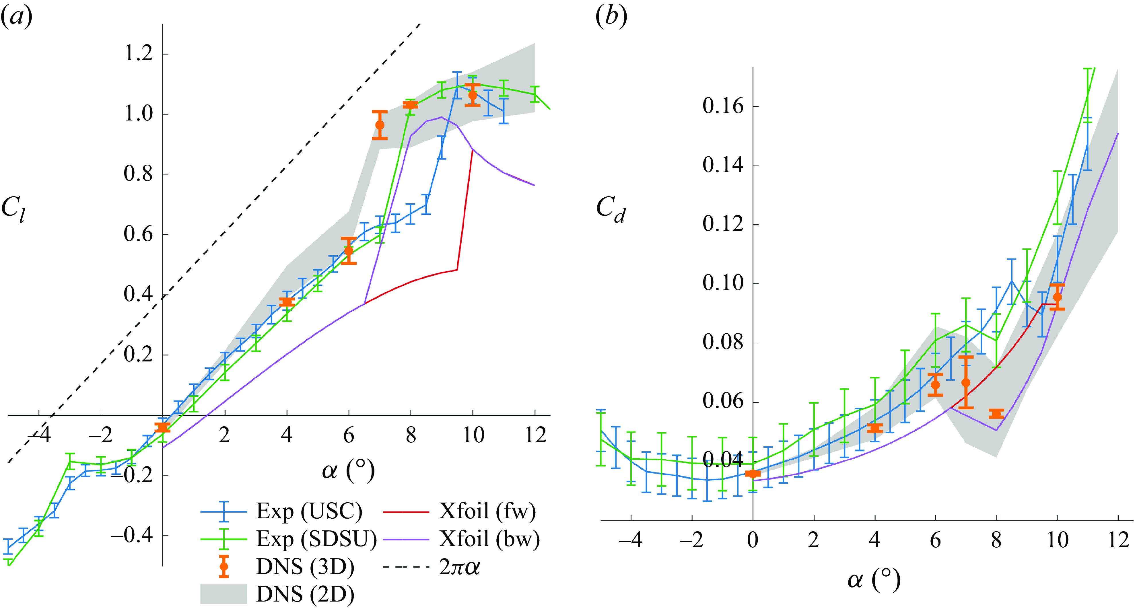
Figure 3. Lift (a) and drag (b) coefficients obtained from wind tunnel experiments at The University of Southern California (USC) and San Diego State University (SDSU), DNS data (two- and three-dimensional) and Xfoil data (forward and backward sweep,
 $N_{\textit{crit}}=9$
) for a NACA 65(1)–412 at
$N_{\textit{crit}}=9$
) for a NACA 65(1)–412 at
 $Re_c$
= 2
$Re_c$
= 2
 $\times 10^4$
. Error bars come from standard deviation of DNS time series and the grey area identifies the total lift and drag range of the parametric 2-D study given by the averaged coefficient +/- standard deviation. The error bars in experiments come from the standard deviation of time averages obtained from separate, repeated experiments.
$\times 10^4$
. Error bars come from standard deviation of DNS time series and the grey area identifies the total lift and drag range of the parametric 2-D study given by the averaged coefficient +/- standard deviation. The error bars in experiments come from the standard deviation of time averages obtained from separate, repeated experiments.
4. Results and discussion
4.1. A time-averaged view of the forces and flow fields
4.1.1. Integrated forces on the foil
Figure 3 compiles data from 3-D and 2-D DNS together with measurements from two different wind tunnel experiments (Choi Reference Choi2020; Tank et al. Reference Tank, Klose, Jacobs and Spedding2021). Also included are calculations from the panel code Xfoil (Drela Reference Drela and Mueller1989) which uses a boundary integral method to estimate separation locations. In Xfoil a tuneable parameter,
 $N_{\textit{crit}}$
sets a transition threshold. It is set to its default value of 9.
$N_{\textit{crit}}$
sets a transition threshold. It is set to its default value of 9.
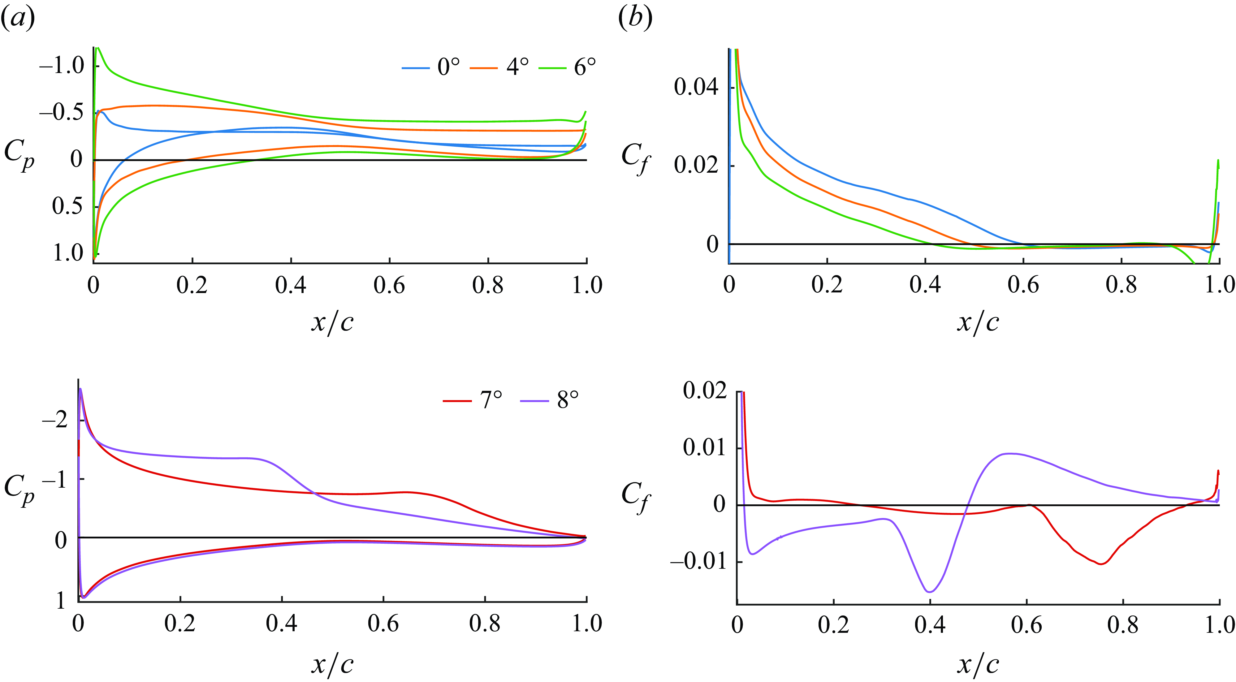
Figure 4. Time- and spanwise-averaged pressure (upper and lower side) and skin-friction (upper side) coefficients for
 $\alpha$
= 0
$\alpha$
= 0
 $^{\circ }$
, 4
$^{\circ }$
, 4
 $^{\circ }$
, 6
$^{\circ }$
, 6
 $^{\circ }$
(top row), 7
$^{\circ }$
(top row), 7
 $^{\circ }$
, and 8
$^{\circ }$
, and 8
 $^{\circ }$
(bottom row).
$^{\circ }$
(bottom row).
All computations and experiments show a sudden and significant increase in
 $C_l$
at a critical angle of attack,
$C_l$
at a critical angle of attack,
 $\alpha _{\textit{crit}}$
. The 3-D DNS result shows that
$\alpha _{\textit{crit}}$
. The 3-D DNS result shows that
 $C_l$
nearly doubles at
$C_l$
nearly doubles at
 $\alpha _{\textit{crit}}=7^{\circ }$
. The increases in
$\alpha _{\textit{crit}}=7^{\circ }$
. The increases in
 $C_l$
is accompanied by a decrease in
$C_l$
is accompanied by a decrease in
 $C_d$
. These changes in forcings coefficients are associated with an intricate interaction between 2-D and 3-D instabilities in the shear layer that develops in the lee of what may now be termed a closed LSB. These interactions will be discussed in detail below.
$C_d$
. These changes in forcings coefficients are associated with an intricate interaction between 2-D and 3-D instabilities in the shear layer that develops in the lee of what may now be termed a closed LSB. These interactions will be discussed in detail below.
For
 $\alpha \lt \alpha _{\textit{crit}}$
, experiments and 3-D DNS follow the same nonlinear curve of
$\alpha \lt \alpha _{\textit{crit}}$
, experiments and 3-D DNS follow the same nonlinear curve of
 $C_l(\alpha)$
. The 2-D DNS values occupy an envelope lying above the experiment-DNS line. At
$C_l(\alpha)$
. The 2-D DNS values occupy an envelope lying above the experiment-DNS line. At
 $\alpha _{\textit{crit}}$
, both 2-D and 3-D DNS rise at the same point. Experiments follow after, either at
$\alpha _{\textit{crit}}$
, both 2-D and 3-D DNS rise at the same point. Experiments follow after, either at
 $\alpha = 8^{\circ }$
(UCSD) or at
$\alpha = 8^{\circ }$
(UCSD) or at
 $9^{\circ }$
(USC). Once
$9^{\circ }$
(USC). Once
 $\alpha _{\textit{crit}}$
has been reached, the peak
$\alpha _{\textit{crit}}$
has been reached, the peak
 $C_l$
estimates are within uncertainties.
$C_l$
estimates are within uncertainties.
There is a larger variation in
 $C_d$
, in all estimates, particularly close to
$C_d$
, in all estimates, particularly close to
 $\alpha _{\textit{crit}}$
, but the various estimates do not differ beyond uncertainty. Both 3-D DNS and the SDSU data show a drop in
$\alpha _{\textit{crit}}$
, but the various estimates do not differ beyond uncertainty. Both 3-D DNS and the SDSU data show a drop in
 $C_d$
at
$C_d$
at
 $\alpha = 8^{\circ }$
, which is beyond
$\alpha = 8^{\circ }$
, which is beyond
 $\alpha _{\textit{crit}}$
in the DNS.
$\alpha _{\textit{crit}}$
in the DNS.
It is remarkable that the inviscid panel code Xfoil shares all the basic features of figure 3. Xfoil uses a boundary-layer model to include viscous effects, and then transition at some
 $N_{\textit{crit}}$
. The boundary-layer dynamics is always strongly influential at such low
$N_{\textit{crit}}$
. The boundary-layer dynamics is always strongly influential at such low
 $Re_c$
. The consistently lower
$Re_c$
. The consistently lower
 $C_l$
from Xfoil arises because the unsteady motions close to the trailing edge affect the upstream curvature of the laminar boundary layer. As a reference and reminder of how far away we are from design
$C_l$
from Xfoil arises because the unsteady motions close to the trailing edge affect the upstream curvature of the laminar boundary layer. As a reference and reminder of how far away we are from design
 $Re_c$
, the thin airfoil
$Re_c$
, the thin airfoil
 $C_l = 2\pi \alpha$
curve is shown with
$C_l = 2\pi \alpha$
curve is shown with
 $C_l = 0.4$
at
$C_l = 0.4$
at
 $\alpha = 0^{\circ }$
. Here, at
$\alpha = 0^{\circ }$
. Here, at
 $\alpha = 0^{\circ }$
,
$\alpha = 0^{\circ }$
,
 $C_l \lt 0$
.
$C_l \lt 0$
.
The time-averaged profiles of the pressure and skin-friction coefficients for
 $\alpha$
= 0
$\alpha$
= 0
 $^{\circ }$
, 4
$^{\circ }$
, 4
 $^{\circ }$
, 6
$^{\circ }$
, 6
 $^{\circ }$
, 7
$^{\circ }$
, 7
 $^{\circ }$
and 8
$^{\circ }$
and 8
 $^{\circ }$
are shown in figure 4. At lower angles (
$^{\circ }$
are shown in figure 4. At lower angles (
 $\alpha$
 $\leqslant$
6
$\leqslant$
6
 $^{\circ }$
), the suction peak and the resulting adverse pressure gradient are small and the skin-friction coefficient gradually decreases until it becomes negative at the fixed separation point, as identified at the time-averaged zero-skin-friction point in Haller (Reference Haller2004), at
$^{\circ }$
), the suction peak and the resulting adverse pressure gradient are small and the skin-friction coefficient gradually decreases until it becomes negative at the fixed separation point, as identified at the time-averaged zero-skin-friction point in Haller (Reference Haller2004), at
 $x_{s,0^{\circ }}$
= 0.6 and
$x_{s,0^{\circ }}$
= 0.6 and
 $x_{s,4^{\circ }}$
= 0.49 (figure 4
b). Downstream of the separation location, the surface pressure remains constant and does not recover the free-stream value at the trailing edge. At higher
$x_{s,4^{\circ }}$
= 0.49 (figure 4
b). Downstream of the separation location, the surface pressure remains constant and does not recover the free-stream value at the trailing edge. At higher
 $\alpha$
 $\geqslant$
7
$\geqslant$
7
 $^{\circ }$
, the suction peak increases from
$^{\circ }$
, the suction peak increases from
 $C_p$
= −0.6 at
$C_p$
= −0.6 at
 $\alpha$
= 4
$\alpha$
= 4
 $^{\circ }$
to
$^{\circ }$
to
 $C_p$
= −2.5 at 7
$C_p$
= −2.5 at 7
 $^{\circ }$
and 8
$^{\circ }$
and 8
 $^{\circ }$
and steepens the adverse pressure gradient and promotes flow separation further upstream at
$^{\circ }$
and steepens the adverse pressure gradient and promotes flow separation further upstream at
 $x_{s,7^{\circ }}$
= 0.26 and
$x_{s,7^{\circ }}$
= 0.26 and
 $x_{s,8^{\circ }}$
= 0.02. The skin-friction coefficient at 8
$x_{s,8^{\circ }}$
= 0.02. The skin-friction coefficient at 8
 $^{\circ }$
shows a shape typical for LSBs (cf. Jones et al. Reference Jones, Sandberg and Sandham2008) with a pronounced negative peak around the transition point. At
$^{\circ }$
shows a shape typical for LSBs (cf. Jones et al. Reference Jones, Sandberg and Sandham2008) with a pronounced negative peak around the transition point. At
 $\alpha$
= 7
$\alpha$
= 7
 $^{\circ }$
, the LSB is located at the trailing edge and the skin-friction profile indicates that the wall shear stress remains near zero over two thirds of the airfoil until the flow transitions at
$^{\circ }$
, the LSB is located at the trailing edge and the skin-friction profile indicates that the wall shear stress remains near zero over two thirds of the airfoil until the flow transitions at
 $x_{t,7^{\circ }}/c$
= 0.62 and transports momentum to the surface that results in a peak of the shear stress at
$x_{t,7^{\circ }}/c$
= 0.62 and transports momentum to the surface that results in a peak of the shear stress at
 $x/c$
= 0.75.
$x/c$
= 0.75.
4.1.2. The time-averaged flow field
A comparison of the time- and space-averaged streamline patterns in figure 5 demonstrates the change in flow topology from a region of separated, recirculating flow at the trailing edge into a LSB and its swift shift (within one degree
 $\alpha$
) towards the leading edge. Because the maximum height of the airfoil is at
$\alpha$
) towards the leading edge. Because the maximum height of the airfoil is at
 $x/c$
= 0.4, the LSB is either formed upstream or downstream of that point and not at mid-chord.
$x/c$
= 0.4, the LSB is either formed upstream or downstream of that point and not at mid-chord.
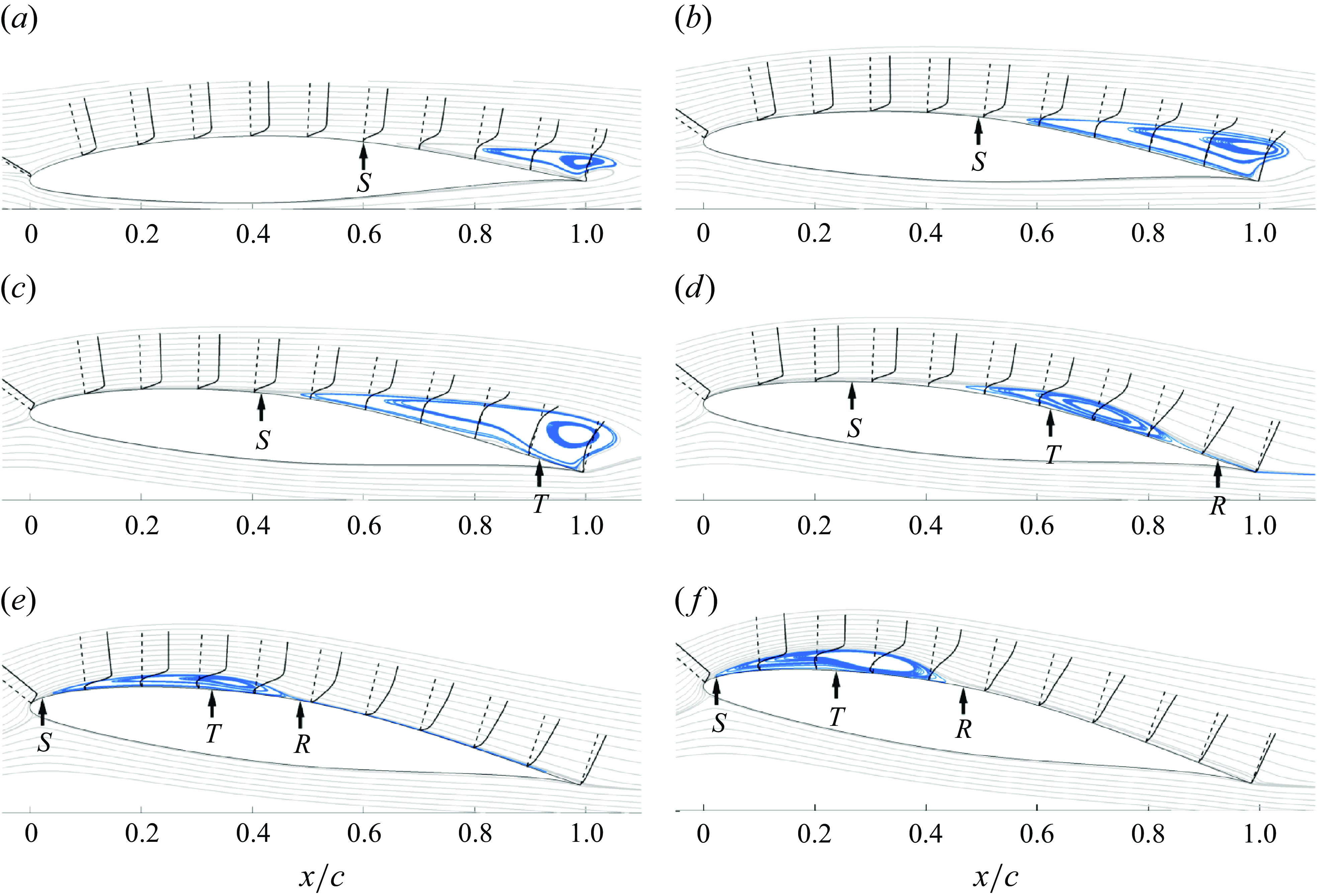
Figure 5. Time- and space-averaged streamlines for
 $\alpha$
from 0
$\alpha$
from 0
 $^{\circ }$
(a) to 10
$^{\circ }$
(a) to 10
 $^{\circ }$
(f). Recirculating flow in blue. Here, S, T and R indicate the mean locations of separation, transition and reattachment.
$^{\circ }$
(f). Recirculating flow in blue. Here, S, T and R indicate the mean locations of separation, transition and reattachment.
In general, three regimes may be identified from figure 5. In the low-
 $\alpha$
regime there is laminar separation without reattachment. The large recirculating zone increases in size with low-speed fluid attached to an increasingly large extent of the suction surface. The outer flow streamlines do not follow the airfoil contour but trace the outline of the separated region. The separated region closes only aft of the trailing edge. This low-
$\alpha$
regime there is laminar separation without reattachment. The large recirculating zone increases in size with low-speed fluid attached to an increasingly large extent of the suction surface. The outer flow streamlines do not follow the airfoil contour but trace the outline of the separated region. The separated region closes only aft of the trailing edge. This low-
 $\alpha$
regime has been termed SI by Yang & Spedding (Reference Yang and Spedding2013a
), as one of two stable states (the other being SII at high
$\alpha$
regime has been termed SI by Yang & Spedding (Reference Yang and Spedding2013a
), as one of two stable states (the other being SII at high
 $\alpha$
), with a sharp transient regime between.
$\alpha$
), with a sharp transient regime between.
At
 $\alpha _{\textit{crit}}$
, the separated region suddenly collapses as the separation point moves upstream and transition occurs before reattachment just before the trailing edge. The outer flow streamlines also meet before the trailing edge and the effective airfoil shape (geometry plus boundary-layer displacement thickness) is one with increased camber. These transitions are responsible for the jump in
$\alpha _{\textit{crit}}$
, the separated region suddenly collapses as the separation point moves upstream and transition occurs before reattachment just before the trailing edge. The outer flow streamlines also meet before the trailing edge and the effective airfoil shape (geometry plus boundary-layer displacement thickness) is one with increased camber. These transitions are responsible for the jump in
 $C_l$
and decrease in
$C_l$
and decrease in
 $C_d$
. In this time-averaged view, the LSB has a positive effect, increasing lift and decreasing drag.
$C_d$
. In this time-averaged view, the LSB has a positive effect, increasing lift and decreasing drag.
In the third stage (high-
 $\alpha$
, or SII), the separation point has moved to just behind the leading edge, transition occurs before mid-chord, and the flow reattaches to form a thin bubble, which gradually grows in thickness with increasing
$\alpha$
, or SII), the separation point has moved to just behind the leading edge, transition occurs before mid-chord, and the flow reattaches to form a thin bubble, which gradually grows in thickness with increasing
 $\alpha$
, while shrinking in
$\alpha$
, while shrinking in
 $x$
.
$x$
.
This kind of development of a LSB is quite well-known in the literature (e.g. Galbraith & Visbal Reference Galbraith and Visbal2010), although its effect on
 $C_l$
and
$C_l$
and
 $C_d$
is not so clear as it depends on
$C_d$
is not so clear as it depends on
 $Re$
. The account is self-consistent and describes the phenomenology satisfactorily. However, the mechanisms for these various flow transitions are not necessarily evident, and in practice, the flow over the airfoil and in the near wake is always unsteady and three-dimensional. It is the purpose of the remainder of the paper to investigate the complex flows that are responsible for the simplified picture of figure 5. In so doing, we exploit the fact that simulations are quite dense in
$Re$
. The account is self-consistent and describes the phenomenology satisfactorily. However, the mechanisms for these various flow transitions are not necessarily evident, and in practice, the flow over the airfoil and in the near wake is always unsteady and three-dimensional. It is the purpose of the remainder of the paper to investigate the complex flows that are responsible for the simplified picture of figure 5. In so doing, we exploit the fact that simulations are quite dense in
 $\alpha$
and the developments with
$\alpha$
and the developments with
 $\alpha$
and with time show the routes through which a number of instabilities develop and interact to yield the turbulent flows that at high
$\alpha$
and with time show the routes through which a number of instabilities develop and interact to yield the turbulent flows that at high
 $\alpha$
cover much of the suction surface.
$\alpha$
cover much of the suction surface.
4.2. The three-dimensional, unsteady flow
4.2.1. The vorticity field
Figure 6 shows iso-surfaces of the instantaneous vorticity magnitude
 $|\mathbf {\omega }|$
=
$|\mathbf {\omega }|$
=
 $\sqrt {\omega _x^2+\omega _y^2+\omega _z^2}$
coloured by the spanwise vorticity component
$\sqrt {\omega _x^2+\omega _y^2+\omega _z^2}$
coloured by the spanwise vorticity component
 $\omega _z$
to indicate the rotational direction of the vortical structures. The vorticity is computed as the curl of the velocity vector
$\omega _z$
to indicate the rotational direction of the vortical structures. The vorticity is computed as the curl of the velocity vector
 $\mathbf {\omega }$
=
$\mathbf {\omega }$
=
 $\nabla \times \mathbf {u}$
and normalised by the advective frequency
$\nabla \times \mathbf {u}$
and normalised by the advective frequency
 $U_\infty /c$
.
$U_\infty /c$
.
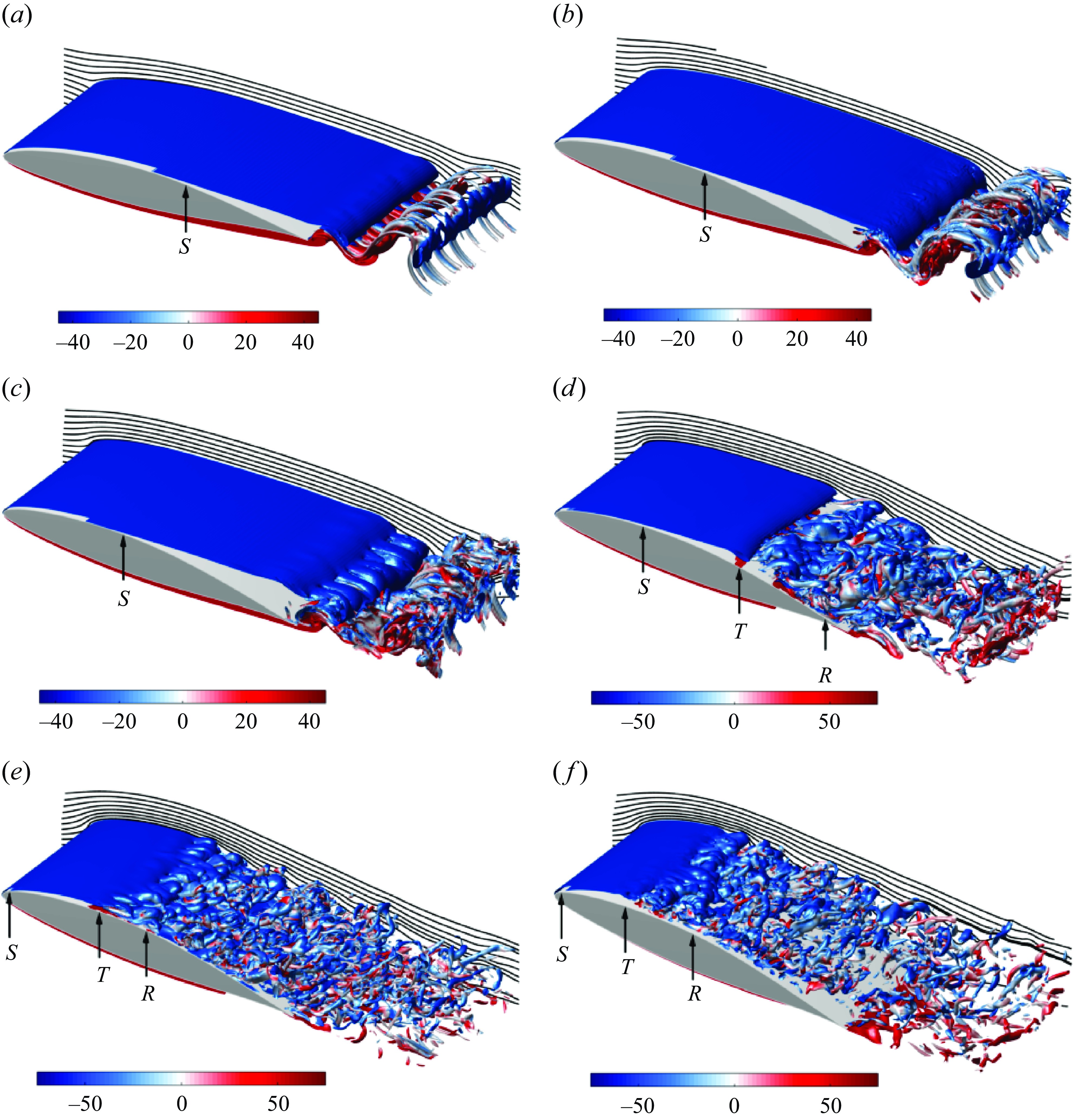
Figure 6. Iso-vorticity surfaces for
 $\alpha$
from 0
$\alpha$
from 0
 $^{\circ }$
(a) to 10
$^{\circ }$
(a) to 10
 $^{\circ }$
(f). Here, S, T and R indicate the mean locations of separation, transition and reattachment.
$^{\circ }$
(f). Here, S, T and R indicate the mean locations of separation, transition and reattachment.
The case of SI – separation without reattachment
Laminar separation without reattachment is observed at
 $\alpha$
from 0
$\alpha$
from 0
 $^{\circ }$
to 6
$^{\circ }$
to 6
 $^{\circ }$
(i.e. open separation). The separation point S is defined as the time-averaged location of zero skin friction, and is located at
$^{\circ }$
(i.e. open separation). The separation point S is defined as the time-averaged location of zero skin friction, and is located at
 $x_{s,0^{\circ }}/c$
= 0.6,
$x_{s,0^{\circ }}/c$
= 0.6,
 $x_{s,4^{\circ }}/$
c = 0.49 and
$x_{s,4^{\circ }}/$
c = 0.49 and
 $x_{s,6^{\circ }}/c$
= 0.4, as shown in figure 6(a)–(c). For
$x_{s,6^{\circ }}/c$
= 0.4, as shown in figure 6(a)–(c). For
 $\alpha$
= 0
$\alpha$
= 0
 $^{\circ }$
and
$^{\circ }$
and
 $4^{\circ }$
, the flow over the airfoil is quasi-two dimensional and 3-D structures develop only at the trailing edge and in the wake. The wake roll-up itself is strongly influenced by the positive, counter-clockwise vortex shed at the trailing edge and originating on the pressure-side boundary layer (coloured red in figure 6(a)–(c). Although the wake flow is initially quite uniform in the spanwise direction, there is a regular variation in
$4^{\circ }$
, the flow over the airfoil is quasi-two dimensional and 3-D structures develop only at the trailing edge and in the wake. The wake roll-up itself is strongly influenced by the positive, counter-clockwise vortex shed at the trailing edge and originating on the pressure-side boundary layer (coloured red in figure 6(a)–(c). Although the wake flow is initially quite uniform in the spanwise direction, there is a regular variation in
 $z$
as streamwise vortices develop on the primary wake mode. The closure of the wake seen in the time averages of figure 5 (a)–(b) comes as the suction surface shear layer wraps over the coherent trailing-edge vortex from the pressure side.
$z$
as streamwise vortices develop on the primary wake mode. The closure of the wake seen in the time averages of figure 5 (a)–(b) comes as the suction surface shear layer wraps over the coherent trailing-edge vortex from the pressure side.
At
 $\alpha$
= 6
$\alpha$
= 6
 $^{\circ }$
, a KH instability leads to the development of spanwise vortices within the separated, upper shear layer with undulations appearing upstream of the trailing edge (figure 6
c). The postulated KH instability can be supported by observations in the vertical velocity (
$^{\circ }$
, a KH instability leads to the development of spanwise vortices within the separated, upper shear layer with undulations appearing upstream of the trailing edge (figure 6
c). The postulated KH instability can be supported by observations in the vertical velocity (
 $v$
) field along the separated shear layer on the suction side as follows: figure 7 shows its space–time diagram on the left and the corresponding power spectral density (PSD) (Welch’s estimate) is given on the right for two locations (identified by the two dashed lines in the space–time diagram). In the figure, the top row shows the suction side and bottom row the pressure-side shear layer. On the suction side, major frequency peaks in the spectra occur at
$v$
) field along the separated shear layer on the suction side as follows: figure 7 shows its space–time diagram on the left and the corresponding power spectral density (PSD) (Welch’s estimate) is given on the right for two locations (identified by the two dashed lines in the space–time diagram). In the figure, the top row shows the suction side and bottom row the pressure-side shear layer. On the suction side, major frequency peaks in the spectra occur at
 $fc/u_\infty$
= 2.2 and
$fc/u_\infty$
= 2.2 and
 $fc/u_\infty$
= 4.5 and the streaks in the space–time diagram have a positive inclination that indicates downstream movement (and amplification) of the perturbation waves. On the pressure side, a single peak occurs at
$fc/u_\infty$
= 4.5 and the streaks in the space–time diagram have a positive inclination that indicates downstream movement (and amplification) of the perturbation waves. On the pressure side, a single peak occurs at
 $fc/u_\infty$
= 2.2 and the streaks in the space–time diagram have a negative slope – a footprint of the upstream-travelling pressure waves generated by the trailing-edge vortex shedding.
$fc/u_\infty$
= 2.2 and the streaks in the space–time diagram have a negative slope – a footprint of the upstream-travelling pressure waves generated by the trailing-edge vortex shedding.
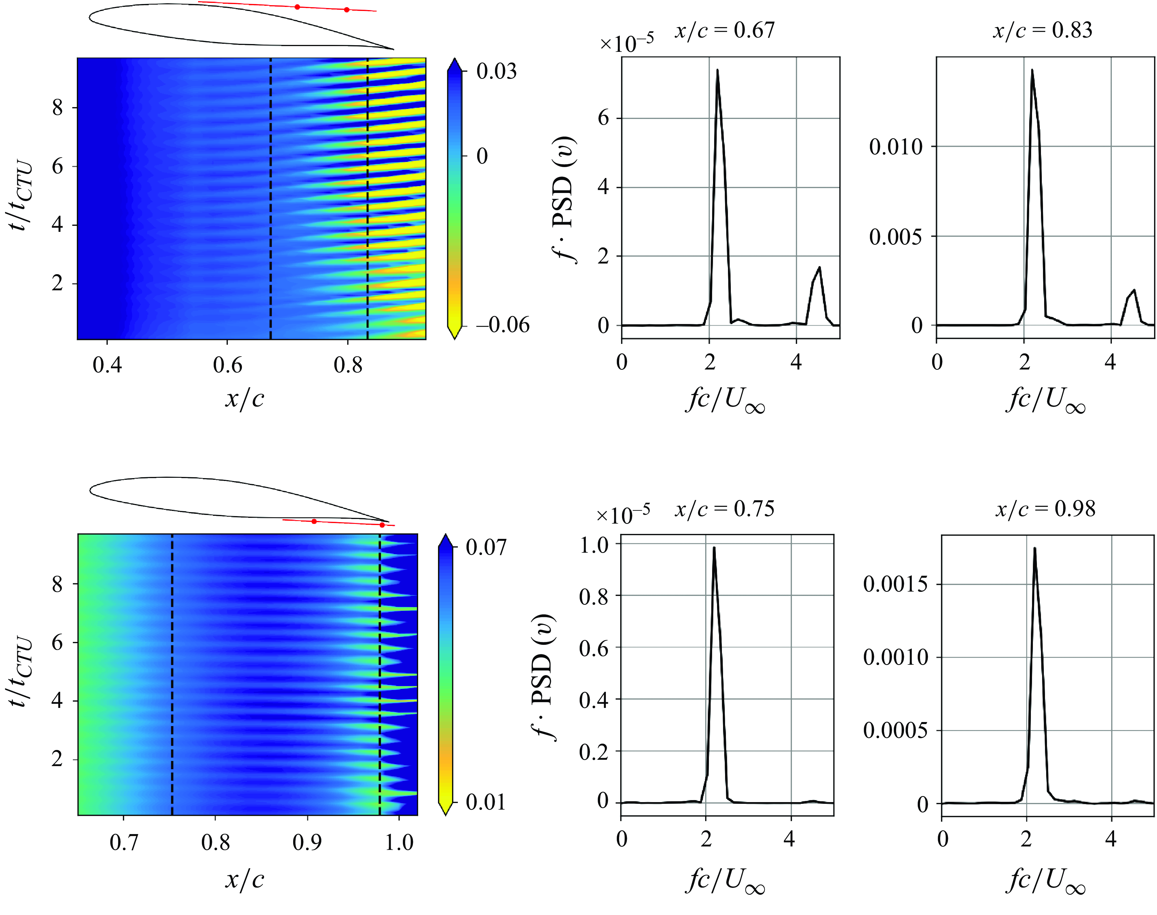
Figure 7. Space–time diagram of the vertical velocity component (
 $v$
) along the shear layer (left) for
$v$
) along the shear layer (left) for
 $\alpha$
= 6
$\alpha$
= 6
 $^{\circ }$
. The PSD at two locations (indicated by dashed lines) on the right. Top: suction side, bottom: pressure side.
$^{\circ }$
. The PSD at two locations (indicated by dashed lines) on the right. Top: suction side, bottom: pressure side.
By calculating the Strouhal number based on the momentum thickness of the shear layer at the separation point
 $\theta _{\textit{SP}}$
= 0.0035
$\theta _{\textit{SP}}$
= 0.0035
 $c$
and the maximum velocity magnitude on the upper side of the separated shear layer
$c$
and the maximum velocity magnitude on the upper side of the separated shear layer
 $\|\mathbf {u}\|_e$
, a Strouhal number of
$\|\mathbf {u}\|_e$
, a Strouhal number of
 $\mathrm {St}_{\textit{KH}}=f_{\textit{KH}}\theta_{\textit{SP}}/$
 $\|\mathbf {u}\|_e$
= 0.006 is found for the mode at
$\|\mathbf {u}\|_e$
= 0.006 is found for the mode at
 $fc/u_\infty$
= 2.2 and
$fc/u_\infty$
= 2.2 and
 $\mathrm {St}_{\textit{KH}}$
= 0.013 is found for the mode at the second peak
$\mathrm {St}_{\textit{KH}}$
= 0.013 is found for the mode at the second peak
 $fc/u_\infty$
= 4.5. These values agree well with compiled data by McAuliffe & Yara (Reference McAuliffe and Yara2009) for KH instabilities showing a range of 0.005
$fc/u_\infty$
= 4.5. These values agree well with compiled data by McAuliffe & Yara (Reference McAuliffe and Yara2009) for KH instabilities showing a range of 0.005
 $\leqslant$
 $\mathrm {St}_{\textit{KH}}$
 $\leqslant$
0.016. Hence, we conclude this higher-frequency mode is a KH instability occurring only within the separated shear layer while the lower-frequency peaks at
$\leqslant$
0.016. Hence, we conclude this higher-frequency mode is a KH instability occurring only within the separated shear layer while the lower-frequency peaks at
 $fc/u_\infty$
= 2.2, which occur on both suction and pressure sides, are footprints of the vortex shedding at the trailing edge.
$fc/u_\infty$
= 2.2, which occur on both suction and pressure sides, are footprints of the vortex shedding at the trailing edge.
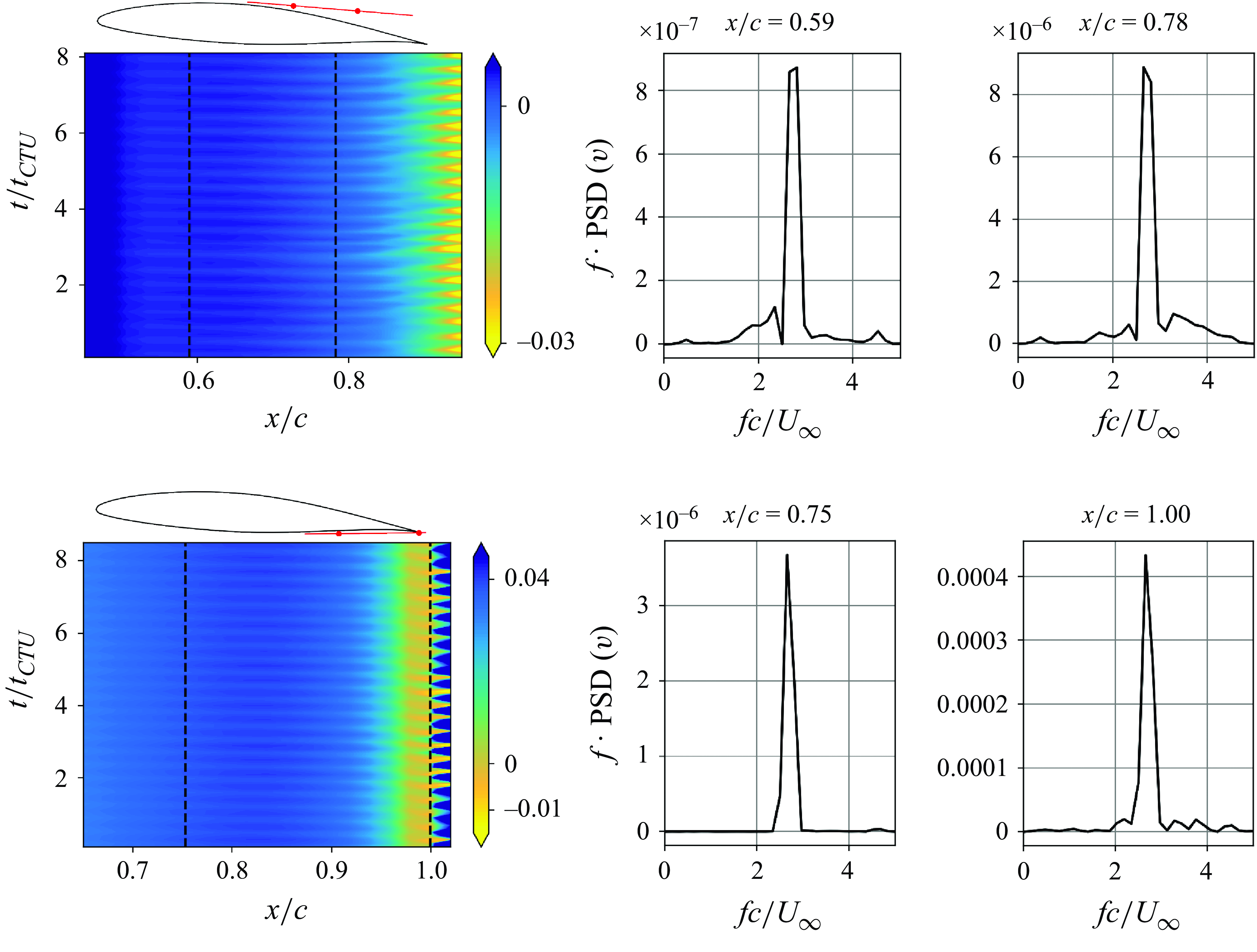
Figure 8. Space–time diagram of the lateral velocity component (
 $v$
) along the shear layer (left) for
$v$
) along the shear layer (left) for
 $\alpha$
= 4
$\alpha$
= 4
 $^{\circ }$
. The PSD at two locations (indicated by dashed lines) on the right. Top: suction side, bottom: pressure side.
$^{\circ }$
. The PSD at two locations (indicated by dashed lines) on the right. Top: suction side, bottom: pressure side.
At lower incidence (
 $\alpha$
= 4
$\alpha$
= 4
 $^{\circ }$
), the space–time diagram shows distinct peaks at Strouhal numbers
$^{\circ }$
), the space–time diagram shows distinct peaks at Strouhal numbers
 $fc/u_\infty$
= 2.8 on both the suction side and the pressure side (figure 8). The inclination of the streaks along the suction-side shear layer is, however, negative for
$fc/u_\infty$
= 2.8 on both the suction side and the pressure side (figure 8). The inclination of the streaks along the suction-side shear layer is, however, negative for
 $x/c$
< 0.8, indicating that this mode does not travel downstream, as it did for the
$x/c$
< 0.8, indicating that this mode does not travel downstream, as it did for the
 $\alpha$
= 6
$\alpha$
= 6
 $^{\circ }$
case, but travels upstream on both sides of the airfoil. This suggests that the shear layer in this case is not subject to a growing KH instability, but is affected by perturbation waves from the trailing-edge shedding of the pressure-side shear layer.
$^{\circ }$
case, but travels upstream on both sides of the airfoil. This suggests that the shear layer in this case is not subject to a growing KH instability, but is affected by perturbation waves from the trailing-edge shedding of the pressure-side shear layer.
Now there is a regular modulation of the suction-side shear layer, with a spanwise wavelength similar to the streamwise braids that develop in the near wake. The growth of the instability is, however, not fast enough to cause the flow to reattach and the separated shear layer encloses a large recirculation region between the separation point and the trailing edge for
 $\alpha$
from
$\alpha$
from
 $0^{\circ }$
to
$0^{\circ }$
to
 $6^{\circ }$
.
$6^{\circ }$
.
The special case at
 $\alpha _{\textit{crit}}$
– the flow reattaches
$\alpha _{\textit{crit}}$
– the flow reattaches

At
 $\alpha$
= 7
$\alpha$
= 7
 $^{\circ }$
, the flow separates at
$^{\circ }$
, the flow separates at
 $x_{s,7^{\circ }}/c$
= 0.26 and a KH instability drives the formation of large, spanwise vortices along the separated shear layer in the region 0.5
$x_{s,7^{\circ }}/c$
= 0.26 and a KH instability drives the formation of large, spanwise vortices along the separated shear layer in the region 0.5
 $\leqslant$
 $x/c$
$x/c$
 $\leqslant$
0.6. Upon their generation, these vortices are quasi-two-dimensional but lose their coherence as they roll over the airfoil surface and transition into turbulence at
$\leqslant$
0.6. Upon their generation, these vortices are quasi-two-dimensional but lose their coherence as they roll over the airfoil surface and transition into turbulence at
 $x_{t,7^{\circ }}/c$
= 0.62 (marked as T in figure 6). The structure of the turbulent reattachment is of course complicated, but traces of the spanwise structures observed at lower
$x_{t,7^{\circ }}/c$
= 0.62 (marked as T in figure 6). The structure of the turbulent reattachment is of course complicated, but traces of the spanwise structures observed at lower
 $\alpha$
can be still be seen at this angle of attack.
$\alpha$
can be still be seen at this angle of attack.
As is well known, the turbulent fluid motion transports momentum from the mean flow towards the airfoil surface and re-energises the boundary layer, resulting in the reattachment of the flow at
 $x_{r,7^{\circ }}/c$
= 0.93 (see figure 6
d). The turbulent reattachment at the trailing-edge results in a slender LSB that has a maximum wall-normal height of
$x_{r,7^{\circ }}/c$
= 0.93 (see figure 6
d). The turbulent reattachment at the trailing-edge results in a slender LSB that has a maximum wall-normal height of
 $h_{\textit{LSB}}$
= 3.3 % of the chord length and stretches over 67 % of the airfoil.
$h_{\textit{LSB}}$
= 3.3 % of the chord length and stretches over 67 % of the airfoil.
The case of SII – thin bubble with reattachment
With an increase of the angle of attack beyond
 $\alpha$
= 7
$\alpha$
= 7
 $^{\circ }$
the LSB abruptly shifts from the trailing edge of the airfoil to the leading edge with the flow separating at
$^{\circ }$
the LSB abruptly shifts from the trailing edge of the airfoil to the leading edge with the flow separating at
 $x_{s,8^{\circ }}/c$
= 0.014 and reattaching at mid-chord (
$x_{s,8^{\circ }}/c$
= 0.014 and reattaching at mid-chord (
 $x_{r,8^{\circ }}/c$
= 0.48) (see figure 6
e for
$x_{r,8^{\circ }}/c$
= 0.48) (see figure 6
e for
 $\alpha$
= 8
$\alpha$
= 8
 $^{\circ }$
). The proportions of the LSB are similar to those at
$^{\circ }$
). The proportions of the LSB are similar to those at
 $\alpha$
= 7
$\alpha$
= 7
 $^{\circ }$
, with the bubble height measuring
$^{\circ }$
, with the bubble height measuring
 $h_{\textit{LSB}}$
= 2.5 % of the chord length and the ratios of LSB height to length being 0.054 (8
$h_{\textit{LSB}}$
= 2.5 % of the chord length and the ratios of LSB height to length being 0.054 (8
 $^{\circ }$
) and 0.052 (7
$^{\circ }$
) and 0.052 (7
 $^{\circ }$
). At
$^{\circ }$
). At
 $\alpha$
= 8
$\alpha$
= 8
 $^{\circ }$
, the flow is laminar for the first two thirds of the bubble length at which point (
$^{\circ }$
, the flow is laminar for the first two thirds of the bubble length at which point (
 $x_{t,8^{\circ }}/c$
= 0.32) the separated shear layer transitions. The topology downstream of the transition point is characterised by hairpin vortices and the break up of the laminar, spanwise vortices that shed off the LSB shear layer. Horseshoe, hairpin or loop vortices all describe vortex tubes that, starting from a cross-stream alignment, bend upwards away from the wall and stretch in the streamwise direction as the upper portion (head) is subjected to the higher velocity in the boundary layer (Robinson Reference Robinson1991). As the bubble trailing edge shifts from
$x_{t,8^{\circ }}/c$
= 0.32) the separated shear layer transitions. The topology downstream of the transition point is characterised by hairpin vortices and the break up of the laminar, spanwise vortices that shed off the LSB shear layer. Horseshoe, hairpin or loop vortices all describe vortex tubes that, starting from a cross-stream alignment, bend upwards away from the wall and stretch in the streamwise direction as the upper portion (head) is subjected to the higher velocity in the boundary layer (Robinson Reference Robinson1991). As the bubble trailing edge shifts from
 $x_{r,7^{\circ }}/c$
= 0.93 at
$x_{r,7^{\circ }}/c$
= 0.93 at
 $\alpha$
= 7
$\alpha$
= 7
 $^{\circ }$
to
$^{\circ }$
to
 $x_{r,8^{\circ }}/c$
= 0.48 at
$x_{r,8^{\circ }}/c$
= 0.48 at
 $\alpha$
= 8
$\alpha$
= 8
 $^{\circ }$
, the turbulent boundary layer occupies the remainder of the suction surface, advecting into the wake as fine-scale structures with little obvious regular pattern. A similar flow state is found at
$^{\circ }$
, the turbulent boundary layer occupies the remainder of the suction surface, advecting into the wake as fine-scale structures with little obvious regular pattern. A similar flow state is found at
 $\alpha$
= 10
$\alpha$
= 10
 $^{\circ }$
, where the LSB has slightly changed in size with an earlier transition point (
$^{\circ }$
, where the LSB has slightly changed in size with an earlier transition point (
 $x_{t,10^{\circ }}/c$
= 0.23), marginally shorter bubble length (
$x_{t,10^{\circ }}/c$
= 0.23), marginally shorter bubble length (
 $x_{s,10^{\circ }}/c$
= 0.012,
$x_{s,10^{\circ }}/c$
= 0.012,
 $x_{r,10^{\circ }}/c$
= 0.46) and increased height
$x_{r,10^{\circ }}/c$
= 0.46) and increased height
 $h_{\textit{LSB}}/c$
= 3.9 %. The height-to-length ratio consequently increases to 0.087, which is more than 60 % greater than the values found at
$h_{\textit{LSB}}/c$
= 3.9 %. The height-to-length ratio consequently increases to 0.087, which is more than 60 % greater than the values found at
 $\alpha$
= 7
$\alpha$
= 7
 $^{\circ }$
and 8
$^{\circ }$
and 8
 $^{\circ }$
.
$^{\circ }$
.
4.3. Flow structure and instability
In the specific context of LSBs and their dynamics, the studies by Jones et al. (Reference Jones, Sandberg and Sandham2008) and later by Marxen et al. (Reference Marxen, Lang and Rist2013) describe self-sustained turbulence in an LSB being driven by a combination of elliptic instability within the KH vortices and hyperbolic shear instabilities between them. While the flow over the NACA 65(1)–412 certainly shares some similarities, its transition from an open separation at low
 $\alpha$
to reattachment and establishment of an LSB first at the trailing edge and then at the leading edge at high
$\alpha$
to reattachment and establishment of an LSB first at the trailing edge and then at the leading edge at high
 $\alpha$
yields a much larger variety of different vortex dynamics and 3-D instability mechanisms, which we will discuss in the following paragraphs.
$\alpha$
yields a much larger variety of different vortex dynamics and 3-D instability mechanisms, which we will discuss in the following paragraphs.
4.3.1. The case of SI and low
$\alpha$

Figure 9 visualises vortical structures at the trailing edge for
 $\alpha$
= 0
$\alpha$
= 0
 $^{\circ }, 4^{\circ }, \;\textrm {and} \; 6^{\circ }$
through iso-surface plots of
$^{\circ }, 4^{\circ }, \;\textrm {and} \; 6^{\circ }$
through iso-surface plots of
 $Q$
$Q$
 $\equiv$
 $(u_{i,i}^2 - u_{i,j}u_{j,i})/2$
(Jeong & Hussain Reference Jeong and Hussain1995), coloured according to the spanwise vorticity component
$(u_{i,i}^2 - u_{i,j}u_{j,i})/2$
(Jeong & Hussain Reference Jeong and Hussain1995), coloured according to the spanwise vorticity component
 $\omega _z$
.
$\omega _z$
.
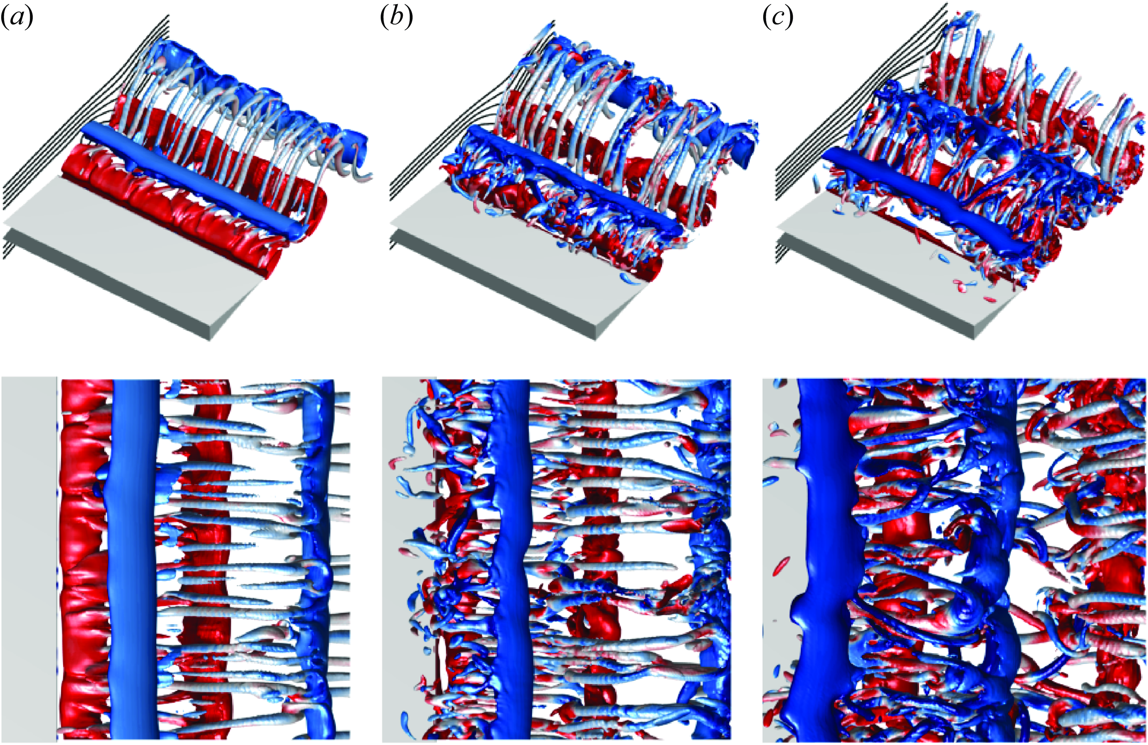
Figure 9. Trailing-edge view of iso-
 $Q$
surfaces for
$Q$
surfaces for
 $\alpha$
= 0
$\alpha$
= 0
 $^{\circ }$
(a), 4
$^{\circ }$
(a), 4
 $^{\circ }$
(b) and 6
$^{\circ }$
(b) and 6
 $^{\circ }$
(c). Colouring is by spanwise vorticity
$^{\circ }$
(c). Colouring is by spanwise vorticity
 $\omega _z$
.
$\omega _z$
.
Figure 9 shows the emergence of a series of streamwise loop vortices that originate from the vortex roll-up at the trailing edge and, as the flow angle increases from 0
 $^{\circ }$
to 4
$^{\circ }$
to 4
 $^{\circ }$
and 6
$^{\circ }$
and 6
 $^{\circ }$
, combine into clusters of longitudinal coherent vortex structures with a tubular shape. The wake structure and its development is especially clear for the
$^{\circ }$
, combine into clusters of longitudinal coherent vortex structures with a tubular shape. The wake structure and its development is especially clear for the
 $\alpha = 0^{\circ }$
case in figure 9(a). A first vortex forms from the positive spanwise rolled up sheet originating from the pressure-side trailing edge. On this sheet and vortex, approximately four spanwise modulations can already be identified. The same spanwise wavelength modulations can be seen in the opposite-signed roll-up from the suction-side shear layer. Immediately behind the clockwise roller, the original modulations in the counter-clockwise counterpart become clear and are associated with thin, streamwise vortices that connect successive spanwise structures. The same basic structure is observed as
$\alpha = 0^{\circ }$
case in figure 9(a). A first vortex forms from the positive spanwise rolled up sheet originating from the pressure-side trailing edge. On this sheet and vortex, approximately four spanwise modulations can already be identified. The same spanwise wavelength modulations can be seen in the opposite-signed roll-up from the suction-side shear layer. Immediately behind the clockwise roller, the original modulations in the counter-clockwise counterpart become clear and are associated with thin, streamwise vortices that connect successive spanwise structures. The same basic structure is observed as
 $\alpha$
increases to
$\alpha$
increases to
 $4^{\circ }$
(figure 9
b) although the filaments or braids have moved upstream onto the airfoil surface. At
$4^{\circ }$
(figure 9
b) although the filaments or braids have moved upstream onto the airfoil surface. At
 $\alpha = 6^{\circ }$
(figure 9
c) the first vortex is now the clockwise vortex from the suction-side shear layer and the near wake has become more chaotic with longer-wavelength modes that appear to be mixed in with the streamwise braids. In the following, we quantify the scales of the flow structures, i.e. the vortex cores and the braid, within the near wake.
$\alpha = 6^{\circ }$
(figure 9
c) the first vortex is now the clockwise vortex from the suction-side shear layer and the near wake has become more chaotic with longer-wavelength modes that appear to be mixed in with the streamwise braids. In the following, we quantify the scales of the flow structures, i.e. the vortex cores and the braid, within the near wake.
As pointed out by Deng et al. (Reference Deng, Sun and Shao2017), basing the characteristic length on the projected frontal height of the airfoil (
 $c\cdot \sin {\alpha }$
) rather then on the chord length
$c\cdot \sin {\alpha }$
) rather then on the chord length
 $c$
results in very similar values for the critical Reynolds numbers to those found in bluff body wakes. Williamson (Reference Williamson1996b
) and later Jones et al. (Reference Jones, Sandberg and Sandham2008) based their scaling on the diameter of the vortices themselves. If we assume that the vortices shed at the airfoil’s trailing edge also scale with the projected frontal area, both approaches should deliver similar values for the characteristic spanwise wavelengths of the vortex instabilities. We therefore also use the vortex diameter in the following as a characteristic length scale, but for completeness we note that the projected frontal height of the NACA 65(1)–412 ranges from 0.12
$c$
results in very similar values for the critical Reynolds numbers to those found in bluff body wakes. Williamson (Reference Williamson1996b
) and later Jones et al. (Reference Jones, Sandberg and Sandham2008) based their scaling on the diameter of the vortices themselves. If we assume that the vortices shed at the airfoil’s trailing edge also scale with the projected frontal area, both approaches should deliver similar values for the characteristic spanwise wavelengths of the vortex instabilities. We therefore also use the vortex diameter in the following as a characteristic length scale, but for completeness we note that the projected frontal height of the NACA 65(1)–412 ranges from 0.12
 $c$
(
$c$
(
 $\alpha$
= 0
$\alpha$
= 0
 $^{\circ }$
) to 0.15
$^{\circ }$
) to 0.15
 $c$
(
$c$
(
 $\alpha$
= 6
$\alpha$
= 6
 $^{\circ }$
). The average diameter of the near-wake Kármán vortices, as measured by the minor axis diameter
$^{\circ }$
). The average diameter of the near-wake Kármán vortices, as measured by the minor axis diameter
 $d_{max}$
of the elliptical streamline passing through the maximum circumferential velocity of the vortex (following the lines of Williamson Reference Williamson1996b
), is approximately
$d_{max}$
of the elliptical streamline passing through the maximum circumferential velocity of the vortex (following the lines of Williamson Reference Williamson1996b
), is approximately
 $d_{\textit{core}}$
= 0.04
$d_{\textit{core}}$
= 0.04
 $c$
–0.06
$c$
–0.06
 $c$
. We note that the same diameters are also obtained by measuring the region of positive
$c$
. We note that the same diameters are also obtained by measuring the region of positive
 $Q$
. A more detailed study on the vortex diameter is provided later in § 4.3.3. The vortex diameter measures are given in figure 10, where the velocity at each measured vortex core is subtracted from the field to produce the plotted streamline pattern. The values closely match the vortex diameter of 0.05
$Q$
. A more detailed study on the vortex diameter is provided later in § 4.3.3. The vortex diameter measures are given in figure 10, where the velocity at each measured vortex core is subtracted from the field to produce the plotted streamline pattern. The values closely match the vortex diameter of 0.05
 $c$
reported for the LSB shedding over the NACA 0012 at a Reynolds number of
$c$
reported for the LSB shedding over the NACA 0012 at a Reynolds number of
 $5\times 10^4$
(Jones et al. Reference Jones, Sandberg and Sandham2008).
$5\times 10^4$
(Jones et al. Reference Jones, Sandberg and Sandham2008).
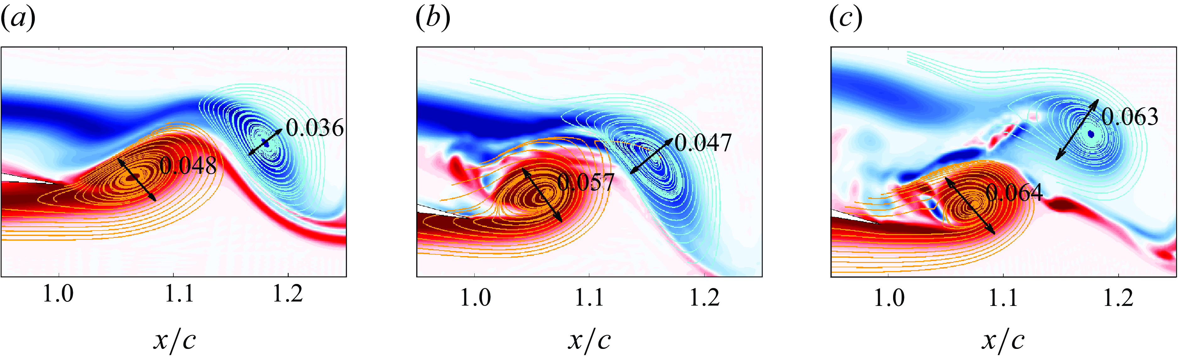
Figure 10. Streamlines of the pressure-side (orange) and suction-side (blue) vortices for
 $\alpha$
= 0
$\alpha$
= 0
 $^{\circ }$
(a), 4
$^{\circ }$
(a), 4
 $^{\circ }$
(b) and 6
$^{\circ }$
(b) and 6
 $^{\circ }$
(c). Streamlines are generated by subtracting the velocity at the respective vortex centres. Colouring is by spanwise vorticity
$^{\circ }$
(c). Streamlines are generated by subtracting the velocity at the respective vortex centres. Colouring is by spanwise vorticity
 $\omega _z$
.
$\omega _z$
.

Figure 11. The PSD of the spanwise vorticity
 $\omega _z$
along the span for the vortex cores and the braid region located downstream of evaluated core. Bottom row: snapshots of spanwise-averaged
$\omega _z$
along the span for the vortex cores and the braid region located downstream of evaluated core. Bottom row: snapshots of spanwise-averaged
 $\omega _z$
contours with vortex cores (white
$\omega _z$
contours with vortex cores (white
 $\times$
) and braid location (black
$\times$
) and braid location (black
 $\ast$
).
$\ast$
).
For the wake transition behind a circular cylinder of diameter
 $D$
, the elliptic mode A instability is expected to lead to modes with wavelengths of 3
$D$
, the elliptic mode A instability is expected to lead to modes with wavelengths of 3
 $D$
–4
$D$
–4
 $D$
, where the vortex cores were estimated to scale as
$D$
, where the vortex cores were estimated to scale as
 $d_{\textit{core}}$
 $\approx$
 $D$
(Leweke & Williamson Reference Williamson1998b
). Other values of
$D$
(Leweke & Williamson Reference Williamson1998b
). Other values of
 $\lambda _z$
= 2
$\lambda _z$
= 2
 $d_{\textit{inv}}$
(with the diameter of the invariant streamtube
$d_{\textit{inv}}$
(with the diameter of the invariant streamtube
 $d_{\textit{inv}}$
) have, however, been found by theoretical predictions and were confirmed by experiment (Leweke & Williamson Reference Leweke and Williamson1998a
) and simulation (Laporte & Corjon Reference Laporte and Corjon2000). We therefore expect the elliptic instability to induce perturbations with a spanwise wavelength in the range 0.08
$d_{\textit{inv}}$
) have, however, been found by theoretical predictions and were confirmed by experiment (Leweke & Williamson Reference Leweke and Williamson1998a
) and simulation (Laporte & Corjon Reference Laporte and Corjon2000). We therefore expect the elliptic instability to induce perturbations with a spanwise wavelength in the range 0.08
 $c$
$c$
 $\leqslant$
 $\lambda _{z}$
 $\leqslant$
0.18
$\leqslant$
0.18
 $c$
, or 3–6 waves per span. Accordingly, the hyperbolic mode B instability would be expected to lead to 12–24 waves per span (assuming quadrupling). The occurrence of a true mode B instability is, however, unlikely if we follow the Floquet analysis of low-Reynolds-number airfoil wakes (Meneghini et al. Reference Meneghini, Carmo, Tsiloufas, Gioria and Aranha2011; Deng et al. Reference Deng, Sun and Shao2017; Gupta et al. Reference Gupta, Zhao, Sharma, Agrawal, Hourigan and Thompson2022) and the high-wavenumber instability is more likely to be of mode C type (which shares similarities with modes A and B) and was found to grow fastest for NACA airfoils at low Reynolds number. The Floquet analysis by Gupta et al. (Reference Gupta, Zhao, Sharma, Agrawal, Hourigan and Thompson2022) revealed a ratio of spanwise wavelengths between mode A and mode C of approximately
$c$
, or 3–6 waves per span. Accordingly, the hyperbolic mode B instability would be expected to lead to 12–24 waves per span (assuming quadrupling). The occurrence of a true mode B instability is, however, unlikely if we follow the Floquet analysis of low-Reynolds-number airfoil wakes (Meneghini et al. Reference Meneghini, Carmo, Tsiloufas, Gioria and Aranha2011; Deng et al. Reference Deng, Sun and Shao2017; Gupta et al. Reference Gupta, Zhao, Sharma, Agrawal, Hourigan and Thompson2022) and the high-wavenumber instability is more likely to be of mode C type (which shares similarities with modes A and B) and was found to grow fastest for NACA airfoils at low Reynolds number. The Floquet analysis by Gupta et al. (Reference Gupta, Zhao, Sharma, Agrawal, Hourigan and Thompson2022) revealed a ratio of spanwise wavelengths between mode A and mode C of approximately
 $\lambda _{\textit{Mode A}}/\lambda _{\textit{Mode C}}$
 $\approx$
3, which is 9–18 waves per span for the current flow.
$\approx$
3, which is 9–18 waves per span for the current flow.
We quantify the spanwise wavenumbers by extracting a PSD estimate of the streamwise vorticity
 $\omega _x$
along the span in the near-wake (
$\omega _x$
along the span in the near-wake (
 $x\,\gt \,1.05$
) vortex cores and braid regions in figure 11. The primary vortex cores from the Strouhal shedding with
$x\,\gt \,1.05$
) vortex cores and braid regions in figure 11. The primary vortex cores from the Strouhal shedding with
 $\omega _z\,\lt \,0$
(suction-side (SS) shear layer roll-up) are identified by the blue filled circles and the cores with
$\omega _z\,\lt \,0$
(suction-side (SS) shear layer roll-up) are identified by the blue filled circles and the cores with
 $\omega _z\,\gt \,0$
(pressure-side (PS) shear layer roll-up) by orange filled circles. It is consistently observed for angles (
$\omega _z\,\gt \,0$
(pressure-side (PS) shear layer roll-up) by orange filled circles. It is consistently observed for angles (
 $0^{\circ }\,\leqslant \,\alpha \,\leqslant \,6^{\circ }$
) that the amplitude of the spanwise mode within the SS cores is approximately half the values found along the PS cores. The figures show that the vortex cores are subject to lower wavenumber perturbations than the braid region, as indicated by a shift in the peaks in figure 11. Specifically, the spectrum indicates that 6–8 (first and second peak) braid loop pairs are present over the span (
$0^{\circ }\,\leqslant \,\alpha \,\leqslant \,6^{\circ }$
) that the amplitude of the spanwise mode within the SS cores is approximately half the values found along the PS cores. The figures show that the vortex cores are subject to lower wavenumber perturbations than the braid region, as indicated by a shift in the peaks in figure 11. Specifically, the spectrum indicates that 6–8 (first and second peak) braid loop pairs are present over the span (
 $0.5c$
) at
$0.5c$
) at
 $\alpha = 0^{\circ }$
, while the PS vortex has 4–6 perturbation waves and the SS vortex has a peak at only 2 waves per span (note that the discrete values of
$\alpha = 0^{\circ }$
, while the PS vortex has 4–6 perturbation waves and the SS vortex has a peak at only 2 waves per span (note that the discrete values of
 $k_z c /2\pi$
in the figure give the number of waves over one chord length, or twice the span). The perturbation wavenumbers at
$k_z c /2\pi$
in the figure give the number of waves over one chord length, or twice the span). The perturbation wavenumbers at
 $\alpha = 4^{\circ }$
show peaks for the Strouhal vortices of 4 (SS) and 5 (PS) waves per span and 6–9 braid loop pairs. At
$\alpha = 4^{\circ }$
show peaks for the Strouhal vortices of 4 (SS) and 5 (PS) waves per span and 6–9 braid loop pairs. At
 $\alpha = 6^{\circ }$
, the spectrum is broader compared with the lower angles caused by the wake transition, which is already strongly disturbing the 2-D flow at the trailing edge. Nevertheless, peaks in the spectrum indicate dominant modes at 2 and 4 waves per span within the Strouhal vortex cores and 4 waves within the braid region. The range of 2–6 waves per span (0.5
$\alpha = 6^{\circ }$
, the spectrum is broader compared with the lower angles caused by the wake transition, which is already strongly disturbing the 2-D flow at the trailing edge. Nevertheless, peaks in the spectrum indicate dominant modes at 2 and 4 waves per span within the Strouhal vortex cores and 4 waves within the braid region. The range of 2–6 waves per span (0.5
 $c$
) for the dominant modes in the spectra (figure 11) match very well with the expected spanwise wavelength of mode A (3–6 waves). The secondary peaks that exist at the higher wavenumbers with 8–9 waves per span point to an additional instability matching the predicted wavelengths of mode C.
$c$
) for the dominant modes in the spectra (figure 11) match very well with the expected spanwise wavelength of mode A (3–6 waves). The secondary peaks that exist at the higher wavenumbers with 8–9 waves per span point to an additional instability matching the predicted wavelengths of mode C.
While the original streamwise vortices are rather evenly distributed at 0
 $^{\circ }$
, they begin to cluster at 4
$^{\circ }$
, they begin to cluster at 4
 $^{\circ }$
and most notably at 6
$^{\circ }$
and most notably at 6
 $^{\circ }$
, while the primary Kármán vortices increasingly deform compared with the topology at 0
$^{\circ }$
, while the primary Kármán vortices increasingly deform compared with the topology at 0
 $^{\circ }$
(see figure 9). This clustering of braids and deformation of the spanwise vortex tubes implies a nonlinear interaction between the secondary braid loops and other modes at different wavelengths (e.g. mode C and mode A within the vortex cores). This observation is supported by the plots in figure 11, where the streamwise vorticity component within the cores shows a tendency towards lower wavenumbers than in the braid region.
$^{\circ }$
(see figure 9). This clustering of braids and deformation of the spanwise vortex tubes implies a nonlinear interaction between the secondary braid loops and other modes at different wavelengths (e.g. mode C and mode A within the vortex cores). This observation is supported by the plots in figure 11, where the streamwise vorticity component within the cores shows a tendency towards lower wavenumbers than in the braid region.
4.3.2. Perturbation analysis at low
$\alpha$

To elaborate on the observations made in the previous paragraphs regarding the dominant modes in the near wake, we track the development of spanwise perturbations with different wavelengths (4
 $\leqslant$
 $k_z c/2\pi$
 $\leqslant$
14) made to an initially 2-D flow field through a set of low-cost simulations with a reduced spanwise resolutions of
$\leqslant$
14) made to an initially 2-D flow field through a set of low-cost simulations with a reduced spanwise resolutions of
 $n_z$
= 39 (
$n_z$
= 39 (
 $\alpha$
= 4
$\alpha$
= 4
 $^{\circ }$
) and
$^{\circ }$
) and
 $n_z$
= 40 (
$n_z$
= 40 (
 $\alpha$
= 6
$\alpha$
= 6
 $^{\circ }$
), similar to Jones et al. (Reference Jones, Sandberg and Sandham2008). The perturbation (
$^{\circ }$
), similar to Jones et al. (Reference Jones, Sandberg and Sandham2008). The perturbation (
 $w_{\mathrm {pert}}$
= 10
$w_{\mathrm {pert}}$
= 10
 $^{-5}$
) is introduced at the airfoil’s trailing edge through a smooth Gaussian distribution function so as to only locally perturb the near wake. The simulations are run for one convective time unit and the growth of the perturbation velocity component
$^{-5}$
) is introduced at the airfoil’s trailing edge through a smooth Gaussian distribution function so as to only locally perturb the near wake. The simulations are run for one convective time unit and the growth of the perturbation velocity component
 $w$
is tracked over time by recording its maximum within the near wake (1
$w$
is tracked over time by recording its maximum within the near wake (1
 $\leqslant$
 $x/c$
$x/c$
 $\leqslant$
1.4), fitting to an exponential function
$\leqslant$
1.4), fitting to an exponential function
 $C_0e^{\sigma t}$
and estimating the associated growth rate
$C_0e^{\sigma t}$
and estimating the associated growth rate
 $\sigma ( w_{max})$
(shown on the left in figures 12 and 13). Details on the extraction of the growth rate are given in Appendix B.
$\sigma ( w_{max})$
(shown on the left in figures 12 and 13). Details on the extraction of the growth rate are given in Appendix B.
The fastest growth occurs at the higher perturbation wavenumbers with a peak at
 $k_z c/2\pi$
= 12 for both
$k_z c/2\pi$
= 12 for both
 $\alpha$
= 4
$\alpha$
= 4
 $^{\circ }$
and 6
$^{\circ }$
and 6
 $^{\circ }$
. This is consistent with the results shown in the previous section, where these modes are also found to dominate the developed flow field. The contour plots of
$^{\circ }$
. This is consistent with the results shown in the previous section, where these modes are also found to dominate the developed flow field. The contour plots of
 $w$
, particularly in figure 12, further show that the perturbation at the higher wavenumber (
$w$
, particularly in figure 12, further show that the perturbation at the higher wavenumber (
 $k_z c/2\pi$
= 12) acts strongly at the edges of the vortices and induces a point-symmetric perturbation within the core (which drives the spanwise bending of the vortex core), while the perturbation is rather uniformly distributed at
$k_z c/2\pi$
= 12) acts strongly at the edges of the vortices and induces a point-symmetric perturbation within the core (which drives the spanwise bending of the vortex core), while the perturbation is rather uniformly distributed at
 $k_z c/2\pi$
= 4 and shows a symmetric pattern.
$k_z c/2\pi$
= 4 and shows a symmetric pattern.
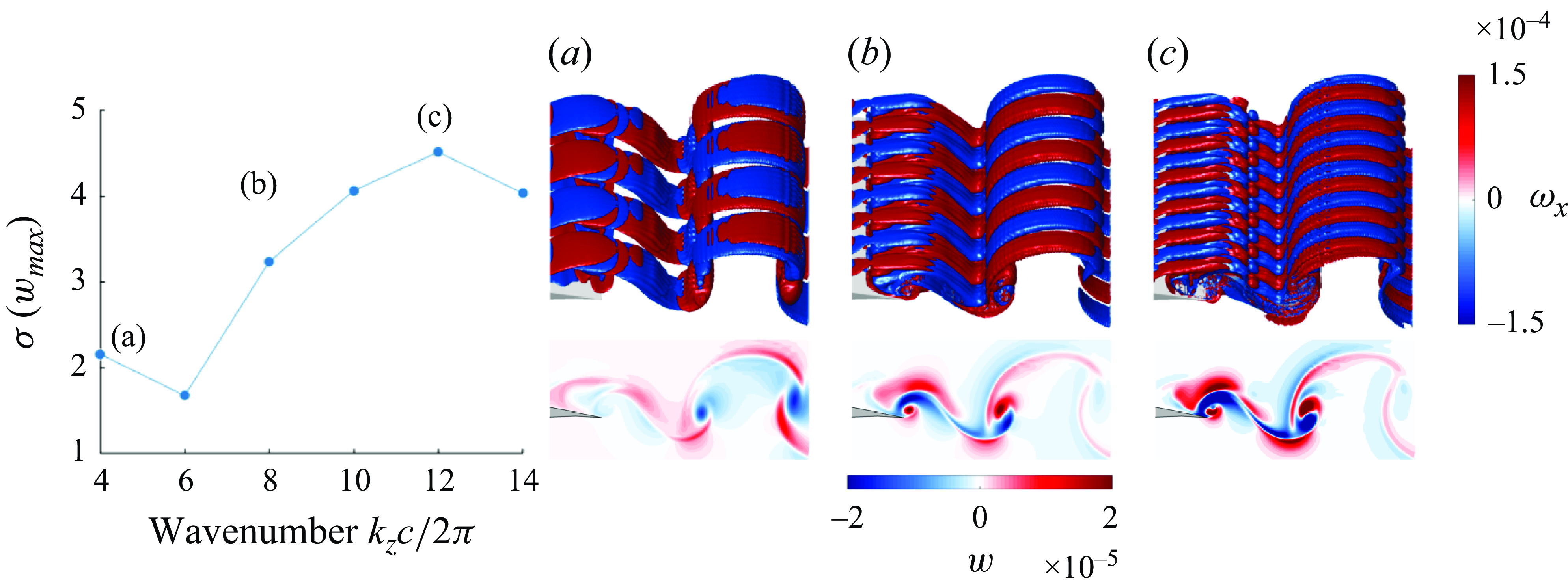
Figure 12. Left: temporal growth rate of
 $w_{max}$
for
$w_{max}$
for
 $\alpha$
= 4
$\alpha$
= 4
 $^{\circ }$
. Top right: iso-
$^{\circ }$
. Top right: iso-
 $\omega _x$
surfaces for wavenumbers 4 (a), 8 (b) and 12 (c) at
$\omega _x$
surfaces for wavenumbers 4 (a), 8 (b) and 12 (c) at
 $t$
= 1.0. Bottom right: corresponding contours of
$t$
= 1.0. Bottom right: corresponding contours of
 $w$
.
$w$
.
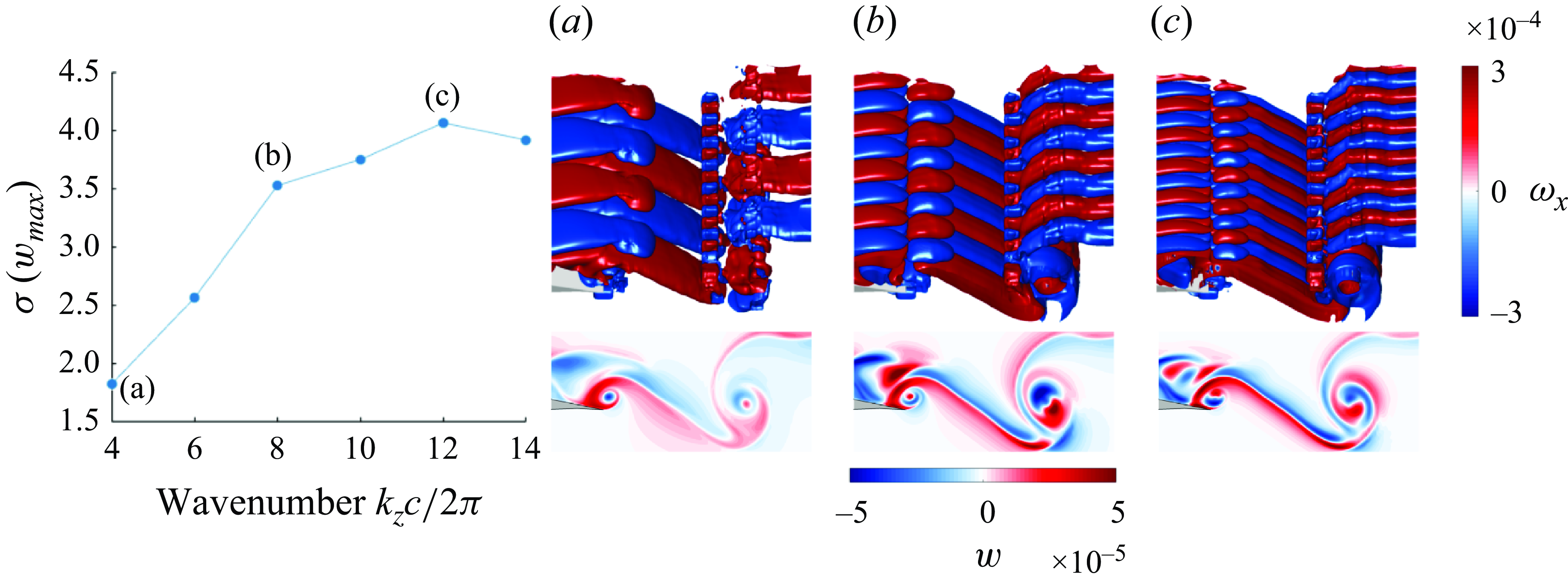
Figure 13. Left: temporal growth rate of
 $w_{max}$
for
$w_{max}$
for
 $\alpha$
= 6
$\alpha$
= 6
 $^{\circ }$
. Top right: iso-
$^{\circ }$
. Top right: iso-
 $\omega _x$
surfaces for wavenumbers 4 (a), 8 (b) and 12 (c) at
$\omega _x$
surfaces for wavenumbers 4 (a), 8 (b) and 12 (c) at
 $t$
= 1.0. Bottom right: corresponding contours of
$t$
= 1.0. Bottom right: corresponding contours of
 $w$
.
$w$
.
The spatio-temporal development of the perturbation is given in figure 14 for
 $\alpha$
= 4
$\alpha$
= 4
 $^{\circ }$
, where slices of the perturbation vorticity (
$^{\circ }$
, where slices of the perturbation vorticity (
 $\omega _x$
) are plotted for different perturbation wavenumbers at two instances in time, separated by one shedding period
$\omega _x$
) are plotted for different perturbation wavenumbers at two instances in time, separated by one shedding period
 $T$
. At
$T$
. At
 $k_z c/2\pi$
= 8 and 12, the vorticity changes its sign within the braids over one period, further corroborating the existence of a mode C (Gupta et al. Reference Gupta, Zhao, Sharma, Agrawal, Hourigan and Thompson2022). This change in the sign of
$k_z c/2\pi$
= 8 and 12, the vorticity changes its sign within the braids over one period, further corroborating the existence of a mode C (Gupta et al. Reference Gupta, Zhao, Sharma, Agrawal, Hourigan and Thompson2022). This change in the sign of
 $\omega _x$
does not occur at
$\omega _x$
does not occur at
 $k_z c/2\pi$
= 4. Therefore, it closely fits the shape of a mode A instability, which occurs at a lower growth rate (see figure 12).
$k_z c/2\pi$
= 4. Therefore, it closely fits the shape of a mode A instability, which occurs at a lower growth rate (see figure 12).
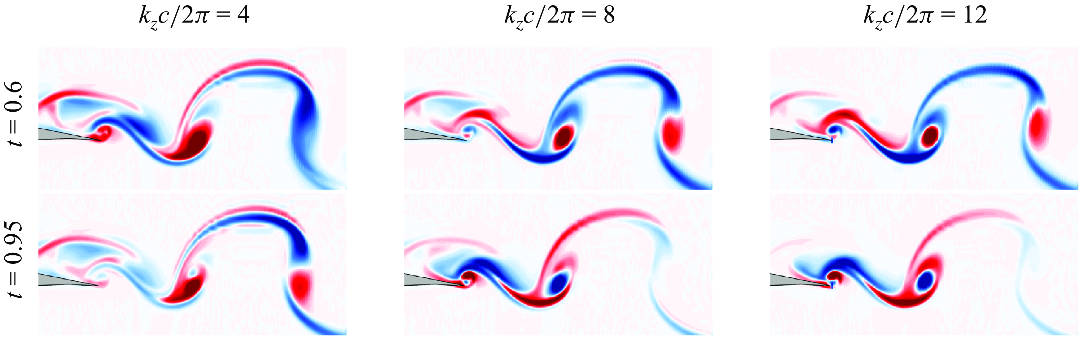
Figure 14. Contours of perturbation vorticity
 $\omega _x$
. Here,
$\omega _x$
. Here,
 $\alpha$
= 4
$\alpha$
= 4
 $^{\circ }$
.
$^{\circ }$
.
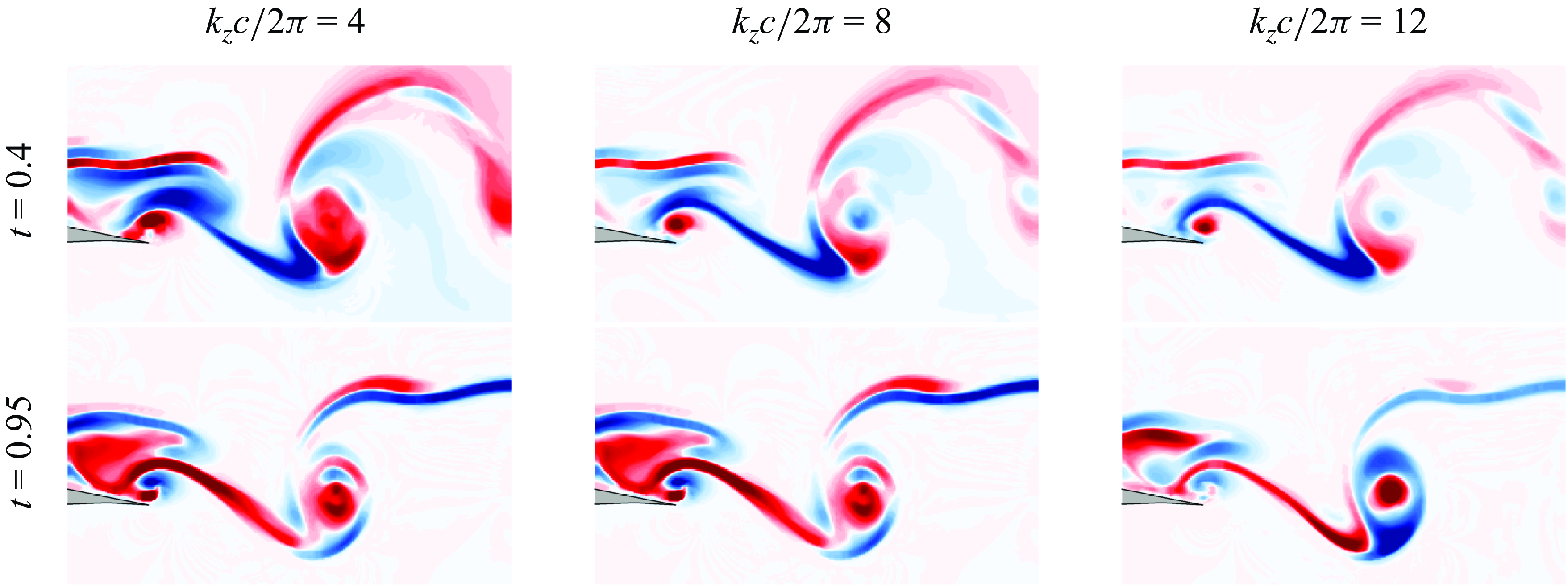
Figure 15. Contours of perturbation vorticity
 $\omega _x$
. Here,
$\omega _x$
. Here,
 $\alpha$
= 6
$\alpha$
= 6
 $^{\circ }$
.
$^{\circ }$
.
At
 $\alpha$
= 6
$\alpha$
= 6
 $^{\circ }$
(figure 15), the wake pattern is not quite symmetric over one shedding period, but a change in the sign of the perturbation vorticity
$^{\circ }$
(figure 15), the wake pattern is not quite symmetric over one shedding period, but a change in the sign of the perturbation vorticity
 $\omega _x$
within the braids occurs at all shown perturbation wavenumbers 4
$\omega _x$
within the braids occurs at all shown perturbation wavenumbers 4
 $\leqslant$
 $k_z c/2\pi$
 $\leqslant$
12, supporting the mode C instability, although being less distinct than at the lower angle of attack at
$\leqslant$
12, supporting the mode C instability, although being less distinct than at the lower angle of attack at
 $\alpha$
= 4
$\alpha$
= 4
 $^{\circ }$
.
$^{\circ }$
.
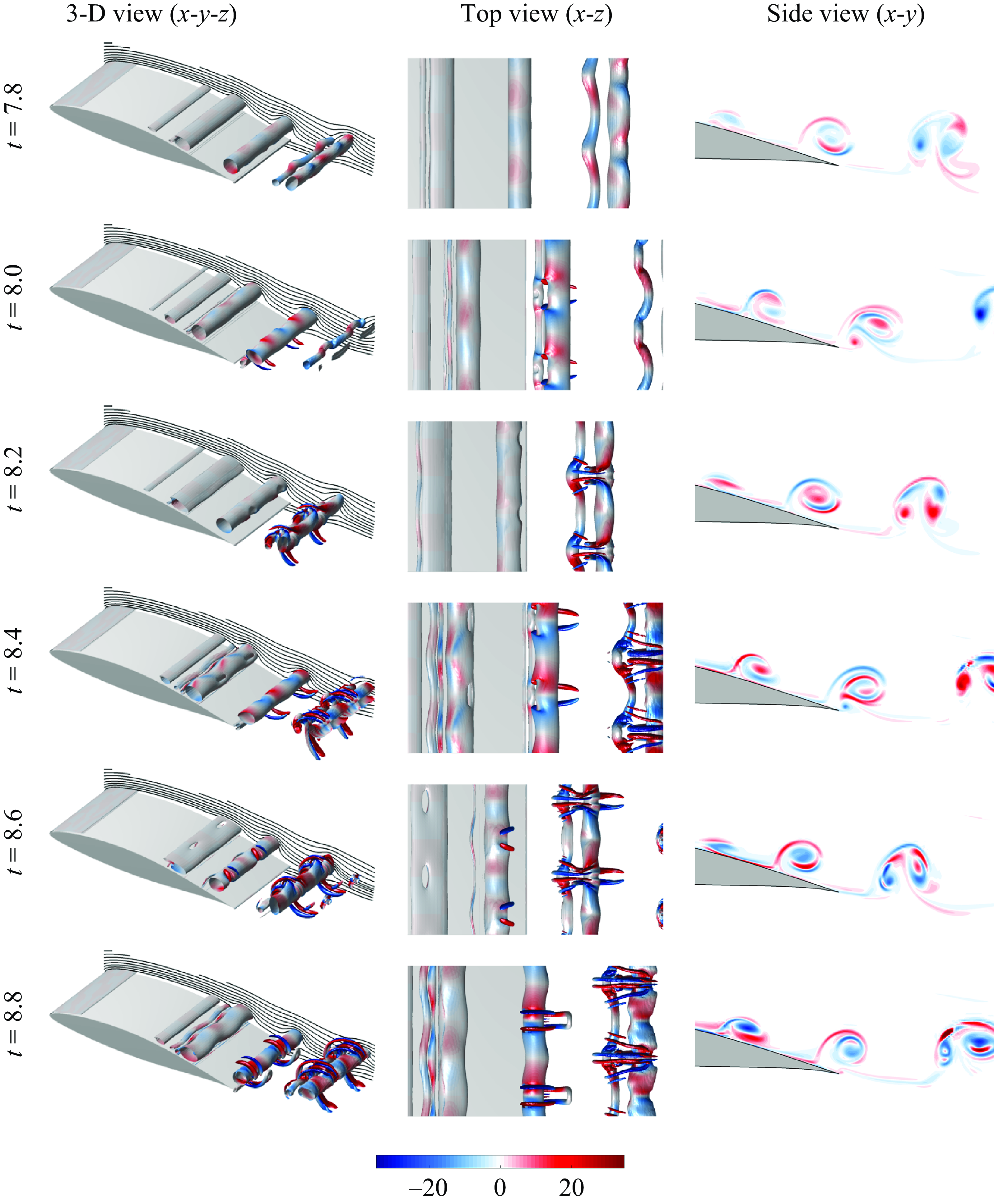
Figure 16. First two columns: iso-surfaces of
 $Q$
-criterion (level: 100) coloured by streamwise vorticity from
$Q$
-criterion (level: 100) coloured by streamwise vorticity from
 $t$
= 7.8 to
$t$
= 7.8 to
 $t$
= 8.8. Instantaneous streamlines in black. Third column: contours of streamwise vorticity
$t$
= 8.8. Instantaneous streamlines in black. Third column: contours of streamwise vorticity
 $\omega _x$
at
$\omega _x$
at
 $z/c$
= 0.25. Here,
$z/c$
= 0.25. Here,
 $\alpha$
= 7
$\alpha$
= 7
 $^{\circ }$
.
$^{\circ }$
.
4.3.3. Development of instabilities at
$\alpha _{\textit{crit}}$

The flow at angles of attack greater than the critical angle,
 $\alpha _{\textit{crit}}$
, is characterised by the formation of a closed and thin LSB and subsequent transition to turbulence. Assessing the natural development of 3-D flow structures from an initially 2-D state (i.e. without external forcing or perturbations to accelerate transition) enables us to pinpoint the instability mechanism directly. The development of 3-D instabilities is visualised in the series of snapshots from
$\alpha _{\textit{crit}}$
, is characterised by the formation of a closed and thin LSB and subsequent transition to turbulence. Assessing the natural development of 3-D flow structures from an initially 2-D state (i.e. without external forcing or perturbations to accelerate transition) enables us to pinpoint the instability mechanism directly. The development of 3-D instabilities is visualised in the series of snapshots from
 $t$
= 7.8 to
$t$
= 7.8 to
 $t$
= 8.8 in figure 16, where iso-surfaces of
$t$
= 8.8 in figure 16, where iso-surfaces of
 $Q$
coloured by the streamwise vorticity component
$Q$
coloured by the streamwise vorticity component
 $\omega _x$
show the emergence of 3-D modes within the vortices. Note that no perturbation or forcing is added to the flow and the transition occurs naturally. The flow is initially quasi-two-dimensional and characterised by the formation of spanwise KH vortices from the separating shear layer at mid-chord, which shed off the trailing edge and thereby form a pair of counter-rotating vortices. A well-defined low-frequency perturbation mode along the vortex at the trailing edge, as well as within the advected vortex pair downstream in the near wake, is made visible by the
$\omega _x$
show the emergence of 3-D modes within the vortices. Note that no perturbation or forcing is added to the flow and the transition occurs naturally. The flow is initially quasi-two-dimensional and characterised by the formation of spanwise KH vortices from the separating shear layer at mid-chord, which shed off the trailing edge and thereby form a pair of counter-rotating vortices. A well-defined low-frequency perturbation mode along the vortex at the trailing edge, as well as within the advected vortex pair downstream in the near wake, is made visible by the
 $\omega _x$
-velocity colouring at
$\omega _x$
-velocity colouring at
 $t$
= 7.8. The smaller of the two downstream vortices has attained noticeable bends with a wavelength of
$t$
= 7.8. The smaller of the two downstream vortices has attained noticeable bends with a wavelength of
 $\lambda _z/c$
= 0.25 whereas the larger tube is only weakly bulging along the span. This process repeats but with a phase-shifted spanwise modulation by
$\lambda _z/c$
= 0.25 whereas the larger tube is only weakly bulging along the span. This process repeats but with a phase-shifted spanwise modulation by
 $\lambda _z/2$
. This is also visible in the contour plots in the third column of figure 16, where the sign of
$\lambda _z/2$
. This is also visible in the contour plots in the third column of figure 16, where the sign of
 $\omega _x$
within the enveloping changes at a period of two times the vortex shedding period, proving that the naturally developing 3-D instability is the subharmonic mode C (Deng et al. Reference Deng, Sun and Shao2017; Gupta et al. Reference Gupta, Zhao, Sharma, Agrawal, Hourigan and Thompson2022).
$\omega _x$
within the enveloping changes at a period of two times the vortex shedding period, proving that the naturally developing 3-D instability is the subharmonic mode C (Deng et al. Reference Deng, Sun and Shao2017; Gupta et al. Reference Gupta, Zhao, Sharma, Agrawal, Hourigan and Thompson2022).
In addition to the mode C instability, the development of 3-D structures can also be traced to the interaction of counter-rotating vortex pairs in the near wake. Consider the vortex pair highlighted at
 $t$
= 7.8 in figures 17(a)–17(b): the two vortices are isolated and of unequal strength with significant bending (of sinusoidal shape) of the weaker vortex while the larger, stronger vortex remains relatively unperturbed. Vortex displacements modes of this form can also be observed in a Crow instability for counter-rotating vortex pairs of unequal strength (Leweke et al. Reference Leweke, Le Dizès and Williamson2016), where the vortices deform through mutual induction of their strain fields (and hence show different amplitudes of deformation). The bulging of the larger vortex, however, points towards the existence of an elliptic instability of the vortex core itself.
$t$
= 7.8 in figures 17(a)–17(b): the two vortices are isolated and of unequal strength with significant bending (of sinusoidal shape) of the weaker vortex while the larger, stronger vortex remains relatively unperturbed. Vortex displacements modes of this form can also be observed in a Crow instability for counter-rotating vortex pairs of unequal strength (Leweke et al. Reference Leweke, Le Dizès and Williamson2016), where the vortices deform through mutual induction of their strain fields (and hence show different amplitudes of deformation). The bulging of the larger vortex, however, points towards the existence of an elliptic instability of the vortex core itself.
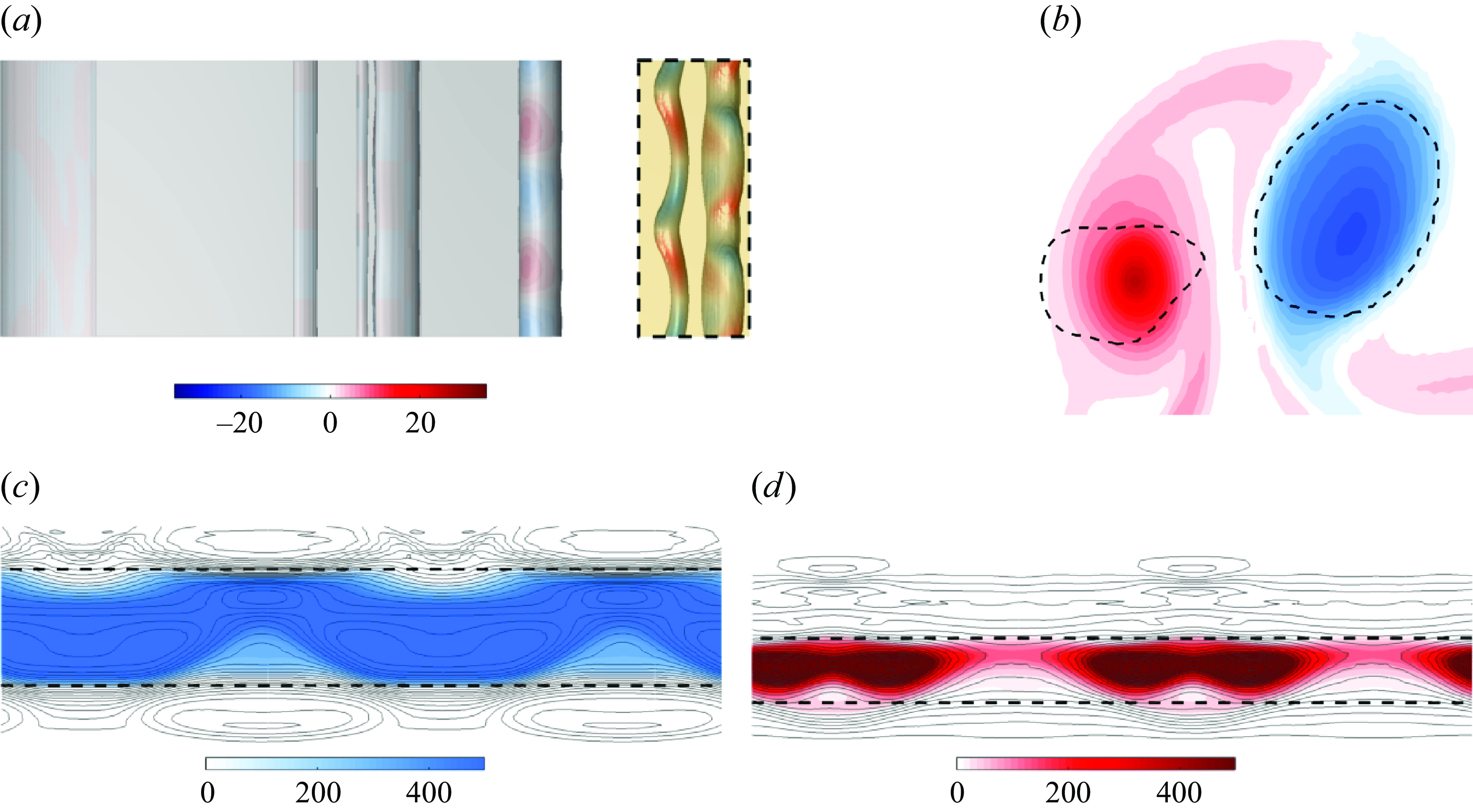
Figure 17. (a) Top view (
 $x$
-
$x$
-
 $z$
) of
$z$
) of
 $Q$
-criterion isosurfaces coloured by streamwise vorticity with highlighted vortex pair in near wake. (b) Side view (
$Q$
-criterion isosurfaces coloured by streamwise vorticity with highlighted vortex pair in near wake. (b) Side view (
 $x$
-
$x$
-
 $y$
) of spanwise vorticity contours of the highlighted vortex pair. Dashed lines indicated spanwise-averaged iso-
$y$
) of spanwise vorticity contours of the highlighted vortex pair. Dashed lines indicated spanwise-averaged iso-
 $Q$
contours. (c–d) Front view (
$Q$
contours. (c–d) Front view (
 $z$
–
$z$
–
 $y$
) of a slice through the vortex pair (c)
$y$
) of a slice through the vortex pair (c)
 $\omega _z\,\lt \,0,$
(d)
$\omega _z\,\lt \,0,$
(d)
 $\omega _z\,\gt \,0$
. Dashed lines are spanwise-averaged iso-lines of
$\omega _z\,\gt \,0$
. Dashed lines are spanwise-averaged iso-lines of
 $Q$
(level: 8). Here,
$Q$
(level: 8). Here,
 $\alpha \,=\,7^{\circ }$
at
$\alpha \,=\,7^{\circ }$
at
 $t\,=\,7.8$
.
$t\,=\,7.8$
.
Crow instabilities are generally considered vortex pair instabilities with the longest wavelengths and their growth rate depends on the ratio of circulation
 $\Lambda$
=
$\Lambda$
=
 $\Gamma _1 / \Gamma _2$
(
$\Gamma _1 / \Gamma _2$
(
 $\Gamma _1$
being the weaker vortex), the spacing between the cores
$\Gamma _1$
being the weaker vortex), the spacing between the cores
 $b$
and the vortex radius
$b$
and the vortex radius
 $a$
. The circulation is computed as
$a$
. The circulation is computed as
 \begin{equation} \Gamma = \int _S \mathbf {\omega } \mathrm {d}\mathbf {S}. \end{equation}
The determination of the vortex radius is, however, not straight forward, as there are different measures used in the literature. In the original works by Leweke & Williamson (Reference Leweke and Williamson1998a
) on instabilities of vortex pairs, the axial (spanwise in our case) perturbation wavelength of the vortex is mainly scaled with the diameter of the invariant streamtube
 $d_{\textit{inv}}$
. The fastest-growing wavelength of an elliptic instability, for example, was found to be
$d_{\textit{inv}}$
. The fastest-growing wavelength of an elliptic instability, for example, was found to be
 $\lambda _{\mathrm {e}}$
 $\approx$
4.0
$\approx$
4.0
 $d_{\textit{inv}}$
(Leweke & Williamson Reference Leweke and Williamson1998
Reference Leweke and Williamson
a
). Following Laporte & Corjon (Reference Laporte and Corjon2000), the invariant streamtube diameter can also be calculated from the invariant tube of axial vorticity, which is 40 % larger than
$d_{\textit{inv}}$
(Leweke & Williamson Reference Leweke and Williamson1998
Reference Leweke and Williamson
a
). Following Laporte & Corjon (Reference Laporte and Corjon2000), the invariant streamtube diameter can also be calculated from the invariant tube of axial vorticity, which is 40 % larger than
 $d_{\textit{inv}}$
. We apply this reasoning to the vortex pair in figure 17, where panels (c) and (d) show an axial slice of the two vortices. Iso-lines of the axial vorticity
$d_{\textit{inv}}$
. We apply this reasoning to the vortex pair in figure 17, where panels (c) and (d) show an axial slice of the two vortices. Iso-lines of the axial vorticity
 $\omega _z$
are given in grey and contours of the
$\omega _z$
are given in grey and contours of the
 $Q$
-criterion are in blue/red. In addition, we also indicate the region where the spanwise-averaged value of
$Q$
-criterion are in blue/red. In addition, we also indicate the region where the spanwise-averaged value of
 $Q$
is positive (>8 here to avoid artefacts from noise) by dashed lines. The plots show that spanwise-averaged
$Q$
is positive (>8 here to avoid artefacts from noise) by dashed lines. The plots show that spanwise-averaged
 $Q$
provides a reasonable estimate of the invariant tube of axial vorticity, i.e. it approximates the locations where the streamline remains unaffected by the inner perturbation (Leweke & Williamson Reference Leweke and Williamson1998
Reference Leweke and Williamson
a
). In the following, we will scale the vortex radius as
$Q$
provides a reasonable estimate of the invariant tube of axial vorticity, i.e. it approximates the locations where the streamline remains unaffected by the inner perturbation (Leweke & Williamson Reference Leweke and Williamson1998
Reference Leweke and Williamson
a
). In the following, we will scale the vortex radius as
 $a$
=
$a$
=
 $r_{Q\gt 0}/1.4$
, where
$r_{Q\gt 0}/1.4$
, where
 $r_{Q\gt 0}$
is the radius measured by the region
$r_{Q\gt 0}$
is the radius measured by the region
 $Q\gt 0$
shown in figure 17.
$Q\gt 0$
shown in figure 17.
The parameters of the vortex pair at
 $t\,=\,7.8$
(figure 17) are thus
$t\,=\,7.8$
(figure 17) are thus
 $\Lambda \,=\,-0.3, a_-\,=\,0.03c$
(vortex with
$\Lambda \,=\,-0.3, a_-\,=\,0.03c$
(vortex with
 $\Gamma \,\lt \,0$
),
$\Gamma \,\lt \,0$
),
 $a_+\,=\,0.02c$
(vortex with
$a_+\,=\,0.02c$
(vortex with
 $\Gamma \,\gt \,0$
),
$\Gamma \,\gt \,0$
),
 $a_+/b\,=\,0.21, k_z a_-\,=\,0.75$
,
$a_+/b\,=\,0.21, k_z a_-\,=\,0.75$
,
 $k_z a_+\,=\,0.5$
and
$k_z a_+\,=\,0.5$
and
 $\lambda _z/b\,=\,2.6$
. The wavenumber is
$\lambda _z/b\,=\,2.6$
. The wavenumber is
 $k_z\,=\,2\pi /\lambda _z$
. We note that near identical values can be calculated for the following vortex pair visible from
$k_z\,=\,2\pi /\lambda _z$
. We note that near identical values can be calculated for the following vortex pair visible from
 $t\,=\,$
8.0 to 8.4 in figure 16. While the Crow instability in vortex pairs of equal strength grows for spanwise perturbations of wavelengths in the range
$t\,=\,$
8.0 to 8.4 in figure 16. While the Crow instability in vortex pairs of equal strength grows for spanwise perturbations of wavelengths in the range
 $6b \leqslant \lambda _z \leqslant 10b$
, the wavelength can be as low as
$6b \leqslant \lambda _z \leqslant 10b$
, the wavelength can be as low as
 $\lambda _z\,\approx \,b$
for pairs of unequal strength (Leweke et al. Reference Leweke, Le Dizès and Williamson2016). For such unequal-strength vortices, as is the case here, So, Ryan & Sheard (Reference So, Ryan and Sheard2011) reported peaks in the growth rate of the Crow instability between
$\lambda _z\,\approx \,b$
for pairs of unequal strength (Leweke et al. Reference Leweke, Le Dizès and Williamson2016). For such unequal-strength vortices, as is the case here, So, Ryan & Sheard (Reference So, Ryan and Sheard2011) reported peaks in the growth rate of the Crow instability between
 $k_z a\,=\,0.1 (\Lambda \,=\,-0.9)$
and
$k_z a\,=\,0.1 (\Lambda \,=\,-0.9)$
and
 $k_z a\approx \,1$
for
$k_z a\approx \,1$
for
 $\Lambda \,=\,-0.3$
. Similar values are reported by Ryan, Butler & Sheard (Reference Ryan, Butler and Sheard2012), who reported a critical wavenumber of
$\Lambda \,=\,-0.3$
. Similar values are reported by Ryan, Butler & Sheard (Reference Ryan, Butler and Sheard2012), who reported a critical wavenumber of
 $k_z a\,=\,0.75$
for
$k_z a\,=\,0.75$
for
 $\Lambda \,=\,-0.5$
. These values match our measurements of
$\Lambda \,=\,-0.5$
. These values match our measurements of
 $0.5\,\leqslant \,k_z a\,\leqslant \,0.75$
well and we conclude that the Crow instability mechanism plays a crucial role in the initial development of the instabilities and the transition in this flow.
$0.5\,\leqslant \,k_z a\,\leqslant \,0.75$
well and we conclude that the Crow instability mechanism plays a crucial role in the initial development of the instabilities and the transition in this flow.
While the sinusoidal shape of the weaker vortex and its scalings point to a Crow-type instability, the initial bulging of the stronger vortex, as well as the internal shape of the streamtube pattern givenin figure 17(c) match the form of an elliptic instability well (Laporte & Corjon Reference Laporte and Corjon2000). As noted by many authors (Leweke & Williamson Reference Leweke and Williamson1998
Reference Leweke and Williamson
a
; Laporte & Corjon Reference Laporte and Corjon2000; Ryan et al. Reference Ryan, Butler and Sheard2012; Leweke et al. Reference Leweke, Le Dizès and Williamson2016), elliptic and Crow instabilities often occur together and result in the emergence of secondary vortices and an increased breakdown rate. The non-dimensional wavenumber of the stronger vortex
 $k_z a_-\,=\,0.75$
is, however, significantly smaller than the predicted value of
$k_z a_-\,=\,0.75$
is, however, significantly smaller than the predicted value of
 $k_{z} a\,=\,1.6$
(or
$k_{z} a\,=\,1.6$
(or
 $\lambda _z\,=\,2d_{\textit{inv}}$
) for an elliptic instability (Leweke & Williamson Reference Leweke and Williamson1998
Reference Leweke and Williamson
a
; Laporte & Corjon Reference Laporte and Corjon2000), although values of
$\lambda _z\,=\,2d_{\textit{inv}}$
) for an elliptic instability (Leweke & Williamson Reference Leweke and Williamson1998
Reference Leweke and Williamson
a
; Laporte & Corjon Reference Laporte and Corjon2000), although values of
 $\lambda _z\,=\,\approx \,3D\,\approx \,3d_{\textit{core}}$
have also been reported by the authors (Leweke & Williamson Reference Leweke and Williamson1998
Reference Leweke and Williamson
b
) for the wake transition behind a cylinder of diameter
$\lambda _z\,=\,\approx \,3D\,\approx \,3d_{\textit{core}}$
have also been reported by the authors (Leweke & Williamson Reference Leweke and Williamson1998
Reference Leweke and Williamson
b
) for the wake transition behind a cylinder of diameter
 $D$
. If we scale the spanwise wavelength with the diameter measure by
$D$
. If we scale the spanwise wavelength with the diameter measure by
 $d_{Q\gt 0}$
(see figure 17
c), a very similar value of
$d_{Q\gt 0}$
(see figure 17
c), a very similar value of
 $\lambda _z/d_{Q\gt 0}\,=\,3.1$
can be obtained. It is therefore likely that both elliptic and Crow instability mechanisms are combined here (with the elliptic instability likely occurring first and inducing the initial perturbation) and result in the spanwise vortex deformations and later the emergence of secondary braids and
$\lambda _z/d_{Q\gt 0}\,=\,3.1$
can be obtained. It is therefore likely that both elliptic and Crow instability mechanisms are combined here (with the elliptic instability likely occurring first and inducing the initial perturbation) and result in the spanwise vortex deformations and later the emergence of secondary braids and
 $\Omega$
-loops that transition the flow to turbulence.
$\Omega$
-loops that transition the flow to turbulence.
As the time series in figure 16 shows, the flow perturbations are gradually established over the airfoil’s suction side and notably deform the KH vortices upstream of the trailing edge at
 $t\,=\,8.8$
. To monitor the development of the 3-D instability over the airfoil surface, we consider a time series of streamwise vorticity iso-surfaces
$t\,=\,8.8$
. To monitor the development of the 3-D instability over the airfoil surface, we consider a time series of streamwise vorticity iso-surfaces
 $|\omega _x|$
= 1 in figure 18. The vortical structures identified in this way only relate to rotating fluid along the streamwise axis and hence detect 3-D flow patterns without being obscured by the dominating 2-D topology. The
$|\omega _x|$
= 1 in figure 18. The vortical structures identified in this way only relate to rotating fluid along the streamwise axis and hence detect 3-D flow patterns without being obscured by the dominating 2-D topology. The
 $\omega _x$
surfaces in figure 18 are flat layers that are stacked on the airfoil surface and lifted off by passing spanwise vortices. A similar topology of streamwise vorticity surfaces has been reported by Jones et al. (Reference Jones, Sandberg and Sandham2008) for the LSB shedding over a NACA 0012 and by Sakai, Diamessis & Jacobs (Reference Sakai, Diamessis and Jacobs2020) for the instability of a LSB under a solitary wave.
$\omega _x$
surfaces in figure 18 are flat layers that are stacked on the airfoil surface and lifted off by passing spanwise vortices. A similar topology of streamwise vorticity surfaces has been reported by Jones et al. (Reference Jones, Sandberg and Sandham2008) for the LSB shedding over a NACA 0012 and by Sakai, Diamessis & Jacobs (Reference Sakai, Diamessis and Jacobs2020) for the instability of a LSB under a solitary wave.
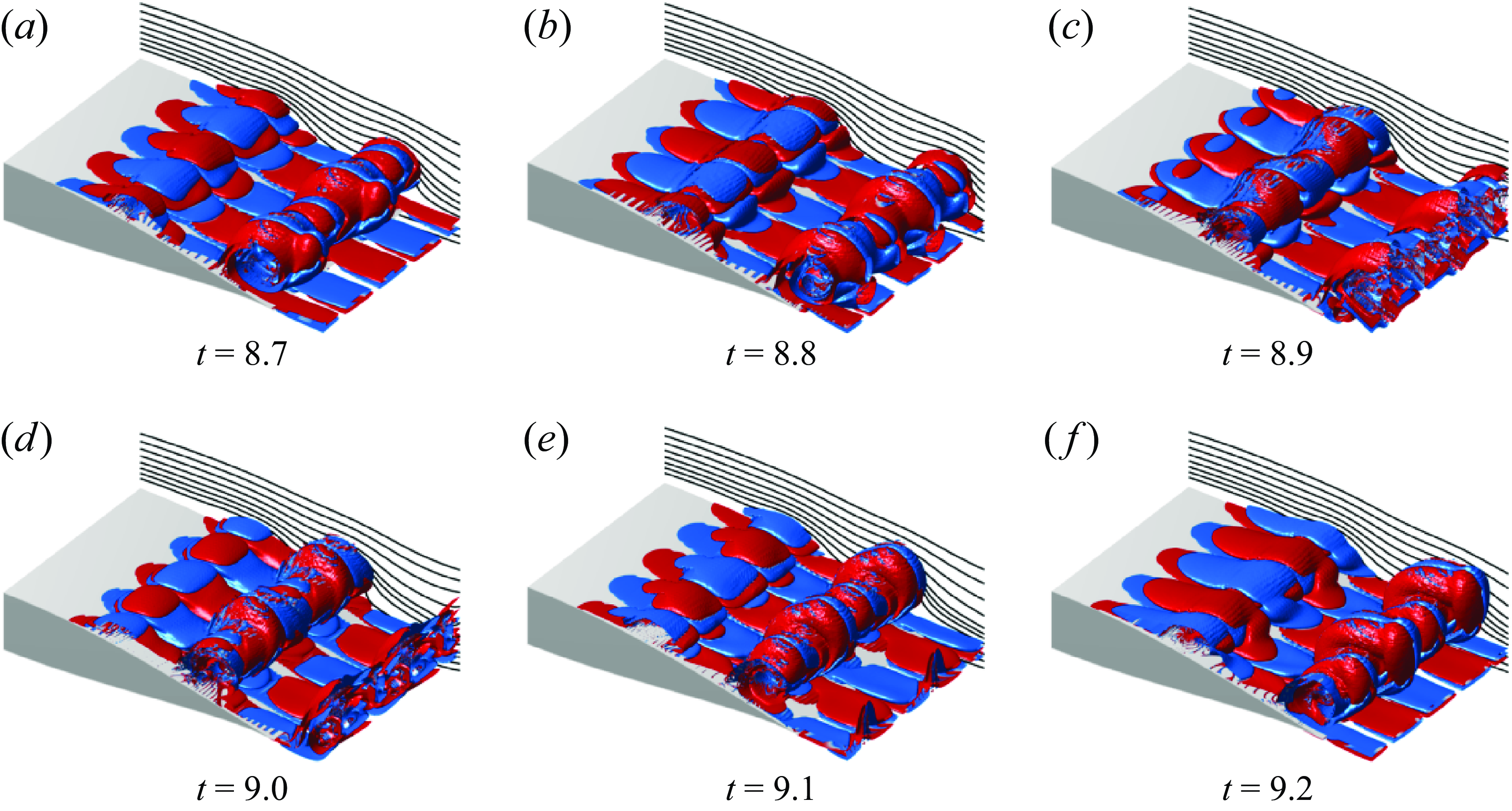
Figure 18. Iso-surfaces of the streamwise vorticity
 $+\omega _x$
(red) and
$+\omega _x$
(red) and
 $-\omega _x$
(blue) for a level
$-\omega _x$
(blue) for a level
 $|\omega _x|$
= 1. Rear section of the airfoil shown between
$|\omega _x|$
= 1. Rear section of the airfoil shown between
 $x/c$
= 0.4 and
$x/c$
= 0.4 and
 $x/c$
= 1.1 for
$x/c$
= 1.1 for
 $t$
= 8.7 (a) to
$t$
= 8.7 (a) to
 $t$
= 9.2 (f). Instantaneous streamlines in black. Here,
$t$
= 9.2 (f). Instantaneous streamlines in black. Here,
 $\alpha$
= 7
$\alpha$
= 7
 $^{\circ }$
.
$^{\circ }$
.
The time series in figure 18 illustrates that streamwise vorticity is present within a thin layer at the trailing edge in a slender region of recirculating fluid (bubble height = 0.026
 $c$
). As the next vortex forms, it is bent by the existing rotating flow near the airfoil surface and, as the vortex line tilts, induces streamwise vorticity itself, thereby amplifying the spanwise velocity component. The cycle repeats until the bending of the spanwise vortices towards the trailing edge at a location where patches of positive and negative
$c$
). As the next vortex forms, it is bent by the existing rotating flow near the airfoil surface and, as the vortex line tilts, induces streamwise vorticity itself, thereby amplifying the spanwise velocity component. The cycle repeats until the bending of the spanwise vortices towards the trailing edge at a location where patches of positive and negative
 $\omega _x$
induce a wall-normal upwelling fluid movement (see figure 18
f). The iso-surfaces of
$\omega _x$
induce a wall-normal upwelling fluid movement (see figure 18
f). The iso-surfaces of
 $Q$
shown in figure 19(b)–(c) indicate that this asymmetric bending is associated with the generation of loop vortices that eventually grow into the enveloping braids at later times.
$Q$
shown in figure 19(b)–(c) indicate that this asymmetric bending is associated with the generation of loop vortices that eventually grow into the enveloping braids at later times.
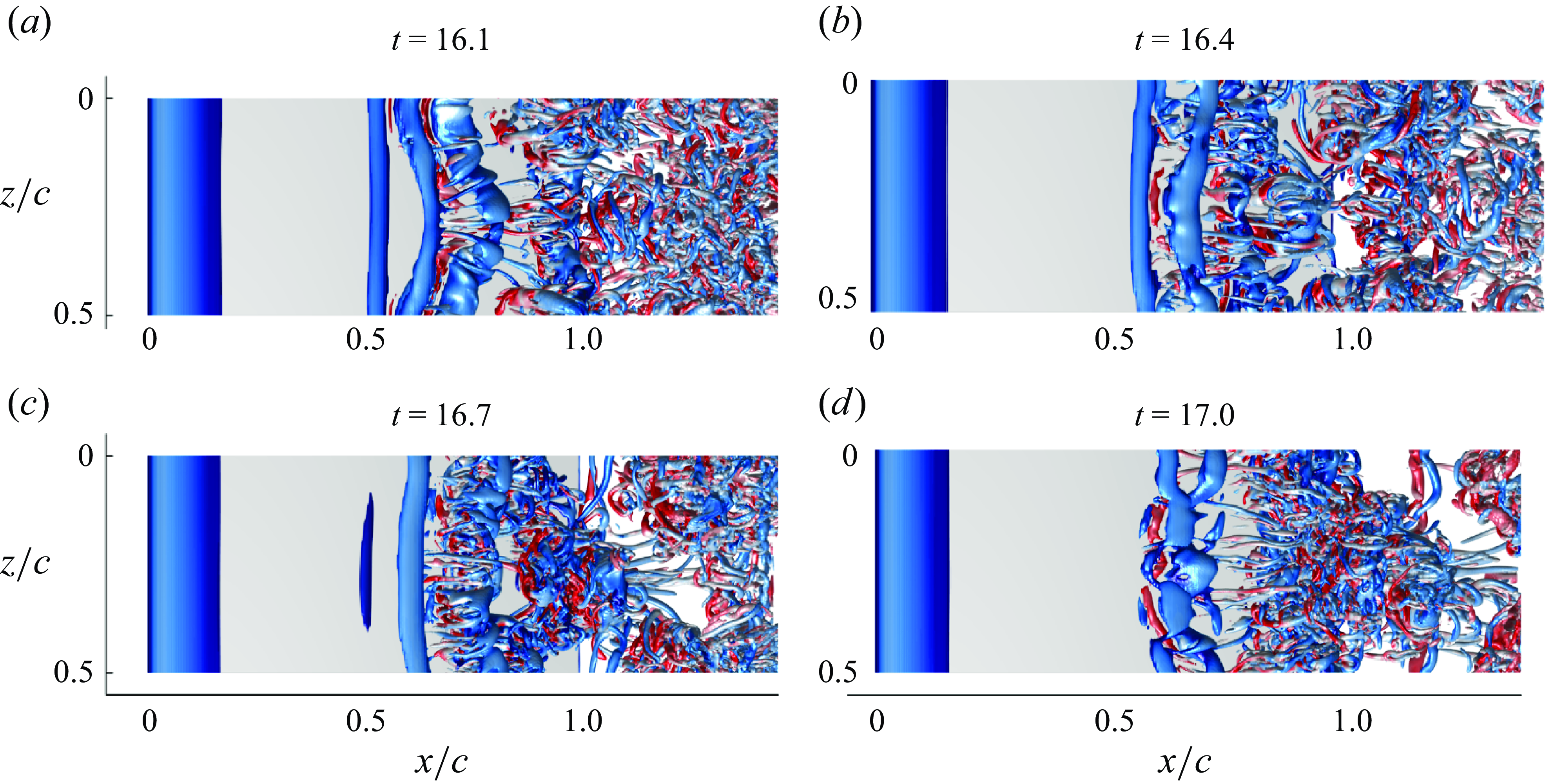
Figure 19. Iso-
 $Q$
surfaces for
$Q$
surfaces for
 $\alpha$
= 7
$\alpha$
= 7
 $^{\circ }$
at
$^{\circ }$
at
 $t$
= 16.3 (a), 16.5 (b), 16.7 (c) and 16.9 (d). Colouring by spanwise vorticity
$t$
= 16.3 (a), 16.5 (b), 16.7 (c) and 16.9 (d). Colouring by spanwise vorticity
 $\omega _z$
.
$\omega _z$
.
Crow–KH interactions
Low-frequency spanwise modes within the KH vortices are also present at later times and drive the formation of large-scale turbulent structures. At
 $t$
$t$
 $\approx$
16, the bending of spanwise vortices results in a horseshoe-type vortex structure that extends over the span of the airfoil and bursts into a turbulent cloud or ‘puff’. The process is outlined in figure 19 and starts with the bending of the KH vortex along the span in streamwise direction (figure 19
a).
$\approx$
16, the bending of spanwise vortices results in a horseshoe-type vortex structure that extends over the span of the airfoil and bursts into a turbulent cloud or ‘puff’. The process is outlined in figure 19 and starts with the bending of the KH vortex along the span in streamwise direction (figure 19
a).
While the nominally 2-D flow structure breaks down and forms smaller-scale loop vortices (figure 19
b), a large-scale coherent horseshoe-shaped vortex system develops (figure 19
c), which then bursts and sheds off at the trailing edge (figure 19
d). Because the wavelength of this mode (
 $\lambda _z$
= 0.5
$\lambda _z$
= 0.5
 $c$
) is twice the expected wavelength of an elliptic instability for the given vortex diameter (
$c$
) is twice the expected wavelength of an elliptic instability for the given vortex diameter (
 $d_{\textit{core}}$
 $\approx$
0.06), the large-scale deformation of the KH vortex in figure 19(a) is at least partly the result of the interaction with downstream vortices through induction of velocity in the upstream vortices (Crow-type instability). The series in figure 19(a–d) shows how the interplay of 3-D large-scale instability modes and the small-scale loop vortices results in the formation and bursting of such large coherent turbulent structures.
$\approx$
0.06), the large-scale deformation of the KH vortex in figure 19(a) is at least partly the result of the interaction with downstream vortices through induction of velocity in the upstream vortices (Crow-type instability). The series in figure 19(a–d) shows how the interplay of 3-D large-scale instability modes and the small-scale loop vortices results in the formation and bursting of such large coherent turbulent structures.
4.3.4. The case of SII - high
$\alpha$

As the impact of the elliptic instability grows with increasing
 $\alpha$
from 0
$\alpha$
from 0
 $^{\circ }$
to 7
$^{\circ }$
to 7
 $^{\circ }$
, the flow structures are less distinct within the LSB located near the leading edge at
$^{\circ }$
, the flow structures are less distinct within the LSB located near the leading edge at
 $\alpha$
= 8
$\alpha$
= 8
 $^{\circ }$
. Figure 20 shows a top (suction-side) view of the vortical structures at
$^{\circ }$
. Figure 20 shows a top (suction-side) view of the vortical structures at
 $\alpha$
= 8
$\alpha$
= 8
 $^{\circ }$
and 10
$^{\circ }$
and 10
 $^{\circ }$
. It is observed that the separated laminar shear layer sheds KH vortices which break down before mid-chord and loose their spatial coherence as the flow transitions to a turbulent boundary layer. Non-zero spanwise velocity and 3-D vortex structures are also present throughout the upstream, laminar section of the bubble and result in the non-uniform generation of the KH vortices with vortex displacements and re-connections visible. Low-frequency deformations of the KH vortices and the generation of hairpin loops within the shear region point to the same instability mechanisms observed at lower
$^{\circ }$
. It is observed that the separated laminar shear layer sheds KH vortices which break down before mid-chord and loose their spatial coherence as the flow transitions to a turbulent boundary layer. Non-zero spanwise velocity and 3-D vortex structures are also present throughout the upstream, laminar section of the bubble and result in the non-uniform generation of the KH vortices with vortex displacements and re-connections visible. Low-frequency deformations of the KH vortices and the generation of hairpin loops within the shear region point to the same instability mechanisms observed at lower
 $\alpha$
, but their occurrence is less pronounced and masked by the rapid transition to turbulence.
$\alpha$
, but their occurrence is less pronounced and masked by the rapid transition to turbulence.
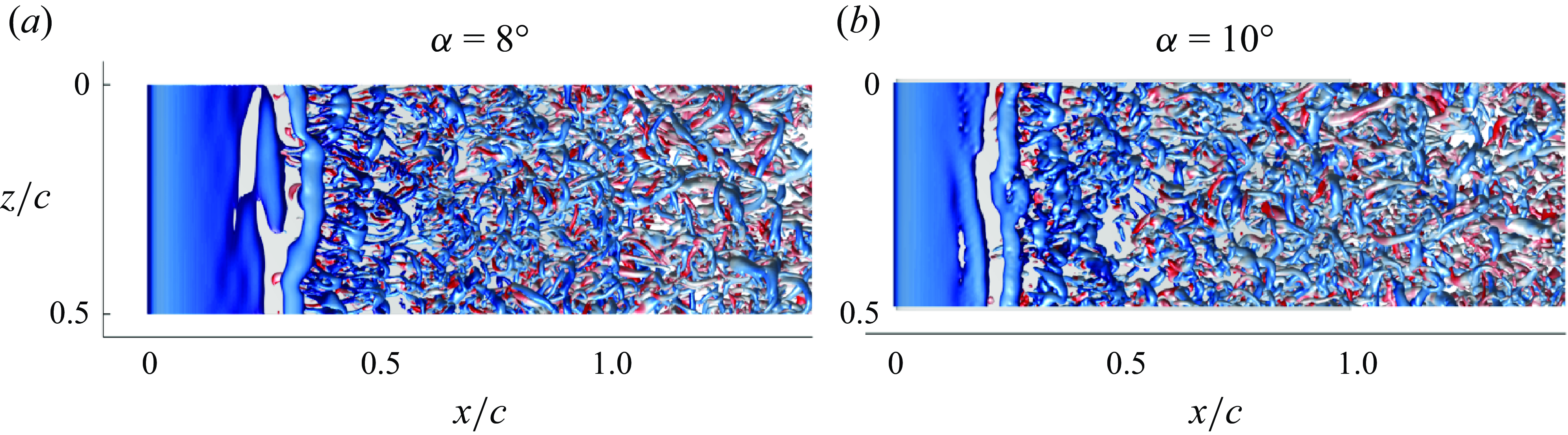
Figure 20. Iso-
 $Q$
surfaces for
$Q$
surfaces for
 $\alpha$
= 8
$\alpha$
= 8
 $^{\circ }$
(a) and 10
$^{\circ }$
(a) and 10
 $^{\circ }$
. Colouring by spanwise vorticity
$^{\circ }$
. Colouring by spanwise vorticity
 $\omega _z$
.
$\omega _z$
.
4.3.5. The footprint of flow instabilities in unsteady forces
Figure 21 shows the time history of the lift and drag coefficients, as well as the corresponding frequency spectrum for the flow at
 $\alpha$
= 0
$\alpha$
= 0
 $^{\circ }$
, 4
$^{\circ }$
, 4
 $^{\circ }$
, 7
$^{\circ }$
, 7
 $^{\circ }$
and 8
$^{\circ }$
and 8
 $^{\circ }$
. The time unit is scaled with the free-stream velocity
$^{\circ }$
. The time unit is scaled with the free-stream velocity
 $U_\infty$
and the chord-length of the airfoil
$U_\infty$
and the chord-length of the airfoil
 $c$
, so the corresponding frequency is a Strouhal number St =
$c$
, so the corresponding frequency is a Strouhal number St =
 $fc/U_\infty$
.
$fc/U_\infty$
.
At the lower
 $\alpha$
(0
$\alpha$
(0
 $^{\circ }$
and 4
$^{\circ }$
and 4
 $^{\circ }$
), the oscillations of the forces are regular and driven by the shedding of the Kármán vortices from the laminar shear layers at the trailing edge that result in the narrow wakes presented in figure 22.
$^{\circ }$
), the oscillations of the forces are regular and driven by the shedding of the Kármán vortices from the laminar shear layers at the trailing edge that result in the narrow wakes presented in figure 22.
At
 $\alpha$
= 0
$\alpha$
= 0
 $^{\circ }$
, the lift coefficient spectrum has a distinct, single peak at a Strouhal number of St = 3.1, indicating that Kármán shedding determines the temporal flow development and no secondary instabilities exist. The increasingly unstable separated shear layer at higher angles results in additional low-frequency content in the lift spectrum at
$^{\circ }$
, the lift coefficient spectrum has a distinct, single peak at a Strouhal number of St = 3.1, indicating that Kármán shedding determines the temporal flow development and no secondary instabilities exist. The increasingly unstable separated shear layer at higher angles results in additional low-frequency content in the lift spectrum at
 $\alpha$
= 4
$\alpha$
= 4
 $^{\circ }$
, which still shows a dominant peak (at St = 2.7), but at a reduced amplitude (by 15 %), an indication that energy is transferred to modes with other frequencies.
$^{\circ }$
, which still shows a dominant peak (at St = 2.7), but at a reduced amplitude (by 15 %), an indication that energy is transferred to modes with other frequencies.
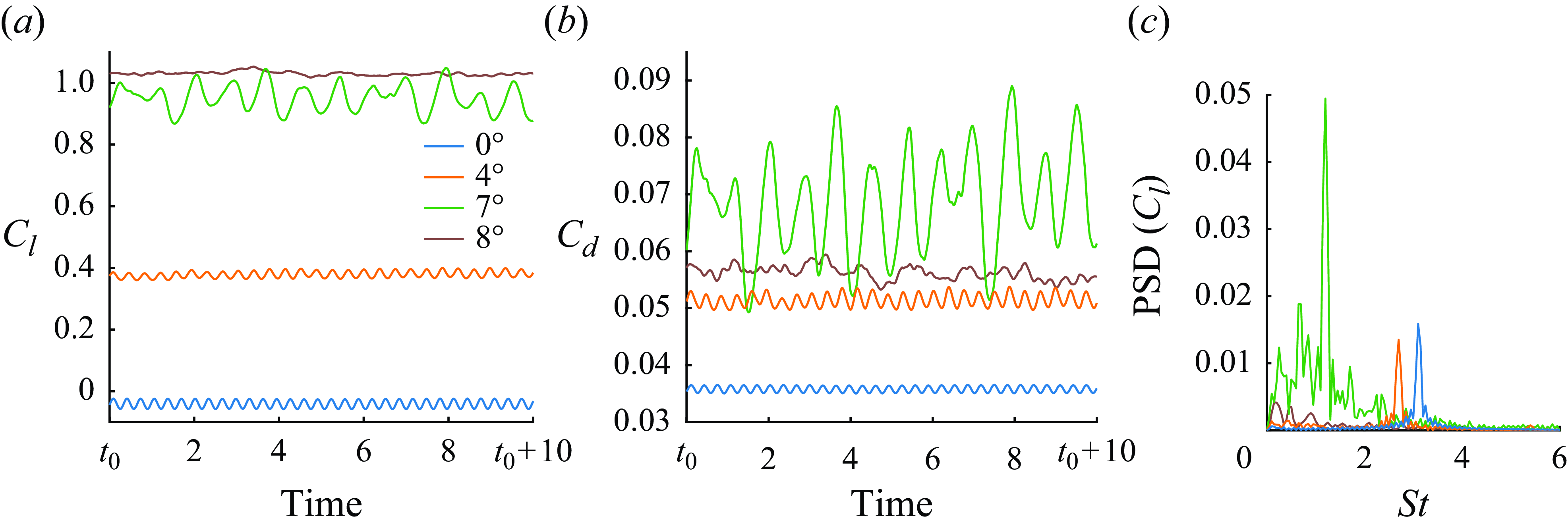
Figure 21. Lift (a) and drag (b) coefficients over time. (c) Frequency spectrum of the lift coefficient. For
 $\alpha$
= 0
$\alpha$
= 0
 $^{\circ }$
, 4
$^{\circ }$
, 4
 $^{\circ }$
, 7
$^{\circ }$
, 7
 $^{\circ }$
and 8
$^{\circ }$
and 8
 $^{\circ }$
.
$^{\circ }$
.
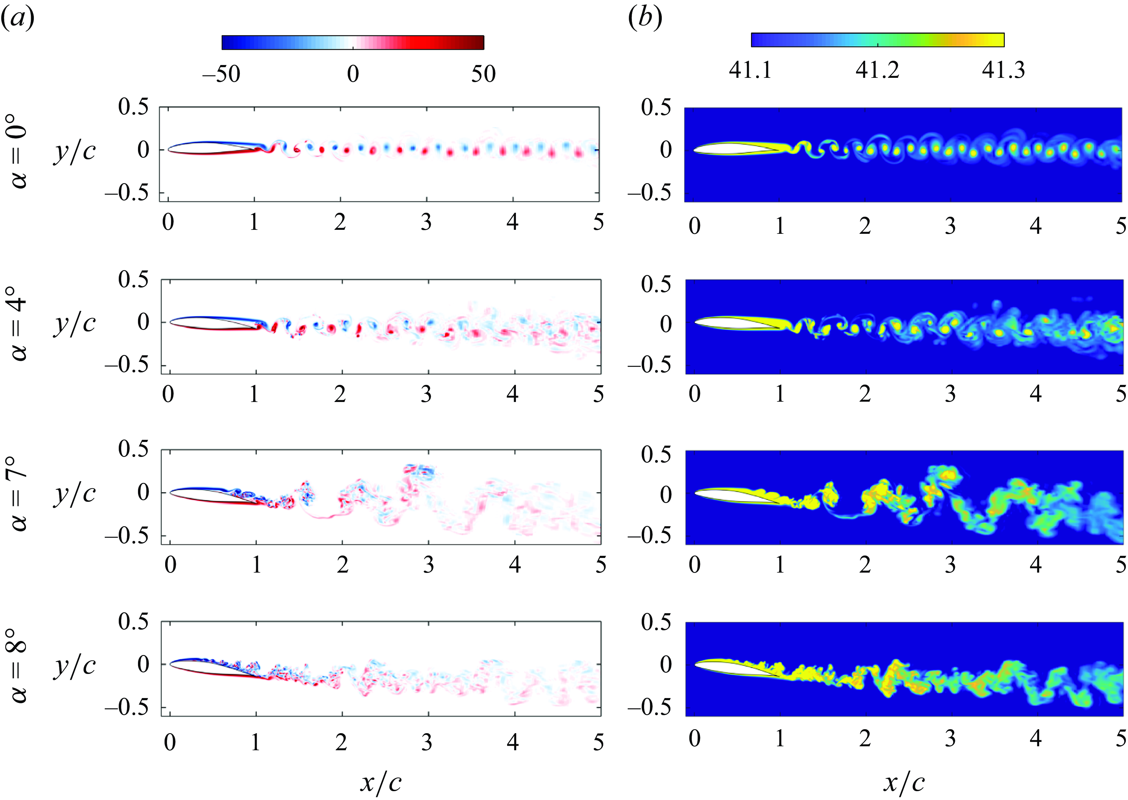
Figure 22. Instantaneous snapshots of the vorticity
 $\omega _z$
(a) and the specific entropy
$\omega _z$
(a) and the specific entropy
 $s$
=
$s$
=
 $\ln (p/\rho ^\gamma)/(\gamma (\gamma -1)M_f^2)$
(b) along a slice at
$\ln (p/\rho ^\gamma)/(\gamma (\gamma -1)M_f^2)$
(b) along a slice at
 $z/c$
= 0.025 for
$z/c$
= 0.025 for
 $\alpha$
= 0
$\alpha$
= 0
 $^{\circ }$
, 4
$^{\circ }$
, 4
 $^{\circ }$
, 7
$^{\circ }$
, 7
 $^{\circ }$
and 8
$^{\circ }$
and 8
 $^{\circ }$
(top to bottom).
$^{\circ }$
(top to bottom).
At
 $\alpha$
= 7
$\alpha$
= 7
 $^{\circ }$
and 8
$^{\circ }$
and 8
 $^{\circ }$
, the force oscillations are irregular and strongly dependent on the location of the LSB. If the LSB forms at the trailing edge of the airfoil (
$^{\circ }$
, the force oscillations are irregular and strongly dependent on the location of the LSB. If the LSB forms at the trailing edge of the airfoil (
 $\alpha$
= 7
$\alpha$
= 7
 $^{\circ }$
), then the interaction between instabilities on the suction side (KH shedding) and pressure side (Kármán shedding) result in large-scale turbulent bursts and large-amplitude oscillations of the aerodynamic forces (figure 21
a,b). The corresponding lift spectrum shows a dominant peak at St = 1.2 with an amplitude that is more than twice the amplitude as compared with the maxima at
$^{\circ }$
), then the interaction between instabilities on the suction side (KH shedding) and pressure side (Kármán shedding) result in large-scale turbulent bursts and large-amplitude oscillations of the aerodynamic forces (figure 21
a,b). The corresponding lift spectrum shows a dominant peak at St = 1.2 with an amplitude that is more than twice the amplitude as compared with the maxima at
 $\alpha$
= 0
$\alpha$
= 0
 $^{\circ }$
or 4
$^{\circ }$
or 4
 $^{\circ }$
. Moreover, low-frequency peaks are observable at St = 0.3 and 0.8 that also have greater or equal amplitudes as the peak at
$^{\circ }$
. Moreover, low-frequency peaks are observable at St = 0.3 and 0.8 that also have greater or equal amplitudes as the peak at
 $\alpha$
= 4
$\alpha$
= 4
 $^{\circ }$
(figure 21
c). The high energy content of these fluctuations results from the interaction of both Kármán (pressure-side) and KH (suction-side) instabilities, whereas the shedding at 0
$^{\circ }$
(figure 21
c). The high energy content of these fluctuations results from the interaction of both Kármán (pressure-side) and KH (suction-side) instabilities, whereas the shedding at 0
 $^{\circ }$
and 4
$^{\circ }$
and 4
 $^{\circ }$
is mainly driven by the Kármán instability induced by the roll-up of the pressure-side shear layer. In the case of a leading-edge LSB (
$^{\circ }$
is mainly driven by the Kármán instability induced by the roll-up of the pressure-side shear layer. In the case of a leading-edge LSB (
 $\alpha$
= 8
$\alpha$
= 8
 $^{\circ }$
), the time-averaged lift force (
$^{\circ }$
), the time-averaged lift force (
 $\bar {C}_l$
= 1.03) is higher than at the other
$\bar {C}_l$
= 1.03) is higher than at the other
 $\alpha$
, but the amplitude of the oscillations is reduced (figure 21
a). The lift spectrum (figure 21
c) does not show a dominant shedding frequency, but has several low-frequency peaks at only a third of the amplitude computed for the other cases. The low-amplitude oscillations are caused by the break up of the KH vortices and the transition to a turbulent boundary layer at mid-chord, which increases the isotropy of the flow structures on the suction side and interrupts the pressure-side shear layer from rolling into a large vortex.
$\alpha$
, but the amplitude of the oscillations is reduced (figure 21
a). The lift spectrum (figure 21
c) does not show a dominant shedding frequency, but has several low-frequency peaks at only a third of the amplitude computed for the other cases. The low-amplitude oscillations are caused by the break up of the KH vortices and the transition to a turbulent boundary layer at mid-chord, which increases the isotropy of the flow structures on the suction side and interrupts the pressure-side shear layer from rolling into a large vortex.
4.3.6. The footprint of flow instabilities upon the wake
The spatial development of the vortex street in the airfoil wake is visualised in figure 22 for
 $\alpha$
= 0
$\alpha$
= 0
 $^{\circ }$
, 4
$^{\circ }$
, 4
 $^{\circ }$
, 7
$^{\circ }$
, 7
 $^{\circ }$
and 8
$^{\circ }$
and 8
 $^{\circ }$
, where contours of the instantaneous, spanwise vorticity component
$^{\circ }$
, where contours of the instantaneous, spanwise vorticity component
 $\omega _z$
are plotted in (a) and contours of the specific entropy
$\omega _z$
are plotted in (a) and contours of the specific entropy
 $s$
in (b). Vorticity is generated at the airfoil wall and transported downstream, where stretching of vortex filaments, mixing and diffusion result in the decay of vorticity and the spreading of the street. We also visualise this transport of fluid from the airfoil into the wake through contours of specific entropy,
$s$
in (b). Vorticity is generated at the airfoil wall and transported downstream, where stretching of vortex filaments, mixing and diffusion result in the decay of vorticity and the spreading of the street. We also visualise this transport of fluid from the airfoil into the wake through contours of specific entropy,
 $s$
=
$s$
=
 $\ln (p/\rho ^\gamma)/(\gamma (\gamma -1)M_f^2)$
, which follows a scalar transport equation with a production term for irreversible processes (Spurk & Aksel Reference Spurk and Aksel2008; Chaudhuri et al. Reference Chaudhuri, Jacobs, Don, Abbassi and Mashayek2017). Entropy is generated by viscous dissipation in the wall boundary layer (Chaudhuri et al. Reference Chaudhuri, Jacobs, Don, Abbassi and Mashayek2017), and then transported into the wake and consequently highlights the associated flow topology.
$\ln (p/\rho ^\gamma)/(\gamma (\gamma -1)M_f^2)$
, which follows a scalar transport equation with a production term for irreversible processes (Spurk & Aksel Reference Spurk and Aksel2008; Chaudhuri et al. Reference Chaudhuri, Jacobs, Don, Abbassi and Mashayek2017). Entropy is generated by viscous dissipation in the wall boundary layer (Chaudhuri et al. Reference Chaudhuri, Jacobs, Don, Abbassi and Mashayek2017), and then transported into the wake and consequently highlights the associated flow topology.
At
 $\alpha$
= 0
$\alpha$
= 0
 $^{\circ }$
, the Kármán vortices remain aligned in a narrow vortex street throughout the wake (figure 22
a). The mixing rate with the surrounding fluid is low as the higher levels of entropy generated in the shear layer around the airfoil remain confined to an area of
$^{\circ }$
, the Kármán vortices remain aligned in a narrow vortex street throughout the wake (figure 22
a). The mixing rate with the surrounding fluid is low as the higher levels of entropy generated in the shear layer around the airfoil remain confined to an area of
 $\pm$
0.25
$\pm$
0.25
 $c$
until at least 5 chord lengths behind the airfoil (figure 22
b). The low mixing and spreading rates of the vortex street at
$c$
until at least 5 chord lengths behind the airfoil (figure 22
b). The low mixing and spreading rates of the vortex street at
 $\alpha$
= 0
$\alpha$
= 0
 $^{\circ }$
show how the flow topology in the far wake is defined by the organised near-wake structures at the airfoil trailing edge shown in figure 9(a).
$^{\circ }$
show how the flow topology in the far wake is defined by the organised near-wake structures at the airfoil trailing edge shown in figure 9(a).
At
 $\alpha$
= 4
$\alpha$
= 4
 $^{\circ }$
, the vortex street in the airfoil wake spreads at a higher rate than at 0
$^{\circ }$
, the vortex street in the airfoil wake spreads at a higher rate than at 0
 $^{\circ }$
and the vorticity and entropy contours appear diffused two chord lengths downstream from the trailing edge, marking the transition of the flow to turbulence and the accompanying entrainment of surrounding fluid. As is the case at
$^{\circ }$
and the vorticity and entropy contours appear diffused two chord lengths downstream from the trailing edge, marking the transition of the flow to turbulence and the accompanying entrainment of surrounding fluid. As is the case at
 $\alpha$
= 0
$\alpha$
= 0
 $^{\circ }$
, the baseline topology in the far wake is defined by the near-wake coherent structures (figure 9
b), but the transition and break up of the laminar vortex structures in the wake at 4
$^{\circ }$
, the baseline topology in the far wake is defined by the near-wake coherent structures (figure 9
b), but the transition and break up of the laminar vortex structures in the wake at 4
 $^{\circ }$
confirm the existence of additional flow instabilities that are not strongly influential at 0
$^{\circ }$
confirm the existence of additional flow instabilities that are not strongly influential at 0
 $^{\circ }$
. As noted before, these instabilities include a 3-D mode within the Kármán vortices and KH instabilities within the separated shear layer on the suction side. The transition of the wake flow can therefore be attributed to a combination of these modes and their interaction with the pressure-side Kármán vortices. Following the terminology by Kurtulus (Reference Kurtulus2016), the wake behind the NACA 65(1)–412 at
$^{\circ }$
. As noted before, these instabilities include a 3-D mode within the Kármán vortices and KH instabilities within the separated shear layer on the suction side. The transition of the wake flow can therefore be attributed to a combination of these modes and their interaction with the pressure-side Kármán vortices. Following the terminology by Kurtulus (Reference Kurtulus2016), the wake behind the NACA 65(1)–412 at
 $\alpha$
= 0
$\alpha$
= 0
 $^{\circ }$
and
$^{\circ }$
and
 $\alpha$
= 4
$\alpha$
= 4
 $^{\circ }$
can be categorised into an alternating vortex shedding mode, which is characterised by equal velocity of the clockwise and counter-clockwise vortices and constant longitudinal spacing.
$^{\circ }$
can be categorised into an alternating vortex shedding mode, which is characterised by equal velocity of the clockwise and counter-clockwise vortices and constant longitudinal spacing.
With
 $\alpha$
increasing to 7
$\alpha$
increasing to 7
 $^{\circ }$
and 8
$^{\circ }$
and 8
 $^{\circ }$
, the wake structures become more irregular as they are governed by turbulent motion following the flow transition upstream of the trailing edge and the development of wall-bounded turbulence. In case the LSB forms at the rear side of the airfoil (
$^{\circ }$
, the wake structures become more irregular as they are governed by turbulent motion following the flow transition upstream of the trailing edge and the development of wall-bounded turbulence. In case the LSB forms at the rear side of the airfoil (
 $\alpha$
= 7
$\alpha$
= 7
 $^{\circ }$
), the interaction of suction-side (KH shedding) and pressure-side (Kármán shedding) instabilities is most pronounced and results in a low-frequency vortex street with the vortices forming large-scale turbulent puffs as they shed downstream into the wake. The vertical momentum induced by the turbulent puffs increases the wake spread and leads to regions of high vorticity followed by quiescent fluid in contrast to the more uniform wake topology at lower
$^{\circ }$
), the interaction of suction-side (KH shedding) and pressure-side (Kármán shedding) instabilities is most pronounced and results in a low-frequency vortex street with the vortices forming large-scale turbulent puffs as they shed downstream into the wake. The vertical momentum induced by the turbulent puffs increases the wake spread and leads to regions of high vorticity followed by quiescent fluid in contrast to the more uniform wake topology at lower
 $\alpha$
(0
$\alpha$
(0
 $^{\circ }$
and 4
$^{\circ }$
and 4
 $^{\circ }$
). While the Kármán vortices can still be distinguished several chord lengths downstream from the trailing edge by local maxima in the vorticity and entropy contours at 0
$^{\circ }$
). While the Kármán vortices can still be distinguished several chord lengths downstream from the trailing edge by local maxima in the vorticity and entropy contours at 0
 $^{\circ }$
and 4
$^{\circ }$
and 4
 $^{\circ }$
, the structures at 7
$^{\circ }$
, the structures at 7
 $^{\circ }$
appear more diffused and point to a fully turbulent wake. This wake shape can be assigned to the alternating vortex pair shedding mode, where one vortex pair, consisting of clockwise and counter-clockwise vortices, moves upwards (here termed puffs), while the others follow a more uniform path (Kurtulus Reference Kurtulus2016).
$^{\circ }$
appear more diffused and point to a fully turbulent wake. This wake shape can be assigned to the alternating vortex pair shedding mode, where one vortex pair, consisting of clockwise and counter-clockwise vortices, moves upwards (here termed puffs), while the others follow a more uniform path (Kurtulus Reference Kurtulus2016).
At
 $\alpha$
= 8
$\alpha$
= 8
 $^{\circ }$
, the LSB is located at the leading edge and the KH vortices have transitioned at mid-chord into a turbulent boundary layer (figure 20
a). The turbulent breakdown of the larger vortices into smaller structures results in a more isotropic flow over the suction side than at 7
$^{\circ }$
, the LSB is located at the leading edge and the KH vortices have transitioned at mid-chord into a turbulent boundary layer (figure 20
a). The turbulent breakdown of the larger vortices into smaller structures results in a more isotropic flow over the suction side than at 7
 $^{\circ }$
and leads to a narrower wake because the continuous shedding of vortices disrupts the roll-up of the pressure-side shear layer into a large trailing-edge vortex. Consequently, the wake topology is no longer governed by the large-scale puffs that exist at
$^{\circ }$
and leads to a narrower wake because the continuous shedding of vortices disrupts the roll-up of the pressure-side shear layer into a large trailing-edge vortex. Consequently, the wake topology is no longer governed by the large-scale puffs that exist at
 $\alpha$
= 7
$\alpha$
= 7
 $^{\circ }$
, but shows a turbulent vortex street, that, despite the shift in flow regimes, still shows the footprint of the interaction of Kármán and KH shedding but on a smaller scale. This wake also can therefore no longer be classified by the shedding modes proposed by Kurtulus (Reference Kurtulus2016).
$^{\circ }$
, but shows a turbulent vortex street, that, despite the shift in flow regimes, still shows the footprint of the interaction of Kármán and KH shedding but on a smaller scale. This wake also can therefore no longer be classified by the shedding modes proposed by Kurtulus (Reference Kurtulus2016).
4.4. Self-sustaining turbulence
According to Alam & Sandham (Reference Alam and Sandham2000) and Jones et al. (Reference Jones, Sandberg and Sandham2008), LSBs require a reverse-flow velocity
 $U_R$
of 15 % to 20 % of the local boundary-layer edge velocity to develop an absolute stability, while Theofilis (Reference Theofilis2011) found that lower levels of reverse flow of
$U_R$
of 15 % to 20 % of the local boundary-layer edge velocity to develop an absolute stability, while Theofilis (Reference Theofilis2011) found that lower levels of reverse flow of
 $\mathcal {O}$
(10 %) are sufficient to sustain a 3-D instability mode, which is also confirmed by Marxen et al. (Reference Marxen, Lang and Rist2013). For the present airfoil flow at
$\mathcal {O}$
(10 %) are sufficient to sustain a 3-D instability mode, which is also confirmed by Marxen et al. (Reference Marxen, Lang and Rist2013). For the present airfoil flow at
 $\alpha$
= 7
$\alpha$
= 7
 $^{\circ }$
, the maximum level of the reverse velocity component is
$^{\circ }$
, the maximum level of the reverse velocity component is
 $U_R$
=
$U_R$
=
 $u_s/u_e$
= 10.9 % (10.3 % at 8
$u_s/u_e$
= 10.9 % (10.3 % at 8
 $^{\circ }$
and 11.5 % at 10
$^{\circ }$
and 11.5 % at 10
 $^{\circ }$
), i.e. the maximum negative tangential velocity relative to the local velocity magnitude at the boundary-layer edge. A 3-D modal instability in an LSB has been demonstrated by Rodriguez et al. (Reference Rodriguez, Gennaro and Souza2021) where it was shown to lead to absolute instability of the KH waves, triggering transition to turbulence. This framework is quite consistent with observations here at high
$^{\circ }$
), i.e. the maximum negative tangential velocity relative to the local velocity magnitude at the boundary-layer edge. A 3-D modal instability in an LSB has been demonstrated by Rodriguez et al. (Reference Rodriguez, Gennaro and Souza2021) where it was shown to lead to absolute instability of the KH waves, triggering transition to turbulence. This framework is quite consistent with observations here at high
 $\alpha$
, and the rapid development of turbulence behind the short LSB near the leading edge. The temporal and spatial growth of 3-D perturbations (figures 16 and 18) demonstrates that turbulence is first induced through the amplification of the 3-D flow that is then amplified within the braid shear layer through smaller-scale loop vortices.
$\alpha$
, and the rapid development of turbulence behind the short LSB near the leading edge. The temporal and spatial growth of 3-D perturbations (figures 16 and 18) demonstrates that turbulence is first induced through the amplification of the 3-D flow that is then amplified within the braid shear layer through smaller-scale loop vortices.
5. Summary and conclusions
A comprehensive and detailed overview of the flow topology over a cambered NACA 65(1)–412 airfoil at
 $Re\,=\,2\times 10^4$
is given for angles of attack from 0
$Re\,=\,2\times 10^4$
is given for angles of attack from 0
 $^{\circ }$
to 10
$^{\circ }$
to 10
 $^{\circ }$
using DNS. The flow is very sensitive to small changes in
$^{\circ }$
using DNS. The flow is very sensitive to small changes in
 $\alpha$
and multiple flow states emerge within 0
$\alpha$
and multiple flow states emerge within 0
 $^{\circ }$
 $\leqslant$
 $\alpha$
 $\leqslant$
10
$\leqslant$
10
 $^{\circ }$
. The flow regime changes at a critical angle of attack,
$^{\circ }$
. The flow regime changes at a critical angle of attack,
 $\alpha _{\textit{crit}} = 7^{\circ }$
from laminar separation without reattachment at
$\alpha _{\textit{crit}} = 7^{\circ }$
from laminar separation without reattachment at
 $\alpha$
 $\leqslant$
6
$\leqslant$
6
 $^{\circ }$
to a closed LSB at the leading edge for
$^{\circ }$
to a closed LSB at the leading edge for
 $\alpha$
 $\geqslant$
8
$\geqslant$
8
 $^{\circ }$
. The transition of the flow regimes is governed by the interaction of several instabilities that result in complex 3-D structures: Kármán vortices, that are driven by the roll-up of the pressure side boundary layer at the trailing edge, and KH instabilities within the separated shear layer on the suction side interact with 3-D instabilities within the vortex cores and in the braid region and result in 3-D tubular structures for
$^{\circ }$
. The transition of the flow regimes is governed by the interaction of several instabilities that result in complex 3-D structures: Kármán vortices, that are driven by the roll-up of the pressure side boundary layer at the trailing edge, and KH instabilities within the separated shear layer on the suction side interact with 3-D instabilities within the vortex cores and in the braid region and result in 3-D tubular structures for
 $\alpha$
 $\leqslant$
6
$\leqslant$
6
 $^{\circ }$
and large-scale turbulent puffs at
$^{\circ }$
and large-scale turbulent puffs at
 $\alpha$
= 7
$\alpha$
= 7
 $^{\circ }$
. Through space–time analysis of the separated shear layer for
$^{\circ }$
. Through space–time analysis of the separated shear layer for
 $\alpha$
 $\leqslant$
6
$\leqslant$
6
 $^{\circ }$
, we show that KH instabilities emerge within the separated shear layer at
$^{\circ }$
, we show that KH instabilities emerge within the separated shear layer at
 $\alpha$
= 6
$\alpha$
= 6
 $^{\circ }$
and eventually result in vortex formation at the trailing edge, but are absent at lower angles of attack.
$^{\circ }$
and eventually result in vortex formation at the trailing edge, but are absent at lower angles of attack.
A thorough analysis of the flow in the near wake reveals the instabilities within the vortex cores and the braid region. Based on the vortex diameter length scale, we show that the dominant spanwise wavelengths match a mode A instability within vortex cores and a mode C instability within the braid region, based on the data available in the literature on vortex pair dynamics and near-wake transitions behind bluff bodies and airfoils. The initial transition of an unperturbed base flow to a fully developed 3-D flow at
 $\alpha$
= 7
$\alpha$
= 7
 $^{\circ }$
is shown to be governed by cooperative Crow-type and elliptic instabilities of vortex pairs.
$^{\circ }$
is shown to be governed by cooperative Crow-type and elliptic instabilities of vortex pairs.
The topology of the far-wake structures several chord lengths behind the airfoil is governed by the near wake and the instabilities that transition the flow. While a narrow vortex street governs the wake at
 $\alpha$
 $\leqslant$
4
$\leqslant$
4
 $^{\circ }$
(alternating vortex shedding mode), the formation of the LSB at
$^{\circ }$
(alternating vortex shedding mode), the formation of the LSB at
 $\alpha$
= 7
$\alpha$
= 7
 $^{\circ }$
and the accompanying interaction of pressure- and suction-side instabilities result in a low-frequency street with large-scale turbulent structures (alternating vortex pair shedding mode). The shifting of the LSB to the leading edge at
$^{\circ }$
and the accompanying interaction of pressure- and suction-side instabilities result in a low-frequency street with large-scale turbulent structures (alternating vortex pair shedding mode). The shifting of the LSB to the leading edge at
 $\alpha$
= 8
$\alpha$
= 8
 $^{\circ }$
incidence narrows the wake again, as the wall-bounded turbulence over the airfoil results in a more uniform shedding at the trailing edge compared with
$^{\circ }$
incidence narrows the wake again, as the wall-bounded turbulence over the airfoil results in a more uniform shedding at the trailing edge compared with
 $\alpha$
= 7
$\alpha$
= 7
 $^{\circ }$
.
$^{\circ }$
.
The flow bifurcation is accompanied by a sudden increase of the lift force and decrease in the drag, as shown by polars from DNS, wind tunnel experiments and even from Xfoil. The under-prediction of the lift coefficient in Xfoil is related to a low-pressure region at the trailing edge that is caused by vortex formation inside the LSB. These elaborate flow structures and their interactions are more influential at lower Re, and further effort could usefully be put into appropriate modelling strategies when and if simpler models are required, for example in design.
It is the sensitivity and complexity of this flow that makes the comparison of computations and experiments particularly challenging (Tank et al. Reference Tank, Klose, Jacobs and Spedding2019). With hindsight, this sensitivity is unsurprising as the flow at any given
 $\alpha$
and
$\alpha$
and
 $Re$
has a different balance of numerous instability mechanisms of the large-scale separation vortices, further compounded in airfoil studies by the proximity to a (non-flat) wall, and in experiments by the necessary presence of some kind of end-wall structure. It will be interesting to investigate the role of end walls in stabilising, or destabilising, the structures reported here.
$Re$
has a different balance of numerous instability mechanisms of the large-scale separation vortices, further compounded in airfoil studies by the proximity to a (non-flat) wall, and in experiments by the necessary presence of some kind of end-wall structure. It will be interesting to investigate the role of end walls in stabilising, or destabilising, the structures reported here.
Acknowledgment.
The authors thank the Department of Defense for computational time on the DoD HPC.
Funding.
We gratefully acknowledge funding by the Air Force Office of Scientific Research under FA 9550–16- 1–0392 and FA 9550–21- 1–0434 P00002 of the Unsteady Aerodynamics & Turbulent Flows Program.
Declaration of interests.
The authors report no conflict of interest.
Appendix A. Parameter study: 2-D simulations
Here, results of 2-D Navier–Stokes simulations are employed to assess the effects of varying resolution, domain size and Mach number. Although the physical meaning of these results is limited because vortex stretching is absent in the 2-D approximation, they are relevant for assessing first-order trends in parametric studies.
A.1. Effect of Mach number
Although low-Reynolds-number flows also typically operate at low Mach numbers, some applications (e.g. UAV at high altitude) may encounter compressibility effects (Lissaman Reference Lissaman1983). The Prandtl–Glauert correction rule to estimate the magnitude of compressibility effects is
 $C_{p,M}/C_{p,i}$
=
$C_{p,M}/C_{p,i}$
=
 $1/\sqrt {1-M^2}$
. For Mach numbers
$1/\sqrt {1-M^2}$
. For Mach numbers
 $M$
= 0.1 and
$M$
= 0.1 and
 $M$
= 0.3, the correction factors are
$M$
= 0.3, the correction factors are
 $C_{p,M=0.1}/C_{p,i}$
= 1.005 and
$C_{p,M=0.1}/C_{p,i}$
= 1.005 and
 $C_{p,M=0.3}/C_{p,i}$
= 1.048 respectively so deviations of around 4–5 % may be expected.
$C_{p,M=0.3}/C_{p,i}$
= 1.048 respectively so deviations of around 4–5 % may be expected.
At 4
 $^{\circ }$
angle of attack, the lower compressibility at
$^{\circ }$
angle of attack, the lower compressibility at
 $M$
= 0.1 results in a larger amplitude of the lift and drag force oscillations, as well as an offset of the time-averaged values by 4 % and 6 % respectively (see table 3). These values are in very good agreement with the predicted deviations based on the Prandtl–Glauert correction. Time-averaged profiles of the the pressure and skin-friction coefficients in figure 24 show that the differences in compressibility effect mainly the pressure distribution on the suction side of the airfoil and have a negligible impact on the skin-friction distribution.
$M$
= 0.1 results in a larger amplitude of the lift and drag force oscillations, as well as an offset of the time-averaged values by 4 % and 6 % respectively (see table 3). These values are in very good agreement with the predicted deviations based on the Prandtl–Glauert correction. Time-averaged profiles of the the pressure and skin-friction coefficients in figure 24 show that the differences in compressibility effect mainly the pressure distribution on the suction side of the airfoil and have a negligible impact on the skin-friction distribution.
Table 3. Lift and drag forces for
 $\alpha$
= 4
$\alpha$
= 4
 $^{\circ }$
and different Mach numbers.
$^{\circ }$
and different Mach numbers.
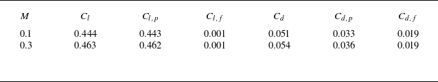
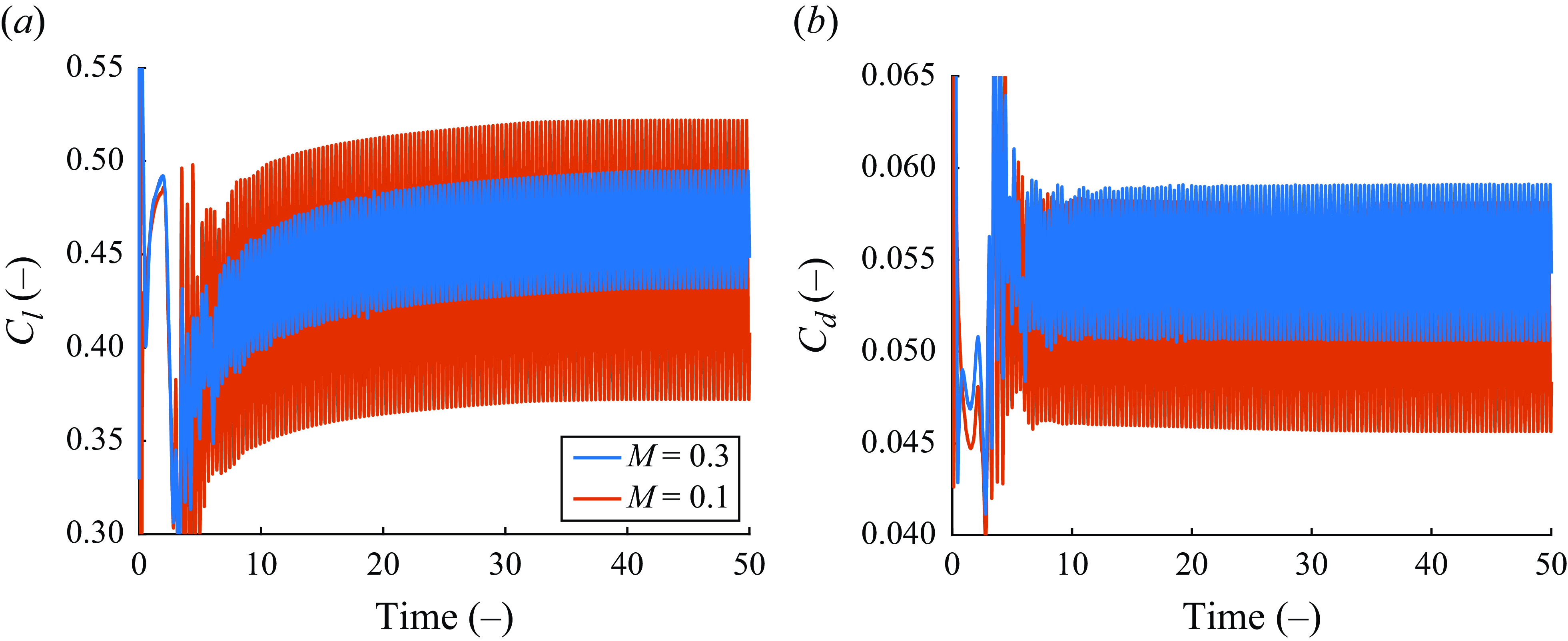
Figure 23. Lift and drag coefficients at
 $\alpha$
= 4
$\alpha$
= 4
 $^{\circ }$
over time for different Mach numbers. Domain radius
$^{\circ }$
over time for different Mach numbers. Domain radius
 $R$
= 30
$R$
= 30
 $c$
.
$c$
.
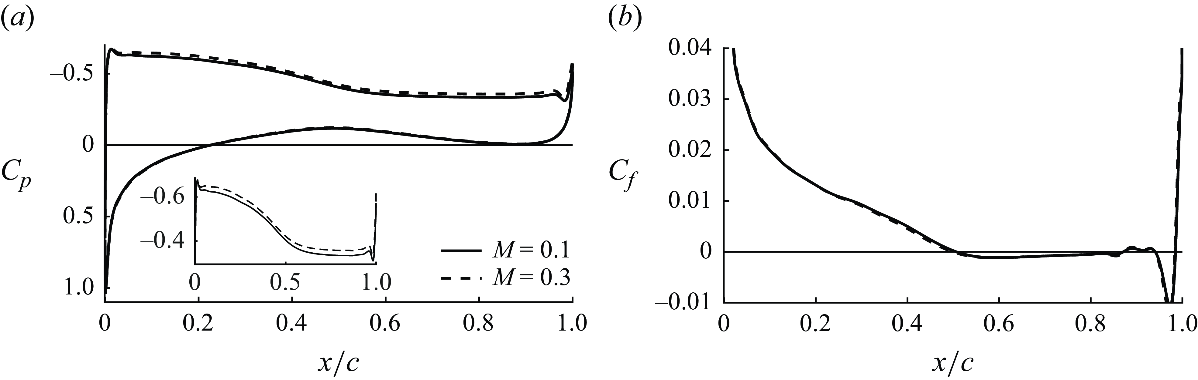
Figure 24. Time-averaged pressure and skin-friction coefficients for
 $M$
= 0.1 and
$M$
= 0.1 and
 $M$
= 0.3 at
$M$
= 0.3 at
 $\alpha$
= 4
$\alpha$
= 4
 $^{\circ }$
,
$^{\circ }$
,
 $R$
= 30
$R$
= 30
 $c$
.
$c$
.
At 8
 $^{\circ }$
incidence, a slender LSB stretches from the leading edge until
$^{\circ }$
incidence, a slender LSB stretches from the leading edge until
 $x_{r,8^{\circ }}/c$
= 0.45, 0.41 and 0.49 for
$x_{r,8^{\circ }}/c$
= 0.45, 0.41 and 0.49 for
 $M$
= 0.05, 0.1 and 0.3 respectively. The profiles of the pressure and skin-friction coefficients are given in figure 25 and show that the higher compressibility in case of
$M$
= 0.05, 0.1 and 0.3 respectively. The profiles of the pressure and skin-friction coefficients are given in figure 25 and show that the higher compressibility in case of
 $M$
= 0.3 results in a more distinct pressure plateau and elongated separation bubble with downstream reattachment compared to the lower-Mach-number cases. Streamlines of the time-averaged recirculating flow within the LSB are plotted in figure 27 and illustrate the difference in bubble sizes. The lift and drag coefficient averages differ by 2 % and 12 % respectively (see table 4) and can be attributed to the modified pressure distribution caused by the different LSB sizes.
$M$
= 0.3 results in a more distinct pressure plateau and elongated separation bubble with downstream reattachment compared to the lower-Mach-number cases. Streamlines of the time-averaged recirculating flow within the LSB are plotted in figure 27 and illustrate the difference in bubble sizes. The lift and drag coefficient averages differ by 2 % and 12 % respectively (see table 4) and can be attributed to the modified pressure distribution caused by the different LSB sizes.
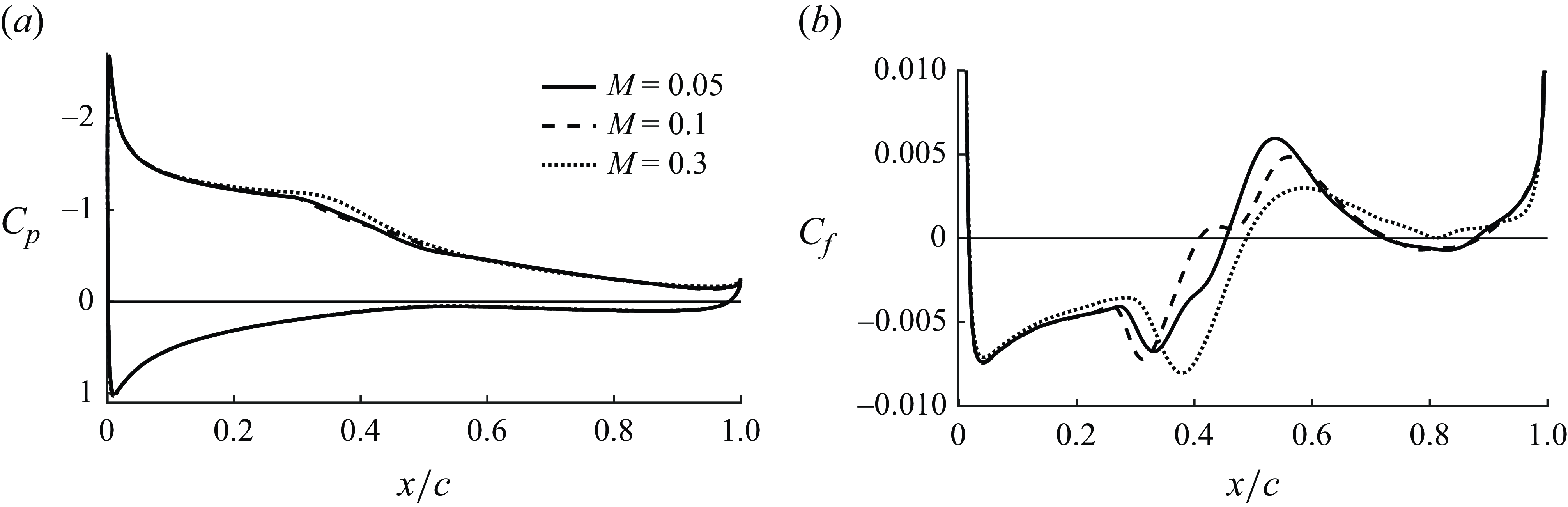
Figure 25. Time-averaged pressure and skin-friction coefficients for different Mach numbers at
 $\alpha$
= 8
$\alpha$
= 8
 $^{\circ }$
,
$^{\circ }$
,
 $R$
= 30
$R$
= 30
 $c$
.
$c$
.
Table 4. Lift and drag forces for
 $\alpha$
= 8
$\alpha$
= 8
 $^{\circ }$
and different Mach numbers.
$^{\circ }$
and different Mach numbers.
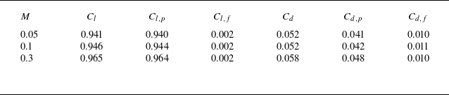
In addition to assessing compressibility effects by computing the flow at different Mach numbers with the compressible DGSEM solver, we also compare our results with incompressible flow simulations performed with FLUENT. Transient, incompressible computations are conducted with a pressure-based solver, second-order upwind for the spatial discretisation, and second-order implicit time stepping. No turbulence model is applied such that only source for artificial viscosity is through numerical dissipation from the upwinding scheme. A C-type domain with radius and wake length of 30 chords and consisting of 802 300 quadrilateral elements is used. The outer boundaries treated as velocity inflow (left, lower and upper) and pressure outflow conditions (right) and a no-slip condition is applied at airfoil surface.
Figure 26 shows the history of the lift and drag coefficients obtained from compressible DGSEM computations at a Mach number of
 $M$
= 0.05 and sixth-order polynomial representation and incompressible simulations with FLUENT. The results are in good agreement and confirm that the solution to this particular flow has converged across different numerical solvers. The case also shows that compressibility effects are not the cause for the disagreement with the USC wind tunnel experiments at
$M$
= 0.05 and sixth-order polynomial representation and incompressible simulations with FLUENT. The results are in good agreement and confirm that the solution to this particular flow has converged across different numerical solvers. The case also shows that compressibility effects are not the cause for the disagreement with the USC wind tunnel experiments at
 $\alpha$
= 8
$\alpha$
= 8
 $^{\circ }$
as all simulations show the transitioned state regardless of the Mach number.
$^{\circ }$
as all simulations show the transitioned state regardless of the Mach number.
A comparison of the streamlines inside the LSB (see figure 27) shows that the bubble size in the FLUENT computations is nearly identical with the DGSEM results at
 $M$
= 0.3, but deviates from the topology found at
$M$
= 0.3, but deviates from the topology found at
 $M$
= 0.05. While the differences between the DGSEM results are related to the compressibility effects, results from the FLUENT simulation are also affected by the lower order accuracy of the spatial and temporal discretisation and the increased numerical dissipation of the upwind scheme.
$M$
= 0.05. While the differences between the DGSEM results are related to the compressibility effects, results from the FLUENT simulation are also affected by the lower order accuracy of the spatial and temporal discretisation and the increased numerical dissipation of the upwind scheme.
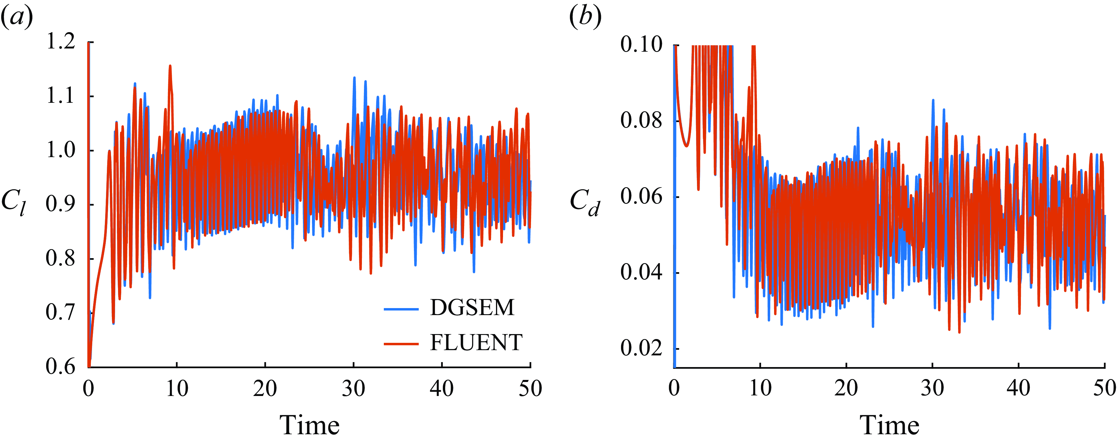
Figure 26. Lift and drag coefficients at
 $\alpha$
= 8
$\alpha$
= 8
 $^{\circ }$
over time DGSEM (
$^{\circ }$
over time DGSEM (
 $M$
= 0.05) and FLUENT (incompressible) computations.
$M$
= 0.05) and FLUENT (incompressible) computations.
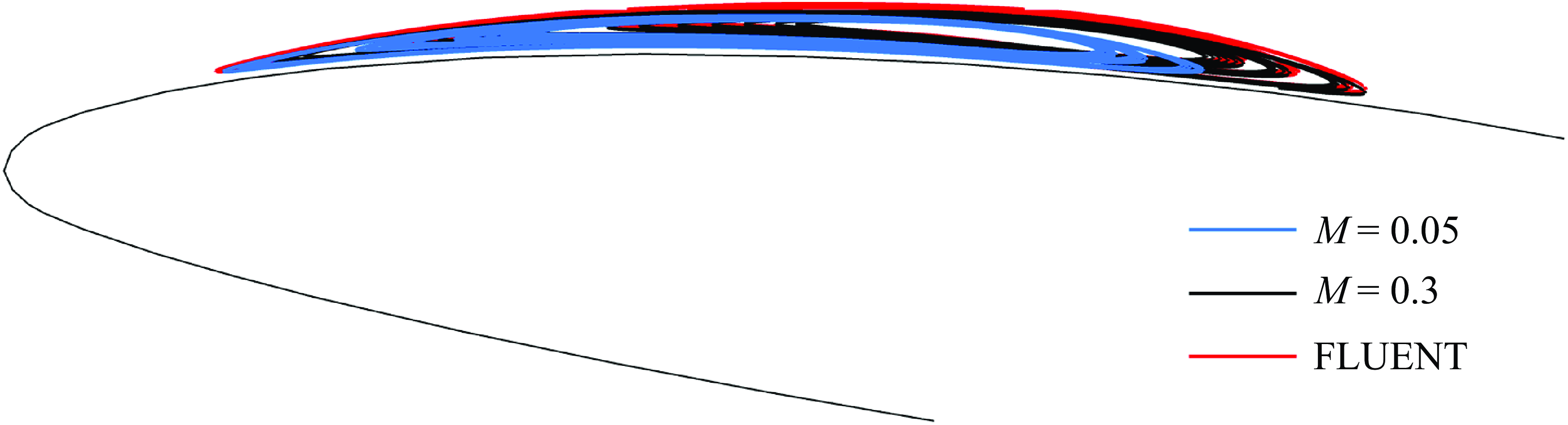
Figure 27. Laminar separation bubble for
 $M$
= 0.05 and
$M$
= 0.05 and
 $M$
= 0.3 (DGSEM) and incompressible (FLUENT) at
$M$
= 0.3 (DGSEM) and incompressible (FLUENT) at
 $\alpha$
= 8
$\alpha$
= 8
 $^{\circ }$
,
$^{\circ }$
,
 $R$
= 30
$R$
= 30
 $c$
.
$c$
.
A.2. Domain size
We assess the effect of domain size, blockage and spurious boundary reflections on the solution by comparing the aerodynamic forces, pressure and skin-friction coefficients for different sizes of the computational domain for several angles of attack.
Figure 28 illustrates the lift and drag coefficient for the flow at 4
 $^{\circ }$
incidence and domain radii from
$^{\circ }$
incidence and domain radii from
 $R$
= 3.5
$R$
= 3.5
 $c$
to
$c$
to
 $R$
= 50
$R$
= 50
 $c$
. Corresponding pressure and skin-friction distributions over the wing are plotted in figure 29 for
$c$
. Corresponding pressure and skin-friction distributions over the wing are plotted in figure 29 for
 $R$
= 3.5
$R$
= 3.5
 $c$
and 30
$c$
and 30
 $c$
. The free-stream boundaries show a strong impact on the pressure coefficient at the leading edge, which is significantly lower for the larger domain and indicates that the proximity of the boundaries for
$c$
. The free-stream boundaries show a strong impact on the pressure coefficient at the leading edge, which is significantly lower for the larger domain and indicates that the proximity of the boundaries for
 $R$
= 3.5
$R$
= 3.5
 $c$
forces the flow in this region. The pressure deviation is reflected in the trend of the lifting force with deviations of the time-averaged solution of 6 % between small and large domains (see table 5). As the discrepancies are mainly caused by the differences in the pressure distribution, the drag force shows only minor variations between the cases and converges more quickly. The strongly sinusoidal time dependency of the forces is maintained for all domain radii.
$c$
forces the flow in this region. The pressure deviation is reflected in the trend of the lifting force with deviations of the time-averaged solution of 6 % between small and large domains (see table 5). As the discrepancies are mainly caused by the differences in the pressure distribution, the drag force shows only minor variations between the cases and converges more quickly. The strongly sinusoidal time dependency of the forces is maintained for all domain radii.
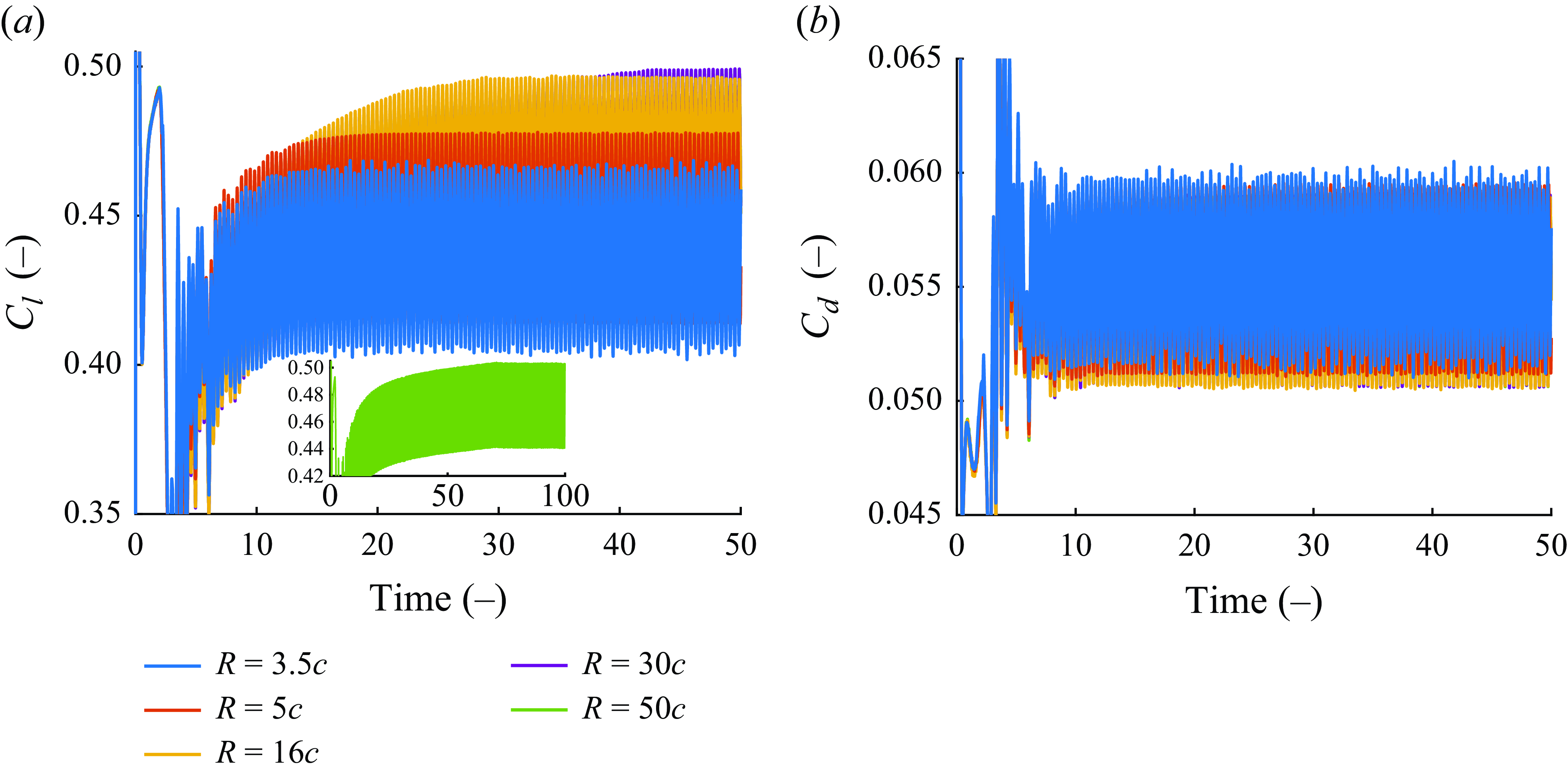
Figure 28. Lift and drag coefficients over time for different computational domain sizes and
 $\alpha$
= 4
$\alpha$
= 4
 $^{\circ }$
,
$^{\circ }$
,
 $M$
= 0.3.
$M$
= 0.3.
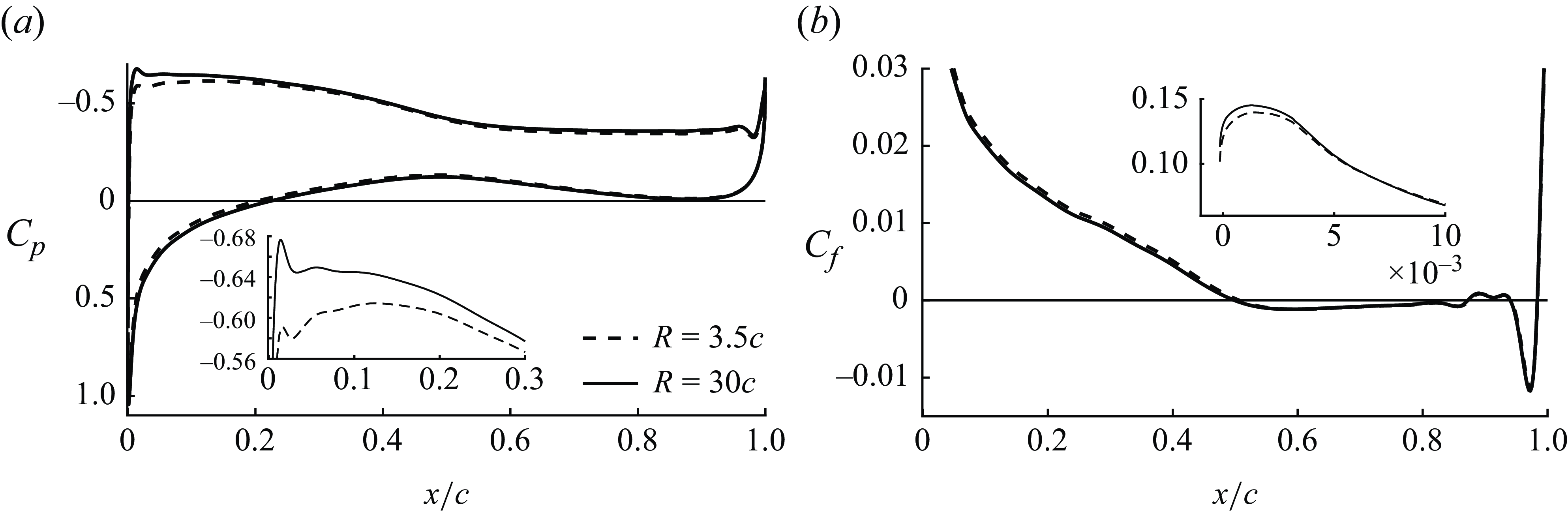
Figure 29. Time-averaged pressure and skin-friction coefficients for
 $R$
= 3.5
$R$
= 3.5
 $c$
and
$c$
and
 $R$
= 30
$R$
= 30
 $c$
at
$c$
at
 $\alpha$
= 4
$\alpha$
= 4
 $^{\circ }$
,
$^{\circ }$
,
 $M$
= 0.3.
$M$
= 0.3.
Table 5. Lift and drag coefficients for
 $\alpha$
= 4
$\alpha$
= 4
 $^{\circ }$
and different domain sizes.
$^{\circ }$
and different domain sizes.
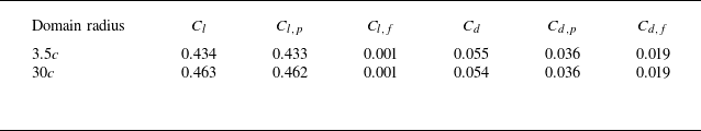
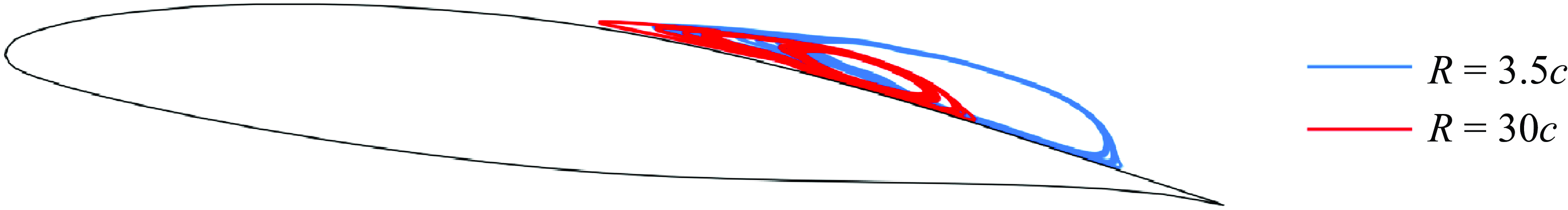
Figure 30. Laminar separation bubble for domain radii
 $R$
= 3.5
$R$
= 3.5
 $c$
and
$c$
and
 $R$
= 30
$R$
= 30
 $c$
at
$c$
at
 $\alpha$
= 7
$\alpha$
= 7
 $^{\circ }$
,
$^{\circ }$
,
 $M$
= 0.3.
$M$
= 0.3.
Because the magnitude of the pressure and friction forces increases with the flow angle, the influence of the free-stream boundaries also becomes more distinct. For 7
 $^{\circ }$
incidence, the separated boundary layer reattaches at the rear of the airfoil and forms a local LSB. Streamlines of the time-averaged solution within the separation bubble are plotted in figure 30 for domain sizes of
$^{\circ }$
incidence, the separated boundary layer reattaches at the rear of the airfoil and forms a local LSB. Streamlines of the time-averaged solution within the separation bubble are plotted in figure 30 for domain sizes of
 $R$
= 3.5
$R$
= 3.5
 $c$
and
$c$
and
 $R$
= 30
$R$
= 30
 $c$
. The LSB is significantly larger in the smaller domain where the free-stream boundaries impact the solution stronger by forcing the flow. The difference in LSB sizes is distinctly visible in the time-averaged profiles of the surface pressure and skin-friction coefficients, where both,
$c$
. The LSB is significantly larger in the smaller domain where the free-stream boundaries impact the solution stronger by forcing the flow. The difference in LSB sizes is distinctly visible in the time-averaged profiles of the surface pressure and skin-friction coefficients, where both,
 $C_p$
and
$C_p$
and
 $C_f$
, show the shift of the reattachment point of the LSB (see figure 31). Despite these significant differences in the flow topology, the time-averaged lift coefficient deviates only by 1.5 %, while the drag force differs by more than 40 % (see table 6). Note that the magnitude of the drag is only approximately 5 % of the lift force and hence is more susceptible to such changes.
$C_f$
, show the shift of the reattachment point of the LSB (see figure 31). Despite these significant differences in the flow topology, the time-averaged lift coefficient deviates only by 1.5 %, while the drag force differs by more than 40 % (see table 6). Note that the magnitude of the drag is only approximately 5 % of the lift force and hence is more susceptible to such changes.
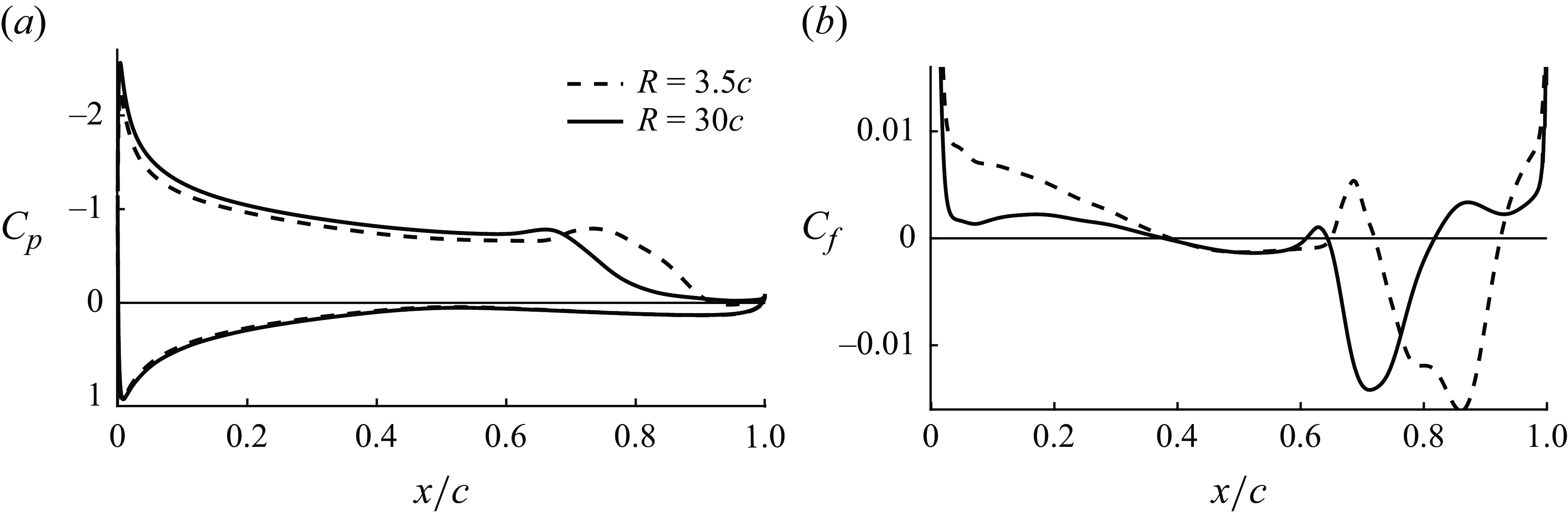
Figure 31. Time-averaged pressure and skin-friction coefficients for
 $R$
= 3.5
$R$
= 3.5
 $c$
and
$c$
and
 $R$
= 30
$R$
= 30
 $c$
at
$c$
at
 $\alpha$
= 7
$\alpha$
= 7
 $^{\circ }$
,
$^{\circ }$
,
 $M$
= 0.3.
$M$
= 0.3.
Table 6. Lift and drag coefficients for
 $\alpha$
= 7
$\alpha$
= 7
 $^{\circ }$
and different domain sizes.
$^{\circ }$
and different domain sizes.
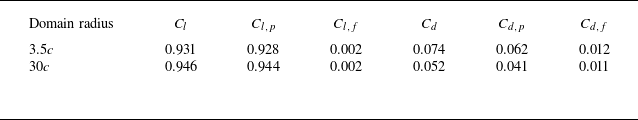
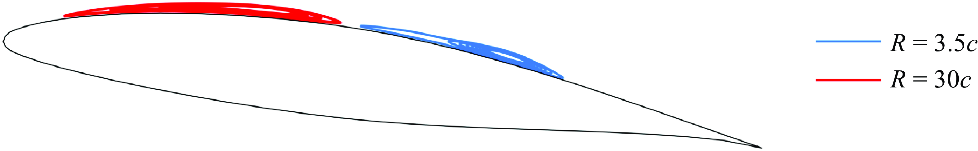
Figure 32. Laminar separation bubble for domain radii
 $R$
= 3.5
$R$
= 3.5
 $c$
and
$c$
and
 $R$
= 30
$R$
= 30
 $c$
at
$c$
at
 $\alpha$
= 8
$\alpha$
= 8
 $^{\circ }$
,
$^{\circ }$
,
 $M$
= 0.3.
$M$
= 0.3.
The effect of free-stream boundaries on the flow topology is even more pronounced at 8
 $^{\circ }$
incidence, where the location of the LSB completely shifts between the front and the rear side of the airfoil (see figure 32). This, again, is reflected in the surface pressure and the skin-friction coefficient (see figure 33), but curiously does not translate into a significant change in the integrated lift or the drag force, as summarised in table 7. The reason is that the bubble height is small and hence only slightly changes the pressure distribution, which remains approximately constant throughout separated flow regions. Given that both lift and drag coefficients are dominated by the pressure force (see table 7), the location of the LSB has only a limited affect on the lift as long as the bubble remains slender.
$^{\circ }$
incidence, where the location of the LSB completely shifts between the front and the rear side of the airfoil (see figure 32). This, again, is reflected in the surface pressure and the skin-friction coefficient (see figure 33), but curiously does not translate into a significant change in the integrated lift or the drag force, as summarised in table 7. The reason is that the bubble height is small and hence only slightly changes the pressure distribution, which remains approximately constant throughout separated flow regions. Given that both lift and drag coefficients are dominated by the pressure force (see table 7), the location of the LSB has only a limited affect on the lift as long as the bubble remains slender.
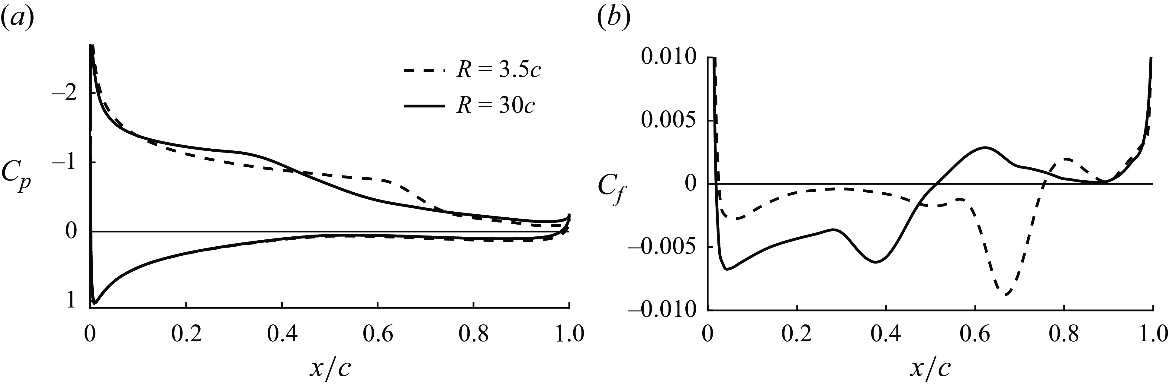
Figure 33. Time-averaged pressure and skin-friction coefficients for
 $R$
= 3.5
$R$
= 3.5
 $c$
and
$c$
and
 $R$
= 30
$R$
= 30
 $c$
at
$c$
at
 $\alpha$
= 8
$\alpha$
= 8
 $^{\circ }$
,
$^{\circ }$
,
 $M$
= 0.3.
$M$
= 0.3.
The parametric study of 2-D Navier–Stokes simulations show that, although the LSB location can be notably affected by changes in domain size, resolution and Mach number, the results do not indicate that any of the tested parameters move the critical angle of attack to higher values. Particularly, the good agreement between DGSEM and FLUENT simulations confirm that the flow at 8
 $^{\circ }$
incidence has converged to a reasonable level across different numerical solvers.
$^{\circ }$
incidence has converged to a reasonable level across different numerical solvers.
Table 7. Lift and drag coefficients for
 $\alpha$
= 8
$\alpha$
= 8
 $^{\circ }$
and different domain sizes.
$^{\circ }$
and different domain sizes.
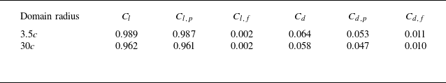
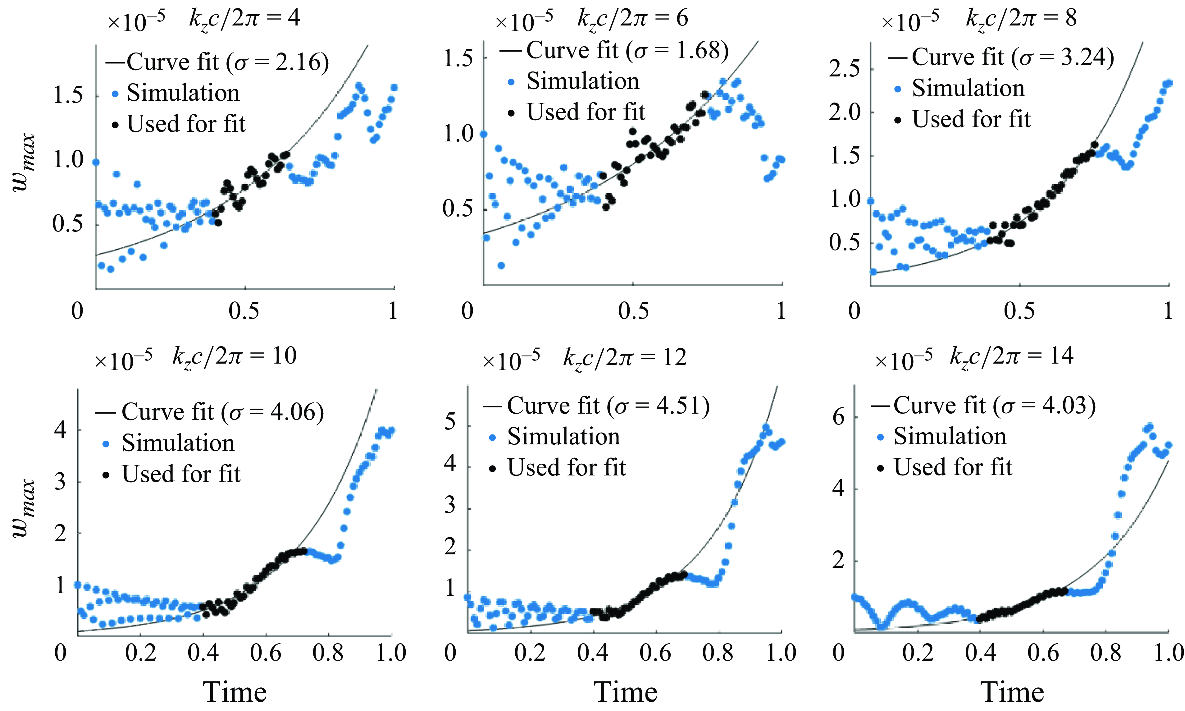
Figure 34. Growth of the perturbation velocity
 $w$
over time for different perturbation wavenumbers at
$w$
over time for different perturbation wavenumbers at
 $\alpha$
= 4
$\alpha$
= 4
 $^{\circ }$
.
$^{\circ }$
.
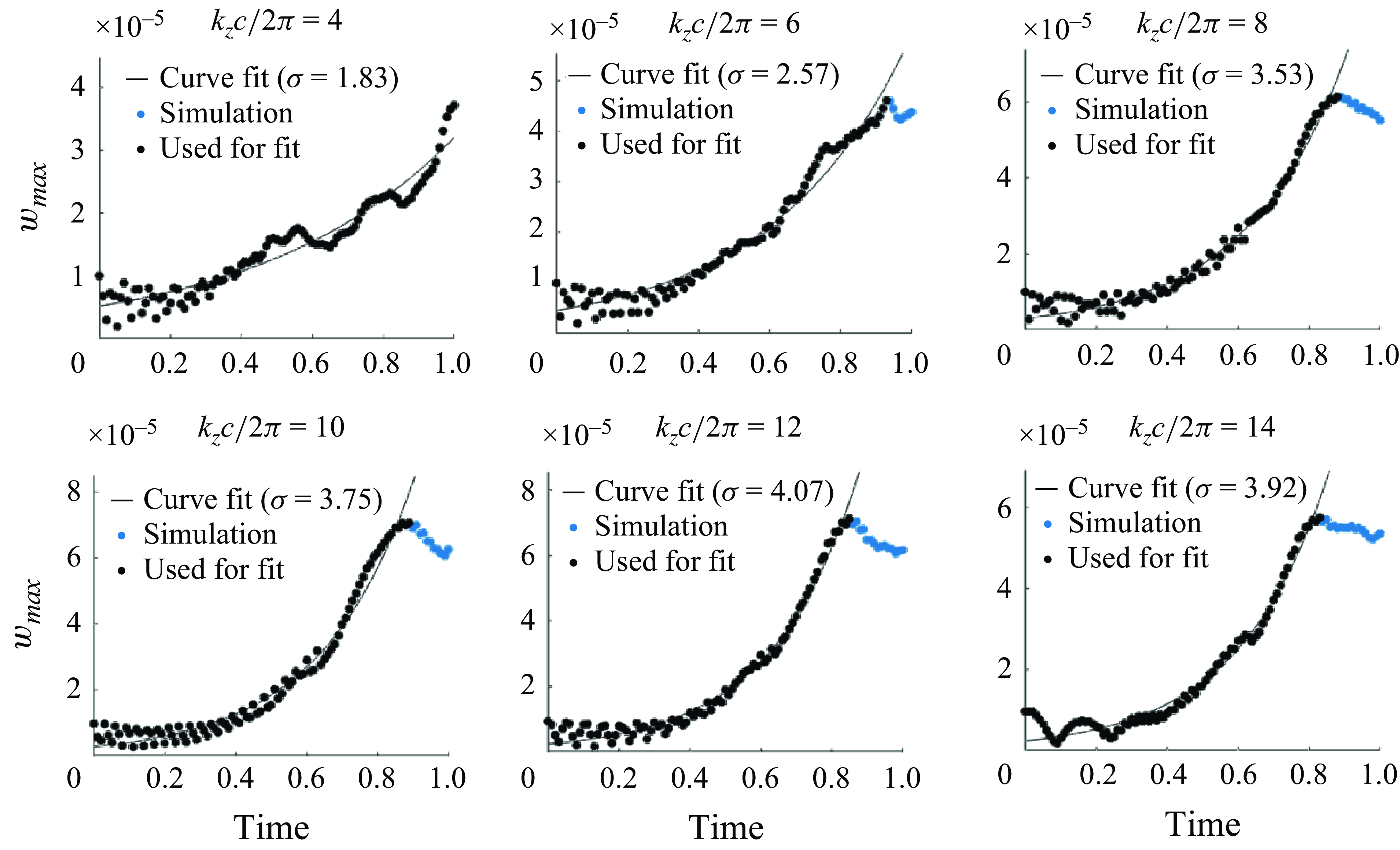
Figure 35. Growth of the perturbation velocity
 $w$
over time for different perturbation wavenumbers at
$w$
over time for different perturbation wavenumbers at
 $\alpha$
= 6
$\alpha$
= 6
 $^{\circ }$
.
$^{\circ }$
.
Appendix B. Extraction of perturbation growth rate
We extracted the growth of an initial perturbation within the near wake by perturbing a 2-D initial condition with a perturbation of the form
 \begin{equation} w = 10^{-5} \sin (2 \pi k_z z / c) \cdot e^{-((x / c - 1.0)^2 + (y / c - 0.05)^2) / 0.025}. \end{equation}
The maxima of the perturbation velocity
 $w$
are then tracked over time within the near wake (1
$w$
are then tracked over time within the near wake (1
 $\leqslant$
 $x/c$
$x/c$
 $\leqslant$
1.4) and fitted to a function
$\leqslant$
1.4) and fitted to a function
 $C_0 e^{\sigma t}$
via nonlinear regression. The results are given in figure 34 for
$C_0 e^{\sigma t}$
via nonlinear regression. The results are given in figure 34 for
 $\alpha$
= 4
$\alpha$
= 4
 $^{\circ }$
and figure 35 for
$^{\circ }$
and figure 35 for
 $\alpha$
= 6
$\alpha$
= 6
 $^{\circ }$
. The black dots indicate which data points contribute to the exponential growth fit.
$^{\circ }$
. The black dots indicate which data points contribute to the exponential growth fit.


 Open access