


Crossref Citations
This article has been cited by the following publications. This list is generated based on data provided by Crossref.
Shi, Yanxiong
Liu, Hongyou
and
Zheng, Xiaojing
2025.
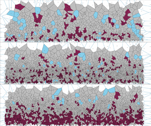
Evolution of two-phase structures during the entire sandstorm process.
Journal of Fluid Mechanics,
Vol. 1007,
Issue. ,