


1. Introduction
Convection in porous media is an important process in numerous geological settings, ranging from geothermal heat transport to subsurface salt fingering (Nield & Bejan Reference Nield and Bejan2017). Over the last ten years, study in this area has intensified, driven in part by the importance of convection as a mechanism for aiding secure geological sequestration of carbon dioxide (Huppert & Neufeld Reference Huppert and Neufeld2014).
In many of these settings, convection is driven by a dense or buoyant source distributed along one boundary. In the context of CO $_2$ sequestration, for example, the distributed source represents an injected pool of buoyant CO
 $_2$ within an aquifer. CO
 $_2$ is weakly soluble in water, but the resultant solution that forms at the interface is more dense than water; it can thus be unstable to downwelling convection, leading to enhanced dissolution and longer term security of CO
 $_2$ storage. Numerous authors have used numerical and theoretical techniques to investigate different aspects of the ‘lifecycle’ of convection driven in this way, from initial diffusive growth and convective instability of a growing dense (or buoyant) layer (e.g. Riaz, Hesse & Tchelepi Reference Riaz, Hesse, Tchelepi and Orr2006; Rapaka et al. Reference Rapaka, Pawar, Stauffer, Zhang and Chen2009; Slim & Ramakrishnan Reference Slim and Ramakrishnan2010; Daniel, Riaz & Tchelepi Reference Daniel, Riaz and Tchelepi2015; Tilton Reference Tilton2018), to the development of large-scale convective fingering patterns and stabilisation of the convective flux (e.g. Fu, Cueto-Felgueroso & Juanes Reference Fu, Cueto-Felgueroso and Juanes2013; Slim Reference Slim2014) to the gradual decay and ‘shutdown’ of convection as the ambient fluid becomes saturated (Hewitt, Neufeld & Lister Reference Hewitt, Neufeld and Lister2013; Slim Reference Slim2014). This behaviour has also been investigated using analogue laboratory experiments (e.g. Backhaus, Turitsyn & Ecke Reference Backhaus, Turitsyn and Ecke2011; Slim et al. Reference Slim, Bandi, Miller and Mahadevan2013; De Paoli, Alipour & Soldati Reference De Paoli, Alipour and Soldati2020).
There have been many extensions to this canonical problem to investigate the role of additional physical effects on convection (see e.g. Hewitt (Reference Hewitt2020) for a review of these). In particular, most naturally occurring media are, to some degree, heterogeneous and anisotropic, and a number of studies have explored the effect of heterogeneity or anisotropy on evolving convection from a distributed source (Elenius & Gasda Reference Elenius and Gasda2013; De Paoli, Zonta & Soldati Reference De Paoli, Zonta and Soldati2017; Green & Ennis-King Reference Green and Ennis-King2018; Soboleva Reference Soboleva2018). While heterogeneity and anisotropy can, in general, be rather variable, certain canonical forms of heterogeneity occur frequently in natural media; one such form is layering. Here, we are particularly concerned with thin, low-permeability baffles or layers that intersperse a host medium with a roughly regular vertical spacing, which are a relatively common feature of geological sedimentary formations (Phillips Reference Phillips2009). The aim of this work is to understand the impact that an idealised series of thin, horizontal, low-permeability layers have on strong convective flow driven by a dense, distributed source along an upper boundary. For this task, we use numerical simulations to motivate the development of simple theoretical models that describe the evolution of the mean density field and convective fluxes.
The impact of one such thin layer was the subject of a previous numerical study by Soboleva (Reference Soboleva2018), who demonstrated various qualitative features of how the layer affected convective flow across it. This study did not, however, go on to explore the problem theoretically or give any quantitative scalings to delineate different behaviour. In related experimental work, Salibindla et al. (Reference Salibindla, Subedi, Shen, Masuk and Ni2018) used a horizontal line of posts placed across a Hele-Shaw cell to create a thin region of higher resistance to flow. They found, however, that the effective permeability of this region did not provide the dominant control on the flow in their experiments; that is, it did not constitute a macroscopic low-permeability layer. Instead, the local geometry of the posts and the gaps between them, which were of a comparable scale to the downwelling convective fingers, controlled the flow across the region.
More generally, the impact of layered heterogeneity on convection has been explored in different settings. The behaviour of isolated plumes in layered media has been the subject of experimental and theoretical work in the context of a step jump in the permeability (Sahu & Flynn Reference Sahu and Flynn2017; Bharath, Sahu & Flynn Reference Bharath, Sahu and Flynn2020) and numerical and theoretical work in the case of an isolated plume crossing a single thin, low-permeability layer (Hewitt, Peng & Lister Reference Hewitt, Peng and Lister2020). Statistically steady convection, driven by a dense source along an upper boundary and a buoyant source along a lower boundary, has also been explored in the presence of a thin layer, for weak (McKibbin & Tyvand Reference McKibbin and Tyvand1983) and strong (Hewitt, Neufeld & Lister Reference Hewitt, Neufeld and Lister2014) convective flow. This last study showed that, provided the low-permeability layer is sufficiently thin relative to the host medium, and the permeability is sufficiently low, its resistance to flow can be parameterised by an impedance parameter,  $\varOmega$, which provides a dimensionless ratio of the layer's thickness to its permeability. This parameterisation, which avoids the need to resolve the dynamics within each thin low-permeability layer directly, was also employed by Hewitt et al. (Reference Hewitt, Peng and Lister2020), and we use it again in the present study, as outlined in § 2.
The paper is laid out as follows. The set-up, governing equations, scalings and modelling assumptions are outlined in § 2. Some numerical observations of the system are presented in § 3, in order to frame the subsequent theory. This is described in § 4, with consideration given to different limits in which the thin layers play either a negligible or a dominant role on the evolution of the convective flow. The findings and implications of this work are briefly summarised in § 5.
2. Model
2.1. Model set-up
Consider a dense, distributed source of solute located along the impermeable upper boundary of a two-dimensional porous medium that is initially saturated with a fluid of a uniform density. The impermeable lower boundary of the medium lies a distance  $L^{*}$ below the upper surface. The medium is isotropic and has uniform permeability
  $K^{*}$, except in a series of
  $n$ thin, horizontal layers which divide the medium into
  $n+1$ regions of equal depth (see figure 1). The layers have permeability
  $\epsilon _K K^{*}$, for some
  $\epsilon _K \ll 1$. The vertical distance between the centre of any two layers is
  $H^{*}$, such that the depth of the medium is
  $L^{*} = (n+1) H^{*}$, while the thin layers themselves have a thickness
  $\epsilon _H H^{*}$, with
  $\epsilon _H \ll 1$. The whole medium is taken to have uniform porosity
  $\phi$; any effect of a lower porosity in the thin layers is presumed to be dominated by the associated reduction in the permeability, which is already accounted for. This approximation is briefly discussed in § 5.

Figure 1. A schematic of the model set-up in terms of (a) dimensional and (b) non-dimensional quantities. The permeability in the low-permeability layers is a factor  $\epsilon _K \ll 1$ smaller than that in the host medium. In the dimensionless formulation, rather than resolving the dynamics within each thin layer, they are parameterised by the layer's impedance
  $\varOmega = \epsilon _H/\epsilon _K$ according to the jump condition in (2.15).
We take a coordinate system  $(x,z)$ with origin located on the upper boundary. We consider a situation in which the concentration
  $c^{*}$ of a solute controls the density
  $\rho$ of fluid according to a linear equation of state
 \begin{equation} \rho = \rho_0\left( 1 + \alpha c^{*}\right), \end{equation}
with  $\alpha >0$ and reference density
  $\rho _0$. The upper boundary is held at a fixed concentration
  $c_0 >0$, while the saturating fluid in the medium initially has zero concentration. Under the Boussinesq approximation, the flow
  $\boldsymbol {u}^{*} = (u^{*},w^{*})$ in the medium is incompressible and obeys Darcy's law, while the concentration evolves over time
  $t^{*}$ by advection and diffusion, as described by
 \begin{gather} \boldsymbol{\nabla} \boldsymbol{\cdot} \boldsymbol{u}^{*} = 0, \end{gather}
 \begin{gather}\boldsymbol{u}^{*} ={-}\frac{k^{*}}{\mu} \left(\boldsymbol{\nabla} p^{*} + \rho g \hat{\boldsymbol{z}} \right), \end{gather}
 \begin{gather}\phi \frac{\partial {c^{*}}}{\partial {t^{*}}} + u^{*} \frac{\partial {c^{*}}}{\partial {x^{*}}} + w^{*} \frac{\partial {c^{*}}}{\partial {z^{*}}} = \phi D \nabla^{2} c^{*}, \end{gather}
where  $\hat {\boldsymbol {z}}$ is a unit vector in the vertical direction,
  $p^{*}$ is the pore pressure,
  $g$ is the gravitational acceleration and
  $\mu$ and
  $D$ are the viscosity and effective diffusivity, respectively, both of which are assumed to be constant. The permeability
  $k^{*}$ is equal to
  $K^{*}$ outside the
  $n$ low-permeability layers and to
  $\epsilon _K K^{*}$ inside the layers. Note that the assumption of a constant diffusivity parameter, as opposed to a flow-dependent dispersivity, is valid as long as the flow is sufficiently slow that the pore-scale Péclet number remains small (Woods Reference Woods2015); this is expected to be a reasonable assumption in many geological settings involving convection (Hewitt Reference Hewitt2020), although it can be a harder limit to attain in analogue laboratory experiments.
2.2. Non-dimensional equations
We define the following scales for the buoyancy velocity and the length and time scales over which advection and diffusion balance:
 \begin{equation} u_0 = \frac{\rho_0 \alpha c_0 g K^{*}}{\mu},\quad z_0 = \frac{\phi D}{u_0},\quad t_0 = \frac{\phi z_0}{u_0} = \frac{\phi^{2} D}{u_0^{2}}, \end{equation}
and further introduce dimensionless (unstarred) variables via
 \begin{gather} \boldsymbol{u} = \frac{ \boldsymbol{u}^{*}}{u_0},\quad (x,y,z) = \frac{(x^{*},y^{*},z^{*})}{z_0},\quad c = \frac{c^{*}}{c_0},\quad k = \frac{k^{*}}{K^{*}}, \end{gather}
 \begin{gather}t = \frac{t^{*}}{t_0},\quad p = \frac{K^{*}}{\phi D \mu } \left(p^{*} + \rho_0 g z^{*}\right), \end{gather}
where, in the final expression, we have scaled out the background hydrostatic pressure gradient associated with the reference density  $\rho _0$. Given these scalings, the governing equations (2.2)–(2.4) reduce to
 \begin{gather} \boldsymbol{\nabla}\boldsymbol{\cdot}\boldsymbol{u} = 0,\quad \boldsymbol{u} ={-}k\left(\boldsymbol{\nabla} p + c \hat{\boldsymbol{z}} \right), \end{gather}
 \begin{gather}\frac{\partial {c}}{\partial {t}} + \boldsymbol{u}\boldsymbol{\cdot}\boldsymbol{\nabla} c = \nabla^{2} c, \end{gather}
where the dimensionless permeability is
 \begin{equation} k = \left\{\begin{array}{@{}cc} \epsilon_K & \left\{({-}j-\epsilon_H/2) < z/H < ({-}j + \epsilon_H/2),\ j =1,2,\ldots n\right\}, \\ 1 & \text{otherwise}. \end{array}\right. \end{equation}
With this choice of scaling, the dimensionless distance  $H$ between the centre of each layer,
 \begin{equation} H = \frac{u_0 H^{*}}{\phi D} = \frac{ \rho_0 \alpha c_0 g K^{*} H^{*}}{\phi D \mu}, \end{equation}
takes the form of a Rayleigh number for the system, and the domain has depth
 \begin{equation} L = (n+1) H. \end{equation}
The focus of this work is on the limit in which convection provides a much more efficient transport mechanism than diffusion; that is, when  $H \gg 1$.
The impermeable upper boundary is held at a fixed concentration, so  $w(z=0) = 0$ and
  $c(z=0) = 1$. There is no transport of solute through the base of the domain,
  $\partial c/\partial z = w = 0$ on
  $z=-L$, and the domain is initially filled with unsaturated fluid,
  $c(t=0) = 0$. We assume periodic boundaries in the
  $x$ direction, with a domain width
  $X \gg H$.
2.3. The impedance
In this study, rather than resolving the dynamics in each thin, low-permeability layer, we parameterise the layer by its impedance
 \begin{equation} \varOmega = \frac{\epsilon_H}{\epsilon_K}. \end{equation}
The impedance provides a ratio of the scaled thickness  $\epsilon _H$ to the scaled permeability
  $\epsilon _K$ of the low-permeability layers, both relative to the equivalent values in the regions between the layers. The role of
  $\varOmega$ becomes clear by considering the vertical component of Darcy's law (2.8b) in the
  $j$th low-permeability layer
 \begin{equation} w ={-}\epsilon_K \left(\frac{\partial {p}}{\partial {z}} + c \right) ={-}\epsilon_K \left[\frac{ [p]_j }{\epsilon_H H} + O((\epsilon_H H)^{2}) + c \right]\approx{-}\frac{\epsilon_K [p]_j }{\epsilon_H H}, \end{equation}
provided  $\epsilon _K, \epsilon _H \ll 1$. Here,
  $[p]_j$ signifies the pressure jump across the
  $j$th layer, and the approximation of the pressure gradient follows from a Taylor expansion of the pressure centred on the middle of that layer. We can thus parameterise the effect of each layer by applying the jump condition
 \begin{equation} \varOmega H \left. w\right|_{z={-}jH} ={-}[p]_j, \end{equation}
or, more usefully, its horizontal derivative
 \begin{equation} \varOmega H \left. \frac{\partial {w}}{\partial {x}}\right|_{z={-}jH} = [u]_j, \end{equation}
at  $z = -jH$, for
  $j=1,\ldots n$. If
  $\varOmega$ is small, then the pressure difference across the low-permeability layers will be small, and so they should have a negligible impact on the flow. On the other hand, if
  $\varOmega$ is large then substantial pressure differences will be required to drive flow across the layers, which will either result in very significant adjustments to the flow or will mean that no flow can be driven across the layers at all.
Previous studies of both statistically steady and evolving convection (Hewitt et al. Reference Hewitt, Neufeld and Lister2014, Reference Hewitt, Peng and Lister2020) have demonstrated by comparison with fully resolved simulations that this reduction is accurate provided  $\epsilon _K \ll 1$ and
  $\epsilon _H \ll 1$. As such, we work with this parameterised form of the layers throughout this study (see figure 1). Note that underlying this reduction – and indeed underlying the use of Darcy's law throughout the domain – is the assumption that the pore scale everywhere remains small compared with any other length scale in the problem. This was not the case, for example, in the experiments of Salibindla et al. (Reference Salibindla, Subedi, Shen, Masuk and Ni2018) outlined in the introduction, in which the flow through a high-resistance layer in a Hele-Shaw cell was controlled by the macroscopic gaps between posts in the cell, rather than by the computed effective impedance of that region.
Given this reduction, the problem is governed by the parameter-free set of (2.8a,b) and (2.9) (with  $k=1$ everywhere), together with the jump condition (2.16) applied at the centreline of each layer. The governing parameters are the dimensionless distance
  $H \gg 1$ between the layers, the number of layers
  $n$ and the impedance
  $\varOmega$ of the layers.
2.4. Numerical details
Equations (2.8a,b) and (2.9) were solved numerically using a combined spectral and finite-difference approach. Away from the low-permeability layers, (2.8a,b) can be reduced to a Poisson equation for the streamfunction  $\psi$, where
  $(u,w) = (\partial \psi /\partial z, -\partial \psi /\partial x)$ (see e.g. Hewitt Reference Hewitt2020). At each time step, this equation was solved by means of a horizontal Fourier transform coupled with standard second-order finite differences in the vertical direction, which results in a tridiagonal-matrix-inversion problem. Before solving, this problem was modified to account for the parameterised low-permeability layers: each of the
  $n$ rows of the tridiagonal matrix corresponding to the centreline of each layer was replaced by an equation that imposed the Fourier transform of the jump condition (2.16) instead of (2.8a,b). The velocity field everywhere followed from solving the resultant tridiagonal problem and inverting the Fourier transform. The transport equation (2.9) was solved on the whole domain using a standard second-order finite-difference discretisation, together with an alternating-direction implicit method with a predictor–corrector step for the nonlinear advection terms.
The spatial resolutions were chosen to ensure that the smallest convective scales were accurately captured. Recall that we have scaled lengths by the scale over which advection and diffusion balance, in (2.5a–c), and so we expect the smallest scales of the flow to be no less than  $O(1)$, compared with the scale of the domain (
 $O(H \gg 1$)). In fact, the smallest plumes that develop are found to have widths of around
  $100$, in these dimensionless units, and so a horizontal grid spacing of less than
  $20$ units was ensured in all simulations here. In the vertical, we expect narrow boundary-layer structures (that is, of an
  $O(1)$, rather than
  $O(H)$, extent) near the upper boundary and, for the right range of
  $\varOmega$, near the low-permeability layers. As such, a vertical stretching function was used to increase resolution near each layer and near the boundaries, in such a manner that ensured there were at least six grid points within any vertical boundary layer, without adding superfluous points between layers. In all simulations, the width of the domain was taken to be
  $X = 1.2 \times 10^{5}$ and
  $2^{13}$ grid points in the horizontal were used. Simulations were carried out at four different values of
  $H = [1.25,2.5,5,10] \times 10^{3}$, with
  $n$ ranging between one and eight; as such, the vertical extent of the domain was different in different simulations, but we typically used between
  $300$ and
  $500$ vertical grid points. Most simulations were repeated three times, with a very slightly different vertical resolution, to enable ensemble averaging of the results. A few verification simulations were carried out with substantially more vertical grid points to ensure the resolution in all vertical boundary layers was sufficient, and no statistically significant variations were observed.
As a result of taking a fixed width  $X$, the aspect ratio of the whole domain
  $X/L = X/(n+1)H$ varies with
  $n$ and
  $H$. The value of
  $X$ was chosen to be large relative to the predicted scales of convective motion in the absence of layers, so that any dependence on the specific choice of
  $X$ should be very small. As we will see, however, in the presence of layers the scale of the flow structures can, in some cases, grow substantially to fill the domain, and it is likely that there is some mode restriction at late times from our choice of
  $X$ in those cases, as discussed in § 4.3.3.
3. Results
In this section we outline how solutions vary with the impedance of the layer for a particular set of parameters ( $H=5000$,
  $n=8$), in order to frame the subsequent analysis.
3.1. Initial spreading
The dynamics of the system at very early times is not the primary focus of this study: provided  $H \gg 1$, the presence of the low-permeability layers will have negligible effect on the initial diffusive spread and convective instability in this system, because the layers are so far below the upper boundary. The ‘onset’ problem has received a great deal of attention in recent years (see e.g. Riaz et al. Reference Riaz, Hesse, Tchelepi and Orr2006; Rapaka et al. Reference Rapaka, Pawar, Stauffer, Zhang and Chen2009; Slim & Ramakrishnan Reference Slim and Ramakrishnan2010; Tilton Reference Tilton2018), and so here we simply describe the basic details. Note that, for much smaller
  $H$, the low-permeability layers may be sufficiently close to the upper boundary to influence the onset problem, and situations of this kind were considered by Daniel et al. (Reference Daniel, Riaz and Tchelepi2015).
Solute initially enters the domain by diffusion through the upper boundary. Over time, this growing boundary layer of dense solute becomes convectively unstable: small perturbations in the boundary layer are able to grow, driving the initiation of finger-like convective structures which advect solute away from the upper boundary much more efficiently that by diffusion alone. As they grow and merge, the flow takes the form of interleaving dense downwelling and buoyant upwelling plumes, and the associated convective flux through the upper boundary becomes statistically constant.
Figure 2 shows snapshots from simulations at three times soon after this stabilisation of the flux. The evolving structure of the flow in a homogeneous medium ( $\varOmega = 0$) can be seen in figure 2(a,d,g). Large downwelling fingers, which are fed by small ‘protoplumes’ located in a very thin boundary layer at the top of the domain, coarsen over time as they spread downwards, and the flow in the domain is predominantly vertical apart from in the narrow boundary-layer region. In the presence of layers, however, the dynamics is somewhat different. For a moderate impedance (figure 2b,e,h), it is clear that the low-permeability layer modulates the structure of the flow, causing descending plumes to spread laterally above each low-permeability layer, and ascending plumes to spread below each layer. Nevertheless, the essential structure of descending and ascending fingers of dense and buoyant fluid remains. For rather larger values of the impedance (figure 2c,f,i), the low-permeability layer can act as a complete barrier to flow and dense solute ‘pools’ above the first low-permeability layer. As diffusion carries solute over the low-permeability layer, small plumes begin to form below it, and over time these convective instabilities act to spread solute throughout the region above the next low-permeability layer. There does not appear to be any advective transport over the layer in this limit (no streamlines cross the layers in figure 2c,f,i).

Figure 2. Snapshots of the concentration and streamlines (black) from simulations with  $H=5\times 10^{3}$,
  $n=8$ and (a,d,g)
  $\varOmega = 0$, (b,e,h)
  $\varOmega = 0.2$ and (c,f,i)
  $\varOmega = 12.8$. Snapshots taken at times
  $t=16H$ (a–c),
  $32 H$ (d–f) and
  $64 H$ (g–i). For clarity, only a subset of the full domain – which can be seen in the subsequent two figures – is shown.
3.2. Subsequent and eventual spreading
Figures 3 and 4 show snapshots from simulations for different impedance  $\varOmega$ at later times. In the homogeneous medium (figure 3a,c), the descending plumes reach the impermeable base of the domain (figure 3a), where dense solute begins to spread laterally and gradually to fill up the domain. Once this dense fluid has backed up to the upper boundary, convection will begin to ‘shutdown’, as solute continues to be transported downwards, but through an increasingly dense ambient fluid (figure 3c). Eventually, the ambient concentration will have increased sufficiently that convection stops completely, because the driving density difference becomes too weak.

Figure 3. Snapshots of the concentration and streamlines (black) from simulations with  $H=5\times 10^{3}$,
  $n=8$ and (a,c)
  $\varOmega = 0$, (b,d)
  $\varOmega = 0.2$. Snapshots taken at times
  $t=64H$ (a,b) and
  $512 H$ (c,d).

Figure 4. Snapshots of the concentration and streamlines (black) from simulations with  $H=5\times 10^{3}$,
  $n=8$ and (a,c)
  $\varOmega = 0.8$, (b,d)
  $\varOmega = 12.8$. Snapshots taken at times
  $t=256H$ (a,b) and
  $1024 H$ (c,d).
For a relatively low impedance, the picture is qualitatively similar (figure 3b,d). Although the presence of the low-permeability layers modulates the structure of the interleaving plumes (figure 3b), the basic description of solute filling the domain and causing the convective flux to weaken as the ambient becomes saturated still holds. Note, however, that the low-permeability layers lead to a somewhat larger dominant horizontal length scale in this shutdown state.
For larger impedance (figure 4a,c), the low-permeability layers play a more significant role in the evolving dynamics. Plumes again spread down through the domain, but the presence of small protoplumes underneath internal low-permeability layers (figure 4a) indicates the presence of unstable diffusive boundary layers, revealing that diffusion across layers plays a role in solute transport as well as advection. Over time solute again saturates the entire domain, but the lateral scale of the plumes is much larger than for lower  $\varOmega$ (figure 4c). For even larger impedance (figure 4b), solute spreads by diffusion across layers, with convective mixing in the regions between each layer, for a long time. However, this arrangement can also eventually become unstable to the formation of a large-scale flow across all the layers, which is then able to spread solute throughout the domain (figure 4d). The lateral length scale of this flow is once again larger than at smaller values of
  $\varOmega$.
3.3. The flux
The flux of solute both into the domain across the upper boundary and across each of the low-permeability layers allows us to interpret some of the observations made above. The total flux  $F(t)$ into the domain is
 \begin{equation} F(t) = \frac{1}{X} \int_0^{X} \left.\frac{\partial {c}}{\partial {z}}\right|_{z=0} {{\rm d}}\kern0.06em {x}, \end{equation}
and we introduce the notation  $F_i$ for the flux across the
  $i$th low-permeability layer,
 \begin{equation} F_i(t) = \frac{1}{X} \int_0^{X} \left.\left(\frac{\partial {c}}{\partial {z}} - w c \right)\right|_{z={-}iH} {{\rm d}}\kern0.06em {x}. \end{equation}
 Figure 5(a) shows  $F(t)$ for various values of
  $\varOmega$. In all cases, once convection is established below the upper boundary (
 $t \sim 10^{4}$; Hewitt Reference Hewitt2020), the flux approaches a constant mean value
  $F \approx 0.017$, around which it exhibits chaotic fluctuations. In a homogeneous medium, this state persists while the convective plumes spread downwards and reach the base of the domain. Once the signal from the plumes reaching the impermeable base reaches the upper boundary, the flux begins to decrease as ambient fluid becomes saturated with solute. Previous studies have shown this to take a time of roughly
  $15 L = 15(n+1) H$. After this time, the flux begins to drop as the driving density difference decreases.

Figure 5. (a) The buoyancy flux  $F(t)$ through the upper boundary, ensemble averaged over three repeat simulations, for
  $H=5\times 10^{3}$,
  $n=8$ and
  $\varOmega = [0,0.05,0.2,0.8,3.2,12.8,51.2]$ (from blue to green to orange to dark red). The dashed horizontal line gives the statistically steady flux
  $F \approx 0.017$ in an unbounded domain. (b) The corresponding fraction of the flux that is advective through the first low-permeability layer at
  $z=-H$.
If the impedance of the layer is sufficiently large, however, the figure shows that the initial decrease in flux occurs somewhat earlier than this. This early decrease occurs because if the first low-permeability layer can act as a barrier to flow, sufficient solute can ‘back up’ and limit the supply of unsaturated fluid near the upper boundary, causing the flux to decrease. We expect this process to occur after a time of only  $\approx 15 H$ (as opposed to
  $15(n+1)H$). In fact, all the non-zero values of
  $\varOmega$ shown in figure 5(a) exhibit some decrease in the flux after this time. However, for low
  $\varOmega$, the flux fairly rapidly stops decaying and oscillates around a roughly constant or weakly increasing value, before eventually decaying again on roughly the same trajectory as the homogeneous medium. For larger values of
  $\varOmega$, the behaviour of
  $F(t)$ is similar, but with a longer initial decay and a more pronounced rise in
  $F$ once it stops decaying.
The initial decay of the flux for non-zero  $\varOmega$ can be explained by saturation of the ambient medium near the upper boundary, reducing the driving density difference there. figure 5(b) provides an interpretation for the subsequent deviation of the flux from that decaying trajectory. This figure shows the proportion of the total flux across the first low-permeability layer that comes from advection. The point where the flux leaves its decaying trajectory can be seen to coincide with a substantial increase in this proportion. That is, the flux begins to decay as the flow is unable to provide sufficient fresh fluid to maintain the driving density difference at the upper boundary, but there is a subsequent reorganisation of the flow that allows for increased advective transport across the layers, and is more efficiently able to supply fresh fluid to the upper part of the domain. This reorganisation is more pronounced at larger
  $\varOmega$, as demonstrated by the snapshots in figure 4(b,d) which show the flow before (a,b) and after (c,d) such a reorganisation. Eventually, the reorganised flow will also begin to shut down, once the entire domain has become saturated.
Much of this behaviour can also be observed in profiles of the horizontally averaged concentration  $\bar {c}(z,t)$ (figure 6). In a homogeneous medium (dotted line), downwelling convective plumes lead to a wedge of
  $\bar {c}$ which spreads downwards through the domain (see Slim Reference Slim2014). Once the concentration reaches the base, it homogenises to become roughly uniform in depth outside a thin boundary layer at the upper boundary, and this interior concentration gradually increases as the flux shuts down. When the impedance is non-zero, the presence of the low-permeability layers is evident in the initial formation of a step-like profile in
  $\bar {c}$. This represents the fact that the upper layer acts as a barrier to flow, across which the solute initially diffuses. Over time, however, computations with relatively low impedance (e.g. the blue line in the figure) fairly rapidly exhibit a transition from this step profile to more of a
  $\textit {z}$-shaped profile between each layer; solute spreads down to the base of the domain and, over longer times, the magnitude of the variation with depth decays. For larger
  $\varOmega$ (e.g. green, orange or red lines), the step-like profile gradually spreads down through the domain, until this same transition from a step profile to a
  $\textit {z}$-shaped profile occurs, at sequentially later times (the transition for the dark red profiles is later than the times shown in the figure). This transition reflects the reorganisation of the flow to allow for increased advective transport, described above: the step-like profiles represent convective flow confined between layers, while the
  $\textit {z}$-shaped profiles are the result of dense fluid pooling above each low-permeability layer and fresher fluid pooling below each layer, in order to drive flow across the layers.

Figure 6. The horizontally averaged concentration  $\bar {C}$, ensemble averaged over three repeat simulations, for
  $H=5 \times 10^{3}$,
  $n=8$ and
  $\varOmega = 0$ (black dotted) and
  $\varOmega = [0.2,0.8,3.2,12.8,51.2]$ (from blue to green to orange to dark red). Snapshots are taken at times: (a)
  $t=32H$, (b)
  $t = 64H$, (c)
  $t = 256H$, (d)
  $t=512 H$ and (e)
  $t=1024 H$.
In the following section we outline some simple reduced models to describe the evolution of the flux for arbitrary  $\varOmega$, and address the question of what controls when the flow is able to reorganise to promote advection across the layers. In so doing, we discuss the significant impact of
  $\varOmega$ on the lateral scale of the flow and explore the role of the distance
  $H$ between layers and the number
  $n$ of layers.
4. Theoretical modelling
4.1. The limit of vanishing impedance
If  $\varOmega \ll 1$, we expect the thin layers to have negligible effect on the flow, and the system will reduce to a homogenous medium. This limit was studied in detail by Hewitt et al. (Reference Hewitt, Neufeld and Lister2013), but is briefly outlined here for completeness.
As noted in § 3.3 above, the flux fluctuates around a constant value  $F \approx 0.017$ until the ambient fluid near the upper layer becomes saturated with solute. In a homogeneous medium, this occurs at
 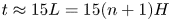 $t\approx 15 L = 15(n+1)H$. As observed in figure 6, after the flux begins to decrease in the homogeneous cell, the horizontally averaged concentration
  $\bar {c}(z,t)$ becomes roughly constant in depth,
  $\bar {c}(z,t) \approx \bar {C}(t)$, apart from in a thin boundary layer at the upper boundary of the domain. In other words, the dynamics of convection in the interior of the domain must be able to adjust and redistribute solute through the domain on a faster time scale than that at which the flux decays, so that the system evolves in a quasi-static manner.
Given these observations, the integral of the transport equation (2.9) yields a condition of global conservation of solute
 \begin{equation} L \frac{{{\rm d}} {\bar{C}}}{{{\rm d}} {t}} = F(t), \end{equation}
where  $F(t) \sim (1-\bar {C})/\delta$ is the flux through the upper boundary, given here in terms of the local boundary-layer thickness
  $\delta (t)$ (see figure 7a). This simple model is closed by specification of
  $\delta$. To achieve this, we appeal to a classical Howard–Malkus ‘critical boundary-layer depth’ argument (Malkus Reference Malkus1954; Howard Reference Howard1972), which we expect to be valid when
  $H \ll 1$. According to this argument, which was developed for unconfined fluid (as opposed to porous) convection, the thin diffusive boundary layer is maintained at a statistically steady depth that is controlled by the constraint of local stability: diffusion acts to increase the depth of the layer, but vigorous convection in the interior of the domain rapidly scours away any growth of the layer beyond a critical depth. Applied to the present situation, given that lengths have been scaled by the global concentration difference in (2.5a–c), this argument suggests that
 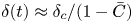 $\delta (t) \approx \delta _c/(1-\bar {C})$ and so
 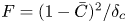 $F = (1-\bar {C})^{2}/\delta _c$, where
  $\delta _c$ is a constant. For comparison, in its classical form applied to an unconfined fluid the argument would predict
 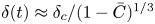 $\delta (t) \approx \delta _c/(1-\bar {C})^{1/3}$ and
  $F = (1-\bar {C})^{4/3}/\delta _c$.


Equation (4.1) can thus be integrated to yield
 \begin{equation} 1-\bar{C}(t) = \left[1 + \alpha_0 t/L\right]^{{-}1},\quad F = \alpha_0 \left[1 + \alpha_0 t/L\right]^{{-}2}, \end{equation}
where we have introduced  $\alpha _0 \equiv 1/\delta _c$ for notational convenience. Following Hewitt et al. (Reference Hewitt, Neufeld and Lister2013), we have set
  $\bar {C}(t=0) = 0$ and we adopt
  $\alpha _0 \equiv 1/\delta _c = 0.028$, which was found to give good agreement with numerical computations. (In fact,
  $\alpha _0$ is not a free fitting parameter: this value was extracted from comparison of this evolving system with the relationship between the Nusselt number (dimensionless flux) and Rayleigh number in a statistically steady cell; see e.g. Hewitt Reference Hewitt2020.) Predictions of this model are compared with data in the following section.
4.2. The limit of very high impedance
If  $\varOmega \gg 1$, the impedance can instead inhibit any advective flow across the layers, and the only solute transport across the layers is by diffusion. Initially, as discussed in § 3.3, the flux again fluctuates around a constant value
  $F \approx 0.017$, but the first low-permeability layer provides a barrier to flow and the flux begins to decrease once
  $t \approx 15 H$. After this time, we expect the system to evolve towards a step-like profile in which thin diffusive boundary layers develop on either side of each low-permeability layer in order to transport flux across the layer as efficiently as possible (as observed in figure 6).
Provided the time scale of the internal convective flow between each layer is much faster than the time scale over which the flux decays, then we might imagine that after some time this system will resemble a series of stacked, statistically quasi-steady regions (see figure 7b), each bounded above and below by a thin boundary layer, and each with a horizontally averaged concentration in the interior that is roughly independent of depth. Conservation of concentration in the regions between each low-permeability layer yields
 \begin{equation} H\frac{{{\rm d}} {\overline{C}_i }}{{{\rm d}} {t}} = F_{i-1} - F_{i} = \alpha_{i-1} ({\rm \Delta} C_{i-1})^{2} - \alpha_{i}({\rm \Delta} C_{i})^{2}, \end{equation}
for  $i=1, 2,\ldots n+1$. Here,
  $\overline {C}_i(t)$ is the interior concentration in the
  $i$th region (that is, in the region above the
  $i$th layer; see figure 7b),
  $F_i$ is the flux across the
  $i$th layer, with
  $F_0 \equiv F$ being the flux through the upper boundary and where
 \begin{equation} {\rm \Delta} C_{i} = \left\{\begin{array}{@{}cc} 1 - \overline{C}_1, & i=0, \\ (\overline{C}_{i} - \overline{C}_{i+1})/2, & 1 \leq i \leq n, \\ 0 & i \geq n+1, \end{array}\right. \end{equation}
is the difference between the bulk concentration above the  $i$th low-permeability layer and the mean concentration at that layer (figure 7b). In the second equality of (4.3) we have used the same relationship with the statistically steady cell as discussed in the previous subsection, with
  $F_i = \alpha _i ({\rm \Delta} C_{i})^{2}$, where
  $\alpha _i$ is a constant given by the reciprocal critical boundary-layer depth. The set of
  $n+1$ ODEs specified in (4.3) have initial condition
  $\overline {C}_i(t_0) = 0$ at a virtual origin
  $t=t_0$, which, as above, we set to be zero. The constants
  $\alpha _i$ are not all free parameters: indeed, one might assume that they must all be equal, since the convective processes at each layer are the same. There is, however, a difference between the upper boundary and the internal layers: at the former, the concentration is uniform, whereas at the latter the concentration can vary laterally, which allows for an enhancement to the flux. As such, while for consistency we must take
  $\alpha _0 = 0.028$ to be the value for the homogeneous cell as discussed in the previous subsection, we set the remaining values to be
  $\alpha _i = \xi \alpha _0$,
  $i\geq 1$, with a single fitting parameter
  $\xi > 1$ to describe the enhancement of the flux from varying concentration along the layers. Numerical solutions suggest
  $\xi \approx 2$, and we use that value here.
It is straightforward to integrate (4.3) numerically, but more instructive to explore the leading-order behaviour analytically. The constraint of global solute conservation follows from taking the sum of all  $n+1$ equations in (4.3)
 \begin{equation} H \frac{{{\rm d}} {}}{{{\rm d}} {t}} \sum_{i=1}^{n+1} \overline{C}_i \approx \frac{{{\rm d}} {}}{{{\rm d}} {t}} \int_{{-}L}^{0} \bar{c}(z,t)\,{{\rm d}}{z} = F = \alpha_0 \left({\rm \Delta} C_0\right)^{2}. \end{equation}
The behaviour of this model will depend on whether the concentration has reached the base of the domain or whether there are some regions that still contain unsaturated fluid. Assuming that all the  ${\rm \Delta} C_i$ evolve at the same rate to leading order, we set
  ${\rm \Delta} C_i(t) \sim A t^{\gamma }$ for some
  $A$ and
  $\gamma$, such that the total concentration in any region is
  $\overline {C}_i = 1 - 2\sum _{j=1}^{i-1} {\rm \Delta} C_j - {\rm \Delta} C_0 \sim 1 - (2i-1)A t^{\gamma }$. Any regions deeper than layer
  $N \sim (A t^{\gamma })^{-1}/2$ will thus be empty of solute, as long as
  $N< n+1$. In this limit, for
  $t\gg 1$ (4.5) reduces to
 \begin{equation} H \frac{{{\rm d}} {}}{{{\rm d}} {t}} \sum_{i=1}^{N} \overline{C}_i \sim H \frac{{{\rm d}} {}}{{{\rm d}} {t}} \left(\frac{1}{2At^{\gamma}} \right) \sim \alpha_0 A^{2} t^{2\gamma}. \end{equation}
This balance requires that  $\gamma = -1/3$,
  $A \sim (H/6\alpha _0)^{1/3}$ and
 \begin{equation} {\rm \Delta} C_i \sim \left(\frac{H}{6 \alpha_0 t}\right)^{1/3},\quad F \sim \left(\frac{ \alpha_0 H^{2}}{ 36 t^{2}}\right)^{1/3}. \end{equation}
 Alternatively, if the concentration has spread to the base of the domain at  $z=-L$, which occurs when
  $N = n+1$ or
  $t \sim [2 A (n+1) ]^{-1/\gamma } \sim 4 (n+1)^{3} H/ (3\alpha _0)$, then concentration can no longer spread into unsaturated fluid ahead, and the decay of the flux increases. In this limit, (4.5) instead reduces to give a leading-order balance
  $- H \gamma (n+1)^{2} A t^{\gamma -1} \sim \alpha _0 A^{2} t^{2\gamma }$ for
  $n, t\gg 1$, or
 \begin{equation} {\rm \Delta} C_i \sim \frac{H (n+1)^{2} }{\alpha_0 t},\quad F \sim \frac{H^{2} (n+1)^{4}}{\alpha_0 t^{2}}. \end{equation}
 Figure 8 compares predictions of both this model and the model for a homogenous medium from the previous section with numerical results. In the homogeneous case, after an initial rapid decay from the constant value, the flux decreases in excellent agreement with the model prediction, and gradually approaches the asymptotic scaling  $F \sim t^{-2}$ (4.2a,b). In the high-
 $\varOmega$ limit, the flux begins to decay earlier, as discussed above, but again after an initial rapid decay it gives excellent agreement with the model, approaching the scaling
  $F \sim t^{-2/3}$ predicted in (4.7a,b). The figure also shows results of simulations at an intermediate value of
  $\varOmega$, which are discussed in the following section.

Figure 8. The flux  $F(t)$ through the upper boundary for (a)
  $[H,n]=[5\times 10^{3},8]$, (b)
  $[H,n]=[10^{4},4]$ and (c)
  $[H,n]=[10^{4},2]$, with
  $\varOmega = 0$ (blue),
  $\varOmega = 6.4 \times 10^{4}/H$ (green) and
  $\varOmega = 1.02 \times 10^{6}/H$ (grey). The horizontal dotted line gives the flux in an unbounded homogeneous domain. The predictions of the model for a homogeneous medium (black dashed) and for
  $\varOmega \gg 1$ (red dashed) are also shown, together with some representative scalings.
The time  $t\sim 4 (n+1)^{3} H/(3\alpha _0)$ at which we expect a transition to the scalings in (4.8a,b) is too large for the length of the simulations in figure 8(a,b), but the start of this transition can be observed in figure 8(c) where
  $n$ is smaller. Note that this final decay of the flux has the same dependence on
  $H$ and
  $t$ as the homogenous model in (4.2a,b) (recalling that
  $L=(n+1)H)$. In the high-
 $\varOmega$ limit, however, the flux contains an additional factor of
  $(n+1)^{2}$, and so is larger than the homogeneous flux at late times, as can be seen in figure 8(c).
4.3. Advective reorganisation
We observed in figure 5(a) that for intermediate values of  $\varOmega$ the flux begins to decay following the same trajectory as simulations with higher impedance, but there is a qualitative change in the flux after some critical time,
  $t_c(\varOmega,H)$. After this the flux either increases or decreases at a much slower rate, before then beginning to decay again. The same feature can be seen clearly in figure 8, which includes a simulation at an intermediate value of
  $\varOmega$ and shows explicitly that the initial decay of the flux follows the high-
 $\varOmega$ theory. We have previously identified this change in the flux as the result of a reorganisation of the flow to enable appreciable advective transport across the low-permeability layers.
4.3.1. Conditions for reorganisation
Snapshots like those in figures 3 and 4 reveal something of the structure of the reorganised flow. Unlike the flow in the high- $\varOmega$ limit, which involves convective mixing in the regions between each layer, with diffusive transport across boundary layers at each layer, the reorganised flow takes the form of large plumes that propagate down across multiple layers. Dense downwelling plumes spread out and pool above each low-permeability layer, and, for high enough
  $\varOmega$, the underside of each layer is unstable to small protoplumes which carry solute back in towards the centre of each plume. Buoyant upwellings show the converse behaviour, pooling below each low-permeability layer. The signature of this dynamics is clear in the horizontally averaged concentration in figure 6, where the reorganised flow structure leads to a z-shaped profile in
  $\bar {c}$. Note that if the width of the large plumes is greater than the distance between layers
  $H$, the upper region (above the first low-permeability layer) has to adopt a slightly different flow structure from the rest of the domain (see figure 4), because the flow has to reorganise to satisfy the boundary conditions on the upper boundary.
The somewhat complicated structure of the reorganised flow means that it is not straightforward to develop a complete reduced model of the process. Instead, we provided some simple scaling balances that identify the key features of why and in what manner the flow reorganises, and demonstrate that the predictions of these balances give good agreement with numerical observations.
In order to drive flow across the low-permeability layers, the jump condition  $w \sim [p]/(\varOmega H)$ (2.15) must be satisfied. That is, if
  $\varOmega H$ is large, then a large pressure difference
  $[p]$ must be generated across the layer. From the description of the reorganised flow, it is clear that this is achieved by the build up of a large hydrostatic pressure at each layer, which in turn drives substantial lateral flow as a gravity current – hence the pooling of dense fluid above each layer. The question of when the flow is able to reorganise to adopt this structure can thus be reposed as when it is able to build up a sufficiently large hydrostatic pressure difference to make advection, rather than diffusion, a more favourable means of transport across the low-permeability layers.
For a moderate value of  $\varOmega$, the flux begins to shutdown as the first low-permeability layer blocks flow across it. Over time, the flux, and thus the driving concentration difference across the layer
  ${\rm \Delta} C_1$, decrease. However, the total available buoyancy above the layer (relative to the unsaturated ambient) is
  $\overline {C}_1$, which builds up over time and may, at some point, become large enough to drive flow over the layer. Of course, the unsaturated ambient fluid may, by that time, be located far below the upper layer as the step-like diffusive profile sketched in figure 7(b) may have spread across several layers. Nevertheless, the flow appears to be able to reorganise over many layers, and in so doing is able to bring up fresh ambient fluid from far below to the first layer, and thus to maintain a large pressure difference across all the layers (compare, for example, the region below the first layer in the upper and lower snapshots in figure 4, where fresh fluid clearly encroaches after reorganisation).
This explanation is not a complete description of the dynamics of the reorganised flow, but it allows for identification of the key balances that should determine the onset time  $t_c$. We expect the flow to reorganise if the advective flux across the layers can become comparable to the diffusive flux
  $F \sim ({\rm \Delta} C_0)^{2}$. The advective flux across the first layer scales like
  $w c$, where
  $w \sim [p]/(\varOmega H)$ and
  $c$ is the concentration scale in the region
  $c \sim \overline {C}_1 \sim 1-{\rm \Delta} C_0$. As noted above, the pressure difference will also drive lateral flow
  $u$ as a gravity current over a range
  $x$ with
  $u \sim [p]/x$, and we return to this point in the discussion of lateral scales below. If the pressure is hydrostatic, then
  $[p] \sim c z \sim (1-{\rm \Delta} C_0) z$, which will be maximised when the current fills the layer and
  $z \sim H$. Thus, the maximum advective flux that can be achieved by this flow is
  $wc \sim \varOmega ^{-1} (1-{\rm \Delta} C_0)^{2}$, and we expect flow reorganisation if
 \begin{equation} \left(1-{\rm \Delta} C_0\right)^{2} \gtrsim a \varOmega {\rm \Delta} C_0^{2}, \end{equation}
for some proportionality constant  $a$. Equivalently,
 \begin{equation} {\rm \Delta} C_0 \lesssim \frac{(a\varOmega)^{1/2} - 1}{a\varOmega - 1}\quad \text{or}\quad \overline{C}_1 \gtrsim (a\varOmega)^{1/2} \left[\frac{(a\varOmega)^{1/2}-1}{(a\varOmega) - 1}\right]. \end{equation}
 In order to compare with these predictions, we extract the onset time  $t=t_c(\varOmega,H)$ and corresponding mean concentration
  $\overline {C}_1 = \overline {C}_c$ above the first low-permeability layer from simulations as demonstrated in figure 9. The increased advective flux associated with this reorganisation occurs over some time period: to capture this, we define the onset time as the time at which the advective flux across the first layer reaches half of its subsequent maximum value, with error bars given by the time over which it rises from
  $1/4$ to
  $3/4$ of this value.

Figure 9. (a) Flux  $F(t)$ and (b) mean concentration
  $\overline {C}_1$ in the region above the first low-permeability layer for
  $H =5\times 10^{3}$ and
  $n=8$, showing the extracted time at which the flow reorganises, as defined in the main text. Data shown for
  $\varOmega = 0$ (black, for reference) and
  $\varOmega = [0.8,3.2,12.8,51.2]$ (blue, red, green, grey, respectively). All data are the ensemble average of three repeat simulations.
Figure 10 shows these data extracted from simulations with a range of  $\varOmega$,
  $H$ and
  $n$, and compared with the prediction of (4.10). Given the simplicity of the model outlined here, we find a surprisingly good fit for
  $\overline {C}_c$ across all the data when the constant of proportionality is
  $a=1$ (figure 10a). We can also predict the onset time
  $t_c$ by taking
  ${\rm \Delta} C_0$ from (4.10) and inverting the high-
 $\varOmega$ theoretical model in (4.3). Predictions of
  $t_c$ are again reasonable across the whole range of data (figure 10b). The predictions become slightly less accurate for small
  $\varOmega$, where the reorganisation of the flow is less pronounced and less well defined, and for small
  $H$, which limit violates the model assumptions in (4.3).

Figure 10. (a) The critical mean horizontally averaged concentration  $\overline {C}_c$ above the first low-permeability layer, above which advection affects the heat transport across the layers, and (b) the corresponding onset time
  $t_c$. Symbols are taken from simulations (in all cases, ensemble averaged over three repeat simulations) with
  $[H,n]=[1.25 \times 10^{3},8]$ (blue circles),
  $[H,n]=[2.5\times 10^{3},8]$ (red crosses),
  $H = 5 \times 10^{3}$ with both
  $n=2$ and
  $n=4$ (green squares) and
  $H=10^{4}$ (grey stars) with both
  $n=2$ and
  $n=4$, for
  $\varOmega H = [4,16,64,256] \times 10^{3}$. The theoretical predictions (with
  $a=1$) are given by the black (using the actual solution of the ODE in (4.3)) and red dashed (using the leading-order scaling to give (4.11)) lines.
The figure also shows the asymptotic prediction for  $t_c$ (red dashed line) which follows from the scalings in (4.7a,b)
 \begin{equation} t_c \sim \frac{H}{6\alpha_0} \left[ \frac{\varOmega - 1}{\varOmega^{1/2} -1} \right]^{3}, \end{equation}
such that  $t_c \sim H \varOmega ^{3/2}/(6\alpha _0)$ for
  $\varOmega \gg 1$.
4.3.2. Subsequent evolution
During the reorganisation of the flow, large-scale dense plumes move down through the entire domain, driving the return flow of ambient fluid. As noted above, the dense plumes have a large lateral length scale and spread over each low-permeability layer as a gravity current, allowing for sufficient build-up of pressure to drive the flow across each layer. The flux in general increases during this process, until the dense plumes have reached the base of the domain and the supply of ambient fluid is used up. After this point, the flux decays rapidly (see, e.g. figure 9), seemingly following the same scaling  $F \sim t^{-2}$ as the homogenous case described in § 4.1. This feature represents the fact that, like in the homogeneous limit, the flow shuts down in a quasi-static manner: reorganisation of the flow through the interior is rapid relative to changes in
  ${\rm \Delta} C_0$, or, equivalently, the mean concentration in the domain evolves at the same rate as
  ${\rm \Delta} C_0$. As such, (4.1) together with
  $F \sim ({\rm \Delta} C_0)^{2}$ yields the scaling
  $F \sim t^{-2}$ directly.
In fact, the decay of the flux in this regime can be more quantitatively captured by introducing the concept of an effective bulk permeability for the medium. It is well known that for simple uni-directional pressure-driven flow in a porous medium through a series of layers of differing permeability, the effective permeability  $K_{{eff}}$ of the medium is given by the harmonic mean of the individual permeabilities, weighted by the corresponding layer depths (Woods Reference Woods2015). For the problem in hand, this is
 \begin{equation} K_{{eff}} = \frac{H(1+\epsilon_H)}{H + \left(\epsilon_H H / \epsilon_K\right)} = \frac{1}{1+\varOmega} + O(\epsilon_H). \end{equation}
The effective permeability is based on the idea of pressure-driven flow across layers, and so we would not expect it to be a relevant measure while the flow is localised to the region above the first low-permeability layer, or while diffusion across the layers is important. After reorganisation, however, the flow takes the form of interleaving plumes being driven across a series of layers, which, while still being substantially more complex than the idealisation of unidirectional flow, might be better described by this construction. Given the dimensional scalings with  $K$ for velocity, time and depth in § 2.2, we can rescale the predictions for the evolution of the flux in a homogeneous medium in § 4.1, using
  $K_{{eff}}$ to compare with numerical results for different
  $\varOmega$.
Figure 11 shows this comparison. As expected, for non-zero impedance the prediction is extremely inaccurate and substantially underestimates the true flux until well after the reorganisation process has taken place. However, while the numerical results have not been run for long enough to make a clear comparison in all cases, the figure suggests that the eventual decay of the flux after reorganisation becomes reasonably well captured by this simple averaging process.

Figure 11. The flux through the upper boundary for  $[H,n]=[5\times 10^{3},8]$ compared with predictions for a homogeneous medium with an effective bulk permeability
  $K_{\text {eff}} = 1/(1+\varOmega )$ (red dashed) using the theory in § 4.1. Predictions combine a constant initial flux with the shutdown prediction of (4.2a,b); rescaling for different
  $K_{{eff}}$ takes account of the permeability scales in the flux (i.e. velocity), time and domain depth identified in § 2.2 to give, over the shutdown range,
  $F = \alpha _0 K_{{eff}} [1 + \alpha _0 K_{{eff}} t/L]^{-2}$; (a)
  $\varOmega = 0$, (b)
  $\varOmega = 0.4$, (c)
  $\varOmega = 1.6$, (d)
  $\varOmega = 6.4$ and (e)
  $\varOmega = 25.6$.
4.3.3. Lateral structure of the reorganised flow
As noted in § 4.3.1, the pressure difference  $[p] \sim w \varOmega H$ that drives flow across the low-permeability layers also drives lateral flow
  $u \sim [p]/x$ over a length scale
  $x$. These flows are linked by mass conservation:
  $u \sim wx/z$, and so we expect a lateral scale for the plumes of
 \begin{equation} x \sim \sqrt{\varOmega H z} \sim \sqrt{\varOmega} H, \end{equation}
assuming, as before, that the vertical scale  $z$ for the lateral flow is set by the depth
  $H$ of the regions between each layer. This scale can become very large – in particular, much larger than the distance
  $H$ between layers. Interestingly, the prediction here does not depend on the driving concentration difference, which suggests that the wavelength of the plumes may not evolve further as the flow shuts down.
Figure 12(a,b) shows a measure of the wavelength  $\lambda$ of plumes crossing the first low-permeability layer over time, extracted from the dominant wavenumber of a horizontal Fourier transform of
  $w$ along the layer. In the homogeneous case, the wavelength increases continually as the flux shuts down. For non-zero
  $\varOmega$, the wavelength also appears to increase after
  $t_c$ as the flow is reorganised, but the data suggest that it approaches a constant value, rather than continuing to increase. This figure also shows clearly that the lateral scales increase with
  $\varOmega$, and can become orders of magnitude larger than the corresponding scales of the plumes in a homogeneous medium.

Figure 12. (a,b) The dominant horizontal wavelength  $\lambda (t)$ of the vertical velocity
  $w$ across the first low-permeability layer, together with the onset time
  $t_c$ (stars), for (a)
  $[H,n] = [5\times 10^{3},8]$ and (b)
  $[H,n] = [10^{4},4]$. In both cases, lines show
  $\varOmega = H^{-1} [0,4,16,64] \times 10^{3}$ (black squares, blue, red, green, respectively), and all points are ensemble averaged over three repeat simulations. (c) The final wavelength
  $\lambda$, ensemble averaged over three repeat simulations, with the predicted scaling
  $\lambda \sim \sqrt {\varOmega } H$ (dashed) and a fitted prefactor of
  $3$. Data are taken from simulations with
  $H = [2.5,5,10]\times 10^{3}$ (blue, red, green, respectively), different values of
  $n$ and
  $\varOmega H = [1,4,16,64] \times 10^{3}$. The error bars follow from the assumption that horizontal mode restriction could lead to an error of
  $\pm 1$ in the number of plumes in the domain; large error bars for large
  $\sqrt {\varOmega } H$ indicate that the wavelength is comparable to the width of the domain in these simulations.
The final value of  $\lambda$ is shown in figure 12(c) for a range of
  $H$,
$H$,  $\varOmega$ and
  $n$, and it increases with
  $\sqrt {\varOmega } H$ in reasonable agreement with the theoretical prediction in (4.13). There are two important caveats that should be mentioned here. First, these lateral scales become extremely large for large
  $\varOmega$ and
  $H$, and so mode restriction could play a large role in the simulations, as reflected by the substantial error bars in the figure. Second, the final value of
  $\lambda$ was extracted from the end of each simulation, and although in most cases it appears that the lateral scale has converged towards a constant value, this is not always the case (see e.g. one of the curves in figure 12a). Nevertheless, the rough agreement with the theoretical scaling lends further credence to the simple scaling balances behind (4.13).
4.3.4. Limits on  $\varOmega$: when does reorganisation occur?

The balance in (4.10) also provides constraints on when  $\varOmega$ is too big for reorganisation to ever occur, and on when
  $\varOmega$ is too small to have any appreciable impact on the flow. For the former case, we expect that transition will always occur as long as fresh ambient fluid remains available in the domain, as the diffusive flux is continually decreasing. If, however, the concentration front has already reached the base of the domain, then there is no more unsaturated ambient fluid and the maximum available density difference in the domain will begin to drop. If this occurs, the system will simply continue to evolve following the high-
 $\varOmega$ model in (4.3) and the flux will decay according to (4.8a,b). From that model, assuming
  $n\gg 1$, concentration reaches the base of the domain over a time
  $t \sim 4(n+1)^{3} H/(3\alpha _0)$, at which point
  ${\rm \Delta} C_0 \sim [2(n+1)]^{-1}$. So we expect no transition if
 \begin{equation} \frac{\varOmega^{1/2}-1}{\varOmega-1} \lesssim \frac{1}{2(n+1)}\quad\text{or}\quad \varOmega \gtrsim (2n+1)^{2}. \end{equation}
Figure 13 shows example results for different values of  $n$ which lie on either side of this bound, demonstrating that the simulations with a lower
  $n$ follow the model prediction for the high-
 $\varOmega$ limit, whereas those with higher values of
  $n$ undergo a reorganisation of the flow.

Figure 13. The flux for  $H=2.5 \times 10^{3}$,
  $\varOmega = 25.6$ and
  $n=8$ (black),
  $n=4$ (blue) and
  $n=2$ (red), ensemble averaged over two repeat simulations, together with the prediction of the high-
 $\varOmega$ model in each case (dotted). There is no reorganisation of the flow in the case with
  $n=2$.
Conversely, we expect that  $\varOmega$ will not have an appreciable influence on the flow if the value of
  ${\rm \Delta} C_0$ predicted in (4.10) is larger than the concentration difference that drives convection in an unbounded domain (or, equivalently, if the onset time
  $t_c$ predicted is less than
  $15H$). From figure 10, we find this to occur if
  $\varOmega \lesssim 0.13$, and so we expect values of
  $\varOmega$ below this bound will have only a negligible impact on the flow.
5. Summary and discussion
5.1. Summary
This paper has explored the behaviour of convection driven by a dense source at an upper boundary in a two-dimensional porous medium that is interspersed with a series of regularly spaced, thin, horizontal low-permeability layers. The effect of the thin layers was parameterised by their impedance  $\varOmega$, with low impedance describing very thin or relatively permeable layers, and high impedance describing fatter or less permeable layers. For sufficiently low impedance the layers have negligible effect on the flow. For higher impedance, the layers can provide a buffer to flow, leading to a reduction in the strength of convection. In general, over time the flow may be able to reorganise to drive advective flow in interleaving columns across the layers, leading to a transient flattening, or even increasing, of the flux, before it again begins to reduce as the fresh fluid in the domain is used up and the convection gradually ‘shuts down’. If the impedance is sufficiently large, this reorganisation may never occur; instead, slow diffusive transport across the layers gradually fills the whole domain with dense fluid. We have explored these different regimes of flow, developed reduced models for the evolution of the convective flux in each case, identified bounding parameter groupings and times between the different regimes, and considered the spatial scales of the evolving flow. Some of these results are summarised in the phase diagram shown in figure 14, discussed in the following subsection.

Figure 14. A phase diagram showing approximate scalings for the convective flux  $F$ over time in a domain with
  $n$ layers and total depth
  $L=(n+1)H$, valid for
  $H\gg 1$ (and illustrated here for
  $n=5$). Before the flow reaches the first layer, the flux is statistically constant (white region). If the impedance
  $\varOmega$ is sufficiently small, the layers have a negligible impact on the flux, which only decreases once the flow fills the domain (red region; § 4.1). For large
  $\varOmega$ (grey regions; § 4.2), the layers act as impermeable barriers to flow, permitting only diffusive transport across them; eventually the flow reaches the base of the domain (darker grey), leading to a change in the scalings of the flux. For intermediate values of
  $\varOmega$, the flow undergoes an advective reorganisation from this impermeable regime (blue region; § 4.3) after a time
  $t = t_c \sim H [(\varOmega -1)/(\sqrt {\varOmega }-1) ]^{3} /(6\alpha _0)$ (4.11), ultimately leading to an advection-dominated regime in which the flux can be approximated using an effective permeability (darker blue).
The set-up in this study is clearly idealised, in order to explore the effect of thin, low-permeability layers on evolving convective flow. There are various ways in which this work could be extended. Perhaps the most valuable extension would be comparison with analogue laboratory experiments. Beyond this, the effect of sloping layers or a third dimension could be explored, while it would also be instructive to explore how the description of the thin layers in terms of an impedance alone breaks down as their depth is increased.
We have assumed here that the porosity and diffusivity are unaffected by the low-permeability layers. In a geological setting this may well be a reasonable assumption: the permeability of a thin layer may be many times lower than the ambient value simply because the pore length scale is much smaller; the porosity itself – and effective diffusivity – may be unchanged. Nevertheless, it is interesting to consider more generally how a change in porosity in the low-permeability layers might affect the results of this work. On first consideration, it seems likely that the effect of such variation would be small relative to the associated change in permeability: the jump condition in (2.15) and the associated advective transport across the layers would be unaffected by a change in porosity, and it would only be the diffusive flux across the layers that would decrease because of a reduction in porosity there. Thus for small or moderate impedance, when transport across the layers is dominated by advection, the impact of a change in porosity should be small. For larger impedance, however, where diffusion across the layers is important, a change in diffusive flux could cause appreciable quantitative changes to the evolution of the system over long times. Detailed exploration of the impact of porosity or diffusivity change in the low-permeability layers is left for further study.
Finally, it is worth noting that in field settings, low-permeability baffles are often also cracked and broken, creating discrete high-permeability pathways for fluid transport across them; the relative contribution to buoyancy transport across extended regions of low permeability or narrow higher-permeability patches is not obvious, and would be an interesting future study.
5.2. Discussion and simple physical implications
In a given physical situation (say, a layered sedimentary aquifer in which one intends to sequester CO $_2$), the two limits discussed in § 4.3.4 allow for an easy estimate of whether the impedance of a series of layers will be large enough to have any effect on convection, or whether it will be so large that convection across layers will never develop and the density will adopt a step-like structure as in figure 7(b). Assuming that it is possible, at least roughly, to characterise the aquifer by some number
  $n$ of thin, horizontal layers that are approximately a factor
  $\epsilon _H$ thinner than the mean vertical distance
  $H^{*}$ between them, and approximately a factor
  $\epsilon _K$ less permeable than the bulk permeability
  $K^{*}$ of the medium, one can compute a measure of the impedance
  $\varOmega = \epsilon _H/\epsilon _K$.
Figure 14 shows a phase diagram that summarises the behaviour of the flux over time for different  $\varOmega$. We see that the former situation of negligible impact (red region in the figure) will occur if
  $\varOmega \lesssim 0.13$, while the latter situation (grey region) will persist forever if
  $\varOmega \gtrsim (2n+1)^{2}$. In each case the evolution of the flux will be given by the models outlined in § 4. If
  $\varOmega$ lies between these two bounds, then there will be some transient depletion in the strength of convection owing to resistance from the thin layers, followed by a reorganisation of the dynamics to allow for flow across the layers; this will occur after a time
  $t_c$ shown in figure 14 by the solid blue curve. The eventual decay of the flux after this reorganisation can be roughly determined by ‘coarse graining’ the problem to treat it as a homogeneous medium with an effective bulk permeability
  $K^{*}/(1+\varOmega )$ (although such a description is wildly inaccurate at earlier times; see § 4.3.2). The main phenomenological feature of the reorganised flow would be the development of a large lateral length scale
  $x^{*} \sim 3 \varOmega ^{1/2} H^{*}$ between counterflowing dense and buoyant plumes (see § 4.3.3). This length scale depends intrinsically on
  $H^{*}$, which reflects its basis in the local dynamics driving lateral flow in the regions between each low-permeability layer (in contrast to the description of the flux in terms of an effective permeability, which does not depend on
  $H^{*}$). The results of this work suggest that this lateral scale may not continue to evolve as convection shuts down, raising the intriguing possibility that historic convective processes might leave some signature in the geological record that could be observed.
Declaration of interests
The author reports no conflict of interest.


 Open access