


Crossref Citations
This article has been cited by the following publications. This list is generated based on data provided by Crossref.
Tambe, Sumit
Kato, Kentaro
and
Hussain, Zahir
2024.
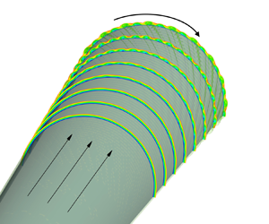
Görtler-number-based scaling of boundary-layer transition on rotating cones in axial inflow.
Journal of Fluid Mechanics,
Vol. 987,
Issue. ,
Bhoraniya, Ramesh
Thummar, Mayank
and
Hussain, Zahir
2024.
Modal and nonmodal global instabilities of rotating incompressible axisymmetric boundary layer.
Computers & Fluids,
Vol. 285,
Issue. ,
p.
106459.
DePei, SONG
ChangPing, YU
and
XinLiang, Li
2024.
Stability and transition of hypersonic boundary layer flow over a rotating blunt cone.
SCIENTIA SINICA Physica, Mechanica & Astronomica,
Vol. 54,
Issue. 10,
p.
104703.
Song, Qinyang
Dong, Ming
Zhao, Lei
Chu, Xianying
and
Wu, Ningning
2024.
Influence of spanwise wall vibration on non-modal perturbations subject to freestream vortical disturbances in hypersonic boundary layers.
Journal of Fluid Mechanics,
Vol. 999,
Issue. ,