


Crossref Citations
This article has been cited by the following publications. This list is generated based on data provided by Crossref.
García, Edgardo
Hussain, Fazle
Yao, Jie
and
Stout, Eric
2025.
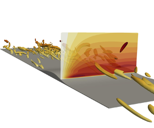
Wall turbulence perturbed by a bump with organized small-scale roughness: coherent structure dynamics.
Journal of Fluid Mechanics,
Vol. 1006,
Issue. ,