2.1. Description of PCP flow

We consider only the special case for PCP flow where the velocity-difference vector is aligned with the externally applied pressure gradient. In Cartesian coordinates $(x,y,z)$ with $y$ wall-normal, $x$ streamwise and $z$ spanwise, the parallel plane walls are at $y=\pm h$. The flow configuration is shown in figure 1, where the lower/upper walls move in the $x$-direction with speeds $U_c$ and $-U_c$, respectively. The pressure-gradient vector points in the negative $x$-direction, so the mass-flow rate is positive. This configuration contains all possible PCP flows with $\phi =0$. To illustrate general flow behaviour, three sketched velocity profiles are shown. The dashed line denotes a laminar Couette flow with zero pressure gradient, the solid line profile shows zero skin friction (ZSF) on the bottom wall, and the dash-dotted line represents a Poiseuille-type flow with a stronger pressure gradient.

Figure 1. Sketch of PCP flow showing two parallel walls with separation distance $L_y=2h$. Lower and upper walls move with velocities $\pm U_c$, respectively. Negative mean pressure gradient ${\rm d}P/{{\rm d} x}$ results in a mean bulk flow with positive mass-flow rate in the $x$-direction. Sketched velocity profiles: dashed line for laminar Couette flow, solid line for flow with zero skin friction on bottom wall, and dash-dotted line for flow with stronger pressure gradient.

The flow is assumed to be statistically stationary with bulk wall-parallel mean velocity $M/(2h)$, where $M>0$ is the volume flow rate. Two independent Reynolds numbers can then be defined as

(2.1a,b)\begin{equation} Re_c = \frac{U_c h}{\nu}, \quad Re_M = \frac{M}{2 \nu} = \frac{1}{2\nu}\int^h_{{-}h}U(y)\,{{\rm d} y}, \end{equation}

where $\nu$ is the kinematic viscosity, and $U(y)$ is the streamwise mean velocity. It is convenient to work in polar coordinates $(Re,\theta )$ defined by $Re_c= Re\cos \theta$, $Re_M = Re\sin \theta$, so that

(2.2a,b)\begin{equation} Re =\sqrt{Re_c^2 + Re_M^2}, \quad \tan \theta = \frac{Re_M}{Re_c}, \end{equation}

where $Re$ is the defining Reynolds number. The PC and PP limits correspond to $\theta =0^\circ$, $\theta = 90^\circ$, respectively. If we write $Re= U_0 h/\nu$, then this defines an effective general outer velocity scale $U_0=U_c/\cos \theta = M/(2h\sin \theta )$ for PCP flow. The nominal singularity $U_c/\cos \theta$ as $\theta \to 90^\circ$ and $M/(2h\sin \theta )$ as $\theta \to 0^\circ$ is noted, but this does not compromise the utility of $U_0$ as an outer velocity over the range $\theta \in [0^\circ, 90^\circ ]$.

A specific flow is defined by given $Re$ and $\theta$. Skin-friction velocities for both walls are defined as

(2.3a,b)\begin{equation} u_{\tau,t} = \sqrt{ \nu\,|\eta_h|}{\rm sgn}({-\eta_h}), \quad u_{\tau,b} =\sqrt{\nu\,|\eta_{{-}h}|}{\rm sgn}({ \eta_{{-}h}}), \end{equation}

with $\eta _y = {{\rm d}U}/{{\rm d} y} |_{y}$ as the velocity gradient at $y$. Corresponding skin-friction Reynolds numbers are

(2.4a,b)\begin{equation} Re_{\tau,t} = \frac{u_{\tau,t} h }{\nu}, \quad Re_{\tau,b} = \frac{u_{\tau,b} h}{\nu}. \end{equation}

With these definitions, $Re_{\tau,t} >0$ for all PCP flows, while $Re_{\tau,b}<0$ for PC flow ($\theta =0^\circ$) and $Re_{\tau,b}>0$ ($\theta = 90^\circ$) for PP flow. Hence when $\theta$ increases in $(0^\circ, 90^\circ )$ at fixed $Re$, $Re_{\tau,b}$ must change sign at least once. We define flow regions in the first quadrant of the $(Re_c,Re_M)$ plane as Couette-type for $Re_{\tau,b}<0$ and Poiseuille-type for $Re_{\tau,b}>0$. The curve $Re_{\tau,b}(Re,\theta )=0$ corresponds to $\theta = \theta _c$. We refer to $\theta _c$ as the $PC \leftrightarrow PP$ critical angle. This will be seen later to be a single-valued function $\theta _c(Re)$.

Another Reynolds number based on pressure gradient can also be defined as $Re_p = (-({{\rm d}P}/{{\rm d} x}) h^3)^{1/2} /\nu$, where $P \equiv p/\rho$, with $p$ the pressure and $\rho$ the constant fluid density. Using the streamwise pressure–skin-friction balance, this can be expressed as

(2.5)\begin{equation} Re_p^2 = \tfrac{1}{2} ( Re_{\tau,t} |Re_{\tau,t}| + Re_{\tau,b} |Re_{\tau,b}| ). \end{equation}

Since, as will be seen, $Re_{\tau,t}$ and $Re_{\tau,b}$ are both functions of $(Re,\theta )$ only, $Re_p$ is also a function of $(Re,\theta )$.

2.2. Numerical methods and LES models

Simulations are reported using an incompressible Navier–Stokes solver for a channel domain with dimensions $L_x \times L_y \times L_s$ (streamwise, wall-normal and spanwise directions, respectively). Boundary conditions are spatially periodic streamwise and spanwise, with Dirichlet velocity boundary conditions on $y=\pm h$. Both DNS and LES are performed. The generically filtered incompressible Navier–Stokes equations are

(2.6)\begin{gather} \frac{\partial \widetilde{u_i}}{\partial t} + \frac{\partial \widetilde{u_i} \widetilde{u_j}}{\partial x_j} ={-}\frac{\partial \tilde{P}}{ \partial x_i} + \nu\frac{\partial^2 \widetilde{u_i}}{\partial x_j^2} - \frac{\partial T_{ij}}{\partial x_j}, \quad \frac{\partial \widetilde{u_i}}{\partial x_i} = 0, \end{gather}

(2.7)\begin{gather}\tilde{q}= \int^\infty_{-\infty} q(x')\,G(x-x')\,{{\rm d} x}', \end{gather}

where $G(\eta )$ is a general filter. Boundary conditions are

(2.8)\begin{gather} \widetilde{u_i} = (U_c+u_b,v_b,w_b), \quad \text{at the bottom wall}, \end{gather}

(2.9)\begin{gather}\widetilde{u_i} = ({-}U_c+u_t,v_t,w_t), \quad \text{at the upper wall} . \end{gather}

The DNS mode uses the unfiltered Navier–Stokes equations, while LES requires modelling for the SGS tensor $T_{ij}= \widetilde {u_iu_j}- \widetilde {u_i}\widetilde {u_j}$ with the added assumption that filtered fields are identified with computed resolved-scale fields. Explicit filtering is used nowhere presently. For DNS and WRLES, $(u_b,v_b,w_b)$ and $(u_t,v_t,w_t)$ are zero, while for WMLES, a wall model provides consistent slip velocity boundary conditions at a virtual wall. The fractional-step method is used to solve the equations with a third-order Runge–Kutta method for temporal evolution. The staggered grid strategy ensures the conservation of kinetic energy, which corresponds to a skew-symmetric form of the convective term. The pressure Poisson equation is reduced to a series of one-dimensional linear equations by Fourier expansion in the streamwise and spanwise directions. In simulations, the time step $\Delta t$ satisfies dynamically that a Courant–Friedrichs–Lewy number be unity.

For LES, $T_{ij}$ is evaluated using the stretched-vortex SGS model, which represents subgrid motion using stretched vortices in each computational cell (Chung & Pullin Reference Chung and Pullin2009), with directional unit vector $\boldsymbol {e}^v$ aligned with the principal extensional rate-of-strain eigenvector of the local resolved flow, giving

(2.10a,b)\begin{equation} T_{ij} = (\delta_{ij} - \boldsymbol{e}_i^v\boldsymbol{e}_j^v) K, \quad K=\int_{k_c}^\infty E(k)\, {\rm d}k , \end{equation}

where $K$ is the subgrid kinetic energy, and $E(\kappa )$ is the SGS energy spectrum. Closure of $E(k)$ uses the stretched-spiral vortex solution of the Navier–Stokes equation (Lundgren Reference Lundgren1982). See Chung & Pullin (Reference Chung and Pullin2009).

For WMLES, the virtual-wall model (VWM) is used (Chung & Pullin Reference Chung and Pullin2009). This consists first of an ordinary differential equation for $u_\tau (x,z,t)$ at each wall point, derived from an integration in the wall-normal direction of the local streamwise momentum equation over a thin wall-adjacent layer $0\le y \le \delta$ and given by

(2.11) \begin{equation} \frac{{\rm d} u_\tau}{{\rm d} t} = \frac{ u_\tau } {\tilde{u}|_{\delta}} \left( \left. - \frac{\partial \widetilde{uu} }{\partial x} \right|_{\delta} \left. -\frac{\partial \widetilde{uw} }{\partial z} \right|_{\delta} \left. -\frac{\partial \tilde{P} }{\partial x} \right|_{\delta} -\frac{1}{\delta} \left. \widetilde{uv} \right|_{\delta} + \frac{{\nu} }{\delta} \left. \frac{\partial \tilde{u}}{\partial y} \right|_{\delta} - \frac{1}{\delta}\,u_\tau^2 \right). \end{equation}

With $u_\tau (x,y,t)$ known, the VWM then provides a slip-velocity boundary condition at a virtual wall of $y=\delta _0<\delta$ as

(2.12)\begin{equation} \tilde{u} (\delta_0^+) = u_\tau \left( \frac{1}{\kappa} \ln \left( \frac{\delta_0^+}{\delta_\nu^+} \right) + \delta_\nu^+ \right), \end{equation}

with $\kappa = \gamma K^{1/2} u_\tau /(-2T_{xy})$ and where $\delta ^+_\nu$ is an effective offset parameter. See Chung & Pullin (Reference Chung and Pullin2009) and Saito, Pullin & Inoue (Reference Saito, Pullin and Inoue2012) for computational details and sensitivity testing. Where at a wall $u_\tau$ is very small compared with the outer velocity scale, the VWM is turned off.

2.3. Simulations performed

We report two series of simulations, the first for general PCP flow, and the second focused on a subset of flows with $Re_{\tau,b}=0$ on the bottom wall (ZSF flows). Pirozzoli et al. (Reference Pirozzoli, Bernardini and Orlandi2011) reported DNS of PCP at $Re_\tau \approx 250$ with a relatively small wall-parallel domain approximately $(L_x \times L_z) =(12{\rm \pi} h \times 4{\rm \pi} h)$. Pirozzoli et al. (Reference Pirozzoli, Bernardini and Orlandi2014) suggested that a domain $(L_x \times L_z) =(60 h \times 16 h)$ is generally required to eliminate spurious flow confinement effects, a rule generally followed in simulations by Avsarkisov et al. (Reference Avsarkisov, Hoyas, Oberlack and García-Galache2014), Lee & Moser (Reference Lee and Moser2018) and Cheng et al. (Reference Cheng, Pullin and Samtaney2022). Lee & Moser (Reference Lee and Moser2018) report that the spanwise domain has a non-negligible effect on some mean profile diagnostics, for example the velocity gradient at the channel centre, which shows an almost $20\,\%$ relative error at around $Re_\tau \approx 220$. The computational domain for all present simulations is chosen as $L_x \times L_y \times L_z = 20{\rm \pi} h \times 2h \times 6{\rm \pi} h$.

Direct numerical simulation flows include $Re=4000$, $6000$, while WRLES is implemented for $Re=10\,000$, $20\,000$. For each $Re$, $\theta =0^\circ$, $15^\circ$, $30^\circ$, $35^\circ$, $37.5^\circ$, $40^\circ$, $42.5^\circ$, $45^\circ$, $47.5^\circ$, $50^\circ$, $60^\circ$, $75^\circ$ and $90^\circ$. Simulation flow parameters are summarized in figure 2, showing both the $(Re, \theta )$ and $(Re_M, Re_c)$ planes. For each $Re$, a specific mesh is employed. For DNS at $Re=4000$ and $6000$, we have $N_x \times N_y \times N_z = 2048\times 256\times 1024$ and $N_x \times N_y \times N_z = 3072\times 320 \times 1536$, respectively. For WRLES at $Re=10\,000$, we have $N_x \times N_y \times N_z = 2048\times 128\times 1024$, while for $Re=20\,000$, we have $N_x \times N_y \times N_z = 3072\times 160 \times 1536$. For both DNS and WRLES, grid-stretching in the wall-normal direction is used as described in Cheng et al. (Reference Cheng, Pullin and Samtaney2022). For WMLES, the grid is uniform in all directions. Validation studies of both WRLES and WMLES for PC flow were conducted by Cheng et al. (Reference Cheng, Pullin and Samtaney2022), who also reported on the effect of spanwise domain size on flow diagnostics at $Re_\tau = 500$.

Figure 2. Parameters for general PCP flow: simulation points in (a) the $(Re_M, Re_c)$ plane, (b) the $(Re, \theta )$ plane. Each symbol denotes a specific simulation. Here, $Re_c= U_c h/\nu$, $Re_M = M/(2\nu )$, $Re \equiv (Re_c^2+Re_M^2)^{1/2} = U_0 h/\nu$ and $\theta = \arccos (Re_c/Re)$. Blue $\blacktriangle$ indicates DNS at $Re= 4000$ with mesh $2048\times 256\times 1024$. Red $\blacktriangledown$ indicates DNS at $Re=6000$ with mesh $3072\times 320\times 1536$. Black $\blacktriangleleft$ indicates WRLES at $Re=10\,000$ with mesh $2048\times 128\times 1024$. Blue $\blacktriangleright$ indicates WRLES at $Re=20\,000$ with mesh $3072\times 160\times 1536$.

Table 1 summarizes $Re$, the mesh resolution and the corresponding numerical methodology for ZSF flow simulations. Also shown are calculated values of $Re_{\tau,t}$. Values of both $Re_{\tau,t}$ and $Re_{\tau,b}$ reported presently were obtained as time-planar averages over a time window $\varGamma _t$, defined as $N_t \times \max (|u_{\tau,b}|,|u_{\tau,t}|) h/\nu$, consisting of many wall-transit times through the computational domain. Here, $N_t \approx 20$ for DNS, and $N_t \approx 50$ for WRLES and WMLES. Several low-$Re$ DNS cases are included in table 1, including laminar flow at $Re=100$ and $300$, and an incipient turbulent flow at $Re=1000$. Simulations reported include $Re=4000$ and $6000$ (DNS), and $Re=10\,000$ and $20\,000$ (WRLES). To access higher $Re$, WMLES were performed for $Re=10^5$, $10^6$, $10^7$, $10^8$, $10^9$ and $10^{10}$.

Table 1. Simulations for PCP flows with ZSF on the bottom wall, where $Re$ is fixed for each simulation, with $\theta$ such that the bottom-wall frictional Reynolds number is $Re_{\tau,b}\approx 0$. The final two columns show the computed top-wall frictional Reynolds number $Re_{\tau,t}$ and the ZSF angle $\theta _c$, respectively. The computational domain is $(L_x/h, L_y/h, L_z/h) = (18{\rm \pi}, 2, 6{\rm \pi} )$.

3.1. Velocity statistics at $Re=6000$

Figure 3 shows profiles in velocity-difference form to highlight changes in the near-wall velocity gradients as $\theta$ changes at fixed $Re$. Figure 3(a) shows $(U(y)-U_c)/U_0$ for flow near the bottom wall, while figure 3(b) depicts $(U+U_c)/U_0$ for flow near the upper wall. The velocity gradient on the top wall reaches a maximum at around $\theta \approx 45^\circ$, while the bottom-wall velocity gradient changes sign at $\theta \approx 37.5^\circ$, corresponding to $Re = 6000$. This is the general change from Couette-type to Poiseuille-type flow.

Figure 3. (a) Velocity $U+U_c$ in the upper-wall reference frame. (b) Mean velocity $U-U_c$ in the bottom-wall reference frame. Solid lines with blue symbols: ${\blacktriangle }$, $\theta =0^\circ$; ${\blacktriangledown }$, $\theta =15^\circ$; ${\blacktriangleleft }$, $\theta =30^\circ$; ${\blacktriangleright }$, $\theta =45^\circ$; ${{\scriptstyle \blacksquare }}$, $\theta =60^\circ$; ${\scriptstyle \blacklozenge }$, $\theta =75^\circ$; ${\bullet }$, $\theta =90^\circ$. Dashed lines with black symbols: ${\scriptstyle \blacksquare }$, $\theta =35^\circ$; ${\blacktriangle }$, $\theta =37.5^\circ$; $\blacktriangledown$, $\theta =40^\circ$; $\blacktriangleleft$, ${\theta =42.5^\circ}$.

Wall-relative mean velocity profiles for the top wall in the form $U_t^+ = (U+U_c)/u_{\tau,t}$ versus $d_t^+ = (h-y)u_{\tau,t}/\nu$ are shown in figure 4(a) for seven values of $\theta$. For flow near the bottom wall, plots of $U_b^+ = (U-U_c)/u_{\tau,b}$ versus $d_b^+ = (h+y)|u_{\tau,b}|/\nu$ in figure 4(b) show negative and positive wall-relative velocity for Couette-type and Poiseuille-type flow, respectively. The velocity gradient indicator function $\varXi (d^+)$ is shown in figure 5. Near the top wall and the bottom walls, $\varXi _t$ and $\varXi _b$ are defined respectively as

(3.1a,b)\begin{equation} \varXi_t = d_t^+\,\frac{{\rm d} U_t^+ }{{\rm d} (d_t^+)}, \quad \varXi_b = d_b^+\,\frac{{\rm d} U_b^+ }{{\rm d} (d_b^+)}. \end{equation}

In figure 5(a), all flows indicate the presence of a logarithmic region with $\varXi _t \approx 2.5$, with reasonable collapse over the whole range of $\theta$ in figure 4(a). In figure 5(b), nearly constant $\varXi _t$ regions are apparent only for $\theta$ near or at $\theta =0^\circ$ and $90^\circ$. As $\theta$ moves between these limit values, the logarithmic-like region breaks and then rebuilds during the transition from PC flow to PP flow. This can be seen clearly in the mean profiles in figure 4(b).

Figure 4. Mean streamwise velocity profiles at $Re=6000$. (a) Scaling with the upper-wall friction velocity $u_{\tau,t}$: $U_t^+ = (U+U_c)/u_{\tau,t}$, $d_t^+ = (h-y)u_{\tau,t}/\nu$. (b) Scaling with the bottom-wall friction velocity $u_{\tau,b}$: $U_b^+ = (U-U_c)/u_{\tau,b}$, $d_b^+ = (h+y)|u_{\tau,b}|/\nu$. Symbols as in figure 3. Reference log law: $U^+ = {\ln (d^+)}/{\kappa } + A$. Dashed lines indicate $\kappa =0.41$ and $A=5.1$. Dash-dotted lines indicate $\kappa =0.384$ and $A=4.27$.

Figure 5. Scaled velocity gradient $\varXi$ at $Re=6000$. (a) Scaling with the upper-wall friction velocity $u_{\tau,t}$: $\varXi _t = d_t^+\,{\rm d}(U_t^+ )/{\rm d}(d_t^+)$. (b) Scaling with the bottom-wall friction velocity $u_{\tau,b}$: $\varXi _b = d_b^+\,{\rm d}(U_b^+ )/{\rm d}(d_b^+)$. Symbols as in figure 3. Reference dashed lines: $\varXi = \pm 2.5$.

For a model log profile of the form $U^+ = {\ln (d^+)}/{\kappa } + A$, Lee & Moser (Reference Lee and Moser2015) suggested $\kappa =0.384$ and $A= 4.27$ obtained from DNS of PP flow, while Pirozzoli et al. (Reference Pirozzoli, Bernardini and Orlandi2014) found that $\kappa = 0.41$ and $A = 5$ provide a good fit for PC flow. Later DNS of PC flow by Lee & Moser (Reference Lee and Moser2018) found similar values. In figure 4(b), we use these different values for the log lines shown in the PP and PC flow limits, respectively. In figure 4(a), the PC values are used.

3.2. Turbulent kinetic energy budget at $Re=6000$

In the transition from PC flow to PP flow, the velocity deviation from the log law for some cases indicates that the flow deviates from behaviour typical of canonical wall-bounded turbulence. To evaluate the flow near the bottom wall, we investigate the turbulent kinetic energy budget. The transport equation for the turbulent kinetic energy $e = u'^2 + v'^2 + w'^2$ can be obtained by multiplying the Navier–Stokes momentum equations by $u_i$, subtracting the equation for the mean momentum equation, and taking a time-planar average. For statistically stationary flow, this can be expressed as

(3.2)\begin{equation} P + T + \varPi + D + \epsilon = 0, \end{equation}

with $P$, $T$, $\varPi$, $D$ and $\epsilon$ denoting the turbulent production, turbulent transport, pressure transport, viscous diffusion and dissipation terms, respectively. These are given by

(3.3)\begin{equation} \left. \begin{aligned} P(y) & \equiv{-}\overline{u'v'}\,\frac{{\rm d}U}{{\rm d} y}, \quad T(y) \equiv{-}\frac{{\rm d}\overline{(ev')}}{{\rm d} y}, \quad \varPi (y) \equiv{-}\frac{{\rm d}\overline{(pv'/\rho)}}{{\rm d} y},\\ D(y) & \equiv \nu\,\frac{{\rm d}^2 \bar{e}}{{{\rm d} y}^2}, \quad \epsilon(y) \equiv{-}\nu\,\overline{ \left(\frac{\partial u_i}{\partial x_j}\right)^2}, \end{aligned} \right\} \end{equation}

with the overbar referring to a plane and time average to be defined explicitly later, in (5.1a,b).

Figures 6(a,b), respectively, show profiles of these terms over the bottom half-channel for two cases: pure Couette flow $\theta =0^\circ$ and also $\theta = 37.5^\circ$, where the bottom-wall skin friction is almost zero. All are normalized on outer scales as $U_c^3h^{-1}$. Pure Couette flow displays the well-known near-wall balance of diffusion with dissipation, changing to an inertial-range balance between turbulent production and dissipation at larger wall-normal distances. For $\theta = 37.5^\circ$, all terms are reduced by an order of magnitude. A diffusion–dissipation balance is again present in the near-bottom-wall flow, while farther out, the production almost vanishes. Flow with $\theta =0^\circ$ shows a generally similar balance profile to the corresponding case reported by Pirozzoli et al. (Reference Pirozzoli, Bernardini and Orlandi2011), while our flow with $\theta = 37.5^\circ$ shows smaller production near the centreline than that of their SL (shearless) flow.

Figure 6. Turbulent kinetic energy budget near the bottom wall for $Re=6000$: (a) $\theta =0^\circ$, pure Couette flow; (b) $\theta =37.5^\circ$, with small skin-friction magnitude on the bottom wall. Red $\square$, $P$ turbulence production; blue $\circ$, $\varPi$ pressure transport; blue $\triangledown$, $T$ turbulent transport; black $\scriptstyle \triangle$, $D$ diffusion; blue $\scriptstyle \lozenge$, $\epsilon$ dissipation.

Figure 7 shows wall-normal profiles of the production–dissipation ratio $P/\epsilon$ at $Re=6000$. In figure 7(a), with $\theta$ from $0^\circ$ to $42.5^\circ$, all profiles collapse near the upper wall. Away from this wall, there is rapid increase to approximately $P/\epsilon \approx 2$, with further decrease to $P/\epsilon \sim 1$ in the inertial region. Near the bottom wall, the peak value decreases monotonically with increasing $\theta$. For $\theta = 37.5^\circ$, no obvious peaks are found, with $P/\epsilon$ increasing slowly with distance from the bottom wall. Further increasing $\theta$ gives negative $P/\epsilon$, so that production becomes negative in the near-bottom-wall region. At $\theta = 42.5^\circ$, $P/\epsilon$ again becomes positive close to the bottom wall.

Figure 7. Distribution of the ratio of turbulent production and dissipation for $Re=6000$. Each line corresponds to a different $\theta$. (a) Blue symbols: ${\blacktriangle }$, $\theta =0^\circ$; ${\blacktriangledown }$, $\theta =15^\circ$; ${\blacktriangleleft }$, $\theta =30^\circ$. Black symbols: ${\scriptstyle \blacksquare }$, $\theta =35^\circ$; ${\blacktriangle }$, $\theta =37.5^\circ$; $\blacktriangledown$, $\theta =40^\circ$; $\blacktriangleleft$, $\theta =42.5^\circ$. (b) Black symbol: $\blacktriangleleft$, $\theta =42.5^\circ$. Blue symbols: ${\blacktriangleright }$, $\theta =45^\circ$; ${{\scriptstyle \blacksquare }}$, $\theta =60^\circ$; ${\scriptstyle \blacklozenge }$, $\theta =75^\circ$; ${\bullet }$, $\theta =90^\circ$.

The appearance of negative $P/\epsilon$ over $37.5^\circ \lesssim \theta \lesssim 45^\circ$ generally represents energy transfer from unsteady fluctuations to the mean flow. This implies that the kinetic energy of the fluctuating (unsteady) flow is suppressed, and that the near-wall flow has effectively laminarized. Negative $P/\epsilon$ first appears across the ZSF boundary (see § 7 for more discussion) near $\theta =37.5^\circ$, where $\textrm {d}U/{\textrm {d} y}$ changes sign, while $\overline {u'v'}$ remains small but negative. At around $\theta \approx 42.5^\circ$, $\overline {u'v'}$ changes sign in the near-bottom-wall flow, which regenerates positive production, although the corresponding peak value of $P/\epsilon$ remains small.

Figure 7(b) shows $P/\epsilon$ profiles in the range $42.5^\circ \le \theta \le 90^\circ$. For these flows, the regenerated peak value increases from near zero to $P/\epsilon \approx 2$ at $\theta =60^\circ$. Further increase in $\theta$ leads to the re-establishment of production–dissipation balance as the near-bottom-wall flow re-transitions to a classical wall-bounded turbulent state.

3.3. Mean velocity profile near ZSF on the bottom wall

Averaging and wall-normal integration of the streamwise momentum equation in $(-h,y)$ gives the relation between the stress $\overline {u'v'}(y)$ and the mean velocity gradient as

(3.4a,b)\begin{equation} \overline{u'v'}(y) - \left. \nu\,\frac{\partial \bar{u}}{ \partial y} \right|_y ={-} S\,u_{\tau,b}^2 -\frac{{\rm d}P}{{\rm d} x}\,(y+h) ,\quad S = {\rm sgn}\left(\left.\dfrac{ {\rm d}U(y) }{{{\rm d} y} }\right|_{{-}h} \right), \end{equation}

where $S= -1$ for Couette-type flows, and $S = 1$ for Poiseuille-type flows. In obtaining (3.4a,b), possible non-homogeneity in the spanwise direction is ignored. This is not important presently, and will be discussed later. In figure 8, we plot the distribution of the Reynolds stress $\overline {u'v'}$. Figure 8(a) shows $\overline {u'v'}/u_{\tau,t}^2$ for all $\theta$ at $Re=6000$ using top-wall inner scaling, while figure 8(b) shows $\overline {u'v'}/u_{\tau,b}^2$ using bottom-wall inner scaling, for flows near $u_{\tau,b}=0$. In figure 8(a), the stress distribution near the top wall shows a collapse in inner scaling, while near but not very close to the bottom wall, the stress distribution shows a consistent tendency of decreasing magnitude, from a plateau of $\overline {u'v'}/u_{\tau,t}^2 \approx 1$ for $\theta =0^\circ$, to almost zero for $\theta \approx 40^\circ$, with further decrease to $\overline {u'v'}/u_{\tau,t}^2 \approx -1$ for $\theta =90^\circ$. This tendency is similar to the distribution of $\overline {u'v'}/U_0^2$, which is not shown presently. Near the ZSF condition, there is no observable collapse for $\overline {u'v'}/u_{\tau,t}^2$. In figure 8(b), the Reynolds stress is plotted using bottom-wall inner scaling, showing large scatter.

Figure 8. Profile of Reynolds stress $\overline {u'v'}$ versus $y/h$ for $Re=6000$: (a) $\overline {u'v'} / u_{\tau,t}^2$ for all $\theta$ flows; (b) $\overline {u'v'}/u_{\tau,b}^2$ for simulations near the ZSF flow. Symbols as in figure 3.

A near-wall close-up of figure 8(a) is shown in figure 9(a) for $\theta =40^\circ, 42.5^\circ, 45^\circ$ near but above the ZSF condition. Solid lines are the scaled right-hand side of (3.4a,b) as $( - S\,u_{\tau,b}^2 -({\textrm {d}P}/{\textrm {d}x})(y+h)) / u_{\tau,t}^2$. Up to some distance from the bottom wall, the velocity gradient term and the pressure term contribute strongly to the balance of (3.4a,b).

Figure 9. Balance of wall-normal integral of the streamwise momentum equation. (a) Equation (3.4a,b). Symbols: close-up of $\overline {u'v'}/ u_{\tau,t}^2$ for near-ZSF flows. Solid lines: $( - u_{\tau,b}^2 -({\textrm {d}P}/{\textrm {d} x}) (y+h)) / u_{\tau,t}^2$ for corresponding $\theta$. (b) Balance of (3.6). Symbols: simulation $U-U_c$ for near-ZSF flows. Solid lines: $({1}/{\nu }) ( S\, u_{\tau,b}^2 ( y+h) - (({u_{\tau,t}^2 + S\, u_{\tau,b}^2})/{4h}) (y+h)^2 )$ for corresponding $\theta$. Black symbols: $\blacktriangle$, $\theta =37.5^\circ$; $\blacktriangledown$, $\theta =40^\circ$; $\blacktriangleleft$, $\theta =42.5^\circ$. Blue symbol: $\blacktriangleright$, $\theta =45^\circ$.

Further integration of the streamwise momentum equation in $(-h,h)$ and elimination of $\textrm {d}P/{\textrm {d} x}$ from (3.4a,b) gives

(3.5)\begin{equation} \overline{u'v'}(y) - \nu\left.\frac{\partial \bar{u}}{ \partial y} \right|_y = \frac{h+y}{ 2h }\left(u_{\tau,t}^2 + S\,u_{\tau,b}^2 \right) - S\,u_{\tau,b}^2 . \end{equation}

Integration of (3.5) in $(-h,y)$ then leads to an expression for the mean velocity profile as

(3.6)\begin{equation} U(y) - U_c = \frac{1}{\nu} \left( S\,u_{\tau,b}^2 ( y+h) - \frac{u_{\tau,t}^2 + S\, u_{\tau,b}^2}{4h}\,(y+h)^2 +\int_{{-}h}^y\overline{u'v'}(\xi)\,{\rm d}\xi \right) . \end{equation}

Figure 9(b) shows the velocity profiles near the bottom wall for three cases, ${\theta = 40^\circ},\,42.5^\circ, 45^\circ$, which, from figure 8, have $Re_{\tau,b}>0$. Equation (3.6) is also plotted using $u_{\tau,t}$ and $u_{\tau,b}$ from the simulations but with $\overline {u'v'}\equiv 0$. This shows a qualitatively similar shape to simulation profiles: a near-wall peak is indicated with increasing maximum and with location that moves off from the wall with increasing $\theta$ at fixed $Re = 6000$.

In summary, with $Re$ fixed and sufficiently large for Poiseuille/Couette flow turbulence to exist, the flow near the top wall remains in a turbulent state while $\theta$ increases in $0^\circ \le \theta \le 90^\circ$. Near the bottom wall, the turbulence gradually weakens as $\theta$ is increased. Both production and dissipation reduce, with production becoming negative over a small range $37.5^\circ \lesssim \theta \lesssim 42.5^\circ$. Taken together with the loss of a log-like region, this indicates that the near-bottom-wall flow has laminarized perhaps over a range $\theta \approx 30^\circ-50^\circ$. Further increase in $\theta$ re-establishes near-bottom-wall turbulence up to the Poiseuille limit $\theta =90^\circ$. During flow laminarization, the pressure gradient effect is small for $\theta <\theta _c$, while it produces a near-wall mean velocity maximum with almost laminar flow between the maximum and the wall for $\theta >\theta _c$. Shear stresses on both walls contribute to the form of this profile. The general profile shape indicates laminar flow near the bottom wall for small $\theta -\theta _c>0$.

4.1. CT: Couette-type flow, $Re_{\tau,b} < 0$

For Couette-type flow, we assume that the composite mean velocity profile comprises two pure log profiles (relative to the top and bottom walls) that join at a location $y=y_0$ to be determined.

For $-h< y \le y_0$,

(4.1)\begin{equation} U_b(y) = U_c + u_{\tau,b}\left( \frac{1}{\kappa}\ln\left(\frac{( h + y )\,|u_{\tau,b}|}{\nu}\right) +A \right). \end{equation}

For $y_0 \le y < h$,

(4.2)\begin{equation} U_t(y) ={-}U_c + u_{\tau,t}\left( \frac{1}{\kappa}\ln\left(\frac{( h - y )u_{\tau,t}}{\nu}\right) +A \right), \end{equation}

where $\kappa$ is the Kármán parameter, and $A$ is the offset constant. For $\theta < \theta _c$ but $\theta - \theta _c$ small, the profiles are not accurate. But because this is a high- $Re$ model, it is expected to have a small effect, which is verified in what follows.

When expressed in terms of Reynolds numbers, with $Re,\theta$ given, there are three unknowns, $Re_{\tau,b}$, $Re_{\tau,t}$ and $y_0/h$. Two equations are obtained from matching $U(y)$ and $\textrm {d}U/{\textrm {d} y}$ at $y=y_0$ using the above profiles:

(4.3a,b)\begin{equation} U_b(y_0) = U_t(y_0),\quad \left. \frac{{\rm d}U_b}{{\rm d} y} \right|_{y_0} =\left. \frac{{\rm d}U_t}{{\rm d}y}\right|_{y_0}. \end{equation}

Using (4.1) and (4.2), these give, respectively, after some algebra,

(4.4)\begin{gather} 2\kappa\,Re \cos(\theta) - A\kappa \left(Re_{\tau,t} -Re_{\tau,b} \right)+ Re_{\tau,b}\ln\left(|Re_{\tau,b}|\,(1+Y_0) \right)\nonumber\\ - Re_{\tau,t}\ln\left(Re_{\tau,t}(1+Y_0)\right) =0 , \end{gather}

(4.5)\begin{gather}Y_0 ={-}\frac{Re_{\tau,t}+Re_{\tau,b}}{Re_{\tau,t}-Re_{\tau,b}}, \end{gather}

where $Y_0 = y_0/h$. A third equation is obtained by substituting (4.1) and (4.2) into the second equation of (2.1a,b) to give

(4.6)\begin{equation} Re_M\equiv Re\sin \theta = \frac{1}{2\nu}\left[\int^{y_0}_{{-}h}U_b(y)\,{{\rm d} y} + \int^h_{y_0}U_t(y)\,{{\rm d}y} \right]. \end{equation}

The integrations can be done, and the resulting equation, with $Re$ and $\theta$ given, is

(4.7)\begin{align} &Re_{\tau,t}+Re_{\tau,b} -Y_0\left(Re_{\tau,t}-Re_{\tau,b} \right) \nonumber\\ &\quad +\kappa\left[2\,Re\sin(\theta)-2Y_0\,Re\cos(\theta) + A\left(-Re_{\tau,t}-Re_{\tau,b}+Y_0\left(Re_{\tau,t}-Re_{\tau,b} \right)\right)\right]\nonumber\\ &\quad-(1+Y_0)\,Re_{\tau,b}\,\ln\left[|Re_{\tau,b}|\,(1+Y_0)\right] -(Y_0-1)\,Re_{\tau,t}\ln\left[Re_{\tau,t}(1-Y_0)\right]=0. \end{align}

Equations (4.4), (4.5) and (4.7) describe Couette-type flow with $Re_{\tau,b}<0$. Near-wall viscous sublayer regions can be included at the cost of additional complexity, but the effect is negligibly small at values of $Re$ presently considered, even for near-bottom-wall flow when $|Re_{\tau,b}|$ is small.

For $\theta =0^\circ$, these equations have the exact solution $Re_{\tau,b} =-Re_{\tau,t}$, $Y_0=0$ and

(4.8)\begin{equation} Re_{\tau,t} = \frac{\kappa\,Re}{W ({\rm e}^{A\kappa}\,\kappa\,Re)}, \end{equation}

corresponding to pure Couette flow, where $W(Z)$ is the ProductLog function or Lambert function, which is the solution of $Z = W\ln (W)$. For given $Re$ and $\theta >0$, they must generally be solved numerically, which is straightforward. Their validity extends to $Re_{\tau,b} =0$, $\theta = \theta _c$, which is the limit of Couette-type flow. Putting $Re_{\tau,b} =0$, $Y_0 = -1$ leads to a considerable simplification. The resulting equations can be solved approximately by putting $\theta _c= {\rm \pi}/4 + \epsilon$, $\epsilon \ll 1$. Linearizing in $\epsilon$ and solving the resulting equations gives

(4.9)\begin{gather} Re_{\tau,t}(Re) = \frac{\sqrt{2}\,\kappa\,Re}{W(2\sqrt{2}\,{\rm e}^{A\kappa-1}\,\kappa\, Re)}, \end{gather}

(4.10)\begin{gather}\theta_c(Re)= \frac{\rm \pi}{4} - \frac{1}{W(2\sqrt{2}\,{\rm e}^{A\kappa-1}\,\kappa\,Re)} +HOT, \end{gather}

with $HOT$ representing ‘higher-order terms’. As $Re \to \infty$, $\theta _c\to {\rm \pi}/4=45^\circ$. A physical interpretation of this limit will be discussed later.

4.2. PT-I: strongly Poiseuille-type flow, $Re_{\tau,b} \gg 0$

For strongly Poiseuille-type flow with $Re_{\tau,b} > 0$, owing to the expected maximum in $U(y)$, we employ a modelling ansatz with different features to that used for $Re_{\tau,b} < 0$. In place of pure log profiles, we use the log-wake profile of Jones, Marusic & Perry (Reference Jones, Marusic and Perry2001), which takes the form

(4.11)\begin{equation} \frac{U}{u_\tau} = \frac{1}{\kappa}\ln\left(\frac{yu_{\tau}}{\nu}\right) +A - \frac{1}{3\kappa}\left( \frac{y}{h} \right)^3 +2\,\frac{\varPi}{\kappa}\left(\frac{y}{h} \right)^2\left(3 - 2 \left(\frac{y}{h} \right) \right),\end{equation}

where $\varPi$ is the Coles wake parameter. This profile automatically has zero slope at $y =h$. For Poiseuille-type flow, (4.11) is adapted as follows.

For $-h< y \le y_0$,

(4.12)\begin{align} U_b(y) &= U_c + u_{\tau,b}\,\left[ \frac{1}{\kappa}\ln\left(\frac{(y+h) u_{\tau,b}}{\nu}\right) +A \right. \nonumber\\ &\quad \left. {}- \frac{1}{3\kappa}\left( \frac{y+h}{y_0+h} \right)^3 +2\,\frac{\varPi}{\kappa}\left(\frac{y+h}{y_0+h} \right)^2\,\left(3 - 2\,\frac{y+h}{y_0+h} \right) \right]. \end{align}

For $y_0 \le y < h$,

(4.13)\begin{align} U_t(y) &={-} U_c + u_{\tau,t}\left[ \frac{1}{\kappa}\ln\left(\frac{(h-y) u_{\tau,t}}{\nu}\right) +A \right. \nonumber\\ &\quad \left. {}- \frac{1}{3\kappa}\left( \frac{h-y}{h-y_0} \right)^3 +2\,\frac{\varPi}{\kappa}\left(\frac{h-y}{h-y_0} \right)^2\left(3 - 2\,\frac{h-y}{h-y_0} \right) \right], \end{align}

which automatically gives zero slope for both expressions at $y=y_0$. The velocity matching condition is again $U_b(y_0) =U_t(y_0)$. The slope matching condition is here replaced by matching the second derivatives at $y=y_0$, giving

(4.14)\begin{equation} \frac{u_{\tau,b}}{(h+y_0)^2}= \frac{u_{\tau,t}}{(h-y_0)^2}. \end{equation}

The third equation is (4.6), where $U(y)$ in the two ranges of integration is now given by (4.12) and (4.13), respectively. The integrations can again be performed analytically.

These three equations can again be cast in terms of independent variables $(Re,\theta )$ and dependent variables $(Re_{\tau,t}, Re_{\tau,b}, Y_0)$. These are summarized in Appendix B. With $\theta >\theta _c$, their numerical solutions are straightforward. For $\theta = 90^\circ$, corresponding to pure Poiseuille flow, the model equations simplify and can be solved analytically, giving $Re_{\tau,b} =Re_{\tau,t}$, $Y_0=0$ and

(4.15)\begin{equation} Re_{\tau,t} = \frac{\kappa\,Re}{W (\exp({-13/12 + \varPi +A\kappa})\,\kappa\,Re)}. \end{equation}

Again, the limit $Re_{\tau,b} =0$, $\theta = \theta _c$ can be explored. The resulting equations can be solved approximately by putting $\theta _c= {\rm \pi}/4 - \epsilon$, $\epsilon \ll 1$. Linearizing in $\epsilon$ and solving the resulting equations gives

(4.16)\begin{gather} Re_{\tau,t} = \frac{\sqrt{2}\,\kappa\,Re}{W(2\sqrt{2}\exp({A\kappa-13/12 +\varPi})\,\kappa\, Re)}, \end{gather}

(4.17)\begin{gather}\theta_c= \frac{\rm \pi}{4} - \epsilon(Re), \end{gather}

where $\epsilon (Re)$ is a known but complicated function of $Re$ that approaches $0$ when ${Re\to \infty}$. Equation (4.16) does not agree with (4.9), but the mismatch is small and within the accuracy of the overall model. The reason is that velocity profiles with a wake component are used (and required) for Poiseuille flow $\theta >\theta _c$, but not for Couette-type flow $\theta <\theta _c$. The above model ignores the existence of a viscous sublayer expected near both walls when both $\ln [Re_{\tau,t}]\gg 1$ and $\ln [Re_{\tau,b}]|\gg 1$. This can be included, but makes negligible difference in numerical results when both $\ln (Re)\gg 1$, $\ln [Re_{\tau,b}]\gg 1$. This is, however, included near the bottom wall in the following model variation.

4.3. PT-II: weakly Poiseuille-type flow, $Re_{\tau,b}\sim 0$

It will be shown later that for $Re_{\tau,b}> 0$ small relative to its value for $\theta \to 90^\circ$, model PT-I gives poor agreement with the present numerical simulation. This is because re-laminarization, when $\theta -\theta _c$ is positive but small, begins to be strongly affected by the pressure gradient, generating a near-wall maximum in the mean-flow velocity, as shown previously. To account for this, model PT-II replaces (4.13) with an approximate laminar profile obtained by putting $\overline {u'v'} =0$ in the otherwise exact (3.6). Equation (4.12) is retained, as is the volume flow condition (4.6). The velocity matching condition at $y=y_0$ is unchanged, and the slope or gradient matching is now that $\textrm {d}U(y)/{\textrm {d} y} =0$ at $y=y_0$ using the modified (3.6). This provides three closed equations for $Re_{\tau,b}$, $Re_{\tau,t}$ and $Y_0$, which are given in Appendix B. Numerical solutions are again straightforward. We note that as $\theta \rightarrow \theta _c$ from above, the gradient $d(Re_{\tau,b})/d\theta$ is singular as $(\theta -\theta _c)^{-1/2}$. This does not pose numerical problems. As with models CT and PT-I, the limit $Re\to \infty$ gives $\theta _c = {\rm \pi}/4$.

4.4. Infinite $Re$ limit

The limiting velocity in the bulk flow can be obtained by taking the $Re\to \infty$ limit of the velocity profiles given above. The analysis is similar for all cases, so we sketch one example to illustrate. With $Y=y/h$, (4.13) can be expressed as

(4.18) \begin{align} &\frac{U_t(y)}{U_0} ={-}\cos(\theta)\nonumber\\ &\quad + \frac{Re_{\tau,t}}{Re}\left(A -\frac{(Y-1)^2\,(Y-1+6\,\varPi(1+2 Y-3Y_0))}{3\kappa (Y_0-1)^3} + \frac{\ln[Re_{\tau,t}(1-Y)]}{\kappa} \right) . \end{align}

In the large-$Re$ limit, only the $\ln [Re_{\tau,t}]$ term inside the large parentheses survives, giving

(4.19)\begin{equation} \frac{U_t(y)}{U_0} ={-}\cos(\theta)- \frac{Re_{\tau,t}\ln(Re_{\tau,t})}{\kappa\,Re} + {O}\left(\frac{Re_{\tau_t}}{Re} \right), \end{equation}

independent of $Y$. This is true for all PCP flows considered presently. The large $\ln (Re)$ limit of the equation defining the solution for $Re_{\tau,t}$ is

(4.20)\begin{equation} Re_{\tau,t}\ln(Re_{\tau,t}) - Re\,\kappa(\sin \theta + \cos \theta) =0. \end{equation}

Using this result in (4.19) and taking the limit $Re\to \infty$ gives the plug-flow limiting velocity profile in the following alternative forms:

(4.21a–c)\begin{equation} \frac{U_t(y)}{U_0} = \sin(\theta),\quad \frac{U_t(y)}{U_c} = \tan(\theta) ,\quad \frac{U_t(y)}{M/(2h)}=1 , \end{equation}

which is consistent with $Re_M = Re\sin \theta$. This result can be obtained for both Couette- and Poiseuille-type flow for all $0^\circ \le \theta < 90^\circ$. Detailed calculations are straightforward but are not developed presently. This gives the infinite-$Re$ limiting velocity profile as plug flow for $-h< y< h$, except in vanishingly small viscous-type regions near both walls.

5.1. Skin friction variation

Figure 10 shows $Re_{\tau,b}$ and $Re_{\tau,t}$ versus $\theta$ for four $Re$ values, consisting of DNS at $Re=4000,6000$ and WRLES data at $Re=10\,000,\ 20\,000$. A general observation is that at the top wall, $Re_{\tau,t}$ is always positive; it varies slowly with increasing $\theta$, but is not constant. For the bottom wall, $Re_{\tau,b}$ is equal and opposite to $Re_{\tau,t}$ at $\theta =0^\circ$, but then increases monotonically as $\theta$ increases, passing through zero, and further increasing until $\theta = 90^\circ$, where $Re_{\tau,b} = Re_{\tau,t}$ for the turbulent Poiseuille-flow state. Model results are also shown. For $Re_{\tau,t}$, both the CT and PT-I turbulent models give accurate estimates over the whole range of $\theta$. In calculating $Re_{\tau,t}$, differences between the PT-II and PT-I models are negligible. The maximum value of the relative error for $Re_{\tau,t}(\theta )$, between the model prediction and the simulation data, is around 2–3 %, and it slowly decreases with increasing $Re$. At the bottom wall, the CT model results show satisfactory agreement with simulation data for $Re_{\tau,b}$ up to $\theta = \theta _c$, where $Re_{\tau,b} = 0$.

Figure 10. Friction Reynolds numbers for two walls, $Re_{\tau,t}$ (blue $\blacktriangle$) and $Re_{\tau,b}$ (blue $\blacktriangledown$): (a) $Re=4000$, (b) $Re=6000$, (c) $Re=10\,000$, (d) $Re=20\,000$. Dash-dot-dotted lines indicate model CT; dashed lines indicate model PT-I; dash-dotted lines indicate model PT-II.

For Poiseuille-type flow ($\theta > \theta _c$), the PT-I model agrees well with simulation for $\theta >60^\circ$ but does not capture a hump in the $Re_{\tau,b}$ profile that appears for all four $Re$ values for $\theta$ somewhat larger than $\theta _c$. This is associated with a near-wall maximum in the mean velocity profile with laminar near-wall flow. For this range of $\theta$ where $\theta -\theta _c$ is greater than 0 but small, the PT-II model captures this sudden increase in $Re_{\tau,b}$ reasonably well, including its reduction in amplitude as $Re$ increases. But PT-II is not appropriate for large $\theta$ owing to the assumed laminar profile near the bottom wall, so results using this model are shown over only a small $\theta$ range. A blended PT-I/PT-II model, uniformly valid for $Re_{\tau,b}>0$, can be constructed but is not described presently. Both simulation and model indicate that $\theta _c(Re)$ increases with increasing $Re$, albeit very slowly. This will be revisited later when WMLES results for $\theta =\theta _c$ are discussed.

Figure 11(a) shows plots of both $Re_{\tau,t}/Re_{\tau,t}(\theta =90^\circ )$ and $Re_{\tau,b}/Re_{\tau,b}(\theta =90^\circ )$ versus $\theta$, together with CT and PT-I model calculations for $Re=10^8$. Reasonable collapse is obtained.

Figure 11. (a) Scaling of friction Reynolds numbers using values at $\theta =90^\circ$: $Re_{\tau,t}/Re_{\tau,t}(90^\circ )$ for the top wall, and $Re_{\tau,b}/Re_{\tau,b}(90^\circ )$ for the bottom wall. (b) Reynolds number based on pressure, $Re_p$, where: $\blacktriangle$ indicates DNS of $Re=4000$; $\blacktriangledown$ indicates DNS of $Re=6000$; $\blacktriangleleft$ indicates WRLES of $Re=10\,000$; $\blacktriangleright$ indicates WRLES of $Re=20\,000$. Model prediction at $Re=10^8$: dash-dot-dotted line indicates CT model; dashed line indicates PT-I model.

We have chosen $Re_M$, instead of the Reynolds number based on pressure gradient $Re_p$, as the independent parameter associated with mass flow generated by the finite pressure gradient. In figure 11(b), we show $Re_p$ versus $\theta$ obtained from (2.5). Shown are numerical data from four $Re$ values and one model prediction at $Re=10^8$. The data are also scaled by their corresponding values at the Poiseuille case $\theta =90^\circ$. Again, a reasonable collapse is obtained.

5.2. Streamwise velocity change with $(Re,\theta )$

Figure 12 shows streamwise, mean velocity distributions $U(y/h)/U_0$ at $Re=6000$ and $20\,000$ in $0^\circ \le \theta \le 90^\circ$ with increment $15^\circ$. Symbols show the simulation data. Profiles obtained from the three models are displayed as dashed lines. The Couette-type ($Re_{\tau,b}<0$) model agrees quite well with the numerical results for $\theta =0^\circ$, $15^\circ$ and $30^\circ$, while the strong Poiseuille-dominant model (PT-I, $Re_{\tau,b}\gg 0$) shows a good match with numerical data for $\theta = 90^\circ$, and deviations appear near the bottom wall at $\theta =60^\circ, 75^\circ$. To illustrate model performance near $\theta = \theta _c$, figure 13 shows $U(y/h)/U_0$ for $\theta =35^\circ$, $40^\circ$, $42.5^\circ$ and $45^\circ$ for both $Re=6000$ and $20\,000$. For flows with $Re_{\tau,b}>0$, model PT-II provides satisfactory velocity profiles across the whole channel height.

Figure 12. Comparison of streamwise velocity $U/U_0$ between model prediction and numerical results: (a) $Re=6000$, (b) $Re=20\,000$. Symbols for numerical results: $\blacksquare$, $\theta =0^\circ$; $\blacktriangle$, $\theta =15^\circ$; $\blacktriangledown$, $\theta =30^\circ$; $\blacktriangleleft$, $\theta =45^\circ$; $\blacktriangleright$, $\theta =60^\circ$; $\diamond$, $\theta =75^\circ$; $\bullet$, $\theta =90^\circ$. Red dashed lines indicate model prediction profiles.

Figure 13. Comparison of streamwise velocity $U/U_0$ between model prediction and numerical results: (a) $Re=6000$, (b) $Re=20\,000$. Symbols for numerical results: $\blacksquare$, $\theta =35^\circ$; $\blacktriangledown$, $\theta =40^\circ$; $\blacktriangleleft$, $\theta =42.5^\circ$; $\blacktriangleright$, $\theta =45^\circ$. Red dashed lines indicate model prediction profiles.

5.3. Turbulence intensities

It is known that PC flow turbulence is generally not homogeneous in the spanwise direction owing to the existence of spanwise coherent rolls (Pirozzoli et al. Reference Pirozzoli, Bernardini and Orlandi2014; Cheng et al. Reference Cheng, Pullin and Samtaney2022). Two distinct spanwise averages can be defined. The first consists of streamwise, spanwise and time averaging, while the second excludes the spanwise average in order to recognize the spanwise non-homogeneity. For any instantaneous field $\varPhi (x,y,z,t)$, with uniform time stepping, these are respectively

(5.1a,b)\begin{equation} \bar{\varPhi}(y) \equiv \frac{1}{N_t}\,\frac{1}{N_x}\,\frac{1}{N_z} \sum_{z,x,t} \varPhi(x,y,z,t), \quad \hat{\varPhi}(y,z) \equiv \frac{1}{N_t}\,\frac{1}{N_x} \sum_{x,t} \varPhi(x,y,z,t), \end{equation}

with $N_t$ the number of averaged time steps. The fluctuation field can also be defined in two ways:

(5.2a,b)\begin{equation} \varPhi'(x,y,z,t) \equiv \varPhi(x,y,z,t) - \bar{\varPhi}(y), \quad \varPhi^\bullet (x,y,z,t) \equiv \varPhi(x,y,z,t) - \hat{\varPhi}(y,z). \end{equation}

Further applying the $\bar {\varPhi }$ operator produces two distinct Reynolds stress distributions: $\overline {u_i'u_j'}(y)$ and $\overline {u_i^\bullet u_j^\bullet }(y)$. The first describes fluctuations in a global sense, while the second shows only local fluctuations without recognition of variation that could be attributed to spanwise inhomogeneity.

The first distribution of streamwise turbulence intensity is shown in figure 14, for $Re=6000$ across $0\le \theta \le 90^\circ$ in outer scaling as $\overline {u'u'}/U_0^2$ and in top-wall inner scaling as $\overline {u'u'}/u_{\tau,t}^2$. The profile variations are symmetrical about $y=0$ for $\theta =0^\circ$ and $90^\circ$, but show substantial variation otherwise. A sharp maximum typical of wall-bounded turbulent flows is always present near the top wall. As $\theta$ increases, the magnitude of this peak in outer scaling first increases, reaches a local maximum at or very near the critical $\theta _c$, and then decreases, behaviour similar to the variation of $Re_{\tau,t}(\theta )$. Using $u_{\tau,t}$ scaling, the peak magnitude decreases monotonically. Over the range $0^\circ \le \theta \le 45^\circ$, this can be ascribed to the attenuation of the large-scale rolls present for Couette-type flows, to be discussed subsequently. Over $45^\circ \le \theta \le 90^\circ$, it corresponds to the monotonic decrease of $Re_{\tau,t}$. Outboard of the peak, the general behaviour $\overline {u'u'}/u_{\tau,t}^2$ follows the peak as a monotonic decrease with increasing $\theta$.

Figure 14. Distribution of streamwise turbulence intensities for $Re=6000$: (a) $\overline {u'u'}/U_0^2$, (b) $\overline {u'u'}/u_{\tau,t}^2$. For symbol key, see figure 3.

Near the bottom wall, the variation of the turbulence intensities with $\theta$ is qualitatively similar for both scalings, suggesting that they are not strongly influenced by the upper wall turbulence. The local maximum reduces rapidly as $\theta$ increases towards $\theta = \theta _c$, then vanishes as the flow laminarizes locally for $\theta$ near $\theta _c$. The peak reappears as the near-wall flow re-transitions to a turbulent state when $\theta \to 90^\circ$. Scaling with $u_{\tau,b}$ is inappropriate across the whole range of $\theta$ owing to the laminar near-wall flow near $\theta = \theta _c$.

6.1. Average diagnostics

For a velocity component $\hat {\varPhi }(y,z)$ defined by (5.2a,b), we define its mean-flow energy as

(6.1)\begin{equation} E_\varPhi = \frac{1}{4hL_z} \int_{{-}h}^{h} \int_{{-}L_z/2}^{L_z/2} \left( \frac{\hat{\varPhi}(y,z) }{U_0} \right) ^2 \, {\rm d}z\, {{\rm d}y}. \end{equation}

The choices $\hat {\varPhi } = \hat {u}, \hat {v}, \hat {w}$ then give the mean-flow energies $E_u,E_v,E_w$ associated respectively with the streamwise, wall-normal and spanwise directions. The sum $E_r = E_v + E_w$ is the energy in the mean flow in the $(y,z)$ plane resulting from the presence (or otherwise) of large-scale spanwise rolls. Specifically, $E_r (Re,\theta )$ can be interpreted as the kinetic energy of the cross-flow, while $E_u(Re,\theta )$ is the streamwise energy.

In figure 15(a), we show $E_r(\theta )$. It is clear that the roll energy $E_r$ generally declines to a small value at around the critical angle $\theta _c$ where $Re_{\tau,b}\sim 0$, and further decreases at around $\theta \approx 45^\circ$. This suggests that the large-scale spanwise rolls generally exist only in the Couette-type flow domain. For $\theta >45^\circ$, the cross flow energy is finite but small. This can probably be attributed to the existence of residual break-up structures from spanwise rolls until $\theta \approx 75^\circ$. The present trend of $E_r(\theta )$ is consistent with the time-averaged, cross-flow field obtained by Gandía-Barberá et al. (Reference Gandía-Barberá, Hoyas, Oberlack and Kraheberger2018), where the roll structure gradually decays with increasing pressure gradient.

Figure 15. Cross-flow plane average diagnostics: (a) $E_r$, (b) $R$. Symbols: red $\blacksquare$, $Re=4000$; black $\blacktriangle$, $Re=6000$; blue $\blacktriangleleft$, $Re=10\,000$; black $\blacktriangleright$, $Re=20\,000$.

A further interesting diagnostic is the difference between the two turbulence intensities. An appropriate integral definition of the sum of the three difference components is

(6.2)\begin{equation} R = \frac{1}{2h} \int_{{-}h}^{h} \left( \frac{ \overline{u_i' u_i'}(y) - \overline{u_i^\bullet u_i^\bullet}(y)} {U_0^2} \right) \, {{\rm d} y} . \end{equation}

In figure 15(b), we show the variation of $R$ with $\theta$ for all four $Re$ values. This shows a generally similar trend to the variation of $E_r(\theta )$ but with more statistical scatter.

6.2. Instantaneous skin friction coefficient

The instantaneous surface skin-friction field provides a useful indicator of the near-wall flow character. The two components of the skin-friction vector on the wall surface are $C_{fx}$ and $C_{fz}$. For the top and bottom walls, we define

(6.3a–d) \begin{align} C_{fx,b} = \frac{\nu}{U_0^2}\left. \frac{\partial u}{\partial y} \right|_{{-}h}, \quad C_{fz,b} = \frac{\nu}{U_0^2}\left. \frac{\partial w}{\partial y} \right|_{{-}h}, \quad C_{fx,t} = \frac{\nu}{U_0^2}\left. \frac{\partial u}{\partial y} \right|_{h},\quad C_{fz,t} = \frac{\nu}{U_0^2}\left. \frac{\partial w}{\partial y} \right|_{h}.\end{align}

Figure 16 shows colour-contour plots of $C_{fx,b}$ at a time instant for five flows with $Re =6000$ and $\theta =0^\circ$, $37.5^\circ$, $45^\circ$, $60^\circ$ and $90^\circ$. For pure Couette flow with $\theta =0^\circ$, footprints of the large-scale counter-rotating streamwise-oriented rolls with spanwise spacing of order $4h-5h$ can be seen clearly. There are also small-scale structures that generally occupy the dividing region between large-scale rolls. Compared to Poiseuille flow at $\theta =90^\circ$, those small-scale structures in Couette flow are more ordered, in both the streamwise and spanwise directions. At $\theta = 37.5^\circ$ where $u_{\tau,b}\sim 0$, the roll structures are clearly attenuated and are hardly observable. In fact, the skin-friction portrait appears to show small-scale structures oriented randomly in the plane. For $\theta = 45^\circ$, rolls are no longer visible. At $\theta = 60^\circ$, streamwise, streak-like structures have appeared, and at $\theta = 90^\circ$, these are fully developed with a spanwise spacing of order $100$ viscous wall units, typical of classical wall-bounded turbulent flows. For clarity, we also show the corresponding colour-contour plots of $C_{fz,b}$ at the five $\theta$ values in figure 17. These show somewhat different structural features to the $C_{fx,b}$ portraits, but similar qualitative changes with increasing $\theta$.

Figure 16. Colour contours of streamwise skin friction coefficient $C_{fx,b}$ on the bottom wall at $Re=6000$: (a) $\theta =0^\circ$, (b) $\theta =37.5^\circ$, (c) $\theta =45^\circ$, (d) $\theta =60^\circ$, (e) $\theta =90^\circ$.

Figure 17. Colour contours of spanwise skin friction coefficient $C_{fz,b}$ on the bottom wall for $Re=6000$: (a) $\theta =0^\circ$, (b) $\theta =37.5^\circ$, (c) $\theta =45^\circ$, (d) $\theta =60^\circ$, (e) $\theta =90^\circ$.

At $Re=6000$, $\theta _c\approx 36.7^\circ$, where $Re_{\tau,b} \approx 0$. Here, in the frame of reference of the moving wall there is no mean-flow shear in both streamwise and spanwise directions. In figure 18, we show an image of the vector field lines of the instantaneous vector skin-friction coefficient $(C_{fx,b}, C_{fz,b})$ on the bottom wall, which are also limiting near-surface streamlines in the frame of reference where the bottom wall is stationary. For clarity, only a small rectangular domain of the bottom wall surface is shown. Bundles of separatrix-like structures together with spiral and saddle critical points (where $C_{fx,b}=C_{fz,b}=0$) are visible, indicating local, small-scale separation–reattachment events. Orientations appear random. This near-bottom-wall flow is essentially random, unsteady three-dimensional laminar flow.

Figure 18. Instantaneous skin friction lines on the bottom wall for $\theta =37.5^\circ$ at $Re=6000$.

Figure 19 depicts the probability distribution functions (p.d.f.s) of both components of the skin-friction coefficients on the bottom wall across the range of $\theta$ for $Re = 6000$. In figure 19(a), as $\theta$ increases from $0^\circ$ to $45^\circ$, the p.d.f. of $C_{fx,b}$ marches to the right towards zero mean at $\theta = \theta _c$ (black solid curve) with reducing variance and enhanced symmetry. The arrow indicates the trend with increasing $\theta$. With $\theta$ increasing from $45^\circ$ to $90^\circ$, the p.d.f. in figure 19(b) continues marching to the right with increasing variance and asymmetry. For $C_{fz,b}$ in figures 19(c,d), the p.d.f. curves remain symmetrical but show minimum variance at $\theta = \theta _c$. Skin-friction distributions at the upper wall in figure 20 show different behaviour. For $\theta$ increasing in $(0^\circ, 45^\circ )$, the p.d.f. of $C_{fx,t}$ marches to the right but retains left-leaning skewness. This trend is reversed as $\theta$ continues to increase in $(45^\circ, 90^\circ )$. The p.d.f. for $C_{fz,t}$ shows a variation with increasing $\theta$ that is reversed compared to that shown by $C_{fz,b}$. In the two limits – $\theta =0^\circ$ for pure Couette flow, and $\theta =90^\circ$ for pure Poiseuille flow – the p.d.f. curves of both skin-friction coefficients have very similar shapes except that p.d.f. curves of $C_{fx,b}$ are mirror-images for pure Couette flow.

Figure 19. P.d.f.s of skin-friction coefficients at the bottom wall: (a) $C_{fx,b}$ from $\theta =0^\circ$ to $45^\circ$; (b) $C_{fx,b}$ from $\theta =45^\circ$ to $90^\circ$; (c) $C_{fz,b}$ from $\theta =0^\circ$ to $45^\circ$; (d) $C_{fz,b}$ from $\theta =45^\circ$ to $90^\circ$. Dashed lines: black, $\theta =0^\circ$; blue, $\theta =15^\circ$; red, $\theta =30^\circ$. Solid lines: black, $\theta =37.5^\circ$; blue, $\theta =45^\circ$; red, $\theta =60^\circ$. Dash-dotted lines: black, $\theta =75^\circ$; blue, $\theta =90^\circ$.

Figure 20. P.d.f.s of skin-friction coefficients at the top wall: (a) $C_{fx,t}$ from $\theta =0^\circ$ to $45^\circ$; (b) $C_{fx,t}$ from $\theta =45^\circ$ to $90^\circ$; (c) $C_{fz,t}$ from $\theta =0^\circ$ to $45^\circ$; (d) $C_{fz,t}$ from $\theta =45^\circ$ to $90^\circ$. For line types, refer to figure 19.

6.3. Flow visualization

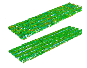
Visualizations such as iso-surface structures can provide a three-dimensional perspective. In figure 21, we compare iso-surface plots of the wall-normal velocity $v$ at $v=-0.02U_0$ obtained from time-window-averaged flow fields at $Re = 4000$, with visualization over the whole computational domain. The average time frame is approximately one turnout time, approximately $U_c T/{L_x \cos \theta }=1$. Five cases include $\theta =0^\circ$, $15^\circ$, $45^\circ$, $60^\circ$ and $75^\circ$. For Couette-type flows of $\theta =0^\circ$ and $\theta =15^\circ$, the signatures of streamwise structures are clearly visible, while for $\theta =45^\circ$, these structures have been greatly attenuated. Cases $\theta =60^\circ$ and $\theta =75^\circ$ show almost no identifiable structure.

Figure 21. Visualization of time-averaged vertical velocity fields $v$ with colouring by spanwise velocity $w$ at $Re=4000$: (a) $\theta = 0^\circ$, (b) $\theta =15^\circ$, (c) $\theta = 45^\circ$, (d) $\theta =60^\circ$, (e) $\theta =75^\circ$.

7.1. Bottom wall $(U^- , d_b^-)$ scaling

For ZSF flows, $u_{\tau,b}=0$, indicating the absence of a local wall-velocity scale. Following Stratford (Reference Stratford1959), Coleman et al. (Reference Coleman, Pirozzoli, Quadrio and Spalart2017) investigated the near-bottom-wall flow at $Re_c$ up to $1.2\times 10^4$ in terms of the alternative, pressure-gradient-based scaling

(7.1a–c)\begin{equation} U^-\equiv \frac{u(d_b)-U_c}{u_p} = f(d_b^-),\quad d_b^-\equiv \frac{d_b\,u_p}{\nu}, \quad u_p \equiv \left(\nu\left|\frac{{\rm d}}{{\rm d} x}\left(\frac{p}{\rho} \right)\right|\right)^{1/3}. \end{equation}

From the integrated skin-friction–pressure-gradient balance for the whole channel, we find that

(7.2a,b)\begin{equation} u_p = \left( \frac{\nu\,u_{\tau,t}^2}{2h} \right)^{1/3},\quad \frac{u_p}{u_{\tau,t}} = \frac{1}{\left(2\,Re_{\tau,t} \right)^{1/3}}. \end{equation}

Using (3.6) with $u_{\tau,b}=0$, neglecting the Reynolds stress term and normalizing using the $(U^{-},d^{-}_b)$ scaling, gives

(7.3)\begin{equation} U^-{=} -\tfrac{1}{2}\left( d^-_b \right)^2. \end{equation}

Figure 22 shows the present DNS/WRLES mean velocity profiles near the bottom wall in $(U^-,d_b^-)$ scaling. The profiles collapse well and agree with (7.3) over almost two decades of $d_b^{-}$. Our WMLES do not provide sufficient near-wall resolution to test this scaling.

Figure 22. Scaled velocity profile near the bottom wall: $U^-$ versus $d^-_b$. Symbols: blue $\triangleleft$, $4000$; black $\triangleright$, $6000$; red $\triangledown$, $10\,000$; blue $\triangle$, $20\,000$. Dash-dotted line indicates $U^- = -(d^-_b)^2/2$.

7.2. Streamwise velocity profiles for ZSF flows

Streamwise velocity profiles are shown in figure 23(a) in top-wall inner scaling units. A logarithmic profile with $U^+ = 1/0.4 \ln y^+ + 5.0$ is also displayed. For our smallest $Re=100$ and $300$, the channel flow is essentially laminar, as shown in the kicked-up profiles at small $d_t^+$. At larger $Re$ up to $Re=10^{10}$ with $Re_{\tau _t} \approx 2.72\times 10^8$, the velocity profiles match the log profile across almost the whole channel height of $2h$. Figure 23(b) shows velocity profiles in outer scaling as $U(y/h)/(U_c$ versus $y/h$, where it is noted that $\theta _c = \theta _c(Re)$ varies with $Re$. Also shown are mean-flow model predictions using PT-II. Model predictions are also shown for $Re = 10^{20}, 10^{50}, 10^{100}$. These show an asymptotic approach to $U/U_0 = \sin \theta$ when $Re \to \infty$ as stated by (4.21a–c). Since, as discussed subsequently, $\theta _c\to 45^\circ$ when $Re\to \infty$, the limit streamwise velocity for ZSF flows is $U(y/h) \to U_c$ except in a thin viscous layer at the top wall. The thickness of this layer as a function of $Re$ can be estimated, an exercise left to the reader. Approach to the limit is extremely slow. Further, for ZSF flows, (2.5) gives $Re_p = Re_{\tau,t}/\sqrt {2}$ so that $Re_p/Re \to 0$ as $Re \to \infty$.

Figure 23. Streamwise velocity profiles of ZSF flows: (a) $U^+$, where the dashed line is the logarithmic line $U^+ =1/0.4 \ln y^+ + 5.0$; (b) model prediction of velocity profiles up to $Re = 10^{100}$, where the dashed line is the model prediction profile for corresponding $Re$. Symbols for $Re$ values: black $\square$, $100$; red $\circ$, $300$; blue $\triangleleft$, $4000$; black $\triangleright$, $6000$; red $\triangledown$, $10\,000$; blue $\triangle$, $20\,000$; red $\blacktriangle$, $10^5$; black $\blacktriangledown$, $10^6$; blue $\blacktriangleleft$, $10^7$; red $\blacktriangleright$, $10^{8}$; black $\scriptstyle \blacksquare$, $10^{9}$; blue $\bullet$, $10^{10}$. Cases with only model prediction: dash-dotted line, $10^{20}$; dash-dot-dotted line, $10^{50}$; solid line, $10^{100}$.

Figure 23(b) also suggests a simple interpretation of the result $\theta _c\to 45^\circ$ when ${Re\to \infty}$ for flows with $Re_{\tau,b} =0$. The limiting plug-flow velocity $U(y) =U_c$ is the only velocity that satisfies both the Dirichlet boundary and also $\textrm {d}U/{\textrm {d} y}=0$ on the bottom plate. Then if $U(y) = U_c$, the volume flow rate is $M = 2 h U_c$. So then $Re_c = U_c h/\nu$ and $Re_M = M/(2\nu ) = U_c h/\nu$. So in the large-$Re$ limit, $Re_c = Re_M$ for ZSF flows, which means $\theta = 45^\circ$.

7.3. Skin friction and mean-flow square velocity

The variation of the critical angle $\theta _c(Re)$ is shown in figure 24(a), where the square symbols are DNS results, the two triangles give WMLES results, and the circles show the six WMLES results. For strictly laminar PCP flow, $\theta _c\approx 18.4^\circ$ (see Appendix A) independent of $Re$. Simulations at $Re=100$ and $300$ show consistency with this value. At $Re=1000$, $\theta _c \approx 33^\circ$, while at $Re=4000$, the bulk flow has transitioned to turbulence with $\theta _c \approx 36^\circ$. As $Re$ increases further, the simulations show a monotonic increase in $\theta _c$. Predictions for the three models CT and PT-I are shown. All models indicate $\theta _c \to 45^\circ$ as $Re\to \infty$, but it is apparent that the limit approach is sub-logarithmic as indicated by (4.10). The top-wall skin-friction variation for ZSF flows is displayed in figure 24(b), where again both laminar and the present model profiles are shown for comparison. The two models agree to plotting accuracy .

Figure 24. Skin-friction property of ZSF flows: (a) critical angle $\theta _c$; (b) skin-friction $Re_{\tau,t}/Re$. Dashotted line indicates laminar exact solution. Turbulent modelling prediction: dash-dot-dotted line, CT model; dashed line, PT-I model. Symbols: red $\scriptstyle \blacksquare$, DNS; black $\blacktriangle$, WRLES; blue $\bullet$, WMLES.

Using the model skin friction law and velocity profile, an estimate of the streamwise mean-flow square velocity can be made. For strict PC flow at $\theta =0^\circ$, the $Re \to \infty$ asymptotic velocity in the bulk flow is $0$ except in thin viscous-dominated layers near the two moving walls. In the frame of reference of the moving bottom wall, the asymptotic mean velocity profile for ZSF flow is $U(y) \to 0$ except in the thin layer near the top wall. Using the model velocity profile (4.18) corrected for the bottom-wall reference frame, and the asymptotic expression (4.9), a scaled mean-flow streamwise square velocity for ZSF flow in the limit $Re\to \infty$ can be obtained as

(7.4)\begin{equation} E = \frac{1}{2h} \int_{{-}h}^{h} \left( \frac{U(y)}{u_{\tau,t}} \right)^2 \,{{\rm d} y} \to \frac{2}{\kappa^2}. \end{equation}

This result states that in the frame of reference of the asymptotic, plug-flow velocity, the streamwise mean-flow square velocity scales on $u_{\tau,t}^2$. This agrees with similar analysis for pure Couette flow.

7.4. Turbulence intensities

For ZSF flows, we expect turbulence intensity profiles to be typical of boundary layer flows except perhaps near the bottom wall, where the flow is laminar over a small region of extent that reduces with respect to the channel width as $Re$ increases. These are shown in figure 25(a) for the four DNS/WRLES values of $Re$. They show an expected inner peak, with its magnitude growing slowly with increasing $Re$, existing at approximately constant $d_t^+ \approx 15$ together with an incipient plateau forming at $Re = 20\,000$. The DNS/WRLES do not reach sufficiently large $Re$ to test the appearance of an outer peak. Intensities for WMLES are displayed together with DNS/WRLES profiles in outer coordinate scaling in figure 25(b). All results show good collapse away from the top wall. Near the bottom wall, all profiles display a steep decrease from approximately $\overline {u'u'}/u_{\tau,t}^2 \sim 1$ to $0$ over the near-wall laminar flow.

Figure 25. Streamwise turbulence intensity profiles for ZSF flows: (a) $\overline {u'u'}/U_{\tau,t}^2$ versus $d_t^+$; (b) $\overline {u'u'}/U_{\tau,t}^2$ versus $(h-y)/h$. Symbols: blue $\blacktriangle$, $Re=4000$; blue $\blacktriangledown$, $Re=6000$; black $\scriptstyle \blacklozenge$, $Re=10\,000$; black ${\bullet }$, $Re=20\,000$. Solid lines: red, $Re=10^5$; black, $Re=10^6$; blue, $Re=10^7$. Dashed lines: red, $Re=10^8$; black, $Re=10^9$; blue, $Re=10^{10}$.