Hostname: page-component-7bb8b95d7b-495rp Total loading time: 0 Render date: 2024-10-01T06:02:24.920Z Has data issue: false hasContentIssue false

The ‘−1’ decay law for some small-scale quantities at large Péclet numbers and fixed Reynolds numbers

Published online by Cambridge University Press:  12 December 2023

S.L. Tang*
Affiliation:
Center for Turbulence Control, Harbin Institute of Technology, Shenzhen, 518055, PR China
R.A. Antonia
Affiliation:
School of Engineering, University of Newcastle, NSW 2308, Australia
L. Djenidi
Affiliation:
Department of Mechanical Engineering, Indian Institute of Technology - Bombay, Powai, Mumbai 400076, India
*
Email address for correspondence: [email protected]

Abstract

The effect of a uniform mean scalar gradient on the small scales of a passive scalar field in statistically stationary homogeneous isotropic turbulence is investigated through the transport equation for the scalar fluctuation. After some manipulation of the equation, it is shown that the effect can be recast in the form $S_\theta ^* {{Pe^{-1}_{\lambda _\theta }}}$ ($S_\theta ^*$ is the non-dimensional scalar gradient, ${{Pe_{\lambda _\theta }}}$ is the turbulent Péclet number). This effect gradually disappears as ${{Pe_{\lambda _\theta }}}$ becomes sufficiently large, implying a gradual approach towards local isotropy of the passive scalar. It is further argued that, for a given $S_\theta ^*$, the normalized odd moments of the scalar derivative tend towards isotropy as 
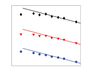
${{Pe^{-1}_{\lambda _\theta }}}$. This is supported by direct numerical simulations data for the normalized odd moments of the scalar derivative at large Péclet numbers. Further, the present derivation leads to the same prediction (${\sim }Sc^{-0.45}$ where Sc is the Schmidt number) as Buaria et al. (Phys. Rev. Lett., vol. 126, no. 3, 2021a, p. 034504) and complements the derivation by the latter authors, which is based on dimensional arguments and the introduction of a new diffusive length scale.

Type
JFM Papers
Copyright
© The Author(s), 2023. Published by Cambridge University Press

1. Introduction

The skewness of the scalar derivative ${S_{3}}$, defined as

(1.1)\begin{equation} {S_{m}} = \frac{{\overline{{{\left( {\dfrac{{\partial {\theta}}}{{\partial {x_1}}}} \right)}^{m}}}}}{{{{\overline{{{\left( {\dfrac{{\partial {\theta}}}{{\partial {x_1}}}} \right)}^2}} }^{m/2}}}}, \quad m=3, \end{equation}

where $\theta$ is the scalar fluctuation and m is a positive integer, is generally of order 1 when the Schmidt number $Sc(\equiv \nu /\kappa$, $\nu$ is the kinematic viscosity and $\kappa$ is the diffusivity of the scalar) is of order 1 in shear flows such as wakes, jets and homogeneous shear flows (e.g. Mestayer et al. Reference Mestayer, Gibson, Coantic and Patel1976; Gibson, Friehe & McConnell Reference Gibson, Friehe and McConnell1977). This has been interpreted as evidence that local isotropy of the passive scalar field is violated (e.g. Mestayer et al. Reference Mestayer, Gibson, Coantic and Patel1976; Sreenivasan & Antonia Reference Sreenivasan and Antonia1977; Sreenivasan, Antonia & Britz Reference Sreenivasan, Antonia and Britz1979; Sreenivasan & Tavoularis Reference Sreenivasan and Tavoularis1980; Subramanian & Antonia Reference Subramanian and Antonia1982; Sreenivasan Reference Sreenivasan1991; Holzer & Siggia Reference Holzer and Siggia1994; Pumir Reference Pumir1994; Tong & Warhaft Reference Tong and Warhaft1994; Sreenivasan & Antonia Reference Sreenivasan and Antonia1997; Shraiman & Siggia Reference Shraiman and Siggia2000; Warhaft Reference Warhaft2000; Yeung, Xu & Sreenivasan Reference Yeung, Xu and Sreenivasan2002; Yeung, Donzis & Sreenivasan Reference Yeung, Donzis and Sreenivasan2005; Monin & Yaglom Reference Monin and Yaglom2007; Yeung & Sreenivasan Reference Yeung and Sreenivasan2014; Clay Reference Clay2017; Sreenivasan Reference Sreenivasan2019; Buaria et al. Reference Buaria, Clay, Sreenivasan and Yeung2021a; Shete et al. Reference Shete, Boucher, Riley and de Bruyn Kops2022). On the other hand, there is evidence that, as $Sc$ increases from approximately $10^{-3}$ to $10^{3}$, $|{S_{3}}|$ along a direction parallel to the mean scalar gradient first increases before decreasing with increasing $Sc$ (e.g. Yeung et al. Reference Yeung, Xu and Sreenivasan2002; Antonia & Orlandi Reference Antonia and Orlandi2003; Brethouwer, Hunt & Nieuwstadt Reference Brethouwer, Hunt and Nieuwstadt2003; Schumacher & Sreenivasan Reference Schumacher and Sreenivasan2003; Yeung et al. Reference Yeung, Xu, Donzis and Sreenivasan2004; Donzis, Sreenivasan & Yeung Reference Donzis, Sreenivasan and Yeung2005; Yasuda et al. Reference Yasuda, Gotoh, Watanabe and Saito2020; Buaria et al. Reference Buaria, Clay, Sreenivasan and Yeung2021a; Shete et al. Reference Shete, Boucher, Riley and de Bruyn Kops2022). In particular, using dimensional arguments, Sreenivasan (Reference Sreenivasan2019), Buaria et al. (Reference Buaria, Clay, Sreenivasan and Yeung2021a) and Shete et al. (Reference Shete, Boucher, Riley and de Bruyn Kops2022) derived relations for $|S_3|$, $|S_5|$ and $|S_7|$. Each of these quantities was found to decrease with $Sc$ as $Sc^{-1/2}$ at a given $Re_\lambda$. However, this behaviour was not supported well by the direct numerical simulations (DNS) data of Buaria et al. (Reference Buaria, Clay, Sreenivasan and Yeung2021a) at $Re_\lambda =140$ over a significant range $Sc (=1\unicode{x2013}512)$. Here, $Re_\lambda$ is the Taylor microscale Reynolds number defined by $\overline {u_1^2}^{1/2}\lambda /\nu$, where $\lambda$ is the longitudinal Taylor microscale defined by $\lambda = \overline {u_1^2}^{1/2}/ \overline {(\partial u_1/\partial x_1)^2}^{1/2}$ and ${ u}_i$ is the fluctuation velocity in the $x_i$ direction. Further, Buaria et al. (Reference Buaria, Clay, Sreenivasan and Yeung2021a) introduced a new diffusive length scale in their dimensional analysis and obtained ${\sim }Sc^{-0.45}$, which is supported reasonably well by their DNS data for $Sc\gtrsim 4$. We recall that Obukhov (Reference Obukhov1949) and Corrsin (Reference Corrsin1951) assumed that the small scales of a passive scalar introduced in a turbulent flow are isotropic in space and stationary in time at sufficiently high Péclet numbers. In this paper, the turbulent Péclet number $Pe_{\lambda _\theta }$ is defined as

(1.2)\begin{equation} Pe_{\lambda_\theta} = \frac{{{{\overline{{u_1^2}} }^{1/2}}{\lambda _\theta }}}{\kappa},\end{equation}

where $\lambda _\theta$ ($\equiv {\overline {{\theta ^2}}^{1/2}}/{\overline {{{(\partial \theta /\partial x_1)}^2}}^{1/2}}$) is the Corrsin microscale. However, it is not clear whether the influence of large-scale forcing, such as that due to the action of the mean scalar gradient on the small-scale anisotropy, is negligible when the Péclet number is not sufficiently large. A knowledge of how and at what rate the small scales of a passive scalar approach isotropy with increasing ${{Pe_{\lambda _\theta }}}$ is of significant importance. For example, local isotropy can significantly simplify the modelling of small scales since one component is generally sufficient to represent all other components. Therefore, the main objective of this paper is to examine how small-scale anisotropy evolves as ${{Pe_{\lambda _\theta }}}$ increases. We first examine how large-scale forcing associated with the mean scalar gradient affects the local anisotropy of the passive scalar and how this anisotropy evolves with ${{Pe_{\lambda _\theta }}}$. Then, the available data for $|{S_{3}}|$, $|{S_{5}}|$ and $|{S_{7}}|$ in the literature are interpreted in the light of the present results. In particular, the relations for $|{S_{3}}|$, $|{S_{5}}|$ and $|{S_{7}}|$, i.e. ${\sim }Sc^{-0.45}$, proposed by Buaria et al. (Reference Buaria, Clay, Sreenivasan and Yeung2021a), will be compared with the present results.

This paper is structured as follows. In § 2, we derive and test the relations between the large-scale forcing associated with the mean scalar gradient and the local anisotropy of the passive scalar. A comparison between the dependence of $|{S_{3}}|$, $|{S_{5}}|$ and $|{S_{7}}|$ on $Sc$, viz. ${\sim }Sc^{-0.45}$ proposed by Buaria et al. (Reference Buaria, Clay, Sreenivasan and Yeung2021a), and the present results is discussed in § 3. Conclusions are given in § 4.

2. Theoretical considerations and discussions

The dynamical equation for the scalar fluctuation $\theta$ is given by Corrsin (Reference Corrsin1952) as

(2.1)\begin{equation} \frac{{\partial \theta }}{{\partial t}} + {\bar{U}_j}\frac{{\partial \theta }}{{\partial {x_j}}} + {u_j}\frac{{\partial \varTheta}}{{\partial {x_j}}} + {u_j}\frac{{\partial \theta }}{{\partial {x_j}}} - \overline{{u_j}\frac{{\partial \theta }}{{\partial {x_j}}}} = \kappa \frac{\partial }{{\partial {x_j}}}\frac{{\partial \theta }}{{\partial {x_j}}}, \end{equation}

where $\varTheta$ is the mean scalar; $\bar {U}_i$ is the mean velocity in the $x_i$ direction. Sreenivasan & Tavoularis (Reference Sreenivasan and Tavoularis1980) derived a transport equation for $\overline {({\partial \theta /\partial {x_1}})^3}$ in a steady, homogeneous shear flow with uniform mean velocity and scalar gradients in the $x_2$ direction (${{\partial \bar {U}_1}}/{{\partial {x_2}}}={\rm const.}$ and ${{\partial \varTheta }}/{{\partial {x_2}}}={\rm const.}$). Using a similar procedure as Sreenivasan & Tavoularis (Reference Sreenivasan and Tavoularis1980), we first differentiate (2.1) with respect to $x_{\alpha }$ (${\alpha }=1,2,3$), then multiply the resulting equation by $({\partial \theta /\partial {x_{\alpha }}})^n$ and finally take the average to obtain

(2.2)\begin{align} &\overline{{{\left( {\frac{{\partial \theta }}{{\partial {x_{\alpha}}}}} \right)}^n}\frac{\partial }{{\partial {x_{\alpha}}}}\frac{{\partial \theta }}{{\partial t}}} + \frac{{\partial {\bar{U}_j}}}{{\partial {x_{\alpha}}}}\overline{{{\left( {\frac{{\partial \theta }}{{\partial {x_{\alpha}}}}} \right)}^n}\frac{{\partial \theta }}{{\partial {x_j}}}} + {\bar{U}_j}\overline{{{\left( {\frac{{\partial \theta }}{{\partial {x_{\alpha}}}}} \right)}^n}\frac{\partial }{{\partial {x_{\alpha}}}}\frac{{\partial \theta }}{{\partial {x_j}}}} \nonumber\\ &\quad +\overline{{{\left( {\frac{{\partial \theta }}{{\partial {x_{\alpha}}}}} \right)}^n}\frac{{\partial {u_j}}}{{\partial {x_{\alpha}}}}} \frac{{\partial \varTheta}}{{\partial {x_j}}} + \overline{{{\left( {\frac{{\partial \theta }}{{\partial {x_{\alpha}}}}} \right)}^n}{u_j}} \frac{\partial }{{\partial {x_{\alpha}}}}\frac{{\partial \varTheta}}{{\partial {x_j}}} + \overline{{{\left( {\frac{{\partial \theta }}{{\partial {x_{\alpha}}}}} \right)}^n}\frac{{\partial {u_j}}}{{\partial {x_{\alpha}}}}\frac{{\partial \theta }}{{\partial {x_j}}}} \nonumber\\ &\quad +\overline{{{\left( {\frac{{\partial \theta }}{{\partial {x_{\alpha}}}}} \right)}^n}{u_j}\frac{\partial }{{\partial {x_{\alpha}}}}\frac{{\partial \theta }}{{\partial {x_j}}}} - \overline{{{\left( {\frac{{\partial \theta }}{{\partial {x_{\alpha}}}}} \right)}^n}} \frac{\partial }{{\partial {x_{\alpha}}}}\overline{{u_j}\frac{{\partial \theta }}{{\partial {x_j}}}} = \kappa \overline{{{\left( {\frac{{\partial \theta }}{{\partial {x_{\alpha}}}}} \right)}^n}\frac{\partial }{{\partial {x_{\alpha}}}}\frac{\partial }{{\partial {x_j}}}\frac{{\partial \theta }}{{\partial {x_j}}}} . \end{align}

Since we consider only the statistically stationary case, we have

(2.3)\begin{equation} \overline{{{\left( {\frac{{\partial \theta }}{{\partial {x_{\alpha}}}}} \right)}^n}\frac{\partial }{{\partial {x_{\alpha}}}}\frac{{\partial \theta }}{{\partial t}}} = \overline{{{\left( {\frac{{\partial \theta }}{{\partial {x_{\alpha}}}}} \right)}^n}\frac{\partial }{{\partial t}}\frac{{\partial \theta }}{{\partial {x_{\alpha}}}}} = \frac{1}{n+1}\frac{\partial }{{\partial t}}\overline{{{\left( {\frac{{\partial \theta }}{{\partial {x_{\alpha}}}}} \right)}^{n+1}}}=0.\end{equation}

In this paper, we focus on the passive scalar field convected by statistically stationary homogeneous isotropic turbulence under a uniform mean scalar gradient in the $x_1$ direction (${{\partial \varTheta }}/{{\partial {x_1}}}$). Therefore, the last two terms on the first line and the second term on the second line of (2.2) can be ignored. Further, since the flow is homogeneous, we have

(2.4)$$\begin{gather} \overline{{{\left( {\frac{{\partial \theta }}{{\partial {x_{\alpha}}}}} \right)}^n}{u_j}\frac{\partial }{{\partial {x_{\alpha}}}}\frac{{\partial \theta }}{{\partial {x_j}}}} = \frac{1}{{n + 1}}\frac{\partial }{{\partial {x_j}}}\overline{{u_j}{{\left( {\frac{{\partial \theta }}{{\partial {x_{\alpha}}}}} \right)}^{n + 1}}} = 0, \end{gather}$$
(2.5)$$\begin{gather}\overline{{{\left( {\frac{{\partial \theta }}{{\partial {x_{\alpha}}}}} \right)}^n}} \frac{\partial }{{\partial {x_{\alpha}}}}\overline{{u_j}\frac{{\partial \theta }}{{\partial {x_j}}}} = \overline{{{\left( {\frac{{\partial \theta }}{{\partial {x_{\alpha}}}}} \right)}^n}} \frac{\partial }{{\partial {x_{\alpha}}}}\frac{{\partial \overline{{u_j}\theta } }}{{\partial {x_j}}} = 0. \end{gather}$$

Finally, (2.2) reduces to

(2.6)\begin{equation} \overline{{{\left( {\frac{{\partial \theta }}{{\partial {x_{\alpha}}}}} \right)}^n}\frac{{\partial {u_1}}}{{\partial {x_{\alpha}}}}} \frac{{\partial \varTheta}}{{\partial {x_1}}} ={-} \overline{{{\left( {\frac{{\partial \theta }}{{\partial {x_{\alpha}}}}} \right)}^n}\frac{{\partial {u_j}}}{{\partial {x_{\alpha}}}}\frac{{\partial \theta }}{{\partial {x_j}}}} + \kappa \overline{{{\left( {\frac{{\partial \theta }}{{\partial {x_{\alpha}}}}} \right)}^n}\frac{\partial }{{\partial {x_{\alpha}}}}\frac{\partial }{{\partial {x_j}}}\frac{{\partial \theta }}{{\partial {x_j}}}} . \end{equation}

The left-hand side term is the (large-scale) mean scalar-gradient production. The two terms on the right side are the small-scale terms, which can be interpreted as representing the production and destruction of $\overline {{{({{{\partial \theta }}/{{\partial {x_{\alpha }}}}} )}^{n + 1}}}$ respectively. Note that, when ${{\partial \varTheta }}/{{\partial {x_1}}}=0$ and $n=1$, (2.6) is the stationary form of the equation for $\overline {{{({{{\partial \theta }}/{{\partial {x_{\alpha }}}}})}^{2}}}$ first written by Corrsin (Reference Corrsin1953). The equation, which contained both mean velocity and mean scalar-gradient terms, was tested by Abe, Antonia & Kawamura (Reference Abe, Antonia and Kawamura2009) in a turbulent channel flow at different Reynolds numbers. Wyngaard (Reference Wyngaard1971) considered (2.6) with $n=1$. He interpreted the first term on the right side of (2.6) as the production rate of $\overline {{{({{{\partial \theta }}/{{\partial {x_{\alpha }}}}})}^{2}}}$ due to the stretching of the temperature field by the turbulent strain field, which is balanced by the molecular smoothing of the gradient temperature field. Since (2.6) contains both large- and small-scale terms, it can be used to quantify the effect of the large-scale forcing associated with the mean scalar gradient on small-scale quantities. When $n$ is even and ${\alpha }=2$ or 3, the first term in (2.6) is zero if local isotropy is satisfied since all combinations of the indices in $\overline {{{({{{\partial \theta }}/{{\partial {x_{\alpha }}}}})}^n}({{\partial {u_1}}}/{{\partial {x_{\alpha }}}})}$ will lead to the Kronecker delta $\delta _{1{\alpha }}$ (${\alpha }=2$ or 3) under the assumption of local isotropy. As an example, the first term in (2.6) for ${\alpha }=2$ and $n=2$ can be written as

(2.7)\begin{equation} \overline{\frac{{\partial {u_1}}}{{\partial {x_2}}}\frac{{\partial \theta }}{{\partial {x_2}}}\frac{{\partial \theta }}{{\partial {x_2}}}} \frac{{\partial \varTheta }}{{\partial {x_1}}} = \frac{3}{4}\left( {{\delta _{12}}{\delta _{22}} + {\delta _{12}}{\delta _{22}} - \frac{2}{3}{\delta _{12}}{\delta _{22}}} \right)\overline{\frac{{\partial {u_1}}}{{\partial {x_1}}}{{\left( {\frac{{\partial \theta }}{{\partial {x_1}}}} \right)}^2}} \frac{{\partial \varTheta }}{{\partial {x_1}}} = 0, \end{equation}

after using the isotropic form of a single-point fourth-order velocity derivative tensor $\overline {({{\partial {u_i}}}/{{\partial {x_j}}})({{\partial \theta }}/{{\partial {x_n}}})({{\partial \theta }}/{{\partial {x_m}}})}$ (e.g. Antonia & Browne Reference Antonia and Browne1983; Wyngaard Reference Wyngaard2010). When $n$ is odd and ${\alpha }=2$ or 3, the first term in (2.6) is also zero if local isotropy is satisfied since all combinations of the indices in $\overline {{{( {{{\partial \theta }}/{{\partial {x_{\alpha }}}}})}^n}({{\partial {u_1}}}/{{\partial {x_{\alpha }}}})}$ will lead to the Kronecker delta $\delta _{1{\alpha }}$ (${\alpha }=2$ or 3) or the permutation symbol $\epsilon _{1{\alpha \alpha }}$ or $\epsilon _{{\alpha \alpha \alpha }}$ under the assumption of local isotropy. Therefore, in (2.6), we only consider the subscript ${\alpha }=1$, which represents the direction of the mean scalar gradient. After normalization by ${\overline {{{({\partial \theta /\partial {x_1}})}^2}} ^{(n + 1)/2}}{\overline {{{({\partial {u_1}/\partial {x_1}})}^2}} ^{1/2}}$, the first term in (2.6) becomes

(2.8) \begin{equation} \left.\begin{array}{c@{}} \dfrac{{\overline{{{\left( {\dfrac{{\partial \theta }}{{\partial {x_1}}}} \right)}^n}\dfrac{{\partial {u_1}}}{{\partial {x_1}}}} \dfrac{{\partial \varTheta }}{{\partial {x_1}}}}}{{{{\overline{{{( {\partial \theta /\partial {x_1}} )}^2}} }^{(n + 1)/2}}{{\overline{{{( {\partial {u_1}/\partial {x_1}} )}^2}} }^{1/2}}}} = \dfrac{{\overline{{{\left( {\dfrac{{\partial \theta }}{{\partial {x_1}}}} \right)}^n}\dfrac{{\partial {u_1}}}{{\partial {x_1}}}} \dfrac{{\partial \varTheta }}{{\partial {x_1}}}}}{{{{\overline{{{( {\partial \theta /\partial {x_1}} )}^2}} }^{n/2}}{{\overline{{{( {\partial {u_1}/\partial {x_1}} )}^2}} }^{1/2}}{{\overline{{{( {\partial \theta /\partial {x_1}} )}^2}} }^{1/2}}}}\\ \dfrac{{{R_n}\dfrac{{\partial \varTheta }}{{\partial {x_1}}}}}{{{{\overline{{{( {\partial \theta /\partial {x_1}} )}^2}} }^{1/2}}}} = \dfrac{{{R_n}6\kappa {{\overline{{\theta ^2}} }^{1/2}}{{\overline{u_1^2} }^{1/2}}\dfrac{{\partial \varTheta }}{{\partial {x_1}}}{{\overline{{{\left( {\dfrac{{\partial \theta }}{{\partial {x_1}}}} \right)}^2}} }^{1/2}}}}{{{{\overline{{\theta ^2}} }^{1/2}}{{\overline{u_1^2} }^{1/2}}6\kappa \overline{{{( {\partial \theta /\partial {x_1}} )}^2}}}} = \dfrac{{6{R_n}S_\theta ^*}}{{Pe_{{\lambda_\theta}}}} \end{array} \right\},\end{equation}

where $Pe_{{\lambda _\theta }}$ is defined in (1.2); $S_\theta ^*$ is defined as

(2.9)\begin{equation} S_\theta^* = \frac{{{{\overline{{\theta ^2}}}^{1/2}}{{\overline{u_1^2} }^{1/2}}\dfrac{{\partial \varTheta }}{{\partial {x_1}}}}}{{{{\bar \varepsilon }_\theta }}}, \end{equation}

with ${{\bar {\varepsilon }_\theta } = 6\kappa \overline {{{({{{\partial \theta }}/{{\partial {x_1}}}})}^2}}}$; for convenience, we refer to $S_\theta ^*$ as the non-dimensional scalar gradient. Here, ${R_n}$ is the normalized correlation involving the streamwise derivative of $\theta$ and $u_1$, defined as

(2.10)\begin{equation} {R_n} = \frac{{\overline{{{\left( {\dfrac{{\partial \theta }}{{\partial {x_1}}}} \right)}^n}\dfrac{{\partial {u_1}}}{{\partial {x_1}}}} }}{{{{\overline{{{({\partial \theta /\partial {x_1}} )}^2}} }^{n/2}}{{\overline{{{({\partial {u_1}/\partial {x_1}})}^2}} }^{1/2}}}}. \end{equation}

Finally, after normalization by ${\overline {{{( {\partial \theta /\partial {x_1}} )}^2}} ^{(n + 1)/2}}{\overline {{{({\partial {u_1}/\partial {x_1}} )}^2}} ^{1/2}}$, (2.6) for ${\alpha }=1$ can be rewritten as

(2.11)\begin{equation} \frac{{6{R_n}S_\theta ^*}}{{Pe_{\lambda_\theta} }} = {A_{n}},\end{equation}

where $A_{n}$ is defined as

(2.12)\begin{align} {A_n} = \frac{{ - \overline{{{\left( {\dfrac{{\partial \theta }}{{\partial {x_1}}}} \right)}^n}\dfrac{{\partial {u_j}}}{{\partial {x_1}}}\dfrac{{\partial \theta }}{{\partial {x_j}}}} + \kappa \overline{{{\left( {\dfrac{{\partial \theta }}{{\partial {x_1}}}} \right)}^n}\dfrac{\partial}{{\partial {x_1}}}\dfrac{\partial }{{\partial {x_j}}}\dfrac{{\partial \theta }}{{\partial {x_j}}}}}}{{{{\overline{{{({\partial \theta /\partial {x_1}} )}^2}} }^{(n + 1)/2}}{{\overline{{{({\partial {u_1}/\partial {x_1}})}^2}} }^{1/2}}}}. \end{align}

The numerator of $A_n$ is simply the right-hand side of (2.6) with $\alpha =1$. In that respect, $A_n$ represents the normalized sum of the production and destruction of $\overline {{{( {{{\partial \theta }}/{{\partial {x_{1}}}}} )}^{n + 1}}}$. Some remarks are warranted on the use of $\overline {{{( {{{\partial \theta }}/{{\partial {x_1}}}} )}^2}}$, which is one of the three components in the full scalar dissipation rate defined as $2 \kappa \overline {{{( {{{\partial \theta }}/{{\partial {x_i}}}} )}^2}}$, in equations (2.11) and (2.9). The values of $\overline {{{( {{{\partial \theta }}/{{\partial {x_i}}}} )}^2}}$ along the directions perpendicular to the mean scalar gradient, i.e. the $x_2$ and $x_3$ directions, should be equal because of the symmetry. On the other hand, Yeung et al. (Reference Yeung, Xu and Sreenivasan2002) showed that the ratio of parallel-to-perpendicular scalar-gradient variances (i.e. $\overline {{{({\partial \theta /\partial {x_1}})}^2}} /\overline {{{({\partial \theta /\partial {x_2}})}^2}}$ and $\overline {{{( {\partial \theta /\partial {x_1}} )}^2}} /\overline {{{({\partial \theta /\partial {x_3}})}^2}}$) is close to unity (their table III or figure 11a). In particular, this ratio is equal to 1.05 at $Sc=1$ and $Re_\lambda =140$ and 240, respectively (their table III). This implies that local isotropy is satisfied adequately in the context of the ratio of parallel-to-perpendicular scalar-gradient variances in this flow and justifies the use of $\overline {{{( {{{\partial \theta }}/{{\partial {x_1}}}} )}^2}}$ in (2.11) and (2.9). It is worth mentioning that local isotropy does not require ${R_2}$, ${R_4}$ and ${R_6}$ in (2.11) to be zero. For example, ${R_2}$, the mixed velocity-scalar derivative skewness, represents the production of ${\bar {\varepsilon }_\theta }$ generated by stretching of the scalar field as a result of the turbulent strain rate. Further, for $n=2,4,6$ and when local isotropy is satisfied, any combination of the indices in ${A_2}, {A_4}$ and ${A_6}$ will lead to a term involving the permutation symbols $\epsilon _{111}$, $\epsilon _{11j}$ or $\epsilon _{1jj}$, which are zero. Based on the above analysis, it can be concluded from (2.11) that, due to the presence of the mean shear, ${A_2}, {A_4}$ and ${A_6}$ may not be 0 at finite $Pe_{\lambda _\theta }$ and thus the flow is anisotropic in the context of ${A_2}, {A_4}$ and ${A_6}$. Therefore, (2.11) provides a relation between the mean scalar gradient and the local anisotropy. Namely, since, regardless of whether local isotropy is satisfied, the large-scale production term (the term on left-hand side of (2.11)) is non-zero and the corresponding small-scale terms (${A_2}, {A_4}$ and ${A_6}$ in (2.11)) are zero when local isotropy is assumed, we can use (2.11) to quantify the effect of the large-scale forcing caused by the mean shear on the degree of isotropy of the small scales. Specifically, the relation shows how the level of local anisotropy depends on the magnitudes of ${S^*_\theta }$, $Pe_{\lambda _\theta }$ and ${R_n}$ for $n=2,4$ and 6. If ${R_n}{S^*_\theta }$ for $n=2,4, 6$ does not increase as rapidly as $Pe_{\lambda _\theta }$, ${A_2}, {A_4}$ and ${A_6}$ should then go to zero when $Pe_{\lambda _\theta }$ is sufficiently large, irrespective of the magnitude of ${S^*_\theta }$. In particular, for a given ${S^*_\theta }$, if ${R_n}$ for $n=2,4,6$ are constant, $A_n$ will behave as $Pe_{\lambda _\theta }^{-1}$ in statistically stationary homogeneous isotropic turbulence with a uniform mean scalar gradient. Figure 1(a) shows the distributions of $S^*_\theta$ and $R_2$ in statistically stationary homogeneous isotropic turbulence with a uniform mean scalar gradient at $Re_\lambda =38$. We can observe that the magnitude of $R_2$ decreases slightly as $Sc$ increases for $Sc\lesssim 10$ and appears to be approximately constant for $Sc\gtrsim 10$. Similarly, the magnitude of $S^*_\theta$ increases as $Sc$ increases for $Sc\lesssim 10$ and also becomes approximately constant for $Sc\gtrsim 10$. We thus can conclude that $A_2$ should behave as $Pe_{\lambda _\theta }^{-1}$ for $Sc\gtrsim 10$. It is worth mentioning that the values of $R_4$ and $R_6$ in this flow are not available. However, $R_2$, $R_4$ and $R_6$ can be related to the normalized high-order moments of scalar derivatives via the following Cauchy–Schwarz inequalities:

(2.13a)$$\begin{gather} \overline{\left| {{{\left( {\frac{{\partial \theta }}{{\partial {x_1}}}} \right)}^2}\frac{{\partial {u_1}}}{{\partial {x_1}}}} \right|} \le {\overline{{{\left( {\frac{{\partial \theta }}{{\partial {x_1}}}} \right)}^4}} ^{1/2}}{\overline{{{\left( {\frac{{\partial {u_1}}}{{\partial {x_1}}}} \right)}^2}} ^{1/2}} \Rightarrow | {{R_2}} | \le \frac{{{{\overline{{{( {\partial \theta /\partial {x_1}} )}^4}} }^{1/2}}}}{{\overline{{{( {\partial \theta /\partial {x_1}} )}^2}} }} = F_{{\parallel} 4}^{1/2}, \end{gather}$$
(2.13b)$$\begin{gather}\overline{\left| {{{\left( {\frac{{\partial \theta }}{{\partial {x_1}}}} \right)}^4}} \right|\frac{{\partial {u_1}}}{{\partial {x_1}}}} \le {\overline{{{\left( {\frac{{\partial \theta }}{{\partial {x_1}}}} \right)}^8}} ^{1/2}}{\overline{{{\left( {\frac{{\partial {u_1}}}{{\partial {x_1}}}} \right)}^2}} ^{1/2}} \Rightarrow | {{R_4}} | \le \frac{{{{\overline{{{( {\partial \theta /\partial {x_1}} )}^8}} }^{1/2}}}}{{{{\overline{{{( {\partial \theta /\partial {x_1}} )}^2}} }^2}}} = F_{{\parallel} 8}^{1/2}, \end{gather}$$
(2.13c)$$\begin{gather}\overline{\left| {{{\left( {\frac{{\partial \theta }}{{\partial {x_1}}}} \right)}^6}\frac{{\partial {u_1}}}{{\partial {x_1}}}} \right|} \le {\overline{{{\left( {\frac{{\partial \theta }}{{\partial {x_1}}}} \right)}^{12}}} ^{1/2}}{\overline{{{\left( {\frac{{\partial {u_1}}}{{\partial {x_1}}}} \right)}^2}} ^{1/2}} \Rightarrow | {{R_6}} | \le \frac{{{{\overline{{{( {\partial \theta /\partial {x_1}} )}^{12}}} }^{1/2}}}}{{{{\overline{{{( {\partial \theta /\partial {x_1}} )}^2}} }^3}}} = F_{{\parallel} 12}^{1/2}, \end{gather}$$

where $F_{\parallel 4}$, $F_{\parallel 8}$ and $F_{\parallel 12}$ are the normalized 4th, 8th and 12th moments of scalar derivatives along the direction parallel to the mean gradient. The inequalities in (2.13) imply that the magnitudes of $R_2$, $R_4$ and $R_6$ should not exceed those of $F_{\parallel 4}$, $F_{\parallel 8}$ and $F_{\parallel 12}$. Figure 11(c) of Yeung et al. (Reference Yeung, Xu and Sreenivasan2002) ($Sc=0.25\unicode{x2013} 64$) shows that the flatness of scalar derivatives along directions parallel ($F_{\parallel 4}$) and perpendicular ($F_{ \bot 4}$) to the mean gradient are approximately constant for $Sc>10$ at $Re_\lambda =38$. Also, at a higher $Re_\lambda (=140)$, figure 8 of Buaria et al. (Reference Buaria, Clay, Sreenivasan and Yeung2021a) ($Sc=1\unicode{x2013} 512$) shows that the normalized $4$th, $6$th and $8$th moments of scalar derivatives along directions parallel ($F_{\parallel 4}$, $F_{\parallel 6}$ and $F_{\parallel 8}$) and perpendicular ($F_{\bot 4}$, $F_{\bot 6}$ and $F_{\bot 8}$) to the mean gradient approach each other and become independent of $Sc$ for $Sc\gtrsim 8$. Based on this information, for the normalized moments of the scalar derivatives and the inequalities in (2.13), it seems reasonable to assume that $R_4$ and $R_6$ become independent of $Sc$, like $R_2$ (figure 1a), for $Sc>10$. In this situation, we can conclude that $A_4$ and $A_6$, like $A_2$, should behave as $Pe_{\lambda _\theta }^{-1}$ for $Sc\gtrsim 10$.

Figure 1. (a) Dependence of ${S^*_\theta }$ (${\bigtriangledown}$, blue) and $R_2$ ($\bullet$, red) on $Sc$ for $Re_\lambda =38$. (b) Dependence of $|S_3|$ ($\bullet$, blue), $|S_5|$ ($\blacktriangledown$, red) and $|S_7|$ (${\blacklozenge}$) at $Re_\lambda =38$. Lines: ${\sim }Pe_{{\lambda _\theta }}^{-1}$. The horizontal arrows in (a) and (b) indicate the region in which $R_2\approx const$ and ${S^*_\theta }\approx const$. To plot (a) and (b), we have used the DNS data of Yeung et al. (Reference Yeung, Xu and Sreenivasan2002); see text for details.

We recall that $|{S_{3}}|$, $|{S_{5}}|$ and $|{S_{7}}|$ are frequently used to test local isotropy of a passive scalar. In this context, it is interesting to examine whether $|{S_{3}}|$, $|{S_{5}}|$ and $|{S_{7}}|$ will follow the prediction (2.11), equivalently whether $|{S_{3}}|$, $|{S_{5}}|$ and $|{S_{7}}|$ will follow ${A_n}\sim Pe_{\lambda _\theta }^{-1}$ for $n=2,4,6$ for $Sc\gtrsim 10$. Although ${A_n}$ and $|{S_m}|$ are different small-scale quantities, they have some features in common. For example, they both are strongly affected by the uniform mean scalar gradient; they both quantify the degree of local anisotropy of the passive scalar. Figure 1(b) shows the distributions of $|{S_{3}}|$, $|{S_{5}}|$ and $|{S_{7}}|$ vs $Pe_{\lambda _\theta }$, using the data of Yeung et al. (Reference Yeung, Xu and Sreenivasan2002). In order to obtain the values of $Pe_{\lambda _\theta }$, we have used the following relation:

(2.14)\begin{equation} \frac{{P{e_{{\lambda _\theta }}}}}{{R{e_\lambda }}} = {\left( {\frac{{6Sc{R_\theta }}}{5}} \right)^{1/2}} ,\end{equation}

where the time scale ratio $R_\theta$ can be rewritten as

(2.15)\begin{equation} {R_\theta } = \frac{{\overline{{\theta ^2}} /{{\bar \varepsilon }_\theta }}}{{\overline{{q^2}} /\bar \varepsilon }} = \frac{{\overline{{\theta ^2}} \bar \varepsilon }}{{3\overline{u_1^2} {{\bar \varepsilon }_\theta }}} = \frac{{\dfrac{{\bar \varepsilon L}}{{{{\overline{u_1^2} }^{3/2}}}}}}{{\dfrac{{3{{\bar \varepsilon }_\theta }L}}{{{{\overline{u_1^2} }^{1/2}}\overline{{\theta ^2}} }}}} = \frac{{{C_\varepsilon }}}{{3{C_{\varepsilon \theta }}}}, \end{equation}

where $L$ is the integral length scale. The parameters $C_\varepsilon$ and $C_{\varepsilon \theta }$ at $Re_\lambda$=38 and $Sc=0.25\unicode{x2013} 64$ are calculated from table 1 of Donzis et al. (Reference Donzis, Sreenivasan and Yeung2005). Note that, at $Pe_{\lambda _\theta }=121$ (or equivalently $Sc=16$), there are two values of $|S_m|$ at each $m$ (=3,5,7) (see figure 12 of Yeung et al. Reference Yeung, Xu and Sreenivasan2002), corresponding to two simulations at different spatial resolutions, i.e. $k_{max}\eta _ B=1.48$ and 2.95 (see table I of Yeung et al. (Reference Yeung, Xu and Sreenivasan2002); here, $k_{max}$ is the resolved highest wavenumber and $\eta _ B$ is the Batchelor length scale). In figure 1(b), the values of $|S_m|$ at $k_{max}\eta _ B=1.48$ are not shown since small values of $k_{max}\eta _ B$ would result in an underestimation of the magnitude of $|S_m|$; for example, this can be observed from table III of Yeung et al. (Reference Yeung, Xu and Sreenivasan2002) in the context of $|S_3|$ and $|S_4|$ at $Sc=16$. We can observe from figure 1(b) that $|S_3|$, $|S_5|$ and $|S_7|$ exhibit a tendency to behave as $Pe_{\lambda _\theta }^{-1}$ for $Sc>10$ (or equivalently ${Pe_{{\lambda _\theta }}}>91$). Namely, the flow approaches local isotropy as $Pe_{\lambda _\theta }^{-1}$ in the context of $|S_3|$, $|S_5|$ and $|S_7|$.

We now examine whether the behaviours of $|S_3|$, $|S_5|$ and $|S_7|$ follow the behaviours of ${A_2}, {A_4}$ and ${A_6}$ (or the prediction (2.11)) at $Re_\lambda =140$. Buaria et al. (Reference Buaria, Clay, Sreenivasan and Yeung2021b) show that $C_{\varepsilon \theta }$ decreases as $Sc$ increases from 1 to 512 at $Re_\lambda =140$ (see their figure 2, which was digitized to replot $|S_3|$, $|S_5|$ and $|S_7|$ vs $Pe_{\lambda _\theta }$). Figure 2 shows the distributions of $|S_3|$, $|S_5|$ and $|S_7|$ of Buaria et al. (Reference Buaria, Clay, Sreenivasan and Yeung2021a) as a function of $Pe_{\lambda _\theta }$. To replot the data we used (2.14) and (2.15) with $C_\varepsilon =0.46$ (estimated using data in table 1 of Donzis et al. (Reference Donzis, Sreenivasan and Yeung2005) at $Re_\lambda =140$) and the values of $C_{\varepsilon \theta }$, the distributions of $|S_3|$, $|S_5|$ and $|S_7|$ vs $Sc$ for the data of Buaria et al. (Reference Buaria, Clay, Sreenivasan and Yeung2021a) are replotted in figure 2 as a function of $Pe_{\lambda _\theta }$. Figure 2 shows that $|S_3|$, $|S_5|$ and $|S_7|$ follow approximately the behaviour $Pe_{\lambda _\theta }^{-1}$ for $Sc>10$ (or equivalently ${P{e_{{\lambda _\theta }}}}>257$). Namely, the flow approaches local isotropy as $Pe_{\lambda _\theta }^{-1}$ in the context of $|S_3|$, $|S_5|$ and $|S_7|$. We can observe that the behaviour of $|S_3|$, $|S_5|$ and $|S_7|$ for $Sc>10$ in figures 1(b) and 2 is consistent with the prediction in (2.11).

Figure 2. Dependence of $|S_3|$ ($\bullet$, blue), $|S_5|$ ($\blacktriangledown$, red) and $|S_7|$ (${\blacklozenge}$) on $Pe_{\lambda _\theta }$ for $Re_\lambda =140$. Lines: ${\sim }{P{e_{{\lambda _\theta }}}}^{-1}$. The horizontal arrow indicates the region where $Sc>10$, $S_\theta ^*$ and $|R_2|$ are approximately constant and the normalized $4$th, $6$th and $8$th moments of scalar derivatives along directions parallel and perpendicular to the mean gradient are also approximately constant. The symbols correspond to the DNS data of Buaria et al. (Reference Buaria, Clay, Sreenivasan and Yeung2021a).

3. Discussion

Using dimensional analysis, Sreenivasan (Reference Sreenivasan2019), Buaria et al. (Reference Buaria, Clay, Sreenivasan and Yeung2021a) and Shete et al. (Reference Shete, Boucher, Riley and de Bruyn Kops2022) have derived relations for $|S_3|$, $|S_5|$ and $|S_7|$, i.e.

(3.1)\begin{equation} |{S_m}| \sim Sc^{ - 1/2},\end{equation}

($m=3,5,7$) at a given $Re_\lambda$. On the other hand, using (2.14) and (2.15), (2.11) can be rewritten as

(3.2)\begin{equation} {A_n} = \sqrt {90} \frac{{{R_n}S_\theta ^*}}{{R{e_\lambda }}}{\left( {\frac{{{C_{\varepsilon \theta }}}}{{Sc{C_\varepsilon }}}} \right)^{1/2}}. \end{equation}

We recall $|{S_m}| \sim {A_n}$ for $Sc>10$ (figures 1b and 2). Equation (3.2) can be reduced to (3.1), provided $R_n$, $S_\theta ^*$ and $C_{\varepsilon \theta }$ do not depend on $Sc$ at a given $Re_\lambda$. As shown in figure 1(a), $R_2$ and $S_\theta ^*$ are approximately constant for $Sc>10$. However, the available data indicate that $C_{\varepsilon \theta }$ decreases as $Sc$ increases at a given $Re_\lambda$ (Buaria, Yeung & Sawford Reference Buaria, Yeung and Sawford2016; Buaria et al. Reference Buaria, Clay, Sreenivasan and Yeung2021b). In particular, Buaria et al. (Reference Buaria, Clay, Sreenivasan and Yeung2021b) showed that there is an empirical relation for $C_{\varepsilon \theta }$ vs $Sc$, i.e. $C_{\varepsilon \theta }=1/ \log Sc$. They further showed that the $1/ \log Sc$ dependence can be replaced by a weak power-law relation, i.e. $\sim Sc^{-0.1}$ (Buaria et al. Reference Buaria, Clay, Sreenivasan and Yeung2021a). After introducing a new diffusive length scale in their dimensional analysis, they obtained

(3.3)\begin{equation} |{S_m}| \sim Sc^{ - 0.45}.\end{equation}

However, substituting $C_{\varepsilon \theta } \sim Sc^{-0.1}$ into (3.2), we obtain

(3.4)\begin{equation} {A_n} \sim Sc^{ - 0.55},\end{equation}

which should be tenable for $Sc>10$. We now plot $|{S_m}|$ ($m=3, 5, 7$) vs $Sc$ using the data of Buaria et al. (Reference Buaria, Clay, Sreenivasan and Yeung2021a) in figure 3. Also shown are the predictions of (3.3) and (3.4), i.e. ${\sim }Sc^{ - 0.45}$ and ${\sim }Sc^{ - 0.55}$. Overall, (3.3) seems to be superior to (3.4) when the three data points for $Sc<10$ are included. However, since (3.4) only applies to the range $Sc>10$, we can conclude that both (3.3) and (3.4) provide similarly adequate descriptions of the data when $Sc>10$.

Figure 3. Dependence of $|S_3|$ ($\bullet$, blue), $|S_5|$ ($\blacktriangledown$, red) and $|S_7|$ (${\blacklozenge}$) on $Sc$ at $Re_\lambda =140$. Solid Lines: ${\sim }Sc^{-0.55}$, i.e. the prediction of (3.4). Dash-dotted lines: ${\sim }Sc^{-0.45}$, i.e. the prediction of (3.3). The horizontal arrow indicates the region where $Sc>10$, $S_\theta ^*$ and $|R_2|$ are approximately constant and the normalized $4$th, $6$th and $8$th moments of scalar derivatives along directions parallel and perpendicular to the mean gradient are also approximately constant. The symbols correspond to the DNS data of Buaria et al. (Reference Buaria, Clay, Sreenivasan and Yeung2021a).

It is of interest to explain the difference between the predictions of (3.3) and (3.4), i.e. ${\sim }Sc^{ - 0.45}$ and ${\sim }Sc^{ - 0.55}$ for $Sc<10$. We can observe from figure 1(a) that the variation of $|R_2|$ in the range $Sc=1\unicode{x2013} 10$ is actually very small. However, the magnitude of $S_\theta ^*$ increases from 1.78 to 2.22 when $Sc$ increases from 1 to 8 at $Re_\lambda =38$ (figure 1a); the magnitude of $S_\theta ^*$ appears to be independent of $Re_\lambda$, at least for $Sc=1$ (figure 4a). In order to take into account the impact of the variation of $S_\theta ^*$ at low $Sc$ on (3.2), a power-law fit is used to the data of $S_\theta ^*$ at $Re_\lambda =38$, 140 and 240. This fit is $S_\theta ^*=1.79Sc^{{0.1}}$ (figure 4a). Note that, here, we are mainly interested in the range $Sc=1\unicode{x2013} 10$. As discussed in the context of figure 1(a), $S_\theta ^*$ is approximately constant for $Sc=10\unicode{x2013} 64$ (see also the blue symbols in figure 4a). Substituting $C_{\varepsilon \theta } \sim Sc^{-0.1}$ (see the discussion in the context of (3.3) or Buaria et al. Reference Buaria, Clay, Sreenivasan and Yeung2021a) and $S_\theta ^*=1.79Sc^{{0.1}}$ in (3.2), we obtain

(3.5)\begin{equation} {A_n} \sim Sc^{ - 0.4{{5}}},\end{equation}

which is exactly the same as the prediction of (3.3), i.e. ${\sim }Sc^{ - 0.45}$ proposed by Buaria et al. (Reference Buaria, Clay, Sreenivasan and Yeung2021a). A possible reason why the approach of Buaria et al. (Reference Buaria, Clay, Sreenivasan and Yeung2021a) and the present approach lead to the same prediction may be as follows. One of the key ingredients of the present approach is the use of the turbulent Péclet number $Pe_{\lambda _\theta }$, defined in (1.2), which can be written as a function of $Re_\lambda$, $Sc$, $C_\varepsilon$ and $C_{\varepsilon \theta }$ (see (2.14) and (2.15)). Combining (1.2), (2.14) and (2.15), we can obtain

(3.6)\begin{equation} Pe_{\lambda_\theta} = \frac{{{{\overline{{u_1^2}} }^{1/2}}{\lambda _\theta }}}{\kappa }= \frac{{{{\overline{{u_1^2}} }^{1/2}}\lambda \nu{\lambda _\theta }}}{\kappa \nu \lambda}=R{e_\lambda }Sc\frac{\lambda _\theta}{\lambda} =R{e_\lambda }{\left( {\frac{{6Sc{R_\theta }}}{5}} \right)^{1/2}} =R{e_\lambda }{\left( {\frac{{2Sc{C_\varepsilon }}}{5C_{\varepsilon \theta }}} \right)^{1/2}}, \end{equation}

which leads to

(3.7)\begin{align} \frac{\lambda _\theta}{\lambda} ={\left( {\frac{{2{C_\varepsilon }}}{5ScC_{\varepsilon \theta }}} \right)^{1/2}}\approx {\left( {\frac{{2{C_\varepsilon }}}{5Sc0.69Sc^{{-}0.1}}} \right)^{1/2}}= {\left( {\frac{{2{C_\varepsilon }}}{3.45}} \right)^{1/2}} Sc^{{-}0.45}=0.52 Sc^{{-}0.45}.\end{align}

The relations $C_{\varepsilon \theta }\approx 0.69Sc^{-0.1}$ (estimated from figure 2 of Buaria et al. Reference Buaria, Clay, Sreenivasan and Yeung2021b) and $C_\varepsilon =0.475$ (Yeung & Zhou Reference Yeung and Zhou1997) at $Re_\lambda =140$ have been used in (3.7). Equation (3.7) indicates that ${\lambda _\theta }/{\lambda }$ should decrease as $Sc$ increases. Further, substituting (3.7) into the fourth term of (3.6) leads to $Pe_{\lambda _\theta } \approx 0.52 R{e_\lambda }Sc^{0.55}$. Evidently, $Pe_{\lambda _\theta }$ is a function of $R{e_\lambda }$ and $Sc$; a large $Pe_{\lambda _\theta }$ can be obtained either by increasing $Sc$ at a fixed $R{e_\lambda }$ or by increasing $R{e_\lambda }$ at a fixed $Sc$. The isotropic relation between $\lambda$ and $\eta$ is $\lambda /\eta =15^{1/4}Re_\lambda ^{1/2}$. Using this relation, (3.7) can be further written as

(3.8)\begin{equation} \lambda _\theta \approx 0.52 Sc^{{-}0.45} \lambda =Sc^{{-}0.45}Re_\lambda^{1/2}\eta.\end{equation}

On the other hand, the key ingredient in Buaria et al. (Reference Buaria, Clay, Sreenivasan and Yeung2021a) is the introduction of a new diffusive length scale, i.e. $\eta _D=\eta Sc^{-0.45}$ (see their (4)). Therefore, $\lambda _\theta =\eta _D$ only when $Re_\lambda =1$. However, it is interesting to note ${\lambda _\theta }\sim \eta _D$ at any given $Re_\lambda$; this is a possible reason why both Buaria et al. (Reference Buaria, Clay, Sreenivasan and Yeung2021a) and the present approach lead to the same prediction.

Figure 4. (a) Dependence of ${S^*_\theta }$ on $Sc$ at $Re_\lambda =38$ ($\bigtriangledown$, blue), 140 (${\blacksquare}$) and 240 ($\circ$, red). Solid line: $1.79 Sc^{{0.1}}$. The symbols correspond to the DNS data of Yeung et al. (Reference Yeung, Xu and Sreenivasan2002). (b) Dependence of $|S_3|$ ($\bullet$, blue), $|S_5|$ ($\blacktriangledown$, red) and $|S_7|$ (${\blacklozenge}$) on $Sc$ at $Re_\lambda =140$. Solid lines: ${\sim }Sc^{-0.4{{5}}}$, i.e. the prediction of (3.5). The symbols correspond to the DNS data of Buaria et al. (Reference Buaria, Clay, Sreenivasan and Yeung2021a).

We conclude this section by examining the data of Shete et al. (Reference Shete, Boucher, Riley and de Bruyn Kops2022) at much higher $Re_\lambda (=633)$ and $Sc=0.1$, 0.7, 1 and 7. Since the maximum value of $Sc (=7)$ is relatively low, we here only test the prediction of (3.5) which includes the variation of $S_\theta ^*$ at low $Sc$. It can be observed from figure 5(a) that (3.5) is satisfied approximately for $Sc\gtrsim 0.7$. As was discussed in the context of figure 4(b), the prediction of (3.3) is the same as that of (3.5). It is worth mentioning that Buaria & Sreenivasan (Reference Buaria and Sreenivasan2023) further examined the prediction of (3.3) in the context of $|S_3|$, i.e. $|S_3|\sim Sc^{ - 0.45}$, at $Re_\lambda =140$, 390 and 633 and found that $|S_3|\sim Sc^{ - 0.45}$ is satisfied approximately for $Sc\gtrsim 3$ at all $Re_\lambda$ (see their figure 1). Further, substituting $S_\theta ^*=1.79Sc^{{0.1}}$ into (2.11) leads to

(3.9)\begin{equation} {A_n} = \frac{{6{R_n}S_\theta ^*}}{{P{e_{{\lambda _\theta }}}}} = \frac{{6{R_n}1.79S{c^{0.1}}}}{{P{e_{{\lambda _\theta }}}}} \approx \frac{{6{R_n}1.79}}{{P{e_{{\lambda _\theta }}}}}{\left( {\frac{{P{e_{{\lambda _\theta }}}}}{{0.52R{e_\lambda }}}} \right)^{0.1/0.55}} \approx \frac{{12.1{R_n}}}{{Re_\lambda ^{0.18}}}Pe_{{\lambda _\theta }}^{{-}0.82}.\end{equation}

We have used the relation $Pe_{\lambda _\theta } \approx 0.52 R{e_\lambda }Sc^{0.55}$ (see the discussion in the context of (3.6) and (3.7)) in the third step of (3.9). At any given $Re_\lambda$, (3.9) can be simplified as

(3.10)\begin{equation} {A_n} \sim Pe_{\lambda _\theta }^{{-}0.8{{2}}}.\end{equation}

Figure 5(b) shows that (3.10) is satisfied adequately for $Pe_{\lambda _\theta }\gtrsim 300$ (or equivalently for $Sc\gtrsim 0.7$). It should be pointed out that all the data we used for our study were digitized from figures presented in Yeung et al. (Reference Yeung, Xu and Sreenivasan2002), Buaria et al. (Reference Buaria, Clay, Sreenivasan and Yeung2021a) and Shete et al. (Reference Shete, Boucher, Riley and de Bruyn Kops2022). Since all the DNS data reported here have already been published, the reader can find detailed descriptions of the simulation such as the spatial resolution in the original papers. We stress that the present paper focuses only on the $Pe_{\lambda _{\theta }}$ variation with $Sc$ at several fixed $Re_\lambda$, as shown in figure 1(b) ($Re_\lambda =38$), figure 2 ($Re_\lambda =144$) and figure 5(b) ($Re_\lambda =633$). We do not assess any variation of small-scale quantities with $Re_\lambda$ at fixed $Sc$; this merits further investigation.

Figure 5. (a) Dependence of $|S_3|$ on $Sc$ for $Re_\lambda =633$. Line: $1.46 Sc^{-0.4{{5}}}$, i.e. the prediction of (3.5). (b) Dependence of $|S_3|$ on $Pe_{\lambda _\theta }$ at $Re_\lambda =633$. Line: $1{{75}} Pe_{\lambda _\theta }^{-0.8{{2}}}$, i.e. the prediction of (3.10). The symbols in ($a,b$) correspond to the DNS data of Shete et al. (Reference Shete, Boucher, Riley and de Bruyn Kops2022).

4. Conclusions

Starting with the scalar transport equation for statistically stationary homogeneous isotropic turbulence with a uniform mean scalar gradient, we derived an expression for describing the relationship between the large-scale forcing associated with the mean scalar gradient and small-scale anisotropy reflected in the sum of the production and destruction of $\overline {{{( {{{\partial \theta }}/{{\partial {x_{1}}}}} )}^{n + 1}}}$; this sum is denoted $A_n$ for convenience (see (2.12)). The departure of the scalar field from local isotropy due to the (large-scale) production arising from the mean scalar gradient (whose normalized expression is denoted ${S^*_\theta }$) can be quantified through (2.11). The effect of ${S^*_\theta }$ on local anisotropy can be recast in the form $R_n S^*_\theta /Pe_{\lambda _\theta }^{-1}$ for $n=2,4,6$. Since the available data show $R_2$, $S^*_\theta$ and the normalized $4$th, $6$th and $8$th moments of scalar derivatives are approximately constant for $Sc\gtrsim 10$, it is expected that, in the context of ${A_2}, {A_4}$ and ${A_6}$, the small scales of the passive scalar field will approach isotropy as rapidly as $Pe_{\lambda _\theta }^{-1}$ approaches zero. This is fully consistent with the DNS data for $|S_3|$, $|S_5|$ and $|S_7|$ vs $Pe_{\lambda _\theta }$ for $Sc>10$. This $-$1 power-law decay for the normalized odd moments of the scalar derivative $|S_3|$, $|S_5|$ and $|S_7|$ can be rewritten as a function of $Sc$, i.e. (3.4). Since $|{S_m}| \sim {A_n}$ for $Sc>10$ (figures 1b and 2), it is found that both (3.3) and (3.4) provide similarly adequate descriptions of $|S_m|$ ($m=3,5,7$) when $Sc>10$ (figure 3). When the variation of $S_\theta ^*$, mainly in the range $Sc=1\unicode{x2013} 10$, is taken into account, the resulting prediction (${\sim }Sc^{ - 0.4{{5}}}$, or (3.5)) is the same as that of Buaria et al. (Reference Buaria, Clay, Sreenivasan and Yeung2021a) (${\sim }Sc^{ - 0.45}$, or (3.3)). Further, the present approach complements that of Buaria et al. (Reference Buaria, Clay, Sreenivasan and Yeung2021a) who used dimensional arguments and introduced a new diffusive length scale.

Acknowledgements

S.L.T. thanks Professor M. de Bruyn Kops for the DNS data. We also thank Professor K.R. Sreenivasan for his constructive comments.

Funding

This research was supported by the National Natural Science Foundation of China (project no. 91952109), Guangdong Basic and Applied Basic Research Foundation (project no. 2023B1515020069) and Shenzhen Science and Technology Program (project nos. RCYX20210706092046085 and GXWD20220817171516009).

Declaration of interests

The authors report no conflict of interest.

References

Abe, H., Antonia, R.A. & Kawamura, H. 2009 Correlation between small-scale velocity and scalar fluctuations in a turbulent channel flow. J. Fluid Mech. 627, 132.CrossRefGoogle Scholar
Antonia, R.A. & Browne, L.W.B. 1983 The destruction of temperature fluctuations in a turbulent plane jet. J. Fluid Mech. 134, 6783.CrossRefGoogle Scholar
Antonia, R.A. & Orlandi, P. 2003 Effect of Schmidt number on small-scale passive scalar turbulence. Appl. Mech. Rev. 56 (6), 615632.CrossRefGoogle Scholar
Brethouwer, G., Hunt, J.C.R. & Nieuwstadt, F.T.M. 2003 Micro-structure and Lagrangian statistics of the scalar field with a mean gradient in isotropic turbulence. J. Fluid Mech. 474, 193225.CrossRefGoogle Scholar
Buaria, D., Clay, M.P., Sreenivasan, K.R. & Yeung, P.K. 2021 a Small-scale isotropy and ramp-cliff structures in scalar turbulence. Phys. Rev. Lett. 126 (3), 034504.CrossRefGoogle ScholarPubMed
Buaria, D., Clay, M.P., Sreenivasan, K.R. & Yeung, P.K. 2021 b Turbulence is an ineffective mixer when Schmidt numbers are large. Phys. Rev. Lett. 126 (7), 074501.CrossRefGoogle ScholarPubMed
Buaria, D. & Sreenivasan, K.R. 2023 Comparing velocity and passive scalar statistics in fluid turbulence at high Schmidt numbers and Reynolds numbers. arXiv:2302.05503.Google Scholar
Buaria, D., Yeung, P.K. & Sawford, B.L. 2016 A Lagrangian study of turbulent mixing: forward and backward dispersion of molecular trajectories in isotropic turbulence. J. Fluid Mech. 799, 352382.CrossRefGoogle Scholar
Clay, M. 2017 Strained turbulence and low-diffusivity turbulent mixing using high performance computing. PhD thesis, Georgia Institute of Technology.Google Scholar
Corrsin, S. 1951 On the spectrum of isotropic temperature fluctuations in an isotropic turbulence. J. Appl. Phys. 22, 469473.CrossRefGoogle Scholar
Corrsin, S. 1952 Heat transfer in isotropic turbulence. J. Appl. Phys. 23 (1), 113118.CrossRefGoogle Scholar
Corrsin, S. 1953 Remarks on turbulent heat transfer: an account of some features of the phenomenon in fully turbulent regions. In Proceedings of the first Iowa Thermodynamics Symposium, pp. 5–30. State University of Iowa.Google Scholar
Donzis, D.A., Sreenivasan, K.R. & Yeung, P.K. 2005 Scalar dissipation rate and dissipative anomaly in isotropic turbulence. J. Fluid Mech. 532, 199216.CrossRefGoogle Scholar
Gibson, C.H., Friehe, C.A. & McConnell, S.O. 1977 Structure of sheared turbulent fields. Phys. Fluids 20, S156S167.CrossRefGoogle Scholar
Holzer, M. & Siggia, E.D. 1994 Turbulent mixing of a passive scalar. Phys. Fluids 6 (5), 18201837.CrossRefGoogle Scholar
Mestayer, P.G., Gibson, C.H., Coantic, M.F. & Patel, A.S. 1976 Local anisotropy in heated and cooled turbulent boundary layers. Phys. Fluids 19, 12791287.CrossRefGoogle Scholar
Monin, A.S. & Yaglom, A.M. 2007 Statistical Fluid Dynamics, vol. 2. MIT.Google Scholar
Obukhov, A.M. 1949 Structure of the temperature field in turbulent flows. Izv. Akad. Nauk SSSR Geogr. Geofiz 13, 5869.Google Scholar
Pumir, A. 1994 A numerical study of the mixing of a passive scalar in three dimensions in the presence of a mean gradient. Phys. Fluids 6 (6), 21182132.CrossRefGoogle Scholar
Schumacher, J. & Sreenivasan, K.R. 2003 Geometric features of the mixing of passive scalars at high Schmidt numbers. Phys. Rev. Lett. 91 (17), 174501.CrossRefGoogle ScholarPubMed
Shete, K.P., Boucher, D.J., Riley, J.J. & de Bruyn Kops, S.M. 2022 Effect of viscous-convective subrange on passive scalar statistics at high Reynolds number. Phys. Rev. Fluids 7 (2), 024601.CrossRefGoogle Scholar
Shraiman, B.I. & Siggia, E.D. 2000 Scalar turbulence. Nature 405 (6787), 639646.CrossRefGoogle ScholarPubMed
Sreenivasan, K. 1991 On local isotropy of passive scalars in turbulent shear flows. Proc. R. Soc. Lond. A 434, 165182.Google Scholar
Sreenivasan, K.R. 2019 Turbulent mixing: a perspective. Proc. Natl Acad. Sci. 116 (37), 1817518183.CrossRefGoogle ScholarPubMed
Sreenivasan, K.R. & Antonia, R.A. 1977 Skewness of temperature derivatives in turbulent shear flows. Phys. Fluids 20 (12), 19861988.CrossRefGoogle Scholar
Sreenivasan, K. & Antonia, R.A. 1997 The phenomenology of small-scale turbulence. Annu. Rev. Fluid Mech. 29, 435472.CrossRefGoogle Scholar
Sreenivasan, K.R., Antonia, R.A. & Britz, D. 1979 Local isotropy and large structures in a heated turbulent jet. J. Fluid Mech. 94 (4), 745775.CrossRefGoogle Scholar
Sreenivasan, K.R. & Tavoularis, S. 1980 On the skewness of the temperature derivative in turbulent flows. J. Fluid Mech. 101 (4), 783795.CrossRefGoogle Scholar
Subramanian, C.S. & Antonia, R.A. 1982 A model for the skewness of the temperature derivative in a turbulent boundary layer. Phys. Fluids 25, 957958.CrossRefGoogle Scholar
Tong, C. & Warhaft, Z. 1994 On passive scalar derivative statistics in grid turbulence. Phys. Fluids 6 (6), 21652176.CrossRefGoogle Scholar
Warhaft, Z. 2000 Passive scalars in turbulent flows. Annu. Rev. Fluid Mech. 32, 203240.CrossRefGoogle Scholar
Wyngaard, J.C. 1971 The effect of velocity sensitivity on temperature derivative statistics in isotropic turbulence. J. Fluid Mech. 48, 763769.CrossRefGoogle Scholar
Wyngaard, J.C. 2010 Turbulence in the Atmosphere. Cambridge University Press.CrossRefGoogle Scholar
Yasuda, T., Gotoh, T., Watanabe, T. & Saito, I. 2020 Péclet-number dependence of small-scale anisotropy of passive scalar fluctuations under a uniform mean gradient in isotropic turbulence. J. Fluid Mech. 898, A4.CrossRefGoogle Scholar
Yeung, P.K., Donzis, D.A. & Sreenivasan, K.R. 2005 High-Reynolds-number simulation of turbulent mixing. Phys. Fluids 17, 081703.CrossRefGoogle Scholar
Yeung, P.K. & Sreenivasan, K.R. 2014 Direct numerical simulation of turbulent mixing at very low Schmidt number with a uniform mean gradient. Phys. Fluids 26 (1), 015107.CrossRefGoogle Scholar
Yeung, P.K., Xu, S., Donzis, D.A. & Sreenivasan, K.R. 2004 Simulations of three-dimensional turbulent mixing for Schmidt numbers of the order 1000. Flow Turbul. Combust. 72 (2), 333347.CrossRefGoogle Scholar
Yeung, P.K., Xu, S. & Sreenivasan, K.R. 2002 Schmidt number effects on turbulent transport with uniform mean scalar gradient. Phys. Fluids 14 (12), 41784191.CrossRefGoogle Scholar
Yeung, P.K. & Zhou, Y. 1997 Universality of the Kolmogorov constant in numerical simulations of turbulence. Phys. Rev. E 56, 17461752.CrossRefGoogle Scholar
Figure 0

Figure 1. (a) Dependence of ${S^*_\theta }$ (${\bigtriangledown}$, blue) and $R_2$ ($\bullet$, red) on $Sc$ for $Re_\lambda =38$. (b) Dependence of $|S_3|$ ($\bullet$, blue), $|S_5|$ ($\blacktriangledown$, red) and $|S_7|$ (${\blacklozenge}$) at $Re_\lambda =38$. Lines: ${\sim }Pe_{{\lambda _\theta }}^{-1}$. The horizontal arrows in (a) and (b) indicate the region in which $R_2\approx const$ and ${S^*_\theta }\approx const$. To plot (a) and (b), we have used the DNS data of Yeung et al. (2002); see text for details.

Figure 1

Figure 2. Dependence of $|S_3|$ ($\bullet$, blue), $|S_5|$ ($\blacktriangledown$, red) and $|S_7|$ (${\blacklozenge}$) on $Pe_{\lambda _\theta }$ for $Re_\lambda =140$. Lines: ${\sim }{P{e_{{\lambda _\theta }}}}^{-1}$. The horizontal arrow indicates the region where $Sc>10$, $S_\theta ^*$ and $|R_2|$ are approximately constant and the normalized $4$th, $6$th and $8$th moments of scalar derivatives along directions parallel and perpendicular to the mean gradient are also approximately constant. The symbols correspond to the DNS data of Buaria et al. (2021a).

Figure 2

Figure 3. Dependence of $|S_3|$ ($\bullet$, blue), $|S_5|$ ($\blacktriangledown$, red) and $|S_7|$ (${\blacklozenge}$) on $Sc$ at $Re_\lambda =140$. Solid Lines: ${\sim }Sc^{-0.55}$, i.e. the prediction of (3.4). Dash-dotted lines: ${\sim }Sc^{-0.45}$, i.e. the prediction of (3.3). The horizontal arrow indicates the region where $Sc>10$, $S_\theta ^*$ and $|R_2|$ are approximately constant and the normalized $4$th, $6$th and $8$th moments of scalar derivatives along directions parallel and perpendicular to the mean gradient are also approximately constant. The symbols correspond to the DNS data of Buaria et al. (2021a).

Figure 3

Figure 4. (a) Dependence of ${S^*_\theta }$ on $Sc$ at $Re_\lambda =38$ ($\bigtriangledown$, blue), 140 (${\blacksquare}$) and 240 ($\circ$, red). Solid line: $1.79 Sc^{{0.1}}$. The symbols correspond to the DNS data of Yeung et al. (2002). (b) Dependence of $|S_3|$ ($\bullet$, blue), $|S_5|$ ($\blacktriangledown$, red) and $|S_7|$ (${\blacklozenge}$) on $Sc$ at $Re_\lambda =140$. Solid lines: ${\sim }Sc^{-0.4{{5}}}$, i.e. the prediction of (3.5). The symbols correspond to the DNS data of Buaria et al. (2021a).

Figure 4

Figure 5. (a) Dependence of $|S_3|$ on $Sc$ for $Re_\lambda =633$. Line: $1.46 Sc^{-0.4{{5}}}$, i.e. the prediction of (3.5). (b) Dependence of $|S_3|$ on $Pe_{\lambda _\theta }$ at $Re_\lambda =633$. Line: $1{{75}} Pe_{\lambda _\theta }^{-0.8{{2}}}$, i.e. the prediction of (3.10). The symbols in ($a,b$) correspond to the DNS data of Shete et al. (2022).