¹ Mayer, Thomas and Chatterji, Monojit, “Political Shocks and Investment: Some Evidence from the 1930s,” this JOURNAL, 45 (12 1985). pp. 913–24.Google Scholar

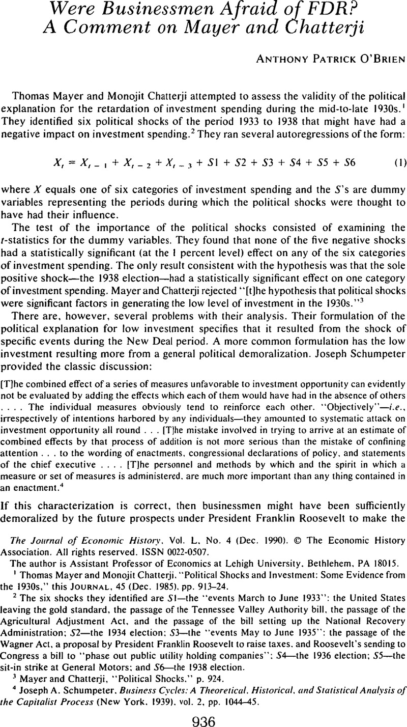
² The six shocks they identified are SI—the “events March to June 1933”: the United States leaving the gold standard, the passage of the Tennessee Valley Authority bill, the passage of the Agricultural Adjustment Act, and the passage of the bill setting up the National Recovery Administration; S2—the 1934 election: S3—the “events May to June 1935”: the passage of the Wagner Act, a proposal by President Franklin Roosevelt to raise taxes, and Roosevelt's sending to Congress a bill to “phase out public utility holding companies”: S4—the 1936 election; S5—the sit-in strike at General Motors; and S6—the 1938 election.

³ Mayer and Chatterji, “Political Shocks,” p. 924.Google Scholar

⁴ Schumpeter, Joseph A., Business Cycles:A Theoretical. Historical, and Statistical Analysis of the Capitalist Process (New York, 1939), vol. 2, pp. 1044–45.Google Scholar

⁵ Even if their procedure of examining the effects of particular episodes is accepted, it is difficult to justify including the second and third quarters of June 1933. They included the period to capture the first spurt of New Deal legislative proposals. However, these months also represent the first two quarters of the recovery. While the recovery is not usually thought of as being investment-led, it would be extraordinary to find a statistically significant decline in investment spending during the first two quarters of a recovery.Google Scholar

⁶ Robert Aaron Gordon wrote: “Business displayed a notable unwillingness to undertake long-term investment projects, either in new directions or in those lines that had chiefly attracted investment funds in the 1920's. The fact that equipment expenditures made a better showing than business construction suggests that firms were willing to make capital expenditures only as necessary to replace and modernize equipment and to meet relatively minor changes in demand.” See Gordon, Robert Aaron, Business Fluctuations (2nd edn., New York, 1961), p. 436.Google Scholar

⁷ Gordon, Robert J.. ed.. The American Business Cycle: Continuity and Change (Chicago. 1986), appendix B. pp. 810–11.CrossRefGoogle Scholar

⁸ One of their categories of investment—electric motors—includes motors as small as I horsepower, raising the suspicion that consumer demand may have been significant for this product.Google Scholar

⁹ Intuitively, this is because forward-looking consumption decisions will have already made use of all of the information contained in previous periods' income values. See Hall, Robert E., “Stochastic Implications of the Life Cycle-Permanent Income Hypothesis: Theory and Evidence,” Journal of Political Economy, 86 (12 1978). pp. 971–87:CrossRefGoogle Scholar and Sargent, Thomas J., Macroeconomic Theory (2nd edn., Boston. 1987), esp. chaps. 9. 12. 14.Google Scholar

¹⁰ Under the permanent income hypothesis, the household maximizes the expected value of an intertemporal utility function subject to an intertemporal budget constraint. The Euler equations for this problem embody the result that the marginal utility of consumption follows a univariate first-order Markov process (or a “random walk”). A direct corollary of this result is that consumption itself follows a random walk and that, therefore, no other variable Granger-causes consumption. Variable X is said to Granger-cause variable Y if in a regression of Yon lagged values of X and lagged values of Y. the coefficients of the lagged values of X are not zero. The test is meant to determine if lagged values of X have any contribution to make in explaining Y once the contribution of lagged values of Y is controlled for. See Granger, C. W. J., “Investigating Causal Relations by Econometric Models and Cross-Spectral Methods,” Econoinerrica, 37 (07 1969), pp. 424–38.CrossRefGoogle Scholar

¹¹ See Andrews, Pauline, “Manufacturing Fixed Investment and the Great Depression” (Ph.D. diss., University of California at Berkeley, 1982), esp. chap. 4. Of course, there is not universal agreement that the Oct. 1929 stock market crash represented an important shock to businessmen's long-term expectations.Google Scholar

¹² The only failure is SI, the dummy for Mar. to Sept. 1933, which, as argued above, should probably not have been included in the analysis.Google Scholar

¹³ See Sims, Christopher A., “Macroeconomics and Reality,” Econometrica, 48 (01 1980), pp. 17–18CrossRefGoogle Scholar, esp. fn. 19. For a discussion of the pitfalls of confusing statistical and economic significance, see McCloskey, Donald N.. The Rhetoric of Economics (Madison, WI, 1985). chap. 9.Google Scholar

¹⁴ In their article Mayer and Chatterji reported only t-statistics. Mayer very promptly and graciously provided me with the coefficient values when I requested them.Google Scholar

¹⁵ Andrews's analysis was carried out for a series on contracts awarded for manufacturing buildings rather than for all nonresidential buildings. Conceivably, the different results she obtained could have been due to this difference in the series analyzed, although it seems unlikely that factors affecting the demand for manufacturing buildings would not also have affected the demand for the remainder of nonresidential buildings in a similar way. Andrews attempted to capture the impact of the stock market crash by specifying four dummy variables: one each for the fourth quarter of 1929 and the first and second quarters of 1930 and one for the five quarters beginning with the third quarter of 1930 and ending with the third quarter of 1931. Andrews engaged in a specification search (pp. 181, 185) in arriving at these definitions for her dummy variables. This is a dubious procedure and the result makes the impact of the shock seem implausibly drawn out. I reran the autoregressions with two additional dummy variable specifications of the crash. In the first specification three dummy variables were included: one each for the fourth quarter of 1929 (Crash 1), the first quarter of 1930 (Crash 2). and the second of 1930 (Crash 3). In the second specification one dummy variable was used for the period from the fourth quarter of 1929 through the second quarter of 1930 (Crash 4). The results, given below, are qualitatively consistent with the results reported in Table 1 and in conflict with the results reported by Andrews. The t-statistics are given in parentheses.Google Scholar