


1. Introduction
Conservative random walks (discrete time) were introduced in [Reference Englander and Volkov8] as a time-inhomogeneous Markov chain
 $X_n$
,
$X_n$
,
 $n=1,2,\dots$
, defined as a process on
$n=1,2,\dots$
, defined as a process on
 $\mathbb{Z}^d$
such that, for a given (non-random) sequence
$\mathbb{Z}^d$
such that, for a given (non-random) sequence
 $p_1,p_2,\dots$
where all
$p_1,p_2,\dots$
where all
 $p_i\in(0,1)$
, the walk at time n with probability
$p_i\in(0,1)$
, the walk at time n with probability
 $p_n$
randomly picks one of the 2d directions parallel to the axis, and otherwise continues moving in the direction it was going before. This walk can be viewed as a generalization of Gillis’ random walk [Reference Gillis9]. An interesting special case studied in [Reference Englander and Volkov8] is when
$p_n$
randomly picks one of the 2d directions parallel to the axis, and otherwise continues moving in the direction it was going before. This walk can be viewed as a generalization of Gillis’ random walk [Reference Gillis9]. An interesting special case studied in [Reference Englander and Volkov8] is when
 $p_n\to 0$
, and in particular when
$p_n\to 0$
, and in particular when
 $p_n\sim n^{-\alpha}$
where
$p_n\sim n^{-\alpha}$
where
 $\alpha\in(0,1]$
; note that the case
$\alpha\in(0,1]$
; note that the case
 $\alpha>1$
is trivial as the walk would make only finitely many turns. The question of recurrence vs. transience of this walk was one of the main questions of that paper.
$\alpha>1$
is trivial as the walk would make only finitely many turns. The question of recurrence vs. transience of this walk was one of the main questions of that paper.
Similar processes have appeared in the literature under different names. Some of the earliest papers which mention a continuous process with memory of this type were probably [Reference Goldstein10, Reference Kac12]. The term persistent random was used in [Reference Cénac, Le Ny, de Loynes and Offret3, Reference Cénac, Le Ny, de Loynes and Offret4]; in these papers some very general criteria of recurrence vs. transience were investigated. A planar motion with just three directions was studied in [Reference Di Crescenzo6]. A book on Markov random flights was recently published [14]. Planar random motions with drifts with four directions/speeds, switching at Poisson times, were studied in [Reference Orsingher and Ratanov17]. Applications of telegraph processes to option pricing can be found in [Reference Ratanov and Kolesnik18]. Characteristic functions of correlated random walks were studied in [Reference Chen and Renshaw5].
The main difference between the conservative random walk and most of the models studied in the literature (except, perhaps, [Reference Vasdekis and Roberts19], which has a more applied focus) is that the underlying process of direction switching is time-inhomogeneous, thus creating various new phenomena. The recurrence/transience of a discrete-space conservative random walk on
 $\mathbb{Z}^1$
was thoroughly studied in [Reference Englander, Volkov and Wang7] (see also the references therein), and we believe that the continuous-time version in one dimension will have very similar features. The establishment of recurrence in one dimension is more or less equivalent to finding that the
$\mathbb{Z}^1$
was thoroughly studied in [Reference Englander, Volkov and Wang7] (see also the references therein), and we believe that the continuous-time version in one dimension will have very similar features. The establishment of recurrence in one dimension is more or less equivalent to finding that the
 $\limsup$
of the process is
$\limsup$
of the process is
 $+\infty$
and the
$+\infty$
and the
 $\liminf$
of the process is
$\liminf$
of the process is
 $-\infty$
, while in higher dimensions the situation is much more intricate. Hence, we concentrate on the case when the dimension of the space is at least 2, except for Theorem 3.1 which deals with the embedded process.
$-\infty$
, while in higher dimensions the situation is much more intricate. Hence, we concentrate on the case when the dimension of the space is at least 2, except for Theorem 3.1 which deals with the embedded process.
Below we formally introduce the two versions of a continuous-time conservative random walk on
 $\mathbb{R}^d$
,
$\mathbb{R}^d$
,
 $d\ge 1$
.
$d\ge 1$
.
1.1. Model A (orthogonal model)
Let
 $\lambda(t)$
be a non-negative function such that
$\lambda(t)$
be a non-negative function such that
 \begin{equation} \Lambda(T) = \int_0^T\lambda(t)\,\mathrm{d}t < \infty \quad \mathrm{for\;all}\;T\ge 0; \qquad \lim_{T\to \infty}\Lambda(T) = \infty.\end{equation}
Let
 $\tau_1<\tau_2<\cdots$
be the consecutive points of an inhomogeneous Poisson point process (PPP) on
$\tau_1<\tau_2<\cdots$
be the consecutive points of an inhomogeneous Poisson point process (PPP) on
 $[0,\infty)$
with rate
$[0,\infty)$
with rate
 $\lambda(t)$
, and
$\lambda(t)$
, and
 $\tau_0=0$
. Then the conditions in (1.1) guarantee that there will be finitely many
$\tau_0=0$
. Then the conditions in (1.1) guarantee that there will be finitely many
 $\tau_i$
in every finite interval, and that
$\tau_i$
in every finite interval, and that
 $\tau_n\to\infty$
. Let
$\tau_n\to\infty$
. Let
 $\textbf{f}_0,\textbf{f}_1,\textbf{f}_2$
be an independent and identically distributed (i.i.d.) sequence of vectors, each of which has a uniform distribution on the set of 2d unit vectors
$\textbf{f}_0,\textbf{f}_1,\textbf{f}_2$
be an independent and identically distributed (i.i.d.) sequence of vectors, each of which has a uniform distribution on the set of 2d unit vectors
 $\{\pm \textbf{e}_1,\pm \textbf{e}_2,\dots, \pm \textbf{e}_d\}$
in
$\{\pm \textbf{e}_1,\pm \textbf{e}_2,\dots, \pm \textbf{e}_d\}$
in
 $\mathbb{R}^d$
.
$\mathbb{R}^d$
.
The (orthogonal, continuous-time) conservative walk generated by the rate function
 $\lambda(\!\cdot\!)$
is a process Z(t),
$\lambda(\!\cdot\!)$
is a process Z(t),
 $t\ge 0$
, in
$t\ge 0$
, in
 $\mathbb{R}^d$
,
$\mathbb{R}^d$
,
 $d\ge 1$
, such that
$d\ge 1$
, such that
 $Z(0)=0$
and at each time
$Z(0)=0$
and at each time
 $\tau_k$
,
$\tau_k$
,
 $k\ge 0$
, the walk starts moving in the direction
$k\ge 0$
, the walk starts moving in the direction
 $\textbf{f}_k$
, and keeps moving in this direction until time
$\textbf{f}_k$
, and keeps moving in this direction until time
 $\tau_{k+1}$
, when it updates its direction. Formally, we define
$\tau_{k+1}$
, when it updates its direction. Formally, we define
 $N(t)=\sup\{k\ge 0\colon\tau_k\le t\}$
as the number of points of the PPP by time t; then
$N(t)=\sup\{k\ge 0\colon\tau_k\le t\}$
as the number of points of the PPP by time t; then
 \begin{align*}Z(t)=\sum_{k=0}^{N(t)-1} (\tau_{k+1}-\tau_{k})\textbf{f}_{k} +(t-\tau_{N(t)})\textbf{f}_{N(t)}.\end{align*}
We can also define the embedded process
 $W_n=Z(\tau_n)$
so that
$W_n=Z(\tau_n)$
so that
 $W(0)=0$
and, for
$W(0)=0$
and, for
 $n\ge 1$
,
$n\ge 1$
,
 $W_n=\sum_{k=0}^{n-1}(\tau_{k+1}-\tau_{k})\textbf{f}_{k}$
. The process Z(t) can be viewed as a continuous equivalent of the conservative random walk introduced in [Reference Englander and Volkov8].
$W_n=\sum_{k=0}^{n-1}(\tau_{k+1}-\tau_{k})\textbf{f}_{k}$
. The process Z(t) can be viewed as a continuous equivalent of the conservative random walk introduced in [Reference Englander and Volkov8].
1.2. Model B (von Mises–Fisher model)
This model is defined similarly to the previous one, except that now the random vectors
 $\textbf{f}_k$
,
$\textbf{f}_k$
,
 $k=1,2,\dots$
, have a uniform distribution on the d-dimensional unit sphere
$k=1,2,\dots$
, have a uniform distribution on the d-dimensional unit sphere
 $\mathcal{S}^{d-1}$
, often called the von Mises–Fisher distribution, instead of just on 2d unit vectors of
$\mathcal{S}^{d-1}$
, often called the von Mises–Fisher distribution, instead of just on 2d unit vectors of
 $\mathbb{R}^d$
.
$\mathbb{R}^d$
.
Note that this model is similar to the ‘random flights’ model studied, e.g., in [Reference Orsingher and De Gregorio16]; however, their results are only for a time-homogeneous Poisson process, unlike our case.
1.3. Aims of this paper
The results that we obtain in the current paper are somewhat different for the two models; however, since they share a lot of common features, certain statements will hold for both of them. The main goal is establishing transience vs. recurrence of the walks, defined as follows.
Definition 1.1. Let
 $\rho\ge 0$
. We say that the walk Z(t) is
$\rho\ge 0$
. We say that the walk Z(t) is
 $\rho$
-recurrent if there is an infinite sequence of times
$\rho$
-recurrent if there is an infinite sequence of times
 $t_1<t_2<\cdots$
, converging to infinity, such that
$t_1<t_2<\cdots$
, converging to infinity, such that
 $Z(t_i)\in[-\rho,\rho]^d$
for all
$Z(t_i)\in[-\rho,\rho]^d$
for all
 $i=1,2,\dots$
We say that the walk Z(t) is transient if it is not
 $\rho$
-recurrent for any
$\rho$
-recurrent for any
 $\rho>0$
, or, equivalently,
$\rho>0$
, or, equivalently,
 $\lim_{t\to\infty}\Vert Z(t)\Vert=\infty$
.
$\lim_{t\to\infty}\Vert Z(t)\Vert=\infty$
.
Recurrence and transience of the embedded process
 $W_n$
are defined analogously, with the exception that instead of
$W_n$
are defined analogously, with the exception that instead of
 $t_1,t_2,t_3,\dots$
in the above definition, we have a strictly increasing sequence of positive integers
$t_1,t_2,t_3,\dots$
in the above definition, we have a strictly increasing sequence of positive integers
 $n_i$
,
$n_i$
,
 $i=1,2,\dots$
Remark 1.1. Note that a priori it is unclear if transience and recurrence are zero–one events; neither can we easily rule out the possibility of ‘intermediate’ situations (e.g.
 $\rho$
-recurrence only for some
$\rho$
-recurrence only for some
 $\rho$
).
$\rho$
).
Our main results, which show transience for two types of rates, are presented in Theorems 3.1, 3.2, 3.3, and 4.1.
2. Preliminaries
Throughout the paper we use the following notation. We write
 $X\sim\mathrm{Poi}(\mu)$
when X has a Poisson distribution with parameter
$X\sim\mathrm{Poi}(\mu)$
when X has a Poisson distribution with parameter
 $\mu>0$
. For any set A,
$\mu>0$
. For any set A,
 $|A|$
denotes its cardinality. For
$|A|$
denotes its cardinality. For
 $x\in\mathbb{R}^d$
,
$x\in\mathbb{R}^d$
,
 $\Vert x\Vert$
denotes the usual Euclidean norm of x.
$\Vert x\Vert$
denotes the usual Euclidean norm of x.
First, we state Kesten’s generalization of the Kolmogorov–Rogozin inequality. Let
 $S_n=\xi_1+\dots+\xi_n$
where the
$S_n=\xi_1+\dots+\xi_n$
where the
 $\xi_i$
are independent, and for any random variable Y define
$\xi_i$
are independent, and for any random variable Y define
 $Q(Y;\;a)=\sup_x \mathbb{P}(Y\in[x,x+a])$
.
$Q(Y;\;a)=\sup_x \mathbb{P}(Y\in[x,x+a])$
.
Lemma 2.1. ([Reference Kesten13].) There exists
 $C>0$
such that, for any real numbers
$C>0$
such that, for any real numbers
 $0<a_1,\dots,a_n\le 2L$
,
$0<a_1,\dots,a_n\le 2L$
,
 \begin{align*} Q(S_n;\;L) \le \frac{CL\sum_{i=1}^n a_i^2(1-Q(\xi_i;\;a_i))Q(\xi_i;\;a_i)}{\big[\sum_{i=1}^n a_i^2(1-Q(\xi_i;\;a_i))\big]^{3/2}}. \end{align*}
Second, if
 $D_1,\dots, D_m$
is a sequence of independent events each with probability p,
$D_1,\dots, D_m$
is a sequence of independent events each with probability p,
 $\varepsilon>0$
, and
$\varepsilon>0$
, and
 $N_D(m)=\mathrm{card}(\{i\in\{1,\dots,m\}\colon D_i\;\mathrm{ occurs}\})=\sum_{i=1}^m\textbf{1}_{D_i}$
, then
$N_D(m)=\mathrm{card}(\{i\in\{1,\dots,m\}\colon D_i\;\mathrm{ occurs}\})=\sum_{i=1}^m\textbf{1}_{D_i}$
, then
 \begin{equation} \mathbb{P}(|N_D(m)-pm| \ge \varepsilon m) \le 2{\mathrm{e}}^{-2\varepsilon^2 m}\end{equation}
by Hoeffding’s inequality (see, e.g., [Reference Hoeffding11]).
Suppose we have an inhomogeneous PPP with rate
 \begin{equation} \lambda(t)=\frac{1}{t^\alpha},\qquad t>0,\end{equation}
where
 $0<\alpha<1$
is constant; thus
$0<\alpha<1$
is constant; thus
 \begin{align*}\Lambda(T)=\int_0^T\lambda(t)\,\mathrm{d}t=\frac{T^{1-\alpha}}{1-\alpha}\end{align*}
and the conditions in (1.1) are fulfilled. Let
 $0<\tau_1<\tau_2<\cdots$
denote the points of the PPP inincreasing order.
$0<\tau_1<\tau_2<\cdots$
denote the points of the PPP inincreasing order.
The following statement is probably known, but for the sake of completeness, we provide its short proof.
Claim 2.1. Let Z be a Poisson random variable with rate
 $\mu>0$
. Then
$\mu>0$
. Then
 \begin{align*} \mathbb{P}\bigg(Z\ge\frac{3\mu}2\bigg) & \le {\mathrm{e}}^{-(({3\ln(3/2)-1})/2)\mu} = {\mathrm{e}}^{-0.108\dots\mu}, \\[5pt] \mathbb{P}\bigg(Z\le\frac{\mu}2\bigg) & \le {\mathrm{e}}^{-(({1-\ln 2})/2)\mu} = {\mathrm{e}}^{-0.153\dots\mu}. \end{align*}
Proof. By the Markov inequality, since
 $\mathbb{E}{\mathrm{e}}^{uZ}={\mathrm{e}}^{\mu({\mathrm{e}}^u-1)}$
, we have, for
$\mathbb{E}{\mathrm{e}}^{uZ}={\mathrm{e}}^{\mu({\mathrm{e}}^u-1)}$
, we have, for
 $u>0$
,
$u>0$
,
 \begin{equation*} \mathbb{P}\bigg(Z\ge\frac{3\mu}2\bigg) \le \mathbb{P}({\mathrm{e}}^{uZ}\ge{\mathrm{e}}^{{3\mu u}/2}) \le {\mathrm{e}}^{-{3\mu u}/2}\mathbb{E}\,{\mathrm{e}}^{uZ} = \exp\!\bigg\{{-}\mu\bigg[\frac{3u}{2}-{\mathrm{e}}^u+1\bigg]\bigg\}. \end{equation*}
Setting
 $u=\ln(3/2)$
yields the first inequality in the claim.
$u=\ln(3/2)$
yields the first inequality in the claim.
For the second inequality, we use
 \begin{equation*} \mathbb{P}\bigg(Z\le \frac{\mu}2\bigg) \le \mathbb{P}({\mathrm{e}}^{-uZ}\ge{\mathrm{e}}^{-{\mu u}/2}) \le {\mathrm{e}}^{{\mu u}/2}\mathbb{E}\,{\mathrm{e}}^{-uZ} = \exp\!\bigg\{{-}\mu\bigg[{-}\frac{u}2-{\mathrm{e}}^{-u}+1\bigg]\bigg\}. \end{equation*}
Now let
 $u=\ln 2$
.
$u=\ln 2$
.
Lemma 2.2. Suppose that the rate of the PPP is given by (2.2). For some
 $c_1>c_0>0$
, depending on
$c_1>c_0>0$
, depending on
 $\alpha$
only,
$\alpha$
only,
 \begin{equation*} \mathbb{P}(\tau_k \le c_0 k^{{1}/({1-\alpha})}) \le {\mathrm{e}}^{-k/15}; \qquad \mathbb{P}(\tau_k \ge c_1 k^{{1}/({1-\alpha})}) \le {\mathrm{e}}^{-k/15}. \end{equation*}
Proof. Recall that N(s) denotes the number of points of the PPP by time s. Then
 $N(s)\sim\mathrm{Poi}(\Lambda(s))$
, and
$N(s)\sim\mathrm{Poi}(\Lambda(s))$
, and
 $\mathbb{P}(\tau_k\le s)=\mathbb{P}(N(s)\ge k)$
. Let
$\mathbb{P}(\tau_k\le s)=\mathbb{P}(N(s)\ge k)$
. Let
 $T_n=\Lambda^{(-1)}(n)=\sqrt[1-\alpha]{(1-\alpha)n}$
. Noting that
$T_n=\Lambda^{(-1)}(n)=\sqrt[1-\alpha]{(1-\alpha)n}$
. Noting that
 $N(T_n)\sim\mathrm{Poi}(n)$
for all n, we have
$N(T_n)\sim\mathrm{Poi}(n)$
for all n, we have
 \begin{align*} \mathbb{P}(\tau_k\le T_{2k/3}) = \mathbb{P}(N(T_{2k/3})\ge k) = \mathbb{P}\bigg(Z\ge\frac32\mu\bigg) \le {\mathrm{e}}^{-0.072\,13\dots k} \end{align*}
by Claim 2.1, with
 $Z\sim\mathrm{Poi}(\mu)$
where
$Z\sim\mathrm{Poi}(\mu)$
where
 $\mu=2k/3$
. Similarly,
$\mu=2k/3$
. Similarly,
 \begin{align*} \mathbb{P}(\tau_k\ge T_{2k}) = \mathbb{P}(N(T_{2k})\le k) \le \mathbb{P}\bigg(Z\le\frac12\mu\bigg) \le {\mathrm{e}}^{-0.306\,85\dots k} \end{align*}
by Claim 2.1, with
 $Z\sim\mathrm{Poi}(\mu)$
where
$Z\sim\mathrm{Poi}(\mu)$
where
 $\mu=2k$
. Note that
$\mu=2k$
. Note that
 $0.072\,13>\frac1{15}$
,
$0.072\,13>\frac1{15}$
,
 $0.306\,85>\frac1{15}$
. Now the statement follows with
$0.306\,85>\frac1{15}$
. Now the statement follows with
 $c_0=\sqrt[1-\alpha]{2(1-\alpha)/3}$
and
$c_0=\sqrt[1-\alpha]{2(1-\alpha)/3}$
and
 $c_1=\sqrt[1-\alpha]{2(1-\alpha)}$
.
$c_1=\sqrt[1-\alpha]{2(1-\alpha)}$
.
3. Analysis of Model A
Theorem 3.1. Let
 $d=1$
,
$d=1$
,
 $\alpha\in\big(\frac13,1\big)$
, and the rate be given by (2.2). Then the embedded walk
$\alpha\in\big(\frac13,1\big)$
, and the rate be given by (2.2). Then the embedded walk
 $W_n$
is transient almost surely (a.s.).
$W_n$
is transient almost surely (a.s.).
Proof. Assume without loss of generality that n is even. We will show that for any
 $\rho>0$
the walk
$\rho>0$
the walk
 $W_n$
visits
$W_n$
visits
 $[-\rho,\rho]$
finitely often a.s. With probabilities close to 1, both the events
$[-\rho,\rho]$
finitely often a.s. With probabilities close to 1, both the events
 \begin{equation} \mathcal{E}_1 = \big\{\tau_{n/2} \ge c_0(n/2)^{{1}/({1-\alpha})}\big\}, \qquad \mathcal{E}_2 = \big\{\tau_{n} \le c_1 n^{{1}/({1-\alpha})}\big\} \end{equation}
occur; indeed,
 \begin{equation} \mathbb{P}(\mathcal{E}_1^\mathrm{c}) \le {\mathrm{e}}^{-n/30}, \qquad \mathbb{P}(\mathcal{E}_2^\mathrm{c}) \le {\mathrm{e}}^{-n/15} \end{equation}
by Lemma 2.2.
Since the rate
 $\lambda(t)=t^{-\alpha}$
of the Poisson process is monotonically decreasing, the random variables
$\lambda(t)=t^{-\alpha}$
of the Poisson process is monotonically decreasing, the random variables
 $\tau_i - \tau_{i-1}$
,
$\tau_i - \tau_{i-1}$
,
 $n/2\le i\le n$
, under the condition stated in the event
$n/2\le i\le n$
, under the condition stated in the event
 $\mathcal{E}_1$
, are stochastically larger than i.i.d. exponential random variables
$\mathcal{E}_1$
, are stochastically larger than i.i.d. exponential random variables
 $\zeta_i$
with rates equal to
$\zeta_i$
with rates equal to
 $[c_0(n/2)^{1/{1-\alpha}}]^\alpha=\tilde c_0 n^{-{\alpha}/({1-\alpha})}$
for some
$[c_0(n/2)^{1/{1-\alpha}}]^\alpha=\tilde c_0 n^{-{\alpha}/({1-\alpha})}$
for some
 $\tilde c_0>0$
. For
$\tilde c_0>0$
. For
 $\zeta$
, there exists
$\zeta$
, there exists
 $\beta=\beta(c_0,\alpha)>0$
such that
$\beta=\beta(c_0,\alpha)>0$
such that
 \begin{align*} \mathbb{P}\big(\zeta_i>\beta n^{{\alpha}/({1-\alpha})}\big) = \exp\!\big({-}\tilde c_0 n^{-{\alpha}/({1-\alpha})}\cdot\beta n^{{\alpha}/({1-\alpha})}\big) = {\mathrm{e}}^{-\tilde c_0 \beta} = \frac{2}{3}. \end{align*}
Let
 $I_n=\big\{i\in[n/2,n]\colon\;i\;\mathrm{is\;even},\,\tau_i-\tau_{i-2}>\beta n^{{\alpha}/({1-\alpha})}\big\}$
, and note that
$I_n=\big\{i\in[n/2,n]\colon\;i\;\mathrm{is\;even},\,\tau_i-\tau_{i-2}>\beta n^{{\alpha}/({1-\alpha})}\big\}$
, and note that
 $\mathrm{card}(I_n)\le n/4$
. Then, since
$\mathrm{card}(I_n)\le n/4$
. Then, since
 $\tau_i-\tau_{i-2}>\tau_i-\tau_{i-1}$
, by stochastic monotonicity and Hoeffding’s inequality (2.1) with
$\tau_i-\tau_{i-2}>\tau_i-\tau_{i-1}$
, by stochastic monotonicity and Hoeffding’s inequality (2.1) with
 $m=n/4$
,
$m=n/4$
,
 $p=\frac23$
, and
$p=\frac23$
, and
 $\varepsilon=\frac23-\frac12=\frac16$
,
$\varepsilon=\frac23-\frac12=\frac16$
,
 \begin{align} \mathbb{P}\bigg(\!\mathrm{card}(I_n) <\frac12\cdot\frac{n}{4}\mid\mathcal{E}_1\bigg) & \le \mathbb{P}\bigg(\!\mathrm{card}\big(\big\{i\in[n/2,n]\colon\;\textit{i}\;\mathrm{is\;even},\, \zeta_i>\beta n^{{\alpha}/({1-\alpha})}\big\}\big)< \frac{n}{8}\bigg) \nonumber \\[5pt] & \le 2{\mathrm{e}}^{-n/72}. \end{align}
Let
 $J_n=\{i\in I_n\colon\textbf{f}_{i-1}=-\textbf{f}_{i-2}\}$
. Since the
$J_n=\{i\in I_n\colon\textbf{f}_{i-1}=-\textbf{f}_{i-2}\}$
. Since the
 $\textbf{f}_i$
are i.i.d. and independent of
$\textbf{f}_i$
are i.i.d. and independent of
 $\{\tau_1,\tau_2,\dots\}$
, and
$\{\tau_1,\tau_2,\dots\}$
, and
 $\mathbb{P}(\textbf{f}_{i-1}={-}\textbf{f}_i)=\frac12$
, on the event
$\mathbb{P}(\textbf{f}_{i-1}={-}\textbf{f}_i)=\frac12$
, on the event
 $\{\mathrm{card}(I_n)\ge n/8\}$
we have, by (2.1) with
$\{\mathrm{card}(I_n)\ge n/8\}$
we have, by (2.1) with
 $m=\mathrm{card}(I_n)$
,
$m=\mathrm{card}(I_n)$
,
 $p=\frac12$
, and
$p=\frac12$
, and
 $\varepsilon=\frac{1}{34}$
,
$\varepsilon=\frac{1}{34}$
,
 \begin{align} \mathbb{P}\bigg(\!\mathrm{card}(J_n)<\frac{n}{17}\mid\mathrm{card}(I_n)\ge\frac{n}{8}\bigg) & \le \mathbb{P}\bigg(\bigg|\mathrm{card}(J_n)-\frac{\mathrm{card}(I_n)}2\bigg| > \frac{\mathrm{card}(I_n)}{34}\mid\mathrm{card}(I_n)\ge\frac{n}{8}\bigg) \nonumber \\[5pt] & \le 2\exp\!\bigg\{{-}2\cdot\frac{1}{34^2}\cdot\frac{n}{8}\bigg\} = 2{\mathrm{e}}^{-c_* n}, \end{align}
where
 $c_*=1/4624$
.
$c_*=1/4624$
.
Our proof will rely on conditioning over the even stopping times, i.e. on the event
 $\mathcal{D}=\mathcal{D}_0\cap\mathcal{D}_1\cap\mathcal{E}_2$
, where
$\mathcal{D}=\mathcal{D}_0\cap\mathcal{D}_1\cap\mathcal{E}_2$
, where
 \begin{equation*} \mathcal{D}_0 = \big\{\tau_{n/2}=t_{n/2},\tau_{n/2+2}=t_{n/2+2},\dots,\tau_n=t_n\big\}, \qquad \mathcal{D}_1 = \{\mathrm{card}(J_n)\ge n/17\}\cap\mathcal{E}_1 \end{equation*}
for some strictly increasing sequence
 $0<t_{n/2}<t_{n/2+2}<\dots<t_n$
. Note that
$0<t_{n/2}<t_{n/2+2}<\dots<t_n$
. Note that
 \begin{align} \mathbb{P}(\mathcal{D}_1^\mathrm{c}) & \le \mathbb{P}(\mathcal{E}_1^\mathrm{c}) + \mathbb{P}\bigg(\!\mathrm{card}(J_n)<\frac{n}{17}\mid\mathcal{E}_1\bigg) \nonumber \\[5pt] & \le \mathbb{P}(\mathcal{E}_1^\mathrm{c}) + \mathbb{P}\bigg(\!\mathrm{card}(J_n)<\frac{n}{17}\mid\mathrm{card}(I_n)\ge\frac{n}{8},\mathcal{E}_1\bigg) + \mathbb{P}\bigg(\!\mathrm{card}(I_n)<\frac{n}{8}\mid\mathcal{E}_1\bigg) \nonumber \\[5pt] & \le {\mathrm{e}}^{-n/30} + 2{\mathrm{e}}^{-c_* n} + 2{\mathrm{e}}^{-n/72} \le 5{\mathrm{e}}^{-c_*n} \end{align}
We denote the ith step of the embedded walk by
 $X_i=W_i-W_{i-1}$
,
$X_i=W_i-W_{i-1}$
,
 $i=1,2,\dots$
, and
$i=1,2,\dots$
, and
 \begin{align*} \xi_{i}\;:\!=\;X_{i-1}+X_{i}=(\tau_{i-1}-\tau_{i-2})\textbf{f}_{i-2}+(\tau_{i}-\tau_{i-1})\textbf{f}_{i-1}. \end{align*}
Conditioned on
 $\mathcal{D}$
, the random variables
$\mathcal{D}$
, the random variables
 $\xi_2,\xi_4,\xi_6,\dots$
are then independent.
$\xi_2,\xi_4,\xi_6,\dots$
are then independent.
Lemma 3.1. For
 $i\in J_n$
,
$i\in J_n$
,
 $\sup_{x\in\mathbb{R}}\mathbb{P}(\xi_i\in[x-\rho,x+\rho]\mid\mathcal{D}) \leq {c\rho}/n^{\alpha/({1-\alpha})}$
for some
$\sup_{x\in\mathbb{R}}\mathbb{P}(\xi_i\in[x-\rho,x+\rho]\mid\mathcal{D}) \leq {c\rho}/n^{\alpha/({1-\alpha})}$
for some
 $c=c(\alpha)>0$
.
$c=c(\alpha)>0$
.
Proof of Lemma
3.1. Given
 $\tau_{i-2}=t_{i-2}$
and
$\tau_{i-2}=t_{i-2}$
and
 $\tau_i=t_i$
,
$\tau_i=t_i$
,
 $\tau_{i-1}$
has the distribution of the only point of the PPP on
$\tau_{i-1}$
has the distribution of the only point of the PPP on
 $[t_{i-2},t_i]$
with rate
$[t_{i-2},t_i]$
with rate
 $\lambda(t)$
conditioned on the fact that there is exactly one point in this interval. Hence, the conditional density of
$\lambda(t)$
conditioned on the fact that there is exactly one point in this interval. Hence, the conditional density of
 $\tau_{i-1}$
is given by
$\tau_{i-1}$
is given by
 \begin{align*} f_{\tau_{i-1}\mid\mathcal{D}}(x) = \begin{cases} \dfrac{\lambda(t)}{\int_{t_{i-2}}^{t_i}\lambda(u)\,\mathrm{d}u} & \mathrm{if }\;x\in[t_{i-2},t_i], \\[5pt] 0 & \mathrm{otherwise.} \end{cases} \end{align*}
Assume without loss of generality that
 $X_{i-1}>0>X_i$
(recall that
$X_{i-1}>0>X_i$
(recall that
 $i\in J_n$
). Then
$i\in J_n$
). Then
 \begin{align*} \xi_i=[\tau_{i-1}-\tau_{i-2}]-[\tau_{i}-\tau_{i-1}]=2\tau_{i-1}-(t_{i-2}+t_i) \end{align*}
so that the maximum of the conditional density of
 $\xi_i$
equals one-half of the maximum of the conditional density of
$\xi_i$
equals one-half of the maximum of the conditional density of
 $\tau_{i-1}$
. At the same time, since
$\tau_{i-1}$
. At the same time, since
 $\lambda$
is a decreasing function,
$\lambda$
is a decreasing function,
 \begin{align*} \sup_{x\in\mathbb{R}}f_{\tau_{i-1}\mid\mathcal{D}}(x) & = \frac{\lambda(t_{i-2})}{\int_{t_{i-2}}^{t_i}\lambda(u)\,\mathrm{d}u} \le \frac{\lambda(t_{i-2})}{(t_i-t_{i-2})\lambda(t_{i})} \le \frac{\lambda(t_{i-2})}{\beta n^{{\alpha}/({1-\alpha})}\lambda(t_{i})} = \frac{1}{\beta n^{{\alpha}/({1-\alpha})}} \cdot \bigg(\frac{t_i}{t_{i-2}}\bigg)^\alpha \\[5pt] & \le \frac{1}{\beta n^{{\alpha}/({1-\alpha})}} \cdot \bigg(\frac{\tau_n}{\tau_{n/2}}\bigg)^\alpha \le \frac{1}{\beta n^{{\alpha}/({1-\alpha})}} \cdot \bigg(\frac{c_1}{c_0 2^{-{1}/({1-\alpha})}}\bigg)^\alpha \end{align*}
since the events
 $\mathcal{E}_1$
and
$\mathcal{E}_1$
and
 $\mathcal{E}_2$
occur. This implies the stated result with
$\mathcal{E}_2$
occur. This implies the stated result with
 $c=\beta^{-1}(c_0^{-1}c_1\sqrt[1-\alpha]{2})^\alpha$
.
$c=\beta^{-1}(c_0^{-1}c_1\sqrt[1-\alpha]{2})^\alpha$
.
Now we divide
 $W_n$
into two portions:
$W_n$
into two portions:
 \begin{equation*} A = \sum_{i\in J_n}\xi_i, \qquad B = W_n - A = \sum_{i\in\{2,4,\dots,n\}\setminus J_n}\xi_i. \end{equation*}
Lemma 3.2. For some
 $C=C(\alpha,\rho)>0$
,
$C=C(\alpha,\rho)>0$
,
 \begin{align*} \sup_{x\in\mathbb{R}}\mathbb{P}(A\in[x-\rho,x+\rho]\mid\mathcal{D}) \leq \frac{C}{n^{{\alpha}/({1-\alpha})+1/2}}. \end{align*}
Proof of Lemma
3.2. The result follows immediately from Lemma 2.1 with
 $a_i\equiv 2\rho=L$
, using Lemma 3.1 and the fact that
$a_i\equiv 2\rho=L$
, using Lemma 3.1 and the fact that
 $\mathrm{card}(J_n)\ge n/17$
.
$\mathrm{card}(J_n)\ge n/17$
.
So,
 \begin{align*} \mathbb{P}(|W_n|\le\rho\mid\mathcal{D}) & = \mathbb{P}(A+B\in[-\rho,\rho]\mid\mathcal{D}) = \int\mathbb{P}(A+b\in[-\rho,\rho]\mid\mathcal{D})f_{B|\mathcal{D}}(b)\,\mathrm{d}b \\[5pt] & \le \int\sup_x\mathbb{P}(A\in[x-\rho,x+\rho]\mid\mathcal{D})f_{B|\mathcal{D}}(b)\,\mathrm{d}b \le \frac{C}{n^{{\alpha}/({1-\alpha})+1/2}}, \end{align*}
where
 $f_{B|\mathcal{D}}(\!\cdot\!)$
is the density of B conditional on
$f_{B|\mathcal{D}}(\!\cdot\!)$
is the density of B conditional on
 $\mathcal{D}$
.
$\mathcal{D}$
.
Finally, using (3.2) and (3.5),
 \begin{align*} \mathbb{P}(W_n\in[-\rho,\rho]) \le \mathbb{P}(W_n\in[-\rho,\rho]\mid\mathcal{D}) + \mathbb{P}(\mathcal{D}_1^\mathrm{c}) + \mathbb{P}(\mathcal{E}_2^\mathrm{c}) \le \frac{C}{n^{{\alpha}/({1-\alpha})+1/2}} + 5{\mathrm{e}}^{-c_* n} + {\mathrm{e}}^{-n/15}, \end{align*}
which is summable over n, so we can apply the Borel–Cantelli lemma to show that
 $\{|W_n|\le\rho\}$
occurs finitely often a.s.
$\{|W_n|\le\rho\}$
occurs finitely often a.s.
Theorem 3.2. Let
 $d\ge 2$
,
$d\ge 2$
,
 $\alpha\in(0,1)$
, and the rate of the PPP be given by (2.2). Then Z(t) is transient a.s.
$\alpha\in(0,1)$
, and the rate of the PPP be given by (2.2). Then Z(t) is transient a.s.
Remark 3.1. This result also holds for
 $\alpha=1$
, and the proof is more or less identical to that of [Reference Englander and Volkov8, Theorem 5.2], once we establish that, a.s.,
$\alpha=1$
, and the proof is more or less identical to that of [Reference Englander and Volkov8, Theorem 5.2], once we establish that, a.s.,
 $\tau_n>{\mathrm{e}}^{cn}$
for some
$\tau_n>{\mathrm{e}}^{cn}$
for some
 $c>0$
and all large n; the latter follows from arguments similar to Lemma 2.2.
$c>0$
and all large n; the latter follows from arguments similar to Lemma 2.2.
Proof of Theorem
3.2. We provide the proof only for the case
 $d=2$
and
$d=2$
and
 $\rho=1$
; it can be easily generalized for all
$\rho=1$
; it can be easily generalized for all
 $d\ge 3$
and
$d\ge 3$
and
 $\rho>0$
. Denote the coordinates of the embedded walk by
$\rho>0$
. Denote the coordinates of the embedded walk by
 $X_n$
and
$X_n$
and
 $Y_n$
; thus
$Y_n$
; thus
 $W_n=(X_n,Y_n)\in\mathbb{R}^2$
. Fix some small
$W_n=(X_n,Y_n)\in\mathbb{R}^2$
. Fix some small
 $\varepsilon>0$
and consider the event
$\varepsilon>0$
and consider the event
 $\mathcal{R}_n=\{Z(t)\in[-1,1]^2\;\mathrm{ for\;some }\;t\in(\tau_n,\tau_{n+1}]\}$
. We will show that events
$\mathcal{R}_n=\{Z(t)\in[-1,1]^2\;\mathrm{ for\;some }\;t\in(\tau_n,\tau_{n+1}]\}$
. We will show that events
 $\mathcal{R}_n$
occur finitely often a.s., thus ensuring the transience of Z(t).
$\mathcal{R}_n$
occur finitely often a.s., thus ensuring the transience of Z(t).
For the walk Z(t) to hit
 $[-\rho,\rho]^2$
between times
$[-\rho,\rho]^2$
between times
 $\tau_n$
and
$\tau_n$
and
 $\tau_{n+1}$
, we have to have either
$\tau_{n+1}$
, we have to have either
-
•
 $|X_n|\le\rho$
,
$\textbf{f}_n=-\mathrm{sign}(Y_n)\textbf{e}_2$
, and
$\tau_{n+1}-\tau_n\ge|Y_n|-1$
, or
$|X_n|\le\rho$
,
$\textbf{f}_n=-\mathrm{sign}(Y_n)\textbf{e}_2$
, and
$\tau_{n+1}-\tau_n\ge|Y_n|-1$
, or -
•
$|Y_n|\le\rho$
,
$\textbf{f}_n=-\mathrm{sign}(X_n)\textbf{e}_1$
, and
$\tau_{n+1}-\tau_n\ge|X_n|-1$


(see Figure 1.)
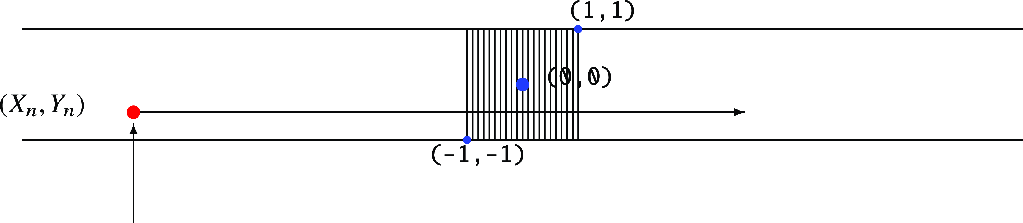
Figure 1. Model A: Recurrence of conservative random walk on
 $\mathbb{R}^2$
.
$\mathbb{R}^2$
.
Using the fact that the
 $\textbf{f}_n$
are independent of anything, we get
$\textbf{f}_n$
are independent of anything, we get
 \begin{align*} \mathbb{P}(\mathcal{R}_n) \le \frac14\mathbb{P}(|X_n|\le\rho,\,\tau_{n+1}-\tau_n\ge|Y_n|-1) + \frac14\mathbb{P}(|Y_n|\le\rho,\,\tau_{n+1}-\tau_n\ge|X_n|-1). \end{align*}
We will show that
 $\mathbb{P}(|X_n|\le\rho,\,|Y_n|\le\tau_{n+1}-\tau_n+1)$
is summable in n (and the same holds for the other summand by symmetry), hence by the Borel–Cantelli lemma that
$\mathbb{P}(|X_n|\le\rho,\,|Y_n|\le\tau_{n+1}-\tau_n+1)$
is summable in n (and the same holds for the other summand by symmetry), hence by the Borel–Cantelli lemma that
 $\mathcal{R}_n$
occurs finitely often a.s.
$\mathcal{R}_n$
occurs finitely often a.s.
Lemma 3.3. Assume that
 $\varepsilon\in(0,1)$
. Then there exists
$\varepsilon\in(0,1)$
. Then there exists
 $c_1^*=c_1^*(\varepsilon)$
such that, for all sufficiently large n,
$c_1^*=c_1^*(\varepsilon)$
such that, for all sufficiently large n,
 $\mathbb{P}\big(\tau_{n+1}-\tau_n+1 \ge n^{{\alpha}/({1-\alpha})+\varepsilon}\big) \le 3{\mathrm{e}}^{-c_1^* n^\varepsilon}$
.
$\mathbb{P}\big(\tau_{n+1}-\tau_n+1 \ge n^{{\alpha}/({1-\alpha})+\varepsilon}\big) \le 3{\mathrm{e}}^{-c_1^* n^\varepsilon}$
.
Proof of Lemma
3.3. For
 $s,t\ge 0$
,
$s,t\ge 0$
,
 \begin{align*} \mathbb{P}(\tau_{n+1}-\tau_n\ge s\mid \tau_n=t) = {\mathrm{e}}^{-[\Lambda(t+s)-\Lambda(t)]} = \exp\!\bigg\{{-}\frac{(t+s)^{1-\alpha}-t^{1-\alpha}}{1-\alpha}\bigg\}, \end{align*}
so if
 $t<c_1 n^{1/({1-\alpha})}$
, where
$t<c_1 n^{1/({1-\alpha})}$
, where
 $c_1$
is the constant from Lemma 2.2, and
$c_1$
is the constant from Lemma 2.2, and
 $s=n^{{\alpha}/({1-\alpha})+\varepsilon}-1 = o(n^{1/({1-\alpha})})$
, we have
$s=n^{{\alpha}/({1-\alpha})+\varepsilon}-1 = o(n^{1/({1-\alpha})})$
, we have
 \begin{align*} \mathbb{P}(\tau_{n+1}-\tau_n \ge s \mid \tau_n=t) & \le \exp\!\bigg\{{-}\frac{(c_1 n^{1/({1-\alpha})}+s)^{1-\alpha}-c_1^{1-\alpha} n}{1-\alpha}\bigg\} \\[5pt] & \le \exp\!\bigg\{{-}\frac{nc_1^{1-\alpha}}{1-\alpha}\bigg[\bigg(1+\frac{n^{{\alpha}/({1-\alpha})+\varepsilon}-1} {c_1 n^{1/({1-\alpha})}}\bigg)^{1-\alpha}-1\bigg]\bigg\} \\[5pt] & = \exp\!\bigg\{{-}\frac{n^\varepsilon(1+o(1))}{c_1^{\alpha}}\bigg\}. \end{align*}
Consequently, using Lemma 2.2,
 \begin{align} \mathbb{P}\big(\tau_{n+1}-\tau_n \ge n^{{\alpha}/({1-\alpha})+\varepsilon}-1\big) & \le \mathbb{P}\big(\tau_{n+1}-\tau_n \ge n^{{\alpha}/({1-\alpha})+\varepsilon}-1\mid\tau_n<c_1 n^{1/({1-\alpha})}\big) \nonumber \\[5pt] & \quad + \mathbb{P}\big(\tau_n \ge c_1 n^{1/({1-\alpha})}\big) \nonumber \\[5pt] & \le {\mathrm{e}}^{-c_1^* n^\varepsilon} + {\mathrm{e}}^{-n/15} \le 2{\mathrm{e}}^{-c_1^* n^\varepsilon} \end{align}
for some
 $c_1^*\in\big(0,\frac{1}{15}\big)$
.
$c_1^*\in\big(0,\frac{1}{15}\big)$
.
Now we will modify the proof of Theorem 3.1 slightly to adapt to our needs. Let the events
 $\mathcal{E}_1$
and
$\mathcal{E}_1$
and
 $\mathcal{E}_2$
be the same as in the proof of Theorem 3.1. We will also use the set
$\mathcal{E}_2$
be the same as in the proof of Theorem 3.1. We will also use the set
 $I_n$
, but instead of
$I_n$
, but instead of
 $J_n$
we introduce the sets
$J_n$
we introduce the sets
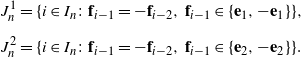 \begin{align*} J_n^1 & = \{i\in I_n\colon\textbf{f}_{i-1}=-\textbf{f}_{i-2},\, \textbf{f}_{i-1}\in\{\textbf{e}_1,-\textbf{e}_1\}\}, \\[5pt] J_n^2 & = \{i\in I_n\colon\textbf{f}_{i-1}=-\textbf{f}_{i-2},\,\textbf{f}_{i-1}\in\{\textbf{e}_2,-\textbf{e}_2\}\}. \end{align*}
Similarly to the proof of Theorem 3.1, inequality (3.5), we immediately obtain that
 \begin{equation} \begin{split} \mathbb{P}(\mathrm{card}(J_n^1) \le n/34) & \le \mathbb{P}(\mathrm{card}(J_n^1) \le n/34\mid\mathcal{E}_1) + \mathbb{P}(\mathcal{E}_1^\mathrm{c}) \le 6{\mathrm{e}}^{-c'_{\!\!\ast}n}, \\[5pt] \mathbb{P}(\mathrm{card}(J_n^2) \le n/34) & \le \mathbb{P}(\mathrm{card}(J_n^2) \le n/34\mid\mathcal{E}_1) + \mathbb{P}(\mathcal{E}_1^\mathrm{c}) \le 6{\mathrm{e}}^{-c'_{\!\!\ast}n} \end{split} \end{equation}
for some
 $c'_{\!\!\ast}>0$
.
$c'_{\!\!\ast}>0$
.
Fix a deterministic sequence of unit vectors
 $\textbf{g}_1,\dots,\textbf{g}_n$
such that each
$\textbf{g}_1,\dots,\textbf{g}_n$
such that each
 $\textbf{g}_i\in\{\pm\textbf{e}_1,\pm\textbf{e}_2\}$
. We now also define the event
$\textbf{g}_i\in\{\pm\textbf{e}_1,\pm\textbf{e}_2\}$
. We now also define the event
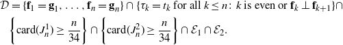 \begin{align*}\mathcal{D}&=\{\textbf{f}_1=\textbf{g}_1,\dots,\textbf{f}_n=\textbf{g}_n\}\cap\{\tau_k=t_k\text{ for all } k\le n\colon k\text{ is even or }\textbf{f}_k\perp \textbf{f}_{k+1}\} \cap \\& \bigg\{\mathrm{card}({J^1_n})\ge \frac{n}{34}\bigg\}\cap \bigg\{\mathrm{card}({J^2_n})\ge \frac{n}{34}\bigg\}\cap \mathcal{E}_1 \cap \mathcal{E}_2.\end{align*}
Therefore, repeating the previous arguments for each of the horizontal and vertical components of
 $W_n$
, we immediately obtain
$W_n$
, we immediately obtain
 \begin{equation*} \mathbb{P}(|X_n|\le1\mid\mathcal{D}) \le \frac{C}{n^{{\alpha}/({1-\alpha})+1/2}}, \qquad \sup_{x\in\mathbb{R}}\mathbb{P}(|Y_n-x|\le1\mid\mathcal{D}) \le \frac{C}{n^{{\alpha}/({1-\alpha})+1/2}}. \end{equation*}
The second inequality implies that
 \begin{align*} \mathbb{P}(|Y_n| \le n^{{\alpha}/({1-\alpha})+\varepsilon} \mid \mathcal{D}) \le n^{{\alpha}/({1-\alpha})+\varepsilon}\cdot\frac{C}{n^{{\alpha}/({1-\alpha})+1/2}} = \frac{C}{n^{1/2-\varepsilon}}. \end{align*}
Now, by Lemma 3.3,
 \begin{align*} \mathbb{P}(|X_n|\le 1,\, & |Y_n|\le \tau_{n+1}-\tau_n+1) \\[5pt] & \le \mathbb{P}\big(|X_n|\le1,|Y_n|\le\tau_{n+1}-\tau_n+1 \mid \tau_{n+1}-\tau_n+1\le n^{{\alpha}/({1-\alpha})+\varepsilon}\big) \\[5pt] & \quad + \mathbb{P}\big(\tau_{n+1}-\tau_n+1\ge n^{{\alpha}/({1-\alpha})+\varepsilon}\big) \\[5pt] & \le \mathbb{P}\big(|X_n|\le1,|Y_n|\le n^{{\alpha}/({1-\alpha})+\varepsilon}\big) + 3{\mathrm{e}}^{-c_1^*n^\varepsilon}. \end{align*}
Observing that
 $X_n$
and
$X_n$
and
 $Y_n$
are actually independent given
$Y_n$
are actually independent given
 $\mathcal{D}$
, we conclude that
$\mathcal{D}$
, we conclude that
 \begin{align*} \mathbb{P}\big(|X_n|\le1,|Y_n|\le n^{{\alpha}/({1-\alpha})+\varepsilon}\big) & \le \mathbb{P}\big(|X_n|\le1,|Y_n|\le n^{{\alpha}/({1-\alpha})+\varepsilon}\mid\mathcal{D}\big) \\[5pt] & \quad + \mathbb{P}\bigg(\!\mathrm{card}(J_n^1)<\frac{n}{34}\;\mathrm{ or }\; \mathrm{card}(J_n^1)<\frac{n}{34}\bigg) + \mathbb{P}(\mathcal{E}_1^\mathrm{c}) + \mathbb{P}(\mathcal{E}_2^\mathrm{c}) \\[5pt] & \le \frac{C}{n^{{\alpha}/({1-\alpha})+1/2}}\cdot\frac{C}{n^{1/2-\varepsilon}} + 12{\mathrm{e}}^{-c'_{\!\!\ast} n} + {\mathrm{e}}^{-n/15} + {\mathrm{e}}^{-n/15} \\[5pt] & = \frac{C^2+o(1)}{n^{1+[{\alpha}/({1-\alpha})-\varepsilon]}} \end{align*}
by (3.2) and (3.7). Assuming
 $\varepsilon\in(0,{\alpha}/({1-\alpha}))$
, the right-hand side is summable, and thus
$\varepsilon\in(0,{\alpha}/({1-\alpha}))$
, the right-hand side is summable, and thus
 $\mathbb{P}(|X_n|\le\rho,|Y_n|-1\le\tau_{n+1}-\tau_n)$
is also summable in n.
$\mathbb{P}(|X_n|\le\rho,|Y_n|-1\le\tau_{n+1}-\tau_n)$
is also summable in n.
Theorem 3.3. Let
 $d\geq2$
, and the rate be given by
$d\geq2$
, and the rate be given by
 \begin{align} \lambda(t) = \begin{cases} \dfrac{1}{(\!\ln{t})^\beta}, & t\ge {\mathrm{e}}; \\[5pt] 0, & \textit{otherwise}. \end{cases} \end{align}
Then Z(t) is transient as long as
 $\beta >2$
.
$\beta >2$
.
Proof. The proof is analogous to the proof of Theorem 3.2; we will only indicate how that proof should be modified for this case. As before, we assume that
 $\rho=1$
and
$\rho=1$
and
 $d=2$
, without loss of generality. First, we prove the following lemma.
$d=2$
, without loss of generality. First, we prove the following lemma.
Lemma 3.4. Let
 $\Lambda(T)=\int_0^T\lambda(s)\,\mathrm{d}s = \int_{\mathrm{e}}^T{\mathrm{d}s}/{(\!\ln s)^\beta}$
. Then
$\Lambda(T)=\int_0^T\lambda(s)\,\mathrm{d}s = \int_{\mathrm{e}}^T{\mathrm{d}s}/{(\!\ln s)^\beta}$
. Then
 \begin{align*} \lim_{T\to\infty}\frac{\Lambda(T)}{T(\!\ln T)^{-\beta}} = 1. \end{align*}
Proof of Lemma
3.4. Fix an
 $\varepsilon\in(0,1)$
. Then
$\varepsilon\in(0,1)$
. Then
 \begin{align*} \Lambda(T) = \int_{\mathrm{e}}^T\frac{\mathrm{d}s}{(\!\ln s)^\beta} = \int_{\mathrm{e}}^{T^{1-\varepsilon}}\frac{\mathrm{d}s}{(\!\ln s)^\beta} + \int_{T^{1-\varepsilon}}^T\frac{\mathrm{d}s}{(\!\ln s)^\beta}< T^{1-\varepsilon} + \frac{T}{(\!\ln T)^\beta(1-\varepsilon)^\beta}. \end{align*}
At the same time, trivially,
 $\Lambda(T)>({T-{\mathrm{e}}})/{(\!\ln T)^\beta}$
. Now, the limit of the ratio of the upper and the lower bounds of
$\Lambda(T)>({T-{\mathrm{e}}})/{(\!\ln T)^\beta}$
. Now, the limit of the ratio of the upper and the lower bounds of
 ${\Lambda(T)}$
can be made arbitrarily close to 1 by choosing a small enough
${\Lambda(T)}$
can be made arbitrarily close to 1 by choosing a small enough
 $\varepsilon$
. Hence the statement of the lemma follows.
$\varepsilon$
. Hence the statement of the lemma follows.
The rest of the proof goes along the same lines as that of Theorem 3.2. First, note that for some
 $c>0$
the event
$c>0$
the event
 $\{\tau_n \leq cn(\!\ln{n})^{\beta}\}$
occurs finitely often almost surely. Indeed,
$\{\tau_n \leq cn(\!\ln{n})^{\beta}\}$
occurs finitely often almost surely. Indeed,
 \begin{align*} \tilde\Lambda &= \Lambda(cn(\!\ln{n})^{\beta}) = \frac{cn(\!\ln{n})^{\beta}}{[\ln(cn(\!\ln{n})^{\beta})]^{\beta}}(1+o(1)) = \frac{(\!\ln n)^\beta}{(1+o(1))(\!\ln n)^\beta}cn(1+o(1)) \\[5pt] &= (1+o(1))cn \end{align*}
by Lemma 3.4, and thus
 \begin{align*} \mathbb{P}(\tau_n \leq cn(\!\ln{n})^{\beta}) & = \mathbb{P}(N(cn(\!\ln{n})^{\beta}) \ge n) \\[5pt] & = {\mathrm{e}}^{-\tilde\Lambda}\bigg(\frac{\tilde\Lambda^n}{n!} + \frac{\tilde\Lambda^{n+1}}{(n+1)!} + \frac{\tilde\Lambda^{n+2}}{(n+2)!} + \cdots\bigg) \\[5pt] & = {\mathrm{e}}^{-\tilde\Lambda}\frac{\tilde\Lambda^n}{n!}\bigg(1 + \frac{\tilde\Lambda}{(n+1)} + \frac{\tilde\Lambda^2}{(n+1)(n+2)} + \cdots\bigg) \\[5pt] & \le {\mathrm{e}}^{-\tilde\Lambda}\frac{\tilde\Lambda^n}{n!}\bigg(1 + \frac{\tilde\Lambda}{1!} + \frac{\tilde\Lambda^2}{2!} + \cdots\bigg) \\[5pt] & = \frac{\tilde\Lambda^n}{n!} = \frac{[(1+o(1))cn]^{n}}{n!} = \mathcal{O}\bigg(\frac{[(1+o(1))c]^n n^{n}}{n^n{\mathrm{e}}^{-n}\sqrt{n}}\bigg). \end{align*}
This quantity is summable as long as
 $c{\mathrm{e}}<1$
, and the statement follows from the Borel–Cantelli lemma.
$c{\mathrm{e}}<1$
, and the statement follows from the Borel–Cantelli lemma.
Second, for any positive
 $\varepsilon$
, the event
$\varepsilon$
, the event
 $\{\tau_n \geq c^*n(\!\ln{n})^{\beta}\}$
, where
$\{\tau_n \geq c^*n(\!\ln{n})^{\beta}\}$
, where
 $c^*=1+\varepsilon$
, occurs finitely often, almost surely. Indeed,
$c^*=1+\varepsilon$
, occurs finitely often, almost surely. Indeed,
 \begin{align*} \bar\Lambda \;:\!=\; \Lambda( c^*n(\!\ln{n})^{\beta}) = \frac{c^*n(\!\ln{n})^{\beta}}{[\ln(c^*n(\!\ln{n})^{\beta})]^\beta}(1+o(1)) = c^* n(1+o(1)) \ge (1+\varepsilon/2)n \end{align*}
for large enough n by Lemma 3.4. Hence, since
 $\bar\Lambda>n$
,
$\bar\Lambda>n$
,
 \begin{align*} \mathbb{P}(\tau_n \geq c^*n(\!\ln{n})^{\beta}) & = \mathbb{P}(N(c^*n(\!\ln{n})^\beta) \le n) \\[5pt] & = {\mathrm{e}}^{-\bar\Lambda}\bigg(1+\bar\Lambda+\frac{{\bar\Lambda}^2}{2!}+\dots+\frac{{\bar\Lambda}^n}{n!}\bigg) \\[5pt] & \le {\mathrm{e}}^{-\bar\Lambda}(n+1)\frac{{\bar\Lambda}^n}{n!} \\[5pt] & = {\mathrm{e}}^{-\bar\Lambda}(n+1)\frac{{\bar\Lambda}^n}{n^n{\mathrm{e}}^{-n}\sqrt{2\pi n}}(1+o(1)) \\[5pt] & = (1+o(1))\sqrt{\frac{n}{2\pi}} \exp\!\bigg\{{-}n\bigg[\frac{\bar\Lambda}{n}-1-\ln\frac{\bar\Lambda}{n}\bigg]\bigg\}, \end{align*}
which is summable in n, as
 $c^*=1+\varepsilon$
implies that the expression in square brackets is strictly positive (this follows from the easy fact that
$c^*=1+\varepsilon$
implies that the expression in square brackets is strictly positive (this follows from the easy fact that
 $c-1-\ln c>0$
for
$c-1-\ln c>0$
for
 $c>1$
). Hence,
$c>1$
). Hence,
 $\{\tau_n \geq c^*n(\!\ln{n})^{\beta}\}$
happens finitely often, almost surely, as stated.
$\{\tau_n \geq c^*n(\!\ln{n})^{\beta}\}$
happens finitely often, almost surely, as stated.
Third, the event
 $\{\tau_{n+1}-\tau_{n} \geq 2(\!\ln{n})^{1+\beta}\}$
occurs finitely often, almost surely. This holds because, for all sufficiently large n,
$\{\tau_{n+1}-\tau_{n} \geq 2(\!\ln{n})^{1+\beta}\}$
occurs finitely often, almost surely. This holds because, for all sufficiently large n,
 $\tau_{n+1}\le c^*(n+1)(\!\ln(n+1))^\beta$
, and hence, for
$\tau_{n+1}\le c^*(n+1)(\!\ln(n+1))^\beta$
, and hence, for
 $t\le\tau_{n+1}$
,
$t\le\tau_{n+1}$
,
 \begin{align*} \lambda(t) \ge \frac{1}{[\ln(c(n+1)(\!\ln(n+1))^\beta)]^\beta} = \frac{1+o(1)}{(\!\ln n)^\beta}, \end{align*}
and thus
 $(\tau_{n+1}-\tau_{n})$
is stochastically smaller than an exponential random variable
$(\tau_{n+1}-\tau_{n})$
is stochastically smaller than an exponential random variable
 $\mathcal{E}$
with parameter
$\mathcal{E}$
with parameter
 $({1+o(1)})/{(\!\ln{n})^\beta}$
. So, for all sufficiently large n,
$({1+o(1)})/{(\!\ln{n})^\beta}$
. So, for all sufficiently large n,
 \begin{align} \mathbb{P}(\tau_{n+1}-\tau_n\geq2(\!\ln{n})^{1+\beta}) \leq \mathbb{P}(\mathcal{E}\geq2(\!\ln{n})^{1+\beta}) = \frac{1}{n^{2-o(1)}}, \end{align}
which is summable in n, and we can apply the Borel–Cantelli lemma.
Using the previous arguments for horizontal and vertical components, we obtain
 \begin{equation*} \mathbb{P}(|X_n|\leq1) \leq \frac{C}{\sqrt{n}(\!\ln{n})^{\beta}}, \qquad \mathbb{P}(|Y_n|\leq(\!\ln{n})^{1+\beta}) \leq (\!\ln{n})^{1+\beta}\cdot\frac{C}{\sqrt{n}(\!\ln{n})^{\beta}} = \frac{C\ln{n}}{\sqrt{n}}. \end{equation*}
Again, similar to Theorem 3.2, the event
 $\{|X_n|\leq\rho,\,|Y_n|\leq2(\!\ln{n})^{1+\beta}\}$
has to happen infinitely often almost surely for Z(t) to be recurrent.
$\{|X_n|\leq\rho,\,|Y_n|\leq2(\!\ln{n})^{1+\beta}\}$
has to happen infinitely often almost surely for Z(t) to be recurrent.
Thus, it follows that
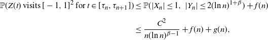 \begin{align*} \mathbb{P}(Z(t)\;\mathrm{ visits }\;[-1,1]^2\;\mathrm{ for }\;t\in[\tau_n,\tau_{n+1}]) & \leq \mathbb{P}(|X_n|\leq1,\,|Y_n|\leq2(\!\ln{n})^{1+\beta}) + f(n) \\[5pt] & \leq \frac{C^2}{n(\!\ln{n})^{\beta-1}} + f(n) + g(n), \end{align*}
where f and g are two summable functions over n, similar to Theorem 3.2. The right-hand side is summable over n as long as
 $\beta>2$
. Hence, Z(t) visits
$\beta>2$
. Hence, Z(t) visits
 $[-1, 1]^2$
finitely often, almost surely.
$[-1, 1]^2$
finitely often, almost surely.
4. Analysis of Model B
Recall that in Model B, the vectors
 $\textbf{f}_n$
are uniformly distributed over the unit sphere in
$\textbf{f}_n$
are uniformly distributed over the unit sphere in
 $\mathbb{R}^d$
.
$\mathbb{R}^d$
.
Throughout this section, we again suppose that
 $\rho=1$
and we show that the process is not 1-recurrent. The proof for general
$\rho=1$
and we show that the process is not 1-recurrent. The proof for general
 $\rho$
is analogous and is omitted.
$\rho$
is analogous and is omitted.
Let
 $W_n=(X_n,Y_n,*,*,\dots,*)$
be the embedded version of the process
$W_n=(X_n,Y_n,*,*,\dots,*)$
be the embedded version of the process
 $Z(t)=(X(t),Y(t),*,*,\dots,*)$
; here,
$Z(t)=(X(t),Y(t),*,*,\dots,*)$
; here,
 $X_n$
and
$X_n$
and
 $Y_n$
(X(t) and Y(t) respectively) stand for the process’ first two coordinates. We denote the projection of Z(t) (
$Y_n$
(X(t) and Y(t) respectively) stand for the process’ first two coordinates. We denote the projection of Z(t) (
 $W_n$
respectively) on the two-dimensional plane by
$W_n$
respectively) on the two-dimensional plane by
 $\hat W(t)=(X(t),Y(t))$
(
$\hat W(t)=(X(t),Y(t))$
(
 $\hat W_n=(X_n,Y_n)$
respectively.) See Figure 2.
$\hat W_n=(X_n,Y_n)$
respectively.) See Figure 2.
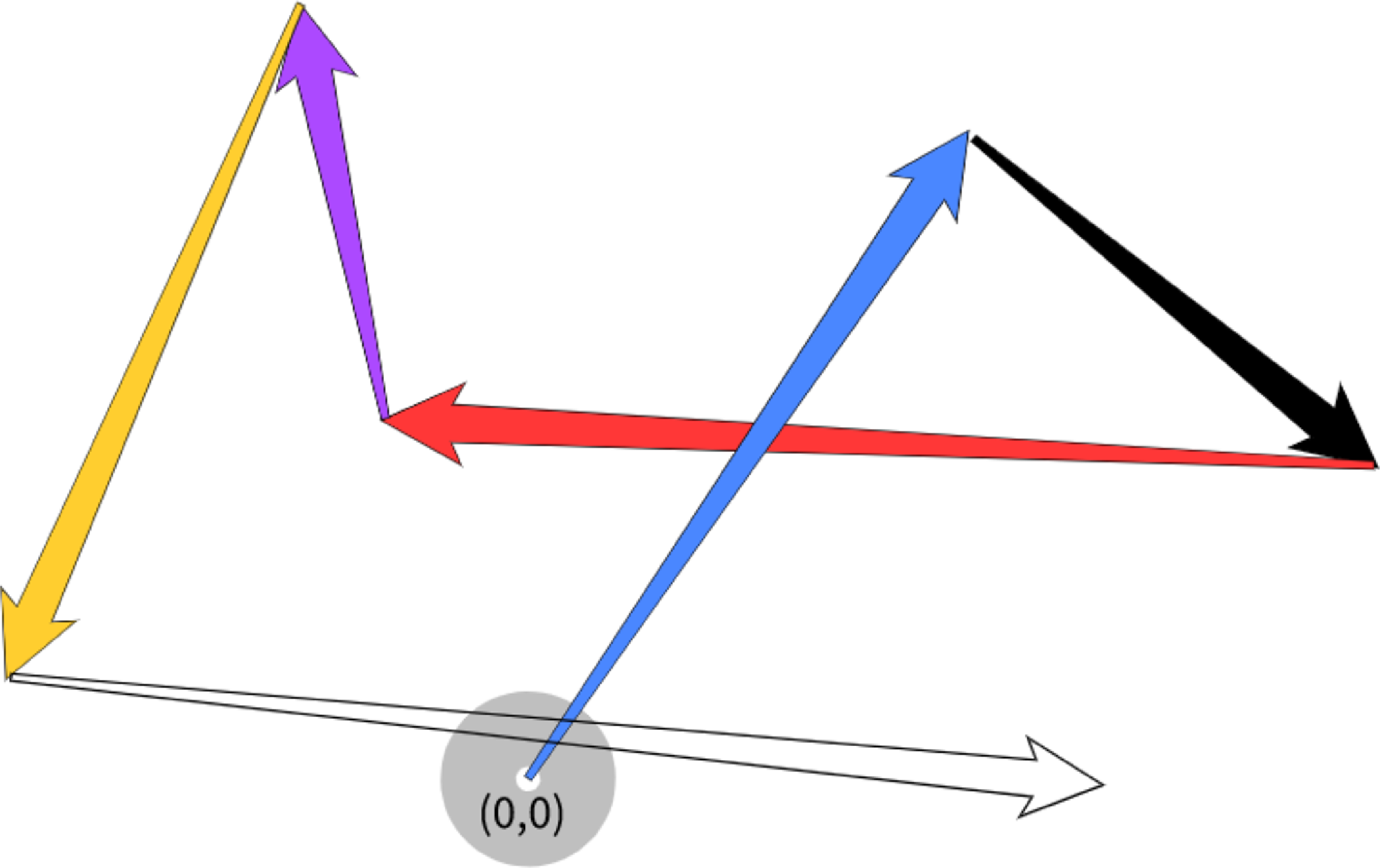
Figure 2. Model B:
 $\hat W_n$
, the (projection of) a conservative random walk on
$\hat W_n$
, the (projection of) a conservative random walk on
 $\mathbb{R}^2$
.
$\mathbb{R}^2$
.
The following statement is quite intuitive.
Lemma 4.1. Suppose
 $d\ge 3$
, and let
$d\ge 3$
, and let
 $\boldsymbol{f}=(f_1,f_2,\dots,f_d)$
be a random vector uniformly distributed on the unit sphere
$\boldsymbol{f}=(f_1,f_2,\dots,f_d)$
be a random vector uniformly distributed on the unit sphere
 $\mathcal{S}^{d-1}$
in
$\mathcal{S}^{d-1}$
in
 $\mathbb{R}^d$
. Then, for some
$\mathbb{R}^d$
. Then, for some
 $\gamma>0$
,
$\gamma>0$
,
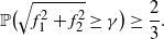 \begin{align*} \mathbb{P}\big(\sqrt{f_1^2+f_2^2}\ge \gamma\big) \ge \frac23. \end{align*}
Remark 4.1. The statement is trivially true for the case
 $d=2$
as well.
$d=2$
as well.
Proof of Lemma
4.1. We use the following well-known representation (see, e.g., [Reference Blum, Hopcroft and Kannan2, Section 2.5]) of
 $\textbf{f}$
:
$\textbf{f}$
:
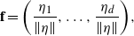 \begin{align*} \textbf{f} = \bigg(\frac{\eta_1}{\Vert\eta\Vert},\dots,\frac{\eta_d}{\Vert\eta\Vert}\bigg), \end{align*}
where
 $\eta_i$
,
$\eta_i$
,
 $i=1,2,\dots$
, are i.i.d. standard normal and
$i=1,2,\dots$
, are i.i.d. standard normal and
 $\Vert\eta\Vert=\sqrt{\eta_1^2+\dots+\eta_d^2}$
. For some large enough
$\Vert\eta\Vert=\sqrt{\eta_1^2+\dots+\eta_d^2}$
. For some large enough
 $A>0$
,
$A>0$
,
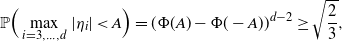 \begin{align*} \mathbb{P}\Big(\max_{i=3,\dots,d}|\eta_i|<A\Big) = (\Phi(A)-\Phi(-A))^{d-2} \ge \sqrt{\frac23}, \end{align*}
where
 $\Phi(\!\cdot\!)$
is the distribution function of the standard normal random variable. Also, for some small enough
$\Phi(\!\cdot\!)$
is the distribution function of the standard normal random variable. Also, for some small enough
 $a\in(0,A)$
,
$a\in(0,A)$
,
 $\mathbb{P}(\max_{i=1,2}|\eta_i|>a)\ge\sqrt{\frac23}$
. On the intersection of these two independent events we have
$\mathbb{P}(\max_{i=1,2}|\eta_i|>a)\ge\sqrt{\frac23}$
. On the intersection of these two independent events we have
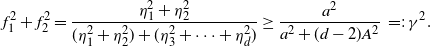 \begin{equation*} f_1^2+f_2^2 = \frac{\eta_1^2+\eta_2^2}{(\eta_1^2+\eta_2^2)+(\eta_3^2+\dots+\eta_d^2)} \ge \frac{a^2}{a^2+(d-2)A^2} \;=\!:\; \gamma^2. \end{equation*}
Remark 4.2. In fact, we can rigorously compute
 \begin{align*} \mathbb{P}(f_1^2+f_2^2\ge \gamma^2) & = \mathbb{P}\bigg(\frac{\eta_1^2+\eta_2^2}{\eta_1^2+\eta_2^2+\dots+\eta_d^2} \ge \gamma^2\bigg) \\[5pt] & = \mathbb{P}\bigg(\eta_1^2+\eta_2^2 \ge \frac{\gamma^2}{1-\gamma^2}(\eta_3^2+\dots+\eta_d^2)\bigg) \\[5pt] & = \mathbb{P}\bigg(\chi^2(2) \ge \frac{\gamma^2}{1-\gamma^2}\chi^2(d-2)\bigg) \\[5pt] & = \iint_{x\ge({\gamma^2}/({1-\gamma^2}))y\ge0}\frac{{\mathrm{e}}^{-x/2}}2 \cdot \frac{y^{d/2-2}{\mathrm{e}}^{-y/2}}{2^{d/2-1}\Gamma(d/2-1)}\,\mathrm{d}x\,\mathrm{d}y \\[5pt] & = \int_0^\infty{\mathrm{e}}^{-({y}/2)\cdot({\gamma^2 }/({2(1-\gamma^2)}))} \cdot \frac{y^{d/2-2}{\mathrm{e}}^{-y/2}}{2^{d/2-1}\Gamma(d/2-1)}\,\mathrm{d}y = (1-\gamma^2)^{d/2-1}; \end{align*}
however, we do not really need this exact expression.
Lemma 4.2. Suppose
 $d\ge 2$
, and let
$d\ge 2$
, and let
 $R_k=\{(x,y)\in\mathbb{R}^2\colon k^2\le x^2+y^2\le (k+1)^2\}$
be the ring of radius k and width 1 centered at the origin. For some constant
$R_k=\{(x,y)\in\mathbb{R}^2\colon k^2\le x^2+y^2\le (k+1)^2\}$
be the ring of radius k and width 1 centered at the origin. For some constant
 $C>0$
, possibly depending on d and
$C>0$
, possibly depending on d and
 $\alpha$
,
$\alpha$
,
 \begin{equation*} \mathbb{P}\big(\hat W_n^{(1)}\in R_k\big) \le \frac{Ck}{n^{1+({2\alpha}/({1-\alpha}))}}, \qquad \mathbb{P}\big(\hat W_n^{(2)}\in R_k\big) \le \frac{Ck}{n(\!\ln{n})^{2\beta}} \end{equation*}
for all large n, where
 $\hat W_t^{(1)}$
is the walk with rate (2.2) and
$\hat W_t^{(1)}$
is the walk with rate (2.2) and
 $\hat W_t^{(2)}$
is the walk with rate (3.8).
$\hat W_t^{(2)}$
is the walk with rate (3.8).
Proof. Assume that the event
 $\mathcal{E}_1$
defined by (3.1) has occurred. We can write
$\mathcal{E}_1$
defined by (3.1) has occurred. We can write
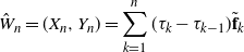 \begin{align*} \hat W_n = (X_n,Y_n) = \sum_{k=1}^n(\tau_k-\tau_{k-1})\tilde{\textbf{f}}_k \end{align*}
where
 $\tilde{\textbf{f}}_k=\ell_k[\textbf{e}_{\textbf{1}}\cos(\phi_k)+\textbf{e}_{\textbf{2}}\sin(\phi_k)]$
,
$\tilde{\textbf{f}}_k=\ell_k[\textbf{e}_{\textbf{1}}\cos(\phi_k)+\textbf{e}_{\textbf{2}}\sin(\phi_k)]$
,
 $\phi_k$
,
$\phi_k$
,
 $k=1,2,\dots$
, are uniformly distributed on
$k=1,2,\dots$
, are uniformly distributed on
 $[\!-\!\pi,\pi]$
, and
$[\!-\!\pi,\pi]$
, and
 $\ell_k$
is the length of the projection
$\ell_k$
is the length of the projection
 $\tilde{\textbf{f}}_k$
of
$\tilde{\textbf{f}}_k$
of
 $\textbf{f}_k$
on the two-dimensional plane. Note that the elements of the set
$\textbf{f}_k$
on the two-dimensional plane. Note that the elements of the set
 $\{\ell_1,\eta_2,\eta_3,\dots,\phi_1,\phi_2,\phi_3,\dots\}$
are all independent. Also, define
$\{\ell_1,\eta_2,\eta_3,\dots,\phi_1,\phi_2,\phi_3,\dots\}$
are all independent. Also, define
 \begin{align*} \mathcal{D}_2 = \{\mathrm{for\;at\;least\;half\;of\;the\;integers }\; i\in[n/2,n]\;\mathrm{ we\;have }\;\ell_i\ge\gamma\}, \end{align*}
where
 $\gamma$
is the constant from Lemma 4.1. Then
$\gamma$
is the constant from Lemma 4.1. Then
 $\mathbb{P}(\mathcal{D}_2^\mathrm{c})\le2{\mathrm{e}}^{-n/36}$
by (2.1) and Lemma 4.1.
$\mathbb{P}(\mathcal{D}_2^\mathrm{c})\le2{\mathrm{e}}^{-n/36}$
by (2.1) and Lemma 4.1.
Let
 $\tilde W_n$
be the distribution of
$\tilde W_n$
be the distribution of
 $\hat W_n\in\mathbb{R}^2$
conditioned on
$\hat W_n\in\mathbb{R}^2$
conditioned on
 $\mathcal{E}_1 \cap \mathcal{D}_2$
, and
$\mathcal{E}_1 \cap \mathcal{D}_2$
, and
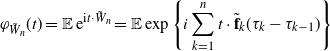 \begin{align*} \varphi_{\tilde W_n}(t) = \mathbb{E}\,{\mathrm{e}}^{\mathrm{i}t\cdot\tilde W_n} = \mathbb{E}\exp\Bigg\{i\sum_{k=1}^n t\cdot\tilde{\textbf{f}}_{k}(\tau_k-\tau_{k-1})\Bigg\} \end{align*}
be its characteristic function (here,
 $t\cdot\tilde{\textbf{f}}_k=\ell_k(t_1\cos(\phi_k)+t_2\sin(\phi_k))$
). We use the Lévy inversion formula, which allows us to compute the density of
$t\cdot\tilde{\textbf{f}}_k=\ell_k(t_1\cos(\phi_k)+t_2\sin(\phi_k))$
). We use the Lévy inversion formula, which allows us to compute the density of
 $\tilde W_n$
, provided
$\tilde W_n$
, provided
 $|\varphi_{\tilde W_n}(t)|$
is integrable:
$|\varphi_{\tilde W_n}(t)|$
is integrable:
 \begin{equation} f_{\tilde W_n}(x,y) = \frac{1}{(2\pi)^2} \iint_{\mathbb{R}^2}{\mathrm{e}}^{-\mathrm{i}(t_1 x+t_2 y)}\varphi_{\tilde W_n}(t)\,\mathrm{d}t_1\,\mathrm{d}t_2 \le \frac{1}{(2\pi)^2}\iint_{\mathbb{R}^2}\big|\varphi_{\tilde W_n}(t)\big|\,\mathrm{d}t_1\,\mathrm{d}t_2. \end{equation}
Let
 $\Delta_k=\tau_k-\tau_{k-1}$
. Since
$\Delta_k=\tau_k-\tau_{k-1}$
. Since
 $\phi_1,\dots,\phi_n$
are i.i.d. Uniform
$\phi_1,\dots,\phi_n$
are i.i.d. Uniform
 $[-\pi,\pi]$
and independent of anything, we have
$[-\pi,\pi]$
and independent of anything, we have
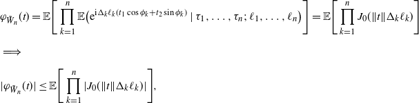 \begin{align*} & \varphi_{\tilde W_n}(t) = \mathbb{E}\Bigg[\prod_{k=1}^n\mathbb{E}\big( {\mathrm{e}}^{\mathrm{i}\Delta_k\ell_k(t_1\cos\phi_k+t_2\sin\phi_k)}\mid\tau_1,\dots,\tau_n;\;\ell_1,\dots,\ell_n\big)\Bigg] = \mathbb{E}\Bigg[\prod_{k=1}^n J_0(\Vert t\Vert\Delta_k\ell_k)\Bigg] \\[5pt] & \Longrightarrow \\[5pt] & |\varphi_{\tilde W_n}(t)| \le \mathbb{E}\Bigg[\prod_{k=1}^n|J_0(\Vert t\Vert \Delta_k\ell_k)|\Bigg], \end{align*}
where
 $\Vert t\Vert=\sqrt{t_1^2+t_2^2}$
, and
$\Vert t\Vert=\sqrt{t_1^2+t_2^2}$
, and
 $J_0(x)=\sum_{m=0}^\infty{(-x^2/4)^{m}}/{m!^2}$
is the Bessel
$J_0(x)=\sum_{m=0}^\infty{(-x^2/4)^{m}}/{m!^2}$
is the Bessel
 $J_0$
function. Indeed, for any
$J_0$
function. Indeed, for any
 $x\in\mathbb{R}$
, setting
$x\in\mathbb{R}$
, setting
 $\tilde x=x\sqrt{t_1^2+t_2^2}$
and
$\tilde x=x\sqrt{t_1^2+t_2^2}$
and
 $\beta=\arctan({t_2}/{t_1})$
, we get
$\beta=\arctan({t_2}/{t_1})$
, we get
 \begin{align*} & \mathbb{E}\big[{\mathrm{e}}^{\mathrm{i}x(t_1\cos\phi_k+t_2\sin\phi_k)}\big] = \frac{1}{2\pi}\int_0^{2\pi}{\mathrm{e}}^{\mathrm{i}x(t_1\cos\phi+t_2\sin\phi)}\,\mathrm{d}\phi = \frac{1}{2\pi}\int_0^{2\pi}{\mathrm{e}}^{\mathrm{i}\tilde x(\cos\beta\cos\phi+\sin\beta\sin\phi)}\, \\[5pt] &\mathrm{d}\phi = \frac{1}{2\pi}\int_0^{2\pi}{\mathrm{e}}^{\mathrm{i}\tilde x\cos(\phi+\beta)}\,\mathrm{d}\phi = \frac{1}{2\pi}\int_0^{2\pi}{\mathrm{e}}^{\mathrm{i}\tilde x\cos(\phi)}\,\mathrm{d}\phi = \frac{1}{2\pi}\int_0^{2\pi}\cos(\tilde x\cos(\phi))\,\mathrm{d}\phi = J_0(\tilde x) \end{align*}
due to periodicity of
 $\cos(\!\cdot\!)$
, the fact that the function
$\cos(\!\cdot\!)$
, the fact that the function
 $\sin(\!\cdot\!)$
is odd, and [Reference Abramowitz and Stegun1, (9.1.18)].
$\sin(\!\cdot\!)$
is odd, and [Reference Abramowitz and Stegun1, (9.1.18)].
Let
 $\xi_k$
be the random variable with the distribution of
$\xi_k$
be the random variable with the distribution of
 $\Delta_k$
given
$\Delta_k$
given
 $\tau_{k-1}$
. Then, recalling that we are on the event
$\tau_{k-1}$
. Then, recalling that we are on the event
 $\mathcal{E}_1$
, we get
$\mathcal{E}_1$
, we get
 $\xi_k\succ\tilde\xi^{(1)}$
for
$\xi_k\succ\tilde\xi^{(1)}$
for
 $\hat{W}^{(1)}_n$
and
$\hat{W}^{(1)}_n$
and
 $\xi_k\succ\tilde\xi^{(2)}$
for
$\xi_k\succ\tilde\xi^{(2)}$
for
 $\hat{W}^{(2)}_n$
, where
$\hat{W}^{(2)}_n$
, where
 $\tilde\xi^{(1)}$
(
$\tilde\xi^{(1)}$
(
 $\tilde\xi^{(2)}$
respectively) is an exponential random variable with rate
$\tilde\xi^{(2)}$
respectively) is an exponential random variable with rate
 $1/{a_1}$
(
$1/{a_1}$
(
 $1/a_2$
respectively) with
$1/a_2$
respectively) with
 $a_1=\tilde c_1 n^{{\alpha}/({1-\alpha})}$
and
$a_1=\tilde c_1 n^{{\alpha}/({1-\alpha})}$
and
 $a_2=\tilde c_2(\!\ln{n})^\beta$
for some constants
$a_2=\tilde c_2(\!\ln{n})^\beta$
for some constants
 $\tilde c_1>0$
and
$\tilde c_1>0$
and
 $\tilde c_2>0$
, and where ‘
$\tilde c_2>0$
, and where ‘
 $\zeta_a\succ\zeta_b$
’ denotes that random variable
$\zeta_a\succ\zeta_b$
’ denotes that random variable
 $\zeta_a$
is stochastically larger than random variable
$\zeta_a$
is stochastically larger than random variable
 $\zeta_b$
. Consequently, setting
$\zeta_b$
. Consequently, setting
 $a=a_1$
,
$a=a_1$
,
 $\tilde\xi=\tilde\xi^{(1)}$
or
$\tilde\xi=\tilde\xi^{(1)}$
or
 $a=a_2$
,
$a=a_2$
,
 $\tilde\xi=\tilde\xi^{(2)}$
, depending on which of the two models we are talking about, and
$\tilde\xi=\tilde\xi^{(2)}$
, depending on which of the two models we are talking about, and
 $\mathcal{F}_k=\sigma(\tau_1,\dots,\tau_k)$
, we get
$\mathcal{F}_k=\sigma(\tau_1,\dots,\tau_k)$
, we get
 \begin{align} \mathbb{E}[|J_0(\Vert t\Vert\Delta_k\ell_k)| \mid \mathcal{F}_{k-1},\ell_k=\ell] & = \mathbb{E}\,|J_0(\Vert t\Vert \xi_k\ell)| \nonumber \\[5pt] & \le \mathbb{E}\,G(\Vert t\Vert\xi_k\ell) \nonumber \\[5pt] & \le \mathbb{E}\,G(\Vert t\Vert\tilde\xi\ell) \nonumber \\[5pt] & = \int_0^\infty a^{-1}{\mathrm{e}}^{-{y}/{a}}G(\Vert t\Vert y\ell)\,\mathrm{d}y \nonumber \\[5pt] & = \int_0^\infty{\mathrm{e}}^{-u}G(su)\,\mathrm{d}u \nonumber \\[5pt] & = \int_0^\infty\frac{{\mathrm{e}}^{-u}}{\sqrt[4]{1+s^2 u^2}\,}\,\mathrm{d}u \;=\!:\; h(s,\ell), \end{align}
where
 $s=a\ell\Vert t\Vert$
, since
$s=a\ell\Vert t\Vert$
, since
 $|J_0(x)|\le G(x)$
by (A.1) and the facts that
$|J_0(x)|\le G(x)$
by (A.1) and the facts that
 $G(\!\cdot\!)$
is a decreasing function and
$G(\!\cdot\!)$
is a decreasing function and
 $\xi_k\succ\tilde\xi$
.
$\xi_k\succ\tilde\xi$
.
We now estimate the function
 $h(t,\ell)$
. Since
$h(t,\ell)$
. Since
 $|J_0(x)|\le 1$
, we trivially get
$|J_0(x)|\le 1$
, we trivially get
 $0\le h(s,\ell)\le 1$
. Additionally, for all
$0\le h(s,\ell)\le 1$
. Additionally, for all
 $s>0$
,
$s>0$
,
 \begin{align*} h(s,\ell) \le \int_{0}^\infty\frac{{\mathrm{e}}^{-u}}{\sqrt{su}\,}\,\mathrm{d}u = \sqrt{\frac{\pi}{s}} = \sqrt{\frac{\pi}{a\ell\Vert t\Vert}}. \end{align*}
Let
 $n/2\le j_1<j_2<\dots<j_m\le n$
be the indices
$n/2\le j_1<j_2<\dots<j_m\le n$
be the indices
 $i\in[n/2,n]$
for which
$i\in[n/2,n]$
for which
 $\ell_i\ge\gamma$
. Since
$\ell_i\ge\gamma$
. Since
 $|J_0(x)|\le 1$
, we have, from (4.2),
$|J_0(x)|\le 1$
, we have, from (4.2),
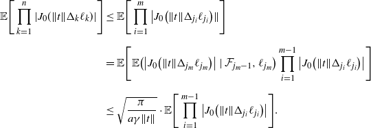 \begin{align*} \mathbb{E}\Bigg[\prod_{k=1}^n|J_0(\Vert t\Vert\Delta_k\ell_k)|\Bigg] & \le \mathbb{E}\Bigg[\prod_{i=1}^m\big|J_0\big(\Vert t\Vert\Delta_{j_i}\ell_{j_i}\big)\|\Bigg] \\[5pt] & = \mathbb{E}\Bigg[\mathbb{E}\big(\big|J_0\big(\Vert t\Vert\Delta_{j_m}\ell_{j_m}\big)\big| \mid \mathcal{F}_{j_m-1},\ell_{j_m}\big) \prod_{i=1}^{m-1}\big|J_0\big(\Vert t\Vert\Delta_{j_i}\ell_{j_i}\big)\big|\Bigg] \\[5pt] & \le \sqrt{\frac{\pi}{a\gamma\Vert t\Vert}} \cdot \mathbb{E}\Bigg[\prod_{i=1}^{m-1}\big|J_0\big(\Vert t\Vert\Delta_{j_i}\ell_{j_i}\big)\big|\Bigg]. \end{align*}
By iterating this argument for
 $i=j_{m-1},j_{m-2},\dots,j_1$
, we get
$i=j_{m-1},j_{m-2},\dots,j_1$
, we get
 \begin{align*} \big|\varphi_{\tilde W_n}(t)\big| \le \mathbb{E}\Bigg[\prod_{k=1}^n|J_0(\Vert t\Vert\Delta_k\ell_k)|\Bigg] \le \bigg(\sqrt{\frac{\pi}{a\gamma\Vert t\Vert}}\bigg)^{n/4} \end{align*}
(recall that
 $m\ge n/4$
on
$m\ge n/4$
on
 $\mathcal{D}_1$
).
$\mathcal{D}_1$
).
Now consider two cases. For
 $\Vert t\Vert\ge\frac{2\pi}{a\gamma}$
, part of the inversion formula gives
$\Vert t\Vert\ge\frac{2\pi}{a\gamma}$
, part of the inversion formula gives
 \begin{align} \iint_{\Vert t\Vert>{2\pi}/{a\gamma}}\big|\varphi_{\tilde W_n}(t)\big|\,\mathrm{d}t_1\,\mathrm{d}t_2 & \le \iint_{\Vert t\Vert\ge{2\pi}/{a\gamma}} \bigg(\frac{\pi}{\gamma\Vert t\Vert a}\bigg)^{n/8}\,\mathrm{d}t_1\,\mathrm{d}t_2 \nonumber \\[5pt] & = \bigg(\frac{\pi}{a\gamma}\bigg)^2\int_0^{2\pi}\,\mathrm{d}\theta\int_2^\infty\frac{r\,\mathrm{d}r}{r^{n/8}} \nonumber \\[5pt] & = \frac{2\pi^3}{a^2\gamma^2}\cdot\frac{r^{2-n/8}}{2-n/8}\bigg|_2^\infty = o(2^{-n/8}) \end{align}
by changing the variables
 $t_1=({\pi}/{a\gamma})r\cos\theta$
,
$t_1=({\pi}/{a\gamma})r\cos\theta$
,
 $t_2=({\pi}/{a\gamma})r\sin\theta$
.
$t_2=({\pi}/{a\gamma})r\sin\theta$
.
On the other hand, for
 $\Vert t\Vert\le{2\pi}/{a\gamma}$
, when
$\Vert t\Vert\le{2\pi}/{a\gamma}$
, when
 $\ell\ge\gamma$
and thus
$\ell\ge\gamma$
and thus
 $\sigma\;:\!=\;a\gamma\Vert t\Vert\le s$
,
$\sigma\;:\!=\;a\gamma\Vert t\Vert\le s$
,
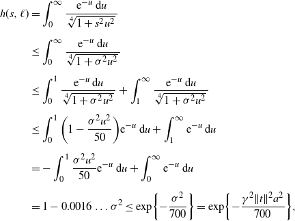 \begin{align*} h(s,\ell) & = \int_0^\infty\frac{{\mathrm{e}}^{-u}\,\mathrm{d}u}{\sqrt[4]{1+s^2u^2}\,} \\[5pt] & \le \int_0^\infty\frac{{\mathrm{e}}^{-u}\,\mathrm{d}u}{\sqrt[4]{1+\sigma ^2u^2}\,} \\[5pt] & \le \int_0^1\frac{{\mathrm{e}}^{-u}\,\mathrm{d}u}{\sqrt[4]{1+\sigma^2u^2}\,} + \int_1^\infty\frac{{\mathrm{e}}^{-u}\,\mathrm{d}u}{\sqrt[4]{1+\sigma^2u^2}\,} \\[5pt] & \le \int_0^1\bigg(1-\frac{\sigma^2u^2}{50}\bigg){\mathrm{e}}^{-u}\,\mathrm{d}u + \int_1^\infty{\mathrm{e}}^{-u}\,\mathrm{d}u \\[5pt] & = -\int_0^1\frac{\sigma^2u^2}{50}{\mathrm{e}}^{-u}\,\mathrm{d}u + \int_{0}^\infty{\mathrm{e}}^{-u}\,\mathrm{d}u \\[5pt] & = 1 - 0.0016\ldots\sigma^2 \le \exp\!\bigg\{{-}\frac{\sigma^2}{700}\bigg\} = \exp\!\bigg\{{-}\frac{\gamma^2\Vert t\Vert^2 a^2}{700}\bigg\}, \end{align*}
since
 $(1+x^2)^{-1/4}\le 1-x^2/50$
for
$(1+x^2)^{-1/4}\le 1-x^2/50$
for
 $0\le x\le 7$
, and
$0\le x\le 7$
, and
 $\sigma\le 2\pi<7$
by assumption. By iterating the same argument as before, we get
$\sigma\le 2\pi<7$
by assumption. By iterating the same argument as before, we get
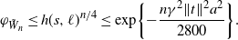 \begin{align*} \varphi_{\tilde W_n} \le h(s,\ell)^{n/4} \le \exp\!\bigg\{{-}\frac{n\gamma^2\Vert t\Vert^2 a^2}{2800}\bigg\}. \end{align*}
Consequently,
 \begin{align} \iint_{\Vert t\Vert\le{2\pi}/{a\gamma}}\big|\varphi_{\tilde W_n}(t)\big|\,\mathrm{d}t_1\,\mathrm{d}t_2 & \le \iint_{\Vert t\Vert\le{2\pi}/{a\gamma}}\exp\!\bigg\{{-}\frac{n\gamma^2\Vert t\Vert^2 a^2}{2800}\bigg\}\, \mathrm{d}t_1\mathrm{d}t_2 \nonumber \\[5pt] & \le \frac{1400}{a^2\gamma^2}\int_0^{2\pi}\mathrm{d}\theta \int_0^\infty\exp\!\bigg\{{-}\frac{nr^2}2\bigg\}r\,\mathrm{d}r = \frac{2800\pi}{na^2\gamma^2} \end{align}
by changing the variables
 $t_1=({10\sqrt{14}}/{a\gamma})r\cos\theta$
,
$t_1=({10\sqrt{14}}/{a\gamma})r\cos\theta$
,
 $t_2=({10\sqrt{14}}/{a\gamma})r\sin\theta$
.
$t_2=({10\sqrt{14}}/{a\gamma})r\sin\theta$
.
Finally, recalling that
 $a_1\sim n^{{\alpha}/({1-\alpha})}$
for
$a_1\sim n^{{\alpha}/({1-\alpha})}$
for
 $\hat W_t^{(1)}$
and
$\hat W_t^{(1)}$
and
 $a_2\sim(\!\ln{n})^\beta$
for
$a_2\sim(\!\ln{n})^\beta$
for
 $\hat W_t^{(2)}$
, from (4.1), (4.3), and (4.4) we obtain
$\hat W_t^{(2)}$
, from (4.1), (4.3), and (4.4) we obtain
 \begin{equation*} f_{\tilde W_n^{(1)}}(x,y) \le O\bigg(\frac{1}{n^{1+({2\alpha}/({1-\alpha}))}}\bigg), \qquad f_{\tilde W_n^{(2)}}(x,y) \le O\bigg(\frac{1}{n(\!\ln{n})^{2\beta}}\bigg). \end{equation*}
Hence,
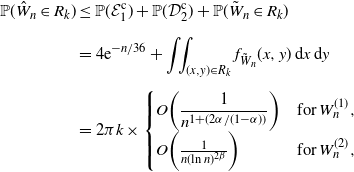 \begin{align*} \mathbb{P}(\hat W_n\in R_k) & \le \mathbb{P}(\mathcal{E}_1^\mathrm{c}) + \mathbb{P}(\mathcal{D}_2^\mathrm{c}) + \mathbb{P}(\tilde W_n\in R_k) \\[5pt] & = 4{\mathrm{e}}^{-n/36} + \iint_{(x,y)\in R_k}f_{\tilde W_n}(x,y)\,\mathrm{d}x\,\mathrm{d}y \\[5pt] & = 2\pi k\times \begin{cases} O\bigg(\dfrac{1}{n^{1+({2\alpha}/({1-\alpha}))}}\bigg) & \mathrm{for }\;W_n^{(1)}, \\[5pt] O\bigg(\frac{1}{n(\!\ln{n})^{2\beta}}\bigg) & \mathrm{for }\;W_n^{(2)}, \end{cases} \end{align*}
since the area of
 $R_k$
is
$R_k$
is
 $\pi(2k+1)$
.
$\pi(2k+1)$
.
Lemma 4.3. Suppose
 $d\ge 2$
and
$d\ge 2$
and
 $\hat W_n=r>1$
. Then
$\hat W_n=r>1$
. Then
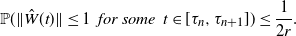 \begin{align*} \mathbb{P}(\Vert\hat W(t)\Vert\le 1\; \textit{ for\;some }\; t\in[\tau_n,\tau_{n+1}]) \le \frac{1}{2r}. \end{align*}
Proof. First, note that
 $\hat W_n$
lies outside the unit circle on
$\hat W_n$
lies outside the unit circle on
 $\mathbb{R}^2$
. The projection
$\mathbb{R}^2$
. The projection
 $\tilde{\textbf{f}}_{n+1}$
of
$\tilde{\textbf{f}}_{n+1}$
of
 $\textbf{f}_{n+1}$
on the first two coordinates’ plane has an angle
$\textbf{f}_{n+1}$
on the first two coordinates’ plane has an angle
 $\phi$
uniformly distributed over
$\phi$
uniformly distributed over
 $[0,2\pi]$
. The probability in the statement of the lemma is monotone increasing in
$[0,2\pi]$
. The probability in the statement of the lemma is monotone increasing in
 $\tau_{n+1}$
, and hence is bounded above by
$\tau_{n+1}$
, and hence is bounded above by
 \begin{align*} \mathbb{P}(\mathrm{the\;infinite\;ray\;from }\;\hat W_n\;\mathrm{ in\;the\;direction }\;\tilde{\textbf{f}}_{n+1} \;\mathrm{ passes\;through\;the\;unit\;circle}) = \frac{2\arcsin(1/r)}{2\pi} \end{align*}
(see Figure 3.) Finally,
 $\arcsin(x)\le {\pi x}/{2}$
for
$\arcsin(x)\le {\pi x}/{2}$
for
 $0\le x\le 1$
.
$0\le x\le 1$
.
Theorem 4.1. Let
 $d\ge 2$
and the walk Z(t) have either the rate (2.2) with
$d\ge 2$
and the walk Z(t) have either the rate (2.2) with
 $\alpha\in(0,1)$
or the rate (3.8) with
$\alpha\in(0,1)$
or the rate (3.8) with
 $\beta>2$
. Then Z(t) is transient a.s.
$\beta>2$
. Then Z(t) is transient a.s.

Figure 3. A ray from
 $\hat W_n$
passes through the unit circle.
$\hat W_n$
passes through the unit circle.
Proof. As mentioned before, we only show that the walk is not
 $\rho$
-recurrent for
$\rho$
-recurrent for
 $\rho=1$
. To do that, it will suffice that, a.s., there will be only finitely many n such that the event
$\rho=1$
. To do that, it will suffice that, a.s., there will be only finitely many n such that the event
 $A_n=\{\Vert\hat{W}(t)\Vert\le1\;\mathrm{ for\;some }\;t\in[\tau_n,\tau_{n+1}]\}$
occurs. Indeed, fix a positive integer n. At this time,
$A_n=\{\Vert\hat{W}(t)\Vert\le1\;\mathrm{ for\;some }\;t\in[\tau_n,\tau_{n+1}]\}$
occurs. Indeed, fix a positive integer n. At this time,
 $\hat W_n\in R_k$
for some
$\hat W_n\in R_k$
for some
 $k\in \{0,1,2,\dots\}$
. According to Lemma 4.3,
$k\in \{0,1,2,\dots\}$
. According to Lemma 4.3,
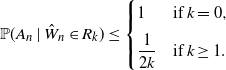 \begin{align*} \mathbb{P}(A_n\mid\hat W_n\in R_k) \le \begin{cases} 1 & \mathrm{if }\; k=0, \\[5pt] \dfrac{1}{2k} & \mathrm{if }\; k\ge 1. \end{cases} \end{align*}
Fix some very small
 $\varepsilon>0$
. Then
$\varepsilon>0$
. Then
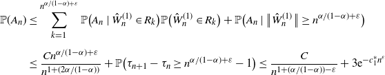 \begin{align*} \mathbb{P}(A_n) & \le \sum_{k=1}^{n^{{\alpha}/({1-\alpha})+\varepsilon}} \mathbb{P}\big(A_n\mid\hat W_n^{(1)}\in R_k\big)\mathbb{P}\big(\hat W_n^{(1)}\in R_k\big) + \mathbb{P}\big(A_n\mid\big\Vert\hat W_n^{(1)}\big\Vert\ge n^{{\alpha}/({1-\alpha})+\varepsilon}\big) \\[5pt] & \le \frac{Cn^{{\alpha}/({1-\alpha})+\varepsilon}}{n^{1+({2\alpha}/({1-\alpha}))}} + \mathbb{P}\big(\tau_{n+1}-\tau_n\ge n^{{\alpha}/({1-\alpha})+\varepsilon}-1\big) \le \frac{C}{n^{1+({\alpha}/({1-\alpha}))-\varepsilon}} + 3{\mathrm{e}}^{-c_1^* n^\varepsilon} \end{align*}
by (3.6) and Lemma 4.2. Hence,
 $\sum_n\mathbb{P}(A_n)<\infty$
and the result follows from the Borel–Cantelli lemma.
$\sum_n\mathbb{P}(A_n)<\infty$
and the result follows from the Borel–Cantelli lemma.
Similarly, in the other case,
 \begin{align*} \mathbb{P}(A_n) & \le \sum_{k=1}^{2(\!\ln{n})^{1+\beta}}\mathbb{P}\big(A_n,\hat W_n^{(2)}\in R_k\big) + \mathbb{P}\big(A_n\mid\big\Vert\hat W_n^{(2)}\big\Vert\ge{2(\!\ln{n})^{1+\beta}}\big) \\[5pt] & \le \frac{2C(\!\ln{n})^{1+\beta}}{n(\!\ln{n})^{2\beta}} + \mathbb{P}(\tau_{n+1}-\tau_n\ge2(\!\ln{n})^{1+\beta}-1) \le \frac{2C}{n(\!\ln{n})^{\beta-1}} + \frac{1}{n^2} \end{align*}
for all sufficiently large n by (3.9) and Lemma 4.2. Hence,
 $\sum_n\mathbb{P}(A_n)<\infty$
for
$\sum_n\mathbb{P}(A_n)<\infty$
for
 $\beta>2$
, and the result again follows from the Borel–Cantelli lemma.
$\beta>2$
, and the result again follows from the Borel–Cantelli lemma.
Appendix A. Properties of the Bessel function
$J_0$

Let
 \begin{align*}J_0(x)=\sum_{m=0}^\infty \frac{(-1)^m\,(x/2)^{2m}}{(m!)^2}\end{align*}
be the Bessel function of the first kind. The following statement might be known, but we could not find it in the literature.
Claim A.1. For all
 $x\ge 0$
,
$x\ge 0$
,
 \begin{align} |J_0(x)| \le \frac{1}{\sqrt[4]{1+x^2}\,} \;=\!:\; G(x). \end{align}
Proof. From [Reference Krasikov15, Theorem 1 and (1)] we get (with
 $\nu=0$
,
$\nu=0$
,
 $\mu=3$
)
$\mu=3$
)
 \begin{equation*} J_0^2(x) \le \frac{4(4x^2-5)}{\pi( (4x^2-3)^{3/2}-3 )}, \quad x \ge 1.13. \end{equation*}
This inequality also implies that
 \begin{align*} |J_0(x)| \le \frac{1}{\sqrt[4]{1+x^2}\,}, \quad x \ge 1.13. \end{align*}
At the same time, for
 $0\le x\le 2$
(using [1, 9.1.14]),
$0\le x\le 2$
(using [1, 9.1.14]),
 \begin{align*} J_0^2(x) = \sum_{k=0}^\infty(-1)^k\frac{(2k)!}{(k!)^4}\bigg(\frac{x}{2}\bigg)^{2k} \le 1 - 2\bigg(\frac{x}{2}\bigg)^2 + \frac32\bigg(\frac{x}{2}\bigg)^4 - \frac59\bigg(\frac{x}{2}\bigg)^6 + \frac{35}{288}\bigg(\frac{x}{2}\bigg)^8, \end{align*}
and at the same time
 \begin{align*} \frac{1}{\sqrt{1+x^2}\,} \ge 1 - 2\bigg(\frac{x}{2}\bigg)^2 + \frac32\bigg(\frac{x}{2}\bigg)^4 - \frac59\bigg(\frac{x}{2}\bigg)^6 + \frac{35}{288}\bigg(\frac{x}{2}\bigg)^8, \end{align*}
yielding (A.1).
Observe as well that
 $0\le G(x)\le 1/\sqrt{x}$
, and that G is a decreasing function for
$0\le G(x)\le 1/\sqrt{x}$
, and that G is a decreasing function for
 $x\ge 0$
; see Figure 4.
$x\ge 0$
; see Figure 4.
Figure 4.
 $|J_0(x)|$
(red) and its upper bound G(x) (blue).
$|J_0(x)|$
(red) and its upper bound G(x) (blue).
Acknowledgements
We would like to thank the associate editor and the referees for their comments, and especially for providing us with relevant references.
Funding information
The research is supported by Swedish Research Council grant VR 2014-5157 and Crafoord Foundation grant 20190667.
Competing interests
There were no competing interests to declare which arose during the preparation or publication process of this article.


 Open access