


1. Introduction and main results
1.1. Introduction
Complex networks are everywhere. Prominent examples include social networks, the Internet, the World Wide Web, transportation networks, etc. In any network, it is of great interest to be able to quantify who is ‘important’ and who is less so. This is what centrality measures aim to do.
There are several well-known centrality measures in networks [Reference Newman38, Chapter 7], such as degree centrality, PageRank centrality, and betweenness centrality. PageRank, first proposed in [Reference Page, Brin, Motwani and Winograd39], can be visualised as the stationary distribution of a random walk with uniform restarts. Betweenness centrality was first defined by Anthonisse [Reference Anthonisse2]. For a survey of centrality measures, see Boldi and Vigna [Reference Boldi and Vigna8] and Borgatti [Reference Borgatti12].
There are many ways in which we can compare the effectiveness of centrality measures. Here, one can think of importance for spreading diseases or information [Reference Wei, Zhao, Liu and Wang42], for being an information bridge between different communities, or for being an important source of information in a network of scientific papers [Reference Senanayake, Piraveenan and Zomaya41].
In this paper, we compare centrality measures by investigating the rate of disintegration of the network by the removal of central vertices. This approach quantifies the notion that a centrality measure is more effective when the network disintegrates more upon the removal of the most central vertices. This work is motivated by the analysis and simulations performed in [Reference Mocanu, Exarchakos and Liotta35], where the number of connected components and the size of the giant were compared after the removal of the most central vertices based on several centrality measures from a simulation perspective.
Central questions. Our key questions are as follows.
-
How will the number of connected components grow with the removal of the most/least central vertices?
-
Does vertex removal with respect to centrality measures preserve the existence of local limits?
-
What are the subcritical and supercritical regimes of the giant component for vertex removals with respect to centrality measure?
-
What is the proportion of vertices in the giant component?
Main innovation of this paper. To answer the above questions, we rely on the theory of local convergence [Reference Aldous and Steele1, Reference Benjamini and Schramm6]; see also [Reference Hofstad23, Chapter 2] for an extensive overview. We show that when considering strictly local centrality measures, i.e. measures that depend on a fixed-radius neighbourhood of a vertex, the number of connected components after the vertex removal procedure converges, and the local limit of the removed graph can be determined in terms of the original local limit. Thus, this answers the first two questions rather generally, assuming local convergence.
It is well known that the giant in a random graph is not determined by its local limit (even though it frequently ‘almost’ is: see [Reference Hofstad22]). While the upper bound on the giant is always equal to the survival probability of the local limit, the matching lower bound can be different. For instance, take two disjoint unions of graphs with the same size and local limit. Then, the survival probability of the local limit remains the same but the proportion of vertices in the largest connected component is reduced by a factor of 2, which is strictly less than the survival probability if it is positive. To give an example where we can prove that the giant of the vertex-removed graph equals the survival probability of its local limit, we restrict our attention to the configuration model with a given degree distribution, and degree centrality. There, we identify the giant of the vertex-removed graph, and also show that the giant is smaller when removing more degree-central vertices.
1.2. Preliminaries
In this section, we define centrality measures and then give an informal introduction to local convergence, as these play a central role in this paper. We will assume that
 $|V(G)|=n$
, and for convenience assume that
$|V(G)|=n$
, and for convenience assume that
 $V(G)=\{1, \ldots, n\}\equiv[n]$
.
$V(G)=\{1, \ldots, n\}\equiv[n]$
.
1.2.1. Centrality measures
In this section, we define centrality measures.
Definition 1.1. (Centrality measures in undirected graphs.) For a finite (undirected) graph
 $G=(V(G),E(G))$
, a centrality measure is a function
$G=(V(G),E(G))$
, a centrality measure is a function
 $R\colon V(G) \to \mathbb{R}_{\geq0}$
, where we consider v to be central if R(v) is large.
$R\colon V(G) \to \mathbb{R}_{\geq0}$
, where we consider v to be central if R(v) is large.
Centrality measures can be extended to directed graphs, but in this paper we restrict to undirected graphs as in [Reference Mocanu, Exarchakos and Liotta35]. Commonly used examples of centrality measures are as follows.
Degree centrality. In degree centrality, we rank the vertices according to their degrees and then divide the rank by the total number of vertices. We randomly assign ranks to vertices with the same degree, to remove ties.
PageRank centrality. PageRank is a popularly known algorithm for measuring centrality in the World Wide Web [Reference Brin and Page13].
Definition 1.2. (PageRank centrality.) Consider a finite (undirected) graph G. Let
 $e_{j,i}$
be the number of edges between j and i. Denote the degree of vertex
$e_{j,i}$
be the number of edges between j and i. Denote the degree of vertex
 $i \in [n]$
by
$i \in [n]$
by
 $d_{i}$
. Fix a damping factor or teleportation parameter
$d_{i}$
. Fix a damping factor or teleportation parameter
 $c\in(0, 1)$
. Then PageRank is the unique probability vector
$c\in(0, 1)$
. Then PageRank is the unique probability vector
 $\boldsymbol{\pi}_n = (\pi_n(i))_{i\in [n]}$
that satisfies that, for every
$\boldsymbol{\pi}_n = (\pi_n(i))_{i\in [n]}$
that satisfies that, for every
 $i \in [n]$
,
$i \in [n]$
,
 \begin{equation*} \pi_n(i) = c\sum_{j\in [n]}\dfrac{e_{j,i}}{d_j}\pi_n(j) + \dfrac{1-c}{n}, \quad i\in [n].\end{equation*}
Suppose
 $\textbf{1} = (1, 1, \ldots, 1)$
is the all-one vector. Then, with
$\textbf{1} = (1, 1, \ldots, 1)$
is the all-one vector. Then, with
 $P = (p_{i,j})_{i, j \in V(G)}$
and
$P = (p_{i,j})_{i, j \in V(G)}$
and
 $p_{i,j}= e_{i, j}/d_i$
the transition matrix for the random walk on G,
$p_{i,j}= e_{i, j}/d_i$
the transition matrix for the random walk on G,
 \begin{equation} \boldsymbol{\pi}_n = \biggl(\dfrac{1-c}{n}\biggr) \textbf{1}(I-cP)^{-1}. \end{equation}
In order to use local convergence techniques [Reference Garavaglia, Hofstad and Litvak19], it is useful to work with the graph-normalised PageRank, given by
 \begin{equation*} \boldsymbol{R}_n = n\boldsymbol{\pi}_n, \quad\text{for which} \ \dfrac{1}{n}\sum_{j\in [n]}R_n(j) = 1. \end{equation*}
Since
 $c\in(0,1)$
, (1.1) implies
$c\in(0,1)$
, (1.1) implies
 \begin{equation} \boldsymbol{\pi}_n =\biggl( \dfrac{1-c}{n} \biggr) \textbf{1}\sum_{k= 0}^{\infty} c^k P^k. \end{equation}
Equation (1.2) is sometimes called power-iteration for PageRank [Reference Avrachenkov and Lebedev3, Reference Bianchini, Gori and Scarselli7, Reference Boldi, Santini and Vigna9]. It will also be useful to consider the finite-radius PageRank,
 $\boldsymbol{R}_n^{\scriptscriptstyle(N)}$
, for
$\boldsymbol{R}_n^{\scriptscriptstyle(N)}$
, for
 $N\in \mathbb{N}$
, defined by
$N\in \mathbb{N}$
, defined by
 \begin{equation} \boldsymbol{R}_n^{\scriptscriptstyle(N)} \;:\!=\; \biggl( \dfrac{1-c}{n}\biggr) \textbf{1}\sum_{k= 0}^{N} c^k P^k, \end{equation}
which approximates PageRank by a finite number of powers in (1.2). PageRank has been intensely studied on various random graph models [Reference Banerjee and Olvera-Cravioto5, Reference Chen, Litvak and Olvera-Cravioto15, Reference Chen, Litvak and Olvera-Cravioto16, Reference Garavaglia, Hofstad and Litvak19, Reference Jelenković and Olvera-Cravioto31, Reference Lee and Olvera-Cravioto32, Reference Litvak, Scheinhardt and Volkovich34], with the main focus being to prove or disprove that PageRank has the same power-law exponent as the in-degree distribution.
Other popular centrality measures. Closeness centrality measures the average distance of a vertex from a randomly chosen vertex. The higher the average, the lower the centrality index, and vice versa. Interestingly, Evans and Chen [Reference Evans and Chen18] predict that closeness centrality is closely related to degree centrality, at least for locally tree-like graphs. Betweenness centrality measures the extent to which vertices are important for interconnecting different vertices, and is given by
 \begin{equation*} b_v =\sum_{u\neq v \neq w}\dfrac{\sigma_{u,v}(w)}{\sigma_{u, w}},\end{equation*}
where
 $\sigma_{u, v}$
is the number of shortest paths from vertex u to vertex v, and
$\sigma_{u, v}$
is the number of shortest paths from vertex u to vertex v, and
 $\sigma_{u, v}(w)$
is the number of shortest paths between u and v containing w.
$\sigma_{u, v}(w)$
is the number of shortest paths between u and v containing w.
In this paper we mainly work with strictly local centrality measures.
Definition 1.3. (Strictly local centrality measures.) For a finite (undirected) graph
 $G=(V(G),E(G))$
, a strictly local centrality measure is a centrality measure
$G=(V(G),E(G))$
, a strictly local centrality measure is a centrality measure
 $R \colon V(G) \to \mathbb{R}_{\geq0}$
, such that there exists an
$R \colon V(G) \to \mathbb{R}_{\geq0}$
, such that there exists an
 $r\in \mathbb{N}$
, and for each vertex
$r\in \mathbb{N}$
, and for each vertex
 $v\in V(G)$
, R(v) depends only on the graph through the neighbourhood
$v\in V(G)$
, R(v) depends only on the graph through the neighbourhood
 \begin{equation*} B_{r}^{\scriptscriptstyle(G)}(v) \;:\!=\; \{ u \in V(G)\colon \textrm{dist}_{\scriptscriptstyle G}(u,v) \leq r\}, \end{equation*}
where
 $\textrm{dist}_{\scriptscriptstyle G}(u,v)$
denotes the graph distance between u and v in G.
$\textrm{dist}_{\scriptscriptstyle G}(u,v)$
denotes the graph distance between u and v in G.
PageRank is very well approximated by its strictly local version as in (1.3) [Reference Avrachenkov, Litvak, Nemirovsky and Osipova4, Reference Boldi and Vigna8, Reference Garavaglia, Hofstad and Litvak19].
1.2.2. Local convergence of undirected random graphs
In this section, we informally introduce local convergence of random graphs, which describes what a graph locally looks like from the perspective of a uniformly chosen vertex, as the number of vertices in a graph goes to infinity. For example, the sparse Erdős–Rényi random graph, which is formed by bond-percolation on the complete graph, locally looks like a Poisson branching process, as n tends to infinity [Reference Hofstad23, Chapter 2]. Before moving further, we discuss the following notation.
Notation 1.1. (Probability convergence.) Suppose
 $(X_n)_{n\geq 1}$
,
$(X_n)_{n\geq 1}$
,
 $(Y_n)_{n\geq 1}$
are two sequences of random variables and X is a random variable.
$(Y_n)_{n\geq 1}$
are two sequences of random variables and X is a random variable.
-
(1) We write
 $X_n \overset{\scriptscriptstyle{\mathbb{P}}/d}{\to} X$
when
$X_n$
converges in probability/distribution to X.
$X_n \overset{\scriptscriptstyle{\mathbb{P}}/d}{\to} X$
when
$X_n$
converges in probability/distribution to X. -
(2) We write
$X_n = o_{\scriptscriptstyle\mathbb{P}}(Y_n)$
when
$X_n/Y_n \overset{\scriptscriptstyle\mathbb{P}}{\to} 0$
.


Now let us give the informal definition of local convergence. We will rely on two types of local convergence, namely, local weak convergence and local convergence in probability. Let
 $o_n$
denote a uniformly chosen vertex from
$o_n$
denote a uniformly chosen vertex from
 $V(G_n)$
. Local weak convergence means that
$V(G_n)$
. Local weak convergence means that
 \begin{equation} \mathbb{P}\bigl({B_r^{\scriptscriptstyle(G_n)}(o_n)\cong (H, o')}\bigr) \to \bar{\mu}\bigl(B_r^{\scriptscriptstyle(\bar{G})}(o)\cong (H,o')\bigr),\end{equation}
for all rooted graphs (H, o′), where a rooted graph is a graph with a distinguished vertex in the vertex set V(H) of H. In (1.4),
 $(\bar{G}, o) \sim \bar{\mu}$
is a random rooted graph, which is called the local weak limit. For local convergence in probability, instead, we require that
$(\bar{G}, o) \sim \bar{\mu}$
is a random rooted graph, which is called the local weak limit. For local convergence in probability, instead, we require that
holds for all rooted graphs (H, o′). In (1.5),
 $(G, o) \sim \mu$
is a random rooted graph which is called the local limit in probability (and bear in mind that
$(G, o) \sim \mu$
is a random rooted graph which is called the local limit in probability (and bear in mind that
 $\mu$
can possibly be a random measure on rooted graphs). Both (1.4) and (1.5) describe the convergence of the proportions of vertices around which the graph locally looks like a certain specific graph. We discuss this definition more formally in Section 2.1. We now turn to our main results.
$\mu$
can possibly be a random measure on rooted graphs). Both (1.4) and (1.5) describe the convergence of the proportions of vertices around which the graph locally looks like a certain specific graph. We discuss this definition more formally in Section 2.1. We now turn to our main results.
1.3. Main results
In this section, we state our main results. In Section 1.3.1 we discuss our results that hold for general strictly local centrality measures on locally converging random graph sequences. In Section 1.3.2 we investigate the size of the giant after vertex removal. Due to the non-local nature of the giant, there we restrict to degree centrality on the configuration model.
1.3.1. Strictly local centrality measures
We first define our vertex removal procedure based on centrality.
Definition 1.4. (Vertex removal based on centrality threshold.) Let G be an arbitrary graph. Define G(R, r) to be the graph obtained after removing all the vertices v for which
 $R(v)> r$
. We call this the
$R(v)> r$
. We call this the
 $r$
-killed graph of G.
$r$
-killed graph of G.
Theorem 1.1. (Continuity of vertex removal.) Let R be a strictly local centrality measure and
 ${(G_n)}_{n\geq 1}$
a sequence of random graphs that converges locally weakly/locally in probability to
${(G_n)}_{n\geq 1}$
a sequence of random graphs that converges locally weakly/locally in probability to
 $(G, o) \sim \mu$
. Then
$(G, o) \sim \mu$
. Then
 $(G_n(R, r))_{n\geq 1}$
converges locally weakly/locally in probability to
$(G_n(R, r))_{n\geq 1}$
converges locally weakly/locally in probability to
 $(G(R, r), o)$
, respectively.
$(G(R, r), o)$
, respectively.
Remark 1.1. (Extension to ‘almost’ local centrality measures.) We believe that the proof for Theorem 1.1 can be extended to ‘almost’ local centrality measures like PageRank, but the proof is much more involved.
Theorem 1.1 means that vertex removal with respect to a strictly local centrality threshold is continuous with respect to the local convergence.
Let
 $C_r(o)$
denote the connected component containing the root in the r-killed graph,
$C_r(o)$
denote the connected component containing the root in the r-killed graph,
 $(G(R,r), o)\sim \mu$
. As a corollary to Theorem 1.1, we bound the limiting value of the proportion of vertices in the giant component in
$(G(R,r), o)\sim \mu$
. As a corollary to Theorem 1.1, we bound the limiting value of the proportion of vertices in the giant component in
 $G_n(R, r)$
in probability by the survival probability of
$G_n(R, r)$
in probability by the survival probability of
 $(G(R, r), o)\sim \mu$
, which is
$(G(R, r), o)\sim \mu$
, which is
 $\mu(|C_r(o)| = \infty)$
.
$\mu(|C_r(o)| = \infty)$
.
Corollary 1.1. (Upper bound on giant.) Let
 $v(C_1(G_n(R, r))$
denote the number of vertices in the giant component of
$v(C_1(G_n(R, r))$
denote the number of vertices in the giant component of
 $G_n(R, r)$
. Under the conditions of Theorem 1.1,
$G_n(R, r)$
. Under the conditions of Theorem 1.1,
 \begin{align*}\lim_{n\to \infty}\mathbb{P}(v(C_1(G_n(R, r)))\leq n(\zeta + \varepsilon)) = 1, \end{align*}
for all
 $\varepsilon>0$
, where
$\varepsilon>0$
, where
 $\zeta = \mu(|C_r(o)| = \infty).$
The intuition for Corollary 1.1 is as follows. For any integer k, the set of vertices with component sizes larger than k, if non-empty, contains the vertices in the largest connected component. Thus the proportion of vertices with component size larger than k is an upper bound for the proportion of vertices in the giant component. The former, when divided by n, is the probability that a uniformly chosen vertex has a component size greater than k, which converges due to local convergence properties of the graph sequence. Sending k to infinity gives us the required upper bound.
Let
 $K_n^r(R)$
denote the number of connected component in the killed graph
$K_n^r(R)$
denote the number of connected component in the killed graph
 $G_n(R, r)$
. As another corollary to Theorem 1.1, we give the convergence properties for
$G_n(R, r)$
. As another corollary to Theorem 1.1, we give the convergence properties for
 $K_n^r(R)$
.
$K_n^r(R)$
.
Corollary 1.2. (Number of connected components.) Under the conditions of Theorem 1.1, we have the following.
-
(a) If
${(G_n)}_{n\geq 1}$
converges locally in probability to
$(G, o) \sim \mu$
, then
\begin{equation*} \dfrac{K_n^r(R)}{n} \overset{\scriptscriptstyle\mathbb{P}}{\to} \mathbb{E}_{\mu}\biggl[\dfrac{1}{|C_r(o)|}\biggr]. \end{equation*}
-
(b) If
${(G_n)}_{n\geq 1}$
converges locally weakly to
$(\bar{G}, \bar{o}) \sim \bar{\mu}$
, then
\begin{equation*} \dfrac{\mathbb{E}[K_n^r(R)]}{n} \to \mathbb{E}_{\bar{\mu}}\biggl[\dfrac{1}{|C_r(o)|}\biggr]. \end{equation*}


The limit in Corollary 1.2 follows from the identity
 \begin{equation*} \dfrac{K_n}{n} = \dfrac{1}{n}\sum_{v\in V(G)}\dfrac{1}{|C(v)|}= \mathbb{E}_n\biggl[\dfrac{1}{|C(o_n)|}\biggr],\end{equation*}
where
 $o_n$
is a uniformly chosen vertex and
$o_n$
is a uniformly chosen vertex and
 $|C(v)|$
is the connected component containing v. The function
$|C(v)|$
is the connected component containing v. The function
 $f(G, v) = 1/|C(v)|$
is continuous and bounded on the metric space of rooted graphs. Thus we can apply local convergence results on this function.
$f(G, v) = 1/|C(v)|$
is continuous and bounded on the metric space of rooted graphs. Thus we can apply local convergence results on this function.
1.3.2. Degree centrality and configuration model
In this section, we restrict to degree centrality in the configuration model. Before starting with our main results, we introduce the configuration model.
Configuration model. The configuration model was introduced by Bollobás [Reference Bollobás10]; see also [Reference Hofstad21, Chapter 7] and the references therein for an extensive introduction. It is one of the simplest possible models for generating a random graph with a given degree distribution. Written as
 $\textrm{CM}_n(\boldsymbol{d})$
, it is a random graph on n vertices having a given degree sequence
$\textrm{CM}_n(\boldsymbol{d})$
, it is a random graph on n vertices having a given degree sequence
 $\boldsymbol{d}$
, where
$\boldsymbol{d}$
, where
 $\boldsymbol{d} = (d_1, d_2,\ldots, d_n) \in\mathbb{N}^{n}.$
The giant in the configuration model has attracted considerable attention in, for example, [Reference Bollobás and Riordan11], [Reference Hofstad22], [Reference Janson and Luczak30], [Reference Molloy and Reed36], and [Reference Molloy and Reed37]. It is also known how the tail of the limiting degree distribution influences the size of giant [Reference Deijfen, Rosengren and Trapman17]. Further, the diameter and distances in the supercritical regime have been studied in [Reference Hofstad, Hooghiemstra and Van Mieghem24], [Reference Hofstad, Hooghiemstra and Znamenski25], and [Reference Hofstad, Hooghiemstra and Znamenski26], while criteria for the graph to be simple appear in [Reference Britton, Deijfen and Martin-Löf14], [Reference Janson28], and [Reference Janson29]. In this paper we assume that the degrees satisfy the following usual conditions.
$\boldsymbol{d} = (d_1, d_2,\ldots, d_n) \in\mathbb{N}^{n}.$
The giant in the configuration model has attracted considerable attention in, for example, [Reference Bollobás and Riordan11], [Reference Hofstad22], [Reference Janson and Luczak30], [Reference Molloy and Reed36], and [Reference Molloy and Reed37]. It is also known how the tail of the limiting degree distribution influences the size of giant [Reference Deijfen, Rosengren and Trapman17]. Further, the diameter and distances in the supercritical regime have been studied in [Reference Hofstad, Hooghiemstra and Van Mieghem24], [Reference Hofstad, Hooghiemstra and Znamenski25], and [Reference Hofstad, Hooghiemstra and Znamenski26], while criteria for the graph to be simple appear in [Reference Britton, Deijfen and Martin-Löf14], [Reference Janson28], and [Reference Janson29]. In this paper we assume that the degrees satisfy the following usual conditions.
Condition 1.1. (Degree conditions.) Let
 $\boldsymbol{d} = (d_1, d_2, \ldots , d_n)$
denote a degree sequence. Let
$\boldsymbol{d} = (d_1, d_2, \ldots , d_n)$
denote a degree sequence. Let
 $n_j=\{v\colon d_v=j\}$
denote the number of vertices with degree j. We assume that there exists a probability distribution
$n_j=\{v\colon d_v=j\}$
denote the number of vertices with degree j. We assume that there exists a probability distribution
 $(p_j)_{j\geq 1}$
such that the following hold:
$(p_j)_{j\geq 1}$
such that the following hold:
-
(a)
$\lim_{n\rightarrow \infty}n_j/n= p_j$
, -
(b)
$\lim_{n\rightarrow \infty}\sum_{j\geq 1} j n_j/n= \sum_{j\geq 1} jp_j<\infty$
.


Let D be a non-negative integer random variable with probability mass function
 $(p_j)_{j\geq 1}$
. These regularity conditions ensure that the sequence of graphs converges locally in probability to a unimodular branching process, with degree distribution D. See [Reference Hofstad23, Chapter 4] for more details.
$(p_j)_{j\geq 1}$
. These regularity conditions ensure that the sequence of graphs converges locally in probability to a unimodular branching process, with degree distribution D. See [Reference Hofstad23, Chapter 4] for more details.
Generalised vertex removal based on degrees. We wish to study the effect of the removal of the
 $\alpha$
proportion of vertices with the highest or lowest degrees on the giant of the configuration model. For this, we define
$\alpha$
proportion of vertices with the highest or lowest degrees on the giant of the configuration model. For this, we define
 $\alpha$
-sequences with respect to a probability mass function as follows.
$\alpha$
-sequences with respect to a probability mass function as follows.
Definition 1.5. (
 $\alpha$
-sequence.) Fix
$\alpha$
-sequence.) Fix
 $\alpha \in (0,1)$
. Let
$\alpha \in (0,1)$
. Let
 $\boldsymbol{r}\;:\!=\; (r_i)_{i\geq1}$
be a sequence of elements of [0, 1] satisfying
$\boldsymbol{r}\;:\!=\; (r_i)_{i\geq1}$
be a sequence of elements of [0, 1] satisfying
 \begin{equation*} \mathbb{E}[r_D] \;:\!=\; \sum_{i\geq1}p_ir_i = \alpha.\end{equation*}
Then
 $\boldsymbol{r}$
is called an
$\boldsymbol{r}$
is called an
 $\alpha$
-sequence with respect to
$\alpha$
-sequence with respect to
 $\boldsymbol{p} = (p_j)_{j\geq 1}$
.
$\boldsymbol{p} = (p_j)_{j\geq 1}$
.
Suppose
 $(G_n)_{n\geq 1}$
is a sequence of random graphs converging locally in probability to
$(G_n)_{n\geq 1}$
is a sequence of random graphs converging locally in probability to
 $(G,o)\sim\mu$
, and let the limiting degree distribution be D, with probability mass function as
$(G,o)\sim\mu$
, and let the limiting degree distribution be D, with probability mass function as
 $\boldsymbol{p} = (p_j)_{j\geq 1}$
. Suppose
$\boldsymbol{p} = (p_j)_{j\geq 1}$
. Suppose
 $\boldsymbol{r}=(r_j)_{j\geq 1}$
is an
$\boldsymbol{r}=(r_j)_{j\geq 1}$
is an
 $\alpha$
-sequence with respect to
$\alpha$
-sequence with respect to
 $\boldsymbol{p}$
; then we define vertex removal based on
$\boldsymbol{p}$
; then we define vertex removal based on
 $\alpha$
-sequences as follows.
$\alpha$
-sequences as follows.
Definition 1.6. (Vertex removal based on
 $\alpha$
-sequences.) Remove
$\alpha$
-sequences.) Remove
 $\lfloor n r_i p_i\rfloor$
vertices of degree i from
$\lfloor n r_i p_i\rfloor$
vertices of degree i from
 $G_n$
uniformly at random, for each
$G_n$
uniformly at random, for each
 $n\geq 1$
. This gives us the vertex-removed graph according to the
$n\geq 1$
. This gives us the vertex-removed graph according to the
 $\alpha$
-sequence
$\alpha$
-sequence
 $\boldsymbol{r}=(r_j)_{j\geq 1}$
, denoted by
$\boldsymbol{r}=(r_j)_{j\geq 1}$
, denoted by
 $(G_{n,\boldsymbol{r}})_{n\geq 1}$
.
$(G_{n,\boldsymbol{r}})_{n\geq 1}$
.
Remark 1.2. In
 $G_{n, \boldsymbol{r}}$
, we asymptotically remove an
$G_{n, \boldsymbol{r}}$
, we asymptotically remove an
 $\alpha$
proportion of vertices because, due to Condition 1.1 and the dominated convergence theorem,
$\alpha$
proportion of vertices because, due to Condition 1.1 and the dominated convergence theorem,
 \begin{equation*} \lim_{n\to \infty}\sum_{j\geq 1}r_j \dfrac{n_j}{n} = \sum_{j\geq 1}r_j p_j = \alpha. \end{equation*}
Results for the configuration model. Let
 $(G_n)_{n\geq1}$
be a sequence of random graphs satisfying
$(G_n)_{n\geq1}$
be a sequence of random graphs satisfying
 $G_n \sim \textrm{CM}_n(\boldsymbol{d})$
. Throughout the paper, we shall assume that
$G_n \sim \textrm{CM}_n(\boldsymbol{d})$
. Throughout the paper, we shall assume that
 \begin{align*}\nu \;:\!=\; \dfrac{\mathbb{E}[D(D-1)]}{\mathbb{E}[D]}>1.\end{align*}
Indeed, for
 $\nu < 1$
, we already know that there is no giant to start with, and it cannot appear by removing vertices.
$\nu < 1$
, we already know that there is no giant to start with, and it cannot appear by removing vertices.
Definition 1.7. (
 $\boldsymbol{r}$
-set.) Suppose
$\boldsymbol{r}$
-set.) Suppose
 $\boldsymbol{r} = (r_j)_{j\geq 1}$
is an
$\boldsymbol{r} = (r_j)_{j\geq 1}$
is an
 $\alpha$
-sequence with respect to
$\alpha$
-sequence with respect to
 $\boldsymbol{p} = (p_j)_{j\geq 1}$
. Let
$\boldsymbol{p} = (p_j)_{j\geq 1}$
. Let
 $X = [0, 1]^{\mathbb{N}}$
be the set of all sequences in [0, 1]. Define the set
$X = [0, 1]^{\mathbb{N}}$
be the set of all sequences in [0, 1]. Define the set
 \begin{align*} S(\boldsymbol{r}) = \Bigl\{({\boldsymbol{r}^{\scriptscriptstyle(\boldsymbol{n})}})_{n\geq 1} \in X^{\mathbb{N}}\colon \lim_{n\to \infty}r_i^{\scriptscriptstyle(n)} = r_i \ \forall i\geq 1\Bigr\}. \end{align*}
An
 $\boldsymbol{r}$
-set
$\boldsymbol{r}$
-set
 $S(\boldsymbol{r})$
can be thought of as the set of those sequences in
$S(\boldsymbol{r})$
can be thought of as the set of those sequences in
 $[0, 1]^{\mathbb{N}}$
which converge to
$[0, 1]^{\mathbb{N}}$
which converge to
 $\boldsymbol{r}$
component-wise. Let
$\boldsymbol{r}$
component-wise. Let
 $v(C_1({\boldsymbol{r}}))$
and
$v(C_1({\boldsymbol{r}}))$
and
 $e(C_1({\boldsymbol{r}}))$
denote the number of vertices and edges in the giant component of
$e(C_1({\boldsymbol{r}}))$
denote the number of vertices and edges in the giant component of
 $G_{n,{\boldsymbol{r}}}$
. The following theorem describes the giant in
$G_{n,{\boldsymbol{r}}}$
. The following theorem describes the giant in
 $G_{n,{\boldsymbol{r}}^{\scriptscriptstyle(\boldsymbol{n})}}$
.
$G_{n,{\boldsymbol{r}}^{\scriptscriptstyle(\boldsymbol{n})}}$
.
Theorem 1.2. (Existence of giant after vertex removal.) Let
 $\boldsymbol{r}$
be an
$\boldsymbol{r}$
be an
 $\alpha$
-sequence. Let
$\alpha$
-sequence. Let
 $(\boldsymbol{r}^{\scriptscriptstyle(n)})_{n\geq 1}$
be a sequence from the
$(\boldsymbol{r}^{\scriptscriptstyle(n)})_{n\geq 1}$
be a sequence from the
 $\boldsymbol{r}$
-set
$\boldsymbol{r}$
-set
 $S(\boldsymbol{r})$
. Then the graph
$S(\boldsymbol{r})$
. Then the graph
 $G_{n,\boldsymbol{r}^{\scriptscriptstyle(n)}}$
has a giant component if and only if
$G_{n,\boldsymbol{r}^{\scriptscriptstyle(n)}}$
has a giant component if and only if
 $\nu_{\boldsymbol{r}}>1$
, where
$\nu_{\boldsymbol{r}}>1$
, where
 \begin{equation} \nu_{\boldsymbol{r}} \;:\!=\; \dfrac{\mathbb{E}[D(D-1)(1-r_D)]}{\mathbb{E}[D]}.\end{equation}
For
 $\nu_{\boldsymbol{r}}>1$
,
$\nu_{\boldsymbol{r}}>1$
,
 \begin{align} \dfrac{v(C_1(\boldsymbol{r}^{\scriptscriptstyle(n)}))}{n}\overset{\scriptscriptstyle\mathbb{P}}{\to}\rho(\boldsymbol{r}) &\;:\!=\; 1- \alpha -2\mathbb{E}[Dr_D]\eta_{\boldsymbol{r}}-\sum_{i\geq 1}(1-r_i)p_i{\eta^i_{\boldsymbol{r}}}, \end{align}
 \begin{align} \dfrac{e(C_1(\boldsymbol{r}^{\scriptscriptstyle(n)}))}{n}\overset{\scriptscriptstyle\mathbb{P}}{\to}e(\boldsymbol{r})&\;:\!=\; \dfrac{\mathbb{E}[D]}{2}(1-{\eta}_{\boldsymbol{r}}^{2})-\mathbb{E}[D r_D](1-{\eta_{\boldsymbol{r}}}) .\end{align}
In the above equations,
 ${\eta_{\boldsymbol{r}}} \in (0, 1]$
is the smallest solution of
${\eta_{\boldsymbol{r}}} \in (0, 1]$
is the smallest solution of
 \begin{equation} g'_{\!\!\boldsymbol{r}}({\eta_{\boldsymbol{r}}}) = \dfrac{\mathbb{E}[D]}{\beta_{\boldsymbol{r}}} {\eta_{\boldsymbol{r}}},\end{equation}
where
 $\beta_{\boldsymbol{r}} = \mathbb{E}[Dr_D]+1-\alpha$
and
$\beta_{\boldsymbol{r}} = \mathbb{E}[Dr_D]+1-\alpha$
and
 $g_{\boldsymbol{r}}(\!\cdot\!)$
is the generating function for a random variable dependent on
$g_{\boldsymbol{r}}(\!\cdot\!)$
is the generating function for a random variable dependent on
 $\boldsymbol{r}$
given by
$\boldsymbol{r}$
given by
 \begin{equation} g_{\boldsymbol{r}}(s) =\dfrac{\sum_{i=1}^{\infty}(1-r_i)p_is^i + \mathbb{E}[Dr_D]s}{\beta_{\boldsymbol{r}}}.\end{equation}
Remark 1.3. (Class of sequences with the same limiting proportion.) For the class of sequences which converge to a given
 $\alpha$
-sequence component-wise, we always have the same limiting proportion of vertices/edges in the giant component. Thus, choosing our sequence
$\alpha$
-sequence component-wise, we always have the same limiting proportion of vertices/edges in the giant component. Thus, choosing our sequence
 $(\boldsymbol{r}^{\scriptscriptstyle(n)})_{n\geq 1}$
appropriately, it is always possible to remove an exact
$(\boldsymbol{r}^{\scriptscriptstyle(n)})_{n\geq 1}$
appropriately, it is always possible to remove an exact
 $\alpha$
proportion of the vertices from each
$\alpha$
proportion of the vertices from each
 $G_n$
having the same limiting graph.
$G_n$
having the same limiting graph.
We next investigate the effect of removing the
 $\alpha$
proportion of vertices with the highest/lowest degrees. For that we first define quantiles.
$\alpha$
proportion of vertices with the highest/lowest degrees. For that we first define quantiles.
Definition 1.8. (Degree centrality quantiles.) For each
 $\alpha \in (0, 1)$
, let
$\alpha \in (0, 1)$
, let
 $k_\alpha$
, the top
$k_\alpha$
, the top
 $\alpha$
-quantile, satisfy
$\alpha$
-quantile, satisfy
 \begin{equation*} \mathbb{P}(D> k_\alpha) < \alpha \quad \text{and}\quad \mathbb{P}(D\geq k_\alpha) \geq \alpha.\end{equation*}
Similarly, for each
 $\alpha \in (0, 1)$
, let
$\alpha \in (0, 1)$
, let
 $l_\alpha$
, the bottom
$l_\alpha$
, the bottom
 $\alpha$
-quantile, satisfy
$\alpha$
-quantile, satisfy
 \begin{equation*} \mathbb{P}(D< l_\alpha) < \alpha\quad \text{and}\quad\mathbb{P}(D\leq l_\alpha) \geq \alpha. \end{equation*}
Definition 1.9. (
 $\alpha$
-sequences corresponding to top and bottom removal.) Let k be the top
$\alpha$
-sequences corresponding to top and bottom removal.) Let k be the top
 $\alpha$
-quantile for the degree distribution D. Define
$\alpha$
-quantile for the degree distribution D. Define
 $\bar{\boldsymbol{r}}(\alpha)$
to have coordinates equal to zero until the kth coordinate, which is
$\bar{\boldsymbol{r}}(\alpha)$
to have coordinates equal to zero until the kth coordinate, which is
 $(\alpha-\mathbb{P}(D>k))/p_k$
, and ones thereafter. Then
$(\alpha-\mathbb{P}(D>k))/p_k$
, and ones thereafter. Then
 $\bar{\boldsymbol{r}}(\alpha)$
is the
$\bar{\boldsymbol{r}}(\alpha)$
is the
 $\alpha$
-sequence corresponding to the top
$\alpha$
-sequence corresponding to the top
 $\alpha$
-removal.
$\alpha$
-removal.
Similarly, let l be the lower
 $\alpha$
-quantile for the degree distribution D. Define
$\alpha$
-quantile for the degree distribution D. Define
 $\underline{\boldsymbol{r}}(\alpha)$
to have coordinates equal to one until the lth coordinate, which is
$\underline{\boldsymbol{r}}(\alpha)$
to have coordinates equal to one until the lth coordinate, which is
 $(\alpha-\mathbb{P}(D<l))/p_l$
, and zeros thereafter. Then
$(\alpha-\mathbb{P}(D<l))/p_l$
, and zeros thereafter. Then
 $\underline{\boldsymbol{r}}(\alpha)$
is the
$\underline{\boldsymbol{r}}(\alpha)$
is the
 $\alpha$
-sequence corresponding to the bottom
$\alpha$
-sequence corresponding to the bottom
 $\alpha$
-removal.
$\alpha$
-removal.
Corollary 1.3. (Highest/lowest
 $\alpha$
-proportion removal.) Let
$\alpha$
-proportion removal.) Let
 $\bar{\alpha}_c$
and
$\bar{\alpha}_c$
and
 $\underline{\alpha}_c$
be defined as
$\underline{\alpha}_c$
be defined as

-
(1) Let
$v(\bar{C}_1^\alpha)$
and
$e(\bar{C}_1^\alpha)$
be the number of vertices and edges in the largest connected component of the top
$\alpha$
-proportion degree vertex-removed graph, respectively. If
$\alpha \geq \bar{\alpha}_c$
, then there is no giant component, i.e.
$v(\bar{C}_1^{\alpha})/n\stackrel{\scriptscriptstyle {\mathbb P}}{\longrightarrow} 0$
. If
$\alpha < \bar{\alpha}_c$
, then the giant exists and
\begin{equation*} \dfrac{v(\bar{C}_1^{\alpha})}{n}\overset{\scriptscriptstyle\mathbb{P}}{\to} \rho(\bar{\boldsymbol{r}}(\alpha))>0\quad \textit{and} \quad\dfrac{e(\bar{C}_1^{\alpha})}{n}\overset{\scriptscriptstyle\mathbb{P}}{\to} e(\bar{\boldsymbol{r}}(\alpha))>0. \end{equation*}
-
(2) Let
$v(\underline{C}_1^\alpha)$
and
$e(\underline{C}_1^\alpha)$
be the number of vertices and edges in the largest connected component of the lowest
$\alpha$
proportion degree vertex-removed graph, respectively. If
$\alpha \geq \underline{\alpha}_c$
, then there is no giant, i.e.
$v(\underline{C}_1^{\alpha})/n\stackrel{\scriptscriptstyle {\mathbb P}}{\longrightarrow} 0$
. If
$\alpha < \underline{\alpha}_c$
, then the giant exists and
\begin{equation*} \dfrac{v(\underline{C}_1^{\alpha})}{n}\overset{\scriptscriptstyle\mathbb{P}}{\to} \rho(\underline{\boldsymbol{r}}(\alpha))>0\quad \textit{and} \quad\dfrac{e(\underline{C}_1^{\alpha})}{n}\overset{\scriptscriptstyle\mathbb{P}}{\to} e(\underline{\boldsymbol{r}}(\alpha))>0.\end{equation*}


We next give bounds on the size of the giant in the vertex-removed graph.
Theorem 1.3. (Bounds for proportion of giant.) Let
 ${\boldsymbol{r}}$
be an
${\boldsymbol{r}}$
be an
 $\alpha$
-sequence. Then
$\alpha$
-sequence. Then
 \begin{equation*} \mathbb{E}[D({\eta_{\boldsymbol{r}}}-r_D)](1-{\eta_{\boldsymbol{r}}})\leq\rho({\boldsymbol{r}}) \leq\mathbb{E}[D(1-r_D)](1-{\eta_{\boldsymbol{r}}}). \end{equation*}
In the above equation,
 $\eta_{\boldsymbol{r}} \in (0, 1]$
satisfies (1.9). Furthermore,
$\eta_{\boldsymbol{r}} \in (0, 1]$
satisfies (1.9). Furthermore,
 \begin{align} \rho({\boldsymbol{r}}) \leq \dfrac{\mathbb{E}[D(1-r_D)]^2}{\mathbb{E}[D]}\quad\textit{and} \quad e({\boldsymbol{r}}) \leq \dfrac{\mathbb{E}[D(1-r_D)]^2}{2\mathbb{E}[D]}\end{align}
and
 \begin{align} \rho({\boldsymbol{r}})\leq 1- \alpha -\dfrac{2\mathbb{E}[Dr_D]^2}{\mathbb{E}[D]} < 1- \alpha -\dfrac{2\alpha^2}{\mathbb{E}[D]}.\end{align}
Additionally, for
 $\alpha$
-sequences which are positively correlated with degree, we have
$\alpha$
-sequences which are positively correlated with degree, we have
 \begin{equation} \rho({\boldsymbol{r}})\leq 1 -\alpha - 2\alpha^2\mathbb{E}[D].\end{equation}
Remark 1.4.
 $\bar{\boldsymbol{r}}(\alpha)$
is positively correlated with degree. Thus, for top
$\bar{\boldsymbol{r}}(\alpha)$
is positively correlated with degree. Thus, for top
 $\alpha$
-proportion removal (1.13), we have
$\alpha$
-proportion removal (1.13), we have
 \begin{equation*} \rho({\bar{\boldsymbol{r}}}(\alpha))\leq 1 -\alpha - 2\alpha^2\mathbb{E}[D]. \end{equation*}
The next logical question is which
 $\alpha$
-sequence destroys the graph the most. Intuitively, the size of the giant should be the smallest if we remove the top
$\alpha$
-sequence destroys the graph the most. Intuitively, the size of the giant should be the smallest if we remove the top
 $\alpha$
-proportion degree vertices and the largest when we remove the bottom
$\alpha$
-proportion degree vertices and the largest when we remove the bottom
 $\alpha$
proportion degree vertices, i.e.
$\alpha$
proportion degree vertices, i.e.
 $\rho(\bar{\boldsymbol{r}}(\alpha)) \leq \rho(\boldsymbol{r}) \leq \rho(\underline{\boldsymbol{r}}(\alpha))$
and
$\rho(\bar{\boldsymbol{r}}(\alpha)) \leq \rho(\boldsymbol{r}) \leq \rho(\underline{\boldsymbol{r}}(\alpha))$
and
 $e(\bar{\boldsymbol{r}}(\alpha)) \leq e(\boldsymbol{r}) \leq e(\underline{\boldsymbol{r}}(\alpha))$
. To prove this, we first define a partial order over the set of all
$e(\bar{\boldsymbol{r}}(\alpha)) \leq e(\boldsymbol{r}) \leq e(\underline{\boldsymbol{r}}(\alpha))$
. To prove this, we first define a partial order over the set of all
 $\alpha$
-sequences that is able to capture which vertex removal is more effective for the destruction of the giant in the configuration model. For this, we recall that, for two non-negative measures
$\alpha$
-sequences that is able to capture which vertex removal is more effective for the destruction of the giant in the configuration model. For this, we recall that, for two non-negative measures
 $\mu_1$
and
$\mu_1$
and
 $\mu_2$
on the real line, we say that
$\mu_2$
on the real line, we say that
 $\mu_1$
is stochastically dominated by
$\mu_1$
is stochastically dominated by
 $\mu_2$
, and write
$\mu_2$
, and write
 $\mu_1\preccurlyeq_{\textrm{st}} \mu_2$
, if
$\mu_1\preccurlyeq_{\textrm{st}} \mu_2$
, if
 $\mu_1([K, \infty)) \leq \mu_2([K, \infty))$
for all
$\mu_1([K, \infty)) \leq \mu_2([K, \infty))$
for all
 $K \in \mathbb{R}$
. We next extend this to a partial order over the set of all
$K \in \mathbb{R}$
. We next extend this to a partial order over the set of all
 $\alpha$
-sequences.
$\alpha$
-sequences.
Definition 1.10. (Stochastically dominant sequences.) Let
 ${\boldsymbol{r}}=(r_j)_{j\geq 1}$
and
${\boldsymbol{r}}=(r_j)_{j\geq 1}$
and
 ${\boldsymbol{r}'}=(r'_{\!\!j})_{j\geq 1}$
be
${\boldsymbol{r}'}=(r'_{\!\!j})_{j\geq 1}$
be
 $\alpha_1$
- and
$\alpha_1$
- and
 $\alpha_2$
-sequences, respectively. Then the sequences
$\alpha_2$
-sequences, respectively. Then the sequences
 ${\boldsymbol{q}} = (p_j r_j)_{j\geq 1}$
and
${\boldsymbol{q}} = (p_j r_j)_{j\geq 1}$
and
 ${\boldsymbol{q}'} = (p_j r'_{\!\!j})_{j\geq 1}$
form finite non-negative measures. We say that
${\boldsymbol{q}'} = (p_j r'_{\!\!j})_{j\geq 1}$
form finite non-negative measures. We say that
 $\boldsymbol{r}'$
stochastically dominates
$\boldsymbol{r}'$
stochastically dominates
 $\boldsymbol{r}$
, or
$\boldsymbol{r}$
, or
 $\boldsymbol{r} \preccurlyeq_{\boldsymbol{p}} \boldsymbol{r}'$
, if
$\boldsymbol{r} \preccurlyeq_{\boldsymbol{p}} \boldsymbol{r}'$
, if
 $\boldsymbol{q} \preccurlyeq_{\textrm{st}} \boldsymbol{q}'$
.
$\boldsymbol{q} \preccurlyeq_{\textrm{st}} \boldsymbol{q}'$
.
The following theorem answers which are the best and worst ways to remove
 $\alpha$
-proportion vertices from a configuration model, and compares other
$\alpha$
-proportion vertices from a configuration model, and compares other
 $\alpha$
-sequences.
$\alpha$
-sequences.
Theorem 1.4. (Comparison between
 $\alpha$
-sequences.) Let
$\alpha$
-sequences.) Let
 ${\boldsymbol{r}}=(r_j)_{j\geq 1}$
and
${\boldsymbol{r}}=(r_j)_{j\geq 1}$
and
 ${\boldsymbol{r}}'=(r'_{\!\!j})_{j\geq 1}$
be two
${\boldsymbol{r}}'=(r'_{\!\!j})_{j\geq 1}$
be two
 $\alpha$
-sequences such that
$\alpha$
-sequences such that
 ${\boldsymbol{r}}' \preccurlyeq_{\boldsymbol{p}} {\boldsymbol{r}}$
. Then
${\boldsymbol{r}}' \preccurlyeq_{\boldsymbol{p}} {\boldsymbol{r}}$
. Then
 \begin{align*} \rho(\bar{\boldsymbol{r}}(\alpha)) \leq \rho(\boldsymbol{r})\leq \rho(\boldsymbol{r}') \leq \rho(\underline{\boldsymbol{r}}(\alpha)) \quad \textit{and} \quad e(\bar{\boldsymbol{r}}(\alpha)) \leq e(\boldsymbol{r})\leq e(\boldsymbol{r}') \leq e(\underline{\boldsymbol{r}}(\alpha)).\end{align*}
As a result, the critical
 $\alpha$
for the bottom and top vertex removal satisfy
$\alpha$
for the bottom and top vertex removal satisfy
 $\underline{\alpha}_c > \bar{\alpha}_c.$
The following corollary is stronger than the theorem (as the corollary immediately implies the theorem), but it follows from the proof of Theorem 1.4.
Corollary 1.4. (General comparison.) Suppose
 $\boldsymbol{r},\boldsymbol{r}' \in [0, 1]^\mathbb{N}$
satisfy
$\boldsymbol{r},\boldsymbol{r}' \in [0, 1]^\mathbb{N}$
satisfy
 $\boldsymbol{r} \preccurlyeq_{\boldsymbol{p}} \boldsymbol{r}'$
. Then
$\boldsymbol{r} \preccurlyeq_{\boldsymbol{p}} \boldsymbol{r}'$
. Then
 $\rho(\boldsymbol{r}')\leq \rho(\boldsymbol{r})$
and
$\rho(\boldsymbol{r}')\leq \rho(\boldsymbol{r})$
and
 $e(\boldsymbol{r}') \leq e(\boldsymbol{r})$
.
$e(\boldsymbol{r}') \leq e(\boldsymbol{r})$
.
1.4. Overview of the proof
In this section, we give an overview to the proofs. The theorems in this paper are of two types: the first concerns arbitrary strictly local centrality measures on a sequence of locally converging random graphs, whereas the second concerns degree centrality on the configuration model. We discuss these separately in the next two sections.
1.4.1. Strictly local centrality measures
In this section, we discuss the proof structure for Theorem 1.1, which involves the following steps.
-
(1) Proof that the vertex removal function with respect to a strictly local centrality measure is continuous with respect to the rooted graph topology. As a result, if a function on the set of rooted graphs is continuous, then this function composed with the function of vertex removal with respect to the strictly local centrality R is also continuous.
-
(2) Next we use the above observations and the local convergence of the sequence
$(G_n)_{n\geq 1}$
to complete the proof of Theorem 1.1, and Corollaries 1.1 and 1.2 are immediate consequences.

1.4.2. Configuration model and degree centrality
In this section, we discuss a construction, motivated by Janson [Reference Janson27], and how it helps in the study of vertex removal procedure on the configuration model.
Let
 $G = (V,E)$
be a graph. Suppose
$G = (V,E)$
be a graph. Suppose
 $V' \subset V$
is the set of vertices that we wish to remove. We will start by constructing an intermediate graph, which we call the vertex- exploded graph, and denote it by
$V' \subset V$
is the set of vertices that we wish to remove. We will start by constructing an intermediate graph, which we call the vertex- exploded graph, and denote it by
 $\tilde{G}(V')$
. To obtain
$\tilde{G}(V')$
. To obtain
 $\tilde{G}(V')$
from G, we use the following steps.
$\tilde{G}(V')$
from G, we use the following steps.
-
(1) Index the vertices of the set
$V'= \{v_1, v_2, \ldots, v_m\}$
, where
$m=|V'|$
. -
(2) Explode the first vertex from the set V′ into
$d_{v_1}$
vertices of degree 1. -
(3) Label these new degree-1 vertices red.
-
(4) Do this for each vertex of V′.


The half-edges incident to the exploded vertices are redistributed to form the half-edges incident to the red vertices. Thus, after explosion, a degree-k vertex falls apart into k degree-1 vertices. This is illustrated in Figure 1, where a degree-k vertex is exploded.
Remark 1.5. (Significance of vertex explosion.) The vertex explosion ensures that the exploded graph is again a configuration model. Removing the degree-1 vertices of the exploded graph does not non-trivially change the component structure of components having linear size. The removal of the red vertices, which are degree-1 vertices, from the exploded graph gives the vertex-removed graph.
We denote the number of vertices and degree sequence of
 $\tilde{G}(V')$
by
$\tilde{G}(V')$
by
 $\tilde{n}$
and its degree sequence by
$\tilde{n}$
and its degree sequence by
 $\tilde{\boldsymbol{d}}$
. The removal of red vertices, together with the (single) edge adjacent to them, from
$\tilde{\boldsymbol{d}}$
. The removal of red vertices, together with the (single) edge adjacent to them, from
 $\tilde{G}(V')$
gives the V′-removed graph. Next, we show that the vertex-exploded graph remains a configuration model, if vertices are removed with respect to their degree sequence. This means that we only look at the degree sequence to decide which vertices to remove, independently of the graph. It is this property that makes the configuration model amenable for vertex removal based on degree centrality.
$\tilde{G}(V')$
gives the V′-removed graph. Next, we show that the vertex-exploded graph remains a configuration model, if vertices are removed with respect to their degree sequence. This means that we only look at the degree sequence to decide which vertices to remove, independently of the graph. It is this property that makes the configuration model amenable for vertex removal based on degree centrality.

Figure 1. Explosion of a degree-k vertex.
Lemma 1.1. (Exploded configuration model is still a configuration model.) Let
 $G_n = \textrm{CM}_n(\boldsymbol{d})$
be a configuration model with degree sequence
$G_n = \textrm{CM}_n(\boldsymbol{d})$
be a configuration model with degree sequence
 $\boldsymbol{d} = (d_i)_{i\in [n]}$
. Let
$\boldsymbol{d} = (d_i)_{i\in [n]}$
. Let
 $\tilde{G}_n$
be the vertex-exploded graph formed from
$\tilde{G}_n$
be the vertex-exploded graph formed from
 $G_n$
, where vertices are exploded with respect to the degree sequence. Then
$G_n$
, where vertices are exploded with respect to the degree sequence. Then
 $\tilde{G}_n$
has the same distribution as
$\tilde{G}_n$
has the same distribution as
 $\textrm{CM}_{\tilde{n}}({\tilde{\boldsymbol{d}}}).$
Proof. A degree sequence in a configuration model can be viewed as half-edges incident to vertices. These half-edges are matched via a uniform perfect matching. Suppose one explodes a vertex of degree i in
 $\textrm{CM}_n(\boldsymbol{d})$
. Then we still have its i half-edges, but these half-edges are now incident to i newly formed red vertices of degree 1. Since we are just changing the vertex to which these half-edges are incident, the half-edges in the vertex-exploded graph are still matched via a uniform perfect matching, so that the newly formed graph is also a configuration model, but now with
$\textrm{CM}_n(\boldsymbol{d})$
. Then we still have its i half-edges, but these half-edges are now incident to i newly formed red vertices of degree 1. Since we are just changing the vertex to which these half-edges are incident, the half-edges in the vertex-exploded graph are still matched via a uniform perfect matching, so that the newly formed graph is also a configuration model, but now with
 $\tilde{n}$
vertices and degree sequence
$\tilde{n}$
vertices and degree sequence
 $\tilde{\boldsymbol{d}}$
.
$\tilde{\boldsymbol{d}}$
.
This lemma is useful because of the following result by Janson and Luczak [Reference Janson and Luczak30] to study the giant component in a configuration model.
Theorem 1.5. (Janson and Luczak [Reference Janson and Luczak30].) Consider
 $\textrm{CM}_n(\boldsymbol{d})$
satisfying regularity Condition 1.1 with limiting degree distribution D. Let
$\textrm{CM}_n(\boldsymbol{d})$
satisfying regularity Condition 1.1 with limiting degree distribution D. Let
 $g_{D}(x) \;:\!=\; \sum_{j} p_j x^j$
be the probability generating function of D. Assume
$g_{D}(x) \;:\!=\; \sum_{j} p_j x^j$
be the probability generating function of D. Assume
 $p_1>0$
.
$p_1>0$
.
-
(i) If
$\mathbb{E}[D(D-2)]>0$
, then there exists unique
$\eta \in (0, 1)$
such that
$g'_{\!\!D}(\eta) = \mathbb{E}[D] \eta$
and-
(a)
${{v(C_1)}/{n}} \overset{\scriptscriptstyle\mathbb{P}}{\to} 1 - g_D(\eta)$
, -
(b)
${{v_j(C_1)}/{n}} \overset{\scriptscriptstyle\mathbb{P}}{\to} p_j(1 - \eta ^{j})$
for all
$j\geq 0 $
, -
(c)
${{e(C_1)}/{n}} \overset{\scriptscriptstyle\mathbb{P}}{\to} ({{\mathbb{E}[D]}/{2}})(1-\eta^2)$
.
-
-
(ii) If
$\mathbb{E}[D(D-2)] \leq 0$
, then
${{v(C_1)}/{n}}\overset{\scriptscriptstyle\mathbb{P}}{\to}0$
and
${{e(C_1)}/{n}} \overset{\scriptscriptstyle\mathbb{P}}{\to} 0 $
.


Here
 $C_1$
denotes the largest component of
$C_1$
denotes the largest component of
 $\textrm{CM}_n(\boldsymbol{d})$
.
$\textrm{CM}_n(\boldsymbol{d})$
.
Intuition. The local limit of the configuration model is a unimodular branching process with root offspring distribution
 $(p_k)_{k\geq1}$
. A unimodular branching process is a branching process in which the offspring distribution of future generations, generations coming after the root, is given by the size-biased distribution of the root’s offspring distribution minus one, denoted by
$(p_k)_{k\geq1}$
. A unimodular branching process is a branching process in which the offspring distribution of future generations, generations coming after the root, is given by the size-biased distribution of the root’s offspring distribution minus one, denoted by
 $(p^*_k)_{k\geq 1}$
, that is,
$(p^*_k)_{k\geq 1}$
, that is,
 \begin{equation*}p^*_k = \dfrac{(k+1)p_{k+1}}{\sum_{j\geq 1}jp_j}.\end{equation*}
In terms of this local limit, we can interpret the limits in Theorem 1.5 as follows. First,
 $\eta$
is the extinction probability of a half-edge. We think of this as the extinction probability of a half-edge in the configuration model. Then the proportion of surviving degree-k vertices is given by
$\eta$
is the extinction probability of a half-edge. We think of this as the extinction probability of a half-edge in the configuration model. Then the proportion of surviving degree-k vertices is given by
 $p_k(1-\eta^k)$
, which is the proportion of degree-k vertices times the probability that one of its k half-edges survives as in Theorem 1.5(i(b)). Summing this over all possible values of k gives Theorem 1.5(i(a)). Then
$p_k(1-\eta^k)$
, which is the proportion of degree-k vertices times the probability that one of its k half-edges survives as in Theorem 1.5(i(b)). Summing this over all possible values of k gives Theorem 1.5(i(a)). Then
 $\eta$
, the extinction probability of the root of the branching process when it has degree 1, satisfies the equation
$\eta$
, the extinction probability of the root of the branching process when it has degree 1, satisfies the equation
 \begin{equation*} {\eta = \sum_{k}p_k^* \eta^k = \sum_{k\geq 1}\dfrac{(k+1)p_{k+1}}{\mathbb{E}[D]}\eta^k = \dfrac{g'_{\!\!D}(\eta)}{\mathbb{E}[D]}.}\end{equation*}
Similarly, for Theorem 1.5(i(c)), an edge does not survive when both its half-edges go extinct, which occurs with probability
 $\eta^2$
. Thus
$\eta^2$
. Thus
where
 $\ell_n = \sum_{v}d_v$
is the number of half-edges. Thus
$\ell_n = \sum_{v}d_v$
is the number of half-edges. Thus
 $\lim_{n\to \infty} \ell_n/n =\mathbb{E}[D]$
, due to Condition 1.1(b).
$\lim_{n\to \infty} \ell_n/n =\mathbb{E}[D]$
, due to Condition 1.1(b).
Using this theorem on the vertex-exploded graph, we obtain the size of giant (vertices and edges). Removal of the red vertices in the vertex-exploded graph gives the required vertex-removed graph. This fact is used to complete the proof of Theorem 1.2. The remaining results are proved by carefully investigating the limiting proportion of vertices and edges in the giant, and how they relate to the precise
 $\alpha$
-sequence.
$\alpha$
-sequence.
1.5. Discussion and open problems
In this section, we discuss the motivation of this paper and some open problems. The problem of vertex removal with respect to centrality measures was motivated by Mocanu et al. [Reference Mocanu, Exarchakos and Liotta35], which showed by simulation how the size of the giant and the number of connected components behave for vertex removal, based on different centrality measures. These plots were used to compare the effectiveness of these centrality measures.
A related problem is whether we can compare the size of giants in configuration models if their limiting degree distributions have some stochastic ordering. This question can be answered using the notion of
 $\varepsilon$
-transformation as discussed in Definition 3.1 below. Let
$\varepsilon$
-transformation as discussed in Definition 3.1 below. Let
 $\rho_{\scriptscriptstyle\textrm{CM}}(\boldsymbol{p})$
denote the size of giant for the configuration model case when the limiting degree distribution is
$\rho_{\scriptscriptstyle\textrm{CM}}(\boldsymbol{p})$
denote the size of giant for the configuration model case when the limiting degree distribution is
 $\boldsymbol{p}$
.
$\boldsymbol{p}$
.
Theorem 1.6. (Stochastic ordering and giant in configuration model.) If
 $\boldsymbol{p}\preccurlyeq_{\textrm{st}} \boldsymbol{q},$
then
$\boldsymbol{p}\preccurlyeq_{\textrm{st}} \boldsymbol{q},$
then
 $\rho_{\scriptscriptstyle\textrm{CM}}(\boldsymbol{p}) \leq \rho_{\scriptscriptstyle\textrm{CM}}(\boldsymbol{q})$
.
$\rho_{\scriptscriptstyle\textrm{CM}}(\boldsymbol{p}) \leq \rho_{\scriptscriptstyle\textrm{CM}}(\boldsymbol{q})$
.
A similar result is proved in [Reference Leskelä and Ngo33] for increasing concave ordering (a stochastic order different from the one used in this paper), but it requires a strong additional assumption that we can remove.
Open problems. We close this section with some related open problems.
-
(1) What is the size of the configuration model giant for the vertex-removed graph in the case of strictly local centrality measures? Which strictly local centrality measure performs the best? Can we extend this to non-local centrality measures?
-
(2) Strictly local approximations to non-local centrality measures. PageRank can be very well approximated by the strictly local approximation in (1.3). Can betweenness, closeness, and other important centrality measures also be well approximated by strictly local centrality measures? What graph properties are needed for such an approximation to be valid? Is it true on configuration models, as predicted for closeness centrality in [Reference Evans and Chen18] and suggested for both closeness and betweenness in [Reference Hinne20]? If so, then one can use these strictly local centrality measures for vertex removal procedures.
-
(3) Stochastic monotonicity for the number of connected components. If one starts removing vertices from a graph, the number of connected components first increases and then decreases. Where does it start decreasing?
-
(4) Extension of results to directed graphs. Can we extend the results of this paper to directed graphs? For the directed graphs, there are several connectivity notions, while vertices have two degrees, making degree centrality less obvious.
2. Proofs: strictly local centrality measures
In this section, we define local convergence of random graphs and then prove the results stated in Section 1.3.1.
2.1. Local convergence of undirected random graphs
To define local convergence, we introduce isomorphisms of rooted graphs, a metric space on them, and finally convergence in it. For more details, refer to [Reference Hofstad23, Chapter 2].
Definition 2.1. (Rooted (multi)graph, rooted isomorphism, and neighbourhood.)
-
(1) We call a pair (G,o) a rooted (multi)graph if G is a locally finite, connected (multi)graph and o is a distinguished vertex of G.
-
(2) We say that two multigraphs
$G_1$
and
$G_2$
are isomorphic, written as
$G_1 \cong G_2$
, if there exists a bijection
$\phi \colon V(G_1) \to V(G_2)$
such that for any
$v, w \in V(G_1)$
, the number of edges between v, w in
$G_1$
equals the number of edges between
$\phi(v), \phi(w)$
in
$G_2$
. -
(3) We say that the rooted (multi)graphs
$(G_1, o_1)$
and
$(G_2, o_2)$
are rooted isomorphic if there exists a graph-isomorphism between
$G_1$
and
$G_2$
that maps
$o_1$
to
$o_2$
. -
(4) For
$r \in \mathbb{N}$
, we define
$B_{r}^{\scriptscriptstyle(G)}(o)$
, the (closed) r-ball around o in G or r-neighbourhood of o in G, as the subgraph of G spanned by all vertices of graph distance at most r from o. We think of
$B_{r}^{\scriptscriptstyle(G)}(o)$
as a rooted (multi)graph with root o.


We next define a metric space over the set of rooted (multi)graphs.
Definition 2.2. (Metric space on rooted (multi)graphs.) Let
 $\mathcal{G}_\star$
be the space of all rooted (multi)graphs. Let
$\mathcal{G}_\star$
be the space of all rooted (multi)graphs. Let
 $(G_1, o_1)$
and
$(G_1, o_1)$
and
 $(G_2, o_2)$
be two rooted (multi)graphs. Let
$(G_2, o_2)$
be two rooted (multi)graphs. Let
 \begin{align*} R^\star = \sup\bigl\{r\geq 0\mid B_{r}^{\scriptscriptstyle(G_1)}(o_1) \cong B_{r}^{\scriptscriptstyle(G_2)}(o_2) \bigr\}. \end{align*}
The metric
 $d_{\scriptscriptstyle \mathcal{G}_\star}\colon \mathcal{G}_\star \times \mathcal{G}_\star \to \mathbb{R}_{\geq 0}$
is defined by
$d_{\scriptscriptstyle \mathcal{G}_\star}\colon \mathcal{G}_\star \times \mathcal{G}_\star \to \mathbb{R}_{\geq 0}$
is defined by
 \begin{equation*} d_{\scriptscriptstyle \mathcal{G}_\star}((G_1, o_1), (G_2, o_2)) \;:\!=\; \dfrac{1}{R^\star+1}. \end{equation*}
We next define local weak convergence and local convergence in probability for any sequence from the space of rooted random graphs.
Definition 2.3. (Local weak convergence of rooted (multi)graphs.) A sequence of random (multi)graphs
 $(G_n)_{n\geq 1}$
is said to converge locally weakly to the random rooted graph (G, o), a random variable taking values in
$(G_n)_{n\geq 1}$
is said to converge locally weakly to the random rooted graph (G, o), a random variable taking values in
 $\mathcal{G}_\star$
, having law
$\mathcal{G}_\star$
, having law
 $\mu$
, if, for every bounded continuous function
$\mu$
, if, for every bounded continuous function
 $f\colon \mathcal{G}_\star \to \mathbb{R}$
, as
$f\colon \mathcal{G}_\star \to \mathbb{R}$
, as
 $n\to \infty$
,
$n\to \infty$
,
 \begin{equation*} \lim_{n\to \infty}\mathbb{E}[f(G_n, o_n)] = \mathbb{E}_{\mu}[f(G, o)], \end{equation*}
where
 $o_n$
is a uniformly chosen vertex from the vertex set of
$o_n$
is a uniformly chosen vertex from the vertex set of
 $G_n$
.
$G_n$
.
Definition 2.4. (Local convergence in probability of rooted (multi)graphs.) A sequence of random (multi)graphs
 $(G_n)_{n\geq 1}$
is said to converge locally in probability to the random rooted graph (G, o), a random variable taking values in
$(G_n)_{n\geq 1}$
is said to converge locally in probability to the random rooted graph (G, o), a random variable taking values in
 $\mathcal{G}_\star$
, having law
$\mathcal{G}_\star$
, having law
 $\mu$
, when, for every
$\mu$
, when, for every
 $r > 0$
, and for every
$r > 0$
, and for every
 $(H, o') \in \mathcal{G}_\star$
, as
$(H, o') \in \mathcal{G}_\star$
, as
 $n\to \infty$
,
$n\to \infty$
,
2.2. Local convergence proofs
In this section, we prove the results stated in Section 1.3.1. Let us take a strictly local centrality measure R. This means that it only depends on a finite fixed neighbourhood, say
 $N\in \mathbb{N}$
. The following lemma shows that the map
$N\in \mathbb{N}$
. The following lemma shows that the map
 $(G, o)\to (G(R, r), o)$
is continuous.
$(G, o)\to (G(R, r), o)$
is continuous.
Lemma 2.1. (Continuity of centrality-based vertex removal.) Let R be a strictly local centrality measure and let
 $h\colon \mathcal{G}_\star \to \mathbb{R}$
be a continuous bounded map, where
$h\colon \mathcal{G}_\star \to \mathbb{R}$
be a continuous bounded map, where
 $\mathcal{G}_\star$
is the space of rooted graphs, with the standard metric, d, as in Definition 2.2. Fix
$\mathcal{G}_\star$
is the space of rooted graphs, with the standard metric, d, as in Definition 2.2. Fix
 $r>0$
. Suppose
$r>0$
. Suppose
 $f\colon \mathcal{G}_\star \to \mathbb{R}$
satisfies
$f\colon \mathcal{G}_\star \to \mathbb{R}$
satisfies
 \begin{equation*} f(G, o) = h(G(R, r), o).\end{equation*}
Then
 $f(\!\cdot\!)$
is a bounded continuous function.
$f(\!\cdot\!)$
is a bounded continuous function.
Proof.
 $f(\!\cdot\!)$
is bounded because
$f(\!\cdot\!)$
is bounded because
 $h(\!\cdot\!)$
is bounded. Thus we only need to show that
$h(\!\cdot\!)$
is bounded. Thus we only need to show that
 $f(\!\cdot\!)$
is continuous, that is, for all
$f(\!\cdot\!)$
is continuous, that is, for all
 $\varepsilon > 0$
, there exists
$\varepsilon > 0$
, there exists
 $\delta > 0$
such that
$\delta > 0$
such that
 \begin{align*}d_{\scriptscriptstyle\mathcal{G}_\star}((G_1, o_1), (G_2, o_2)) < \delta \implies |h(G_1(R,r), o_1) - h(G_2(R, r), o_2)| < \varepsilon.\end{align*}
Recall that
 $d_{\scriptscriptstyle\mathcal{G}_\star}$
denotes the metric on
$d_{\scriptscriptstyle\mathcal{G}_\star}$
denotes the metric on
 $\mathcal{G}_\star$
. By continuity of
$\mathcal{G}_\star$
. By continuity of
 $h(\!\cdot\!)$
, for all
$h(\!\cdot\!)$
, for all
 $\varepsilon > 0$
, there exists
$\varepsilon > 0$
, there exists
 $\delta' > 0$
such that
$\delta' > 0$
such that
 \begin{align*}d_{\scriptscriptstyle\mathcal{G}_\star}((G_1, o_1), (G_2, o_2)) < \delta' \implies |h(G_1, o_1) - h(G_2, o_2)| < \varepsilon. \end{align*}
Thus it is enough to show that, for all
 $\delta'>0$
, there exists
$\delta'>0$
, there exists
 $\delta>0$
, such that
$\delta>0$
, such that
 \begin{align} d_{\scriptscriptstyle\mathcal{G}_\star}((G_1, o_1), (G_2, o_2)) < \delta \implies d_{\scriptscriptstyle\mathcal{G}_\star}((G_1(R, r), o_1), (G_2(R, r), o_2)) < \delta'.\end{align}
Let
 \begin{equation*}\delta = \dfrac{\delta'}{1-N\delta'}.\end{equation*}
Then we claim that (2.1) holds. Here we have used the definition of metric space over rooted graphs along with the fact that for all
 $l\geq 0$
 \begin{equation*} B_{{N}+l}^{\scriptscriptstyle(G_1)}(o_1) \overset{\sim}{=} B_{{N}+l}^{\scriptscriptstyle(G_2)}(o_2) \implies B_{l}^{\scriptscriptstyle(G_1(R, r))}(o_1) \overset{\sim}{=} B_{l}^{\scriptscriptstyle(G_2(R,r))}(o_2).\end{equation*}
This is because the centrality measure R(v) only depends on
 $B_N^{\scriptscriptstyle(G)}(v)$
. This proves the lemma.
$B_N^{\scriptscriptstyle(G)}(v)$
. This proves the lemma.
Proof of Theorem
1.1. Suppose that
 $(G_n, o_n)$
converges locally weakly to
$(G_n, o_n)$
converges locally weakly to
 $(G, o) \sim \mu$
, which means that for all continuous and bounded functions
$(G, o) \sim \mu$
, which means that for all continuous and bounded functions
 $f \colon \mathcal{G}_\star \to \mathbb{R}$
,
$f \colon \mathcal{G}_\star \to \mathbb{R}$
,
 \begin{equation} \lim_{n\to \infty} \mathbb{E}[f(G_n, o_n)] = \mathbb{E}[f(G, o)].\end{equation}
Using
 $f(\!\cdot\!)$
from Lemma 2.1 in (2.2), we get
$f(\!\cdot\!)$
from Lemma 2.1 in (2.2), we get
 \begin{equation*} \lim_{n\to \infty} \mathbb{E}[h(G_n(R, r), o_n)] = \lim_{n\to \infty} \mathbb{E}[f(G_n, o_n)] = \mathbb{E}[f(G, o)]= \mathbb{E}[h(G(R, r), o)].\end{equation*}
Thus
 $(G_n(R, r), o_n)$
converges locally weakly to (G(R, r), o). Similarly, suppose that
$(G_n(R, r), o_n)$
converges locally weakly to (G(R, r), o). Similarly, suppose that
 $(G_n, o_n)$
converges locally in probability to
$(G_n, o_n)$
converges locally in probability to
 $(G, o) \sim \mu$
, which means for all continuous and bounded function
$(G, o) \sim \mu$
, which means for all continuous and bounded function
 $f \colon \mathcal{G}_\star \to \mathbb{R}$
,
$f \colon \mathcal{G}_\star \to \mathbb{R}$
,
 \begin{equation} \mathbb{E}[f(G_n, o_n)\mid G_n] \overset{\scriptscriptstyle\mathbb{P}}{\to} \mathbb{E}[f(G, o)].\end{equation}
Using
 $f(\!\cdot\!)$
from Lemma 2.1 in (2.3), we get
$f(\!\cdot\!)$
from Lemma 2.1 in (2.3), we get
 \begin{equation*} \mathbb{E}[h(G_n(R, r), o_n)\mid G_n] = \mathbb{E}[f(G_n, o_n)\mid G_n] \overset{\scriptscriptstyle\mathbb{P}}{\to} \mathbb{E}[f(G, o)]= \mathbb{E}[h(G(R, r), o)].\end{equation*}
Thus
 $(G_n(R, r), o_n)$
converges locally in probability to (G(R, r), o).
$(G_n(R, r), o_n)$
converges locally in probability to (G(R, r), o).
Proof of Corollaries 1.1 and 1.2. These proofs follow immediately from the upper bound on the giant given in [Reference Hofstad23, Corollary 2.28], and the convergence of the number of connected components in [Reference Hofstad23, Corollary 2.22].
3. Proofs: Degree centrality and configuration model
In this section, we restrict ourselves to the configuration model and investigate all possible
 $\alpha$
-proportion vertex removals, which can be performed with respect to degree centrality, and then compare them on the basis of the size of the giant. For two sequences
$\alpha$
-proportion vertex removals, which can be performed with respect to degree centrality, and then compare them on the basis of the size of the giant. For two sequences
 $(f(n))_{n\geq 1}$
and
$(f(n))_{n\geq 1}$
and
 $(g(n))_{n \geq 1}$
, we write
$(g(n))_{n \geq 1}$
, we write
 $f(n) = o(g(n))$
when
$f(n) = o(g(n))$
when
 $\lim_{n\to \infty}f(n)/g(n) = 0.$
3.1. Giant in vertex-removed configuration model: Proof of Theorem 1.2
For the proof we use the vertex explosion construction as in Section 1.4.2. We apply the following steps on
 $G_n$
.
$G_n$
.
-
(1) Choose
$\lfloor n_k r_k^{\scriptscriptstyle(n)}\rfloor$
vertices uniformly from the set of vertices of degree k and explode them into k vertices of degree 1. -
(2) Label these newly formed degree-1 vertices red.
-
(3) Repeat this for each
$k\in\mathbb{N}$
.


This newly constructed graph is
 $\tilde{G}(V')$
from Section 1.4.2 for an appropriately chosen V′. We shall denote it by
$\tilde{G}(V')$
from Section 1.4.2 for an appropriately chosen V′. We shall denote it by
 $\tilde{G}_n$
. Let
$\tilde{G}_n$
. Let
 $\tilde{n}_k $
,
$\tilde{n}_k $
,
 $\tilde{n}$
and
$\tilde{n}$
and
 $n_+$
denote the number of degree-k vertices, total number of vertices, and number of vertices with a red label in the vertex-exploded graph
$n_+$
denote the number of degree-k vertices, total number of vertices, and number of vertices with a red label in the vertex-exploded graph
 $\tilde{G}_n$
, respectively. Then
$\tilde{G}_n$
, respectively. Then
 \begin{align} \tilde{n}_i &= \begin{cases} n_+ +n_1-\lfloor n_1 r^{\scriptscriptstyle(n)}_1 \rfloor & \text{for }i = 1, \\[5pt] n_i - \lfloor n_i r^{\scriptscriptstyle(n)}_i \rfloor & \text{for }i\neq 1, \end{cases} \end{align}
 \begin{align} n_+ &= \sum_{i=1}^{\infty}i \lfloor n_i r^{\scriptscriptstyle(n)}_i\rfloor = n\sum_{i=1}^{\infty}i\dfrac{ \lfloor n_i r^{\scriptscriptstyle(n)}_i\rfloor}{n}, \end{align}
 \begin{align} \tilde{n} \sum_{i=1}^{\infty} \tilde{n}_k & = n + \sum_{i=1}^{\infty}(i-1) \lfloor n_i r^{\scriptscriptstyle(n)}_i\rfloor = n\Biggl(1+\sum_{i=1}^{\infty}(i-1) \dfrac{\lfloor n_i r^{\scriptscriptstyle(n)}_i\rfloor}{n}\Biggr) .\end{align}
Then, by applying the generalised dominated convergence theorem on (3.2) and (3.3),
 \begin{equation} n_+ = \mathbb{E}[D r_D]n + o(n),\quad \tilde{n} = \beta_{\boldsymbol{r}} n + o(n). \end{equation}
Recall that
 $\beta_{\boldsymbol{r}} = \mathbb{E}[D r_D] + 1 - \alpha$
. Due to (3.1) and (3.4),
$\beta_{\boldsymbol{r}} = \mathbb{E}[D r_D] + 1 - \alpha$
. Due to (3.1) and (3.4),
 \begin{equation} \dfrac{\tilde{n}_i}{n} = \begin{cases} \mathbb{E}[D r_D] +p_1(1-r_1)+ o(1) & \text{for }i = 1, \\[5pt] p_i(1-r_i)+ o(1) & \text{for }i\neq 1. \end{cases}\end{equation}
We define
 \begin{equation*} \tilde{p}_i \;:\!=\; \begin{cases} \beta_{\boldsymbol{r}}^{-1}(\mathbb{E}[D r_D] +p_1(1-r_1)) & \text{for }i = 1, \\[5pt] \beta_{\boldsymbol{r}}^{-1}p_i(1-r_i) & \text{for }i\neq 1. \end{cases} \end{equation*}
Then, by (3.5), for every
 $i\geq 1$
,
$i\geq 1$
,
 \begin{equation} \dfrac{\tilde{n}_i}{\tilde{n}} \to \tilde{p}_i. \end{equation}
Let
 $\tilde{D}$
be a random variable with probability mass function
$\tilde{D}$
be a random variable with probability mass function
 $(\tilde{p}_j)_{j\geq 1}$
.
$(\tilde{p}_j)_{j\geq 1}$
.
By Lemma 1.1,
 $\tilde{G}_{n}$
is also a configuration model. Equation (3.6) shows that the regularity Condition 1.1(a) holds for
$\tilde{G}_{n}$
is also a configuration model. Equation (3.6) shows that the regularity Condition 1.1(a) holds for
 $\tilde{\boldsymbol{d}}$
. Similarly, Condition 1.1(b) also holds. Using Theorem 1.5, the giant in
$\tilde{\boldsymbol{d}}$
. Similarly, Condition 1.1(b) also holds. Using Theorem 1.5, the giant in
 $\tilde{G}_{n}$
exists if and only if
$\tilde{G}_{n}$
exists if and only if
 $\mathbb{E}[\tilde{D}(\tilde{D}-2)] > 0$
. We compute
$\mathbb{E}[\tilde{D}(\tilde{D}-2)] > 0$
. We compute
 \begin{align} \mathbb{E}[\tilde{D}(\tilde{D}-2)]& = \dfrac{1}{\beta_{\boldsymbol{r}}}\sum_{j\geq 1}j(j-2)p_j(1-r_j) -\dfrac{1}{\beta_{\boldsymbol{r}}}\mathbb{E}[Dr_D]\notag \\[5pt] &= \dfrac{1}{\beta_{\boldsymbol{r}}}\mathbb{E}[D(D-2)(1-r_D)]- \dfrac{1}{\beta_{\boldsymbol{r}}}\mathbb{E}[Dr_D]\notag \\[5pt] &=\dfrac{1}{\beta_{\boldsymbol{r}}}\mathbb{E}[D(D-1)(1-r_D)]- \dfrac{1}{\beta_{\boldsymbol{r}}}\mathbb{E}[D]. \end{align}
Recall
 $\nu_{\boldsymbol{r}}$
from (1.6). By (3.7),
$\nu_{\boldsymbol{r}}$
from (1.6). By (3.7),
 \begin{equation*} \mathbb{E}[\tilde{D}(\tilde{D}-2)] > 0\iff \nu_{\boldsymbol{r}} > 1.\end{equation*}
Thus
 $\tilde{G}_{n}$
has a giant if and only if
$\tilde{G}_{n}$
has a giant if and only if
 $\nu_{\boldsymbol{r}}>1$
. Recall that the removal of red vertices (having degree 1) from
$\nu_{\boldsymbol{r}}>1$
. Recall that the removal of red vertices (having degree 1) from
 $\tilde{G}_n$
gives
$\tilde{G}_n$
gives
 $G_{n,\boldsymbol{r}^{\scriptscriptstyle(n)}}$
. Since we remove a fraction
$G_{n,\boldsymbol{r}^{\scriptscriptstyle(n)}}$
. Since we remove a fraction
 $n_+/\tilde{n}_1$
of all degree-1 vertices, due to the law of large numbers for a hypergeometric distribution, we asymptotically remove the same fraction of degree-1 vertices in the giant component. In more detail, by Theorem 1.5(i(b)) and
$n_+/\tilde{n}_1$
of all degree-1 vertices, due to the law of large numbers for a hypergeometric distribution, we asymptotically remove the same fraction of degree-1 vertices in the giant component. In more detail, by Theorem 1.5(i(b)) and
 $j=1$
,
$j=1$
,
 $\tilde{C}_1$
contains
$\tilde{C}_1$
contains
 $\tilde{p}_1(1 - \eta_{\boldsymbol{r}})\tilde{n}(1+o_{\scriptscriptstyle\mathbb{P}}(1))$
degree-1 vertices, where
$\tilde{p}_1(1 - \eta_{\boldsymbol{r}})\tilde{n}(1+o_{\scriptscriptstyle\mathbb{P}}(1))$
degree-1 vertices, where
 $\eta_{\boldsymbol{r}} \in (0,1]$
satisfies
$\eta_{\boldsymbol{r}} \in (0,1]$
satisfies
 $\beta_{\boldsymbol{r}} g'_{\!\!\tilde{D}}(\eta_{\boldsymbol{r}}) = \mathbb{E}[D]\eta_{\boldsymbol{r}}$
, and the proportion of red vertices is
$\beta_{\boldsymbol{r}} g'_{\!\!\tilde{D}}(\eta_{\boldsymbol{r}}) = \mathbb{E}[D]\eta_{\boldsymbol{r}}$
, and the proportion of red vertices is
 $n_{+}/\tilde{n}$
. Hence the number of red vertices removed from
$n_{+}/\tilde{n}$
. Hence the number of red vertices removed from
 $\tilde{C}_1$
is
$\tilde{C}_1$
is
 \begin{equation*} {\dfrac{n_{+}}{\tilde{n}_1}\times \tilde{p}_1(1 - \eta_{\boldsymbol{r}})\tilde{n}(1+o_{\scriptscriptstyle\mathbb{P}}(1)) = n\mathbb{E}[Dr_D](1-\eta_{\boldsymbol{r}})(1+o_{\scriptscriptstyle\mathbb{P}}(1)).}\end{equation*}
This means that, as
 $n\to \infty$
,
$n\to \infty$
,
 \begin{equation} v(C_1(\boldsymbol{r}^{\scriptscriptstyle(n)})) = v(\tilde{C}_1) -{n(1-\eta_{\boldsymbol{r}})\mathbb{E}[Dr_D](1+o_{\scriptscriptstyle\mathbb{P}}(1))}.\end{equation}
See Janson [Reference Janson27, (3.5)], where a similar argument is used for the computation of the proportion of vertices in the giant component after site percolation. By Theorem 1.5(i(a)),
 \begin{align} {\dfrac{v(\tilde{C}_1)}{\tilde{n}} \overset{\scriptscriptstyle\mathbb{P}}{\to} 1-g_{\tilde{D}}(\eta_{\boldsymbol{r}}).}\end{align}
Here we recall that
 $v(C_1(\boldsymbol{r}))$
is the number of vertices in the largest component of
$v(C_1(\boldsymbol{r}))$
is the number of vertices in the largest component of
 $G_{n,\boldsymbol{r}}$
. We define
$G_{n,\boldsymbol{r}}$
. We define
 $v(\tilde{C}_1)$
to be the number of vertices in the largest component of
$v(\tilde{C}_1)$
to be the number of vertices in the largest component of
 $\tilde{G}_n$
and
$\tilde{G}_n$
and
 $v_1(\tilde{C}_1)$
to be the number of degree-1 vertices in the largest component of
$v_1(\tilde{C}_1)$
to be the number of degree-1 vertices in the largest component of
 $\tilde{G}_n$
.
$\tilde{G}_n$
.
Due to (3.8), we conclude that there is a giant in
 $G_{n, \boldsymbol{r}^{\scriptscriptstyle(n)}}$
if and only if there is a giant in
$G_{n, \boldsymbol{r}^{\scriptscriptstyle(n)}}$
if and only if there is a giant in
 $\tilde{G}_n$
. Thus the giant exists if
$\tilde{G}_n$
. Thus the giant exists if
 $\nu_{\boldsymbol{r}}>1$
and does not exist if
$\nu_{\boldsymbol{r}}>1$
and does not exist if
 $\nu_{\boldsymbol{r}} \leq 1$
. By (3.4),
$\nu_{\boldsymbol{r}} \leq 1$
. By (3.4),
 $\tilde{n}/n \to \beta_{\boldsymbol{r}}$
. This means that (3.9) and (3.8) give us
$\tilde{n}/n \to \beta_{\boldsymbol{r}}$
. This means that (3.9) and (3.8) give us
 \begin{equation} \dfrac{v(C_1(\boldsymbol{r}^{\scriptscriptstyle(n)}))}{n} \overset{\scriptscriptstyle\mathbb{P}}{\to} \beta_{\boldsymbol{r}}(1-g_{\tilde{D}}(\eta_{\boldsymbol{r}})) -(1-\eta_{\boldsymbol{r}})\mathbb{E}[Dr_D].\end{equation}
Let
 \begin{align*}\rho(\boldsymbol{r}) \;:\!=\; \beta_{\boldsymbol{r}} (1-g_{\tilde{D}}(\eta_{\boldsymbol{r}})) -(1-\eta_{\boldsymbol{r}})\mathbb{E}[Dr_D] = 1- \alpha-\mathbb{E}[Dr_D]\eta_{\boldsymbol{r}} -\beta_{\boldsymbol{r}} g_{\tilde{D}}(\eta_{\boldsymbol{r}}).\end{align*}
By the definition of a generating function,
 \begin{align*}\beta_{\boldsymbol{r}} g_{\tilde{D}}(\eta_{\boldsymbol{r}}) = \sum_{j\geq 1}\tilde{p}_j\eta_{\boldsymbol{r}}^j = \sum_{j\geq1}p_i(1-r_i)\eta_{\boldsymbol{r}}^i +\mathbb{E}[Dr_D]\eta_{\boldsymbol{r}}.\end{align*}
Thus
 \begin{align*}\rho(\boldsymbol{r})= 1-\alpha -2\mathbb{E}[Dr_D]\eta_{\boldsymbol{r}} -\sum_{i\geq 1}p_i(1-r_i)\eta_{\boldsymbol{r}}^i.\end{align*}
Removing a red vertex removes exactly one edge. Hence the number of edges in the giant component of the vertex-removed graph is the number of edges in the vertex-exploded graph minus the number of red vertices in the giant component of the vertex-exploded graph. Now, using the law of large numbers, as in (3.8), we get
 \begin{equation} e(C_1(\boldsymbol{r}^{\scriptscriptstyle(n)})) = e(\tilde{C}_1) -v_1(\tilde{C}_1) \times \dfrac{n_+}{\tilde{n}_1}(1+o_{\scriptscriptstyle\mathbb{P}}(n)).\end{equation}
Dividing by n and taking limits in probability on both sides of (3.11) completes the proof of Theorem 1.2.
Proof of Corollary
1.3. Let
 $k^{\scriptscriptstyle(n)}$
be the top
$k^{\scriptscriptstyle(n)}$
be the top
 $\alpha$
-quantile for the degree distribution
$\alpha$
-quantile for the degree distribution
 $D_n$
, which has probability mass function
$D_n$
, which has probability mass function
 $(n_j/n)_{j\geq 1}$
. Define
$(n_j/n)_{j\geq 1}$
. Define
 $\bar{{\boldsymbol{r}}}^{\scriptscriptstyle(n)}(\alpha)$
to be
$\bar{{\boldsymbol{r}}}^{\scriptscriptstyle(n)}(\alpha)$
to be
 \begin{align*}\bar{{\boldsymbol{r}}}^{\scriptscriptstyle(n)}(\alpha) =\biggl(0,0,0,\ldots0,\dfrac{n(\alpha-\mathbb{P}(D_n>k^{\scriptscriptstyle(n)}))}{n_{k^{\scriptscriptstyle(n)}}},1,1,\ldots\biggr).\end{align*}
Due to Theorem 1.2, it is enough to show that
 $(\bar{\boldsymbol{r}}^{\scriptscriptstyle(n)}(\alpha))_{n\geq 1} \in S(\bar{\boldsymbol{r}}(\alpha))$
. This follows by Condition 1.1. The proof for the bottom
$(\bar{\boldsymbol{r}}^{\scriptscriptstyle(n)}(\alpha))_{n\geq 1} \in S(\bar{\boldsymbol{r}}(\alpha))$
. This follows by Condition 1.1. The proof for the bottom
 $\alpha$
-quantile is identical. This completes the proof.
$\alpha$
-quantile is identical. This completes the proof.
3.2. Preliminary bounds
In this section, we prove bounds on the size of the giant in Theorem 1.3. We also discuss a bound on
 $\eta_{\boldsymbol{r}}$
, interpreted as the half-edge extinction probability. Recall from (1.9) that
$\eta_{\boldsymbol{r}}$
, interpreted as the half-edge extinction probability. Recall from (1.9) that
 $\eta_{\boldsymbol{r}}$
is the smallest solution in (0,1] of (1.9).
$\eta_{\boldsymbol{r}}$
is the smallest solution in (0,1] of (1.9).
Lemma 3.1. (Lower bound for
 $\eta_{\boldsymbol{r}}$
.) For every
$\eta_{\boldsymbol{r}}$
.) For every
 $\alpha$
-sequence
$\alpha$
-sequence
 $\boldsymbol{r}$
,
$\boldsymbol{r}$
,
 \begin{equation*} \eta_{\boldsymbol{r}} \geq \dfrac{\mathbb{E}[Dr_D]}{\mathbb{E}[D]}. \end{equation*}
 \begin{align*} \sum_{j\geq 1}j p_j (1-r_j)\eta_{\boldsymbol{r}}^{j-1}+ \mathbb{E}[D r_D] = \eta_{\boldsymbol{r}} \mathbb{E}[D],\end{align*}
which implies that
 \begin{align*}\mathbb{E}[D(1-r_D)\eta_{\boldsymbol{r}}^{D-1}] = \mathbb{E}[(\eta_{\boldsymbol{r}}-r_D)D].\end{align*}
In the above equality, obviously the left-hand side is non-negative. Thus the right-hand side is also non-negative, as required.
Remark 3.1. (Lower bound for
 $\eta$
dependent only on
$\eta$
dependent only on
 $\alpha$
.) The lower bound given above is non-trivial, since using
$\alpha$
.) The lower bound given above is non-trivial, since using
 $D\geq 1$
a.s. gives
$D\geq 1$
a.s. gives
 \begin{equation*} \eta_{\boldsymbol{r}} \geq \dfrac{\mathbb{E}[Dr_D]}{\mathbb{E}[D]} \geq \dfrac{\alpha}{\mathbb{E}[D]} > 0. \end{equation*}
This lower bound is independent of the
 $\alpha$
-sequence used.
$\alpha$
-sequence used.
Proof of Theorem 1.3. By (1.7), Lemma 3.1 and Remark 3.1,
 \begin{align} \rho({\boldsymbol{r}}) &= 1-\alpha-2\mathbb{E}[Dr_D]\eta_{\boldsymbol{r}} - \sum_{j\geq 1}p_i(1-r_i)\eta_{\boldsymbol{r}}^i \notag \\[5pt] & \leq 1 -\alpha - 2\mathbb{E}[Dr_D]\eta_{\boldsymbol{r}} \leq 1 -\alpha - \dfrac{2(\mathbb{E}[Dr_D])^2}{\mathbb{E}[D]} . \end{align}
Since
 $D \geq 1$
almost surely, we have
$D \geq 1$
almost surely, we have
 $\mathbb{E}[Dr_D] \geq \mathbb{E}[r_D] = \alpha$
. Using this fact in (3.12) proves (1.12). If the
$\mathbb{E}[Dr_D] \geq \mathbb{E}[r_D] = \alpha$
. Using this fact in (3.12) proves (1.12). If the
 $\alpha$
-sequence,
$\alpha$
-sequence,
 $\boldsymbol{r}$
, is positively correlated with the degree sequence, we have
$\boldsymbol{r}$
, is positively correlated with the degree sequence, we have
 $\mathbb{E}[Dr_D]\geq \alpha \mathbb{E}[D]$
. Using this fact in (3.12) proves (1.13). The mean-value theorem implies that there exists
$\mathbb{E}[Dr_D]\geq \alpha \mathbb{E}[D]$
. Using this fact in (3.12) proves (1.13). The mean-value theorem implies that there exists
 $\zeta \in (\eta_{\boldsymbol{r}},1)$
such that
$\zeta \in (\eta_{\boldsymbol{r}},1)$
such that
 $1-g_{\boldsymbol{r}}(\eta_{\boldsymbol{r}}) = g'_{\!\!\boldsymbol{r}}(\zeta)(1-\eta_{\boldsymbol{r}})$
. Thus, also using (3.10), we obtain
$1-g_{\boldsymbol{r}}(\eta_{\boldsymbol{r}}) = g'_{\!\!\boldsymbol{r}}(\zeta)(1-\eta_{\boldsymbol{r}})$
. Thus, also using (3.10), we obtain
 \begin{equation} \rho({\boldsymbol{r}}) = \beta_{\boldsymbol{r}} (1-g_{\boldsymbol{r}}(\eta_{\boldsymbol{r}})) - \mathbb{E}[Dr_D](1-\eta_{\boldsymbol{r}}) =(\beta_{\boldsymbol{r}} g'_{\!\!\boldsymbol{r}}(\zeta) - \mathbb{E}[Dr_D])(1-\eta_{\boldsymbol{r}}).\end{equation}
Since
 $g_{\boldsymbol{r}}(\!\cdot\!)$
is a generating function of a non-negative random variable,
$g_{\boldsymbol{r}}(\!\cdot\!)$
is a generating function of a non-negative random variable,
 $g'_{\!\!\boldsymbol{r}}(\!\cdot\!)$
is an increasing function, so that
$g'_{\!\!\boldsymbol{r}}(\!\cdot\!)$
is an increasing function, so that
 \begin{align*}\dfrac{\mathbb{E}[D]}{\beta_{\boldsymbol{r}}}\eta_{\boldsymbol{r}} =g'_{\!\!\boldsymbol{r}}(\eta_{\boldsymbol{r}})\leq g'_{\!\!\boldsymbol{r}}(\zeta)\leq g'_{\!\!\boldsymbol{r}}(1) = \dfrac{\mathbb{E}[D]}{\beta_{\boldsymbol{r}}}.\end{align*}
Substituting this inequality in (3.13), we get
 \begin{equation} \mathbb{E}[D(\eta_{\boldsymbol{r}}-r_D)](1-\eta_{\boldsymbol{r}})\leq\rho({\boldsymbol{r}}) \leq\mathbb{E}[D(1-r_D)](1-\eta_{\boldsymbol{r}}).\end{equation}
Using the lower bound on
 $\eta_{\boldsymbol{r}}$
(Lemma 3.1) in (3.14), we obtain a bound for
$\eta_{\boldsymbol{r}}$
(Lemma 3.1) in (3.14), we obtain a bound for
 $\rho(\boldsymbol{r})$
, in (1.11). Next, we obtain a bound for
$\rho(\boldsymbol{r})$
, in (1.11). Next, we obtain a bound for
 $e(\boldsymbol{r})$
. By Theorem 1.2,
$e(\boldsymbol{r})$
. By Theorem 1.2,
 \begin{align*}e({\boldsymbol{r}})=\biggl( \dfrac{\mathbb{E}[D]}{2}(1+\eta_{\boldsymbol{r}})-\mathbb{E}[Dr_D] \biggr)(1-\eta_{\boldsymbol{r}}) = -\dfrac{\mathbb{E}[D]}{2}\eta_{\boldsymbol{r}}^2+\mathbb{E}[Dr_D]\eta_{\boldsymbol{r}} + \dfrac{\mathbb{E}[D]}{2}-\mathbb{E}[Dr_D].\end{align*}
Define the polynomial
 $P(\!\cdot\!)$
by
$P(\!\cdot\!)$
by
 \begin{align*}P(x)\;:\!=\; -\dfrac{\mathbb{E}[D]}{2}x^2+\mathbb{E}[Dr_D]x + \dfrac{\mathbb{E}[D]}{2}-\mathbb{E}[Dr_D].\end{align*}
Note that
 $P(\!\cdot\!)$
is a quadratic polynomial with a negative leading coefficient. Thus it is maximal at
$P(\!\cdot\!)$
is a quadratic polynomial with a negative leading coefficient. Thus it is maximal at
 $x^\star = \mathbb{E}[Dr_D]/\mathbb{E}[D] \in(0,1)$
. By Lemma 3.1,
$x^\star = \mathbb{E}[Dr_D]/\mathbb{E}[D] \in(0,1)$
. By Lemma 3.1,
 \begin{align*}\eta_{\boldsymbol{r}} \in \biggl[\dfrac{\mathbb{E}[Dr_D]}{\mathbb{E}[D]}, 1\biggr].\end{align*}
Thus
 \begin{align*}0=P(1) < e({\boldsymbol{r}}) = P(\eta_{\boldsymbol{r}})\leq P(x^\star).\end{align*}
This gives (1.11), which completes the proof.
3.3.
$\varepsilon$
-transformations and half-edge extinction probability

In this section, we study the effect of a small perturbation in the
 $\alpha$
-sequence on the size of the giant after vertex removal. For this we define the notion of an ‘
$\alpha$
-sequence on the size of the giant after vertex removal. For this we define the notion of an ‘
 $\varepsilon$
-transformation’ that moves mass to the left.
$\varepsilon$
-transformation’ that moves mass to the left.
Definition 3.1. (
 $\varepsilon$
-transformation.) Suppose
$\varepsilon$
-transformation.) Suppose
 ${\boldsymbol{r}} = (r_j)_{j\geq 1}$
is an
${\boldsymbol{r}} = (r_j)_{j\geq 1}$
is an
 $\alpha$
-sequence. Fix k, l
$\alpha$
-sequence. Fix k, l
 $\in \mathbb{N}$
. We call
$\in \mathbb{N}$
. We call
 ${\boldsymbol{r}}^{k,l}(\varepsilon)= (r^{k,l}_j(\varepsilon))_{j \geq 1}$
an
${\boldsymbol{r}}^{k,l}(\varepsilon)= (r^{k,l}_j(\varepsilon))_{j \geq 1}$
an
 $\varepsilon$
-transformation on the co-ordinates
$\varepsilon$
-transformation on the co-ordinates
 $(k, k+l)$
if it satisfies
$(k, k+l)$
if it satisfies
 $r^{k,l}_i(\varepsilon) = r_i$
for
$r^{k,l}_i(\varepsilon) = r_i$
for
 $i \notin \{k, k+l\}$
, while
$i \notin \{k, k+l\}$
, while
 \begin{equation*} r^{k,l}_k(\varepsilon) = r_k + \dfrac{\varepsilon}{p_k} \quad \text{and} \quad r^{k,l}_{k+l}(\varepsilon) = r_{k+l} - \dfrac{\varepsilon}{p_{k+l}}. \end{equation*}
Note that
 ${\boldsymbol{r}}^{k,l}(\varepsilon)$
is also an
${\boldsymbol{r}}^{k,l}(\varepsilon)$
is also an
 $\alpha$
-sequence for
$\alpha$
-sequence for
 $\varepsilon \leq p_{k+l}r_{k+l}.$
Thus the domain of
$\varepsilon \leq p_{k+l}r_{k+l}.$
Thus the domain of
 $\varepsilon$
is
$\varepsilon$
is
 $[0, p_{k+l}r_{k+l}]$
.
$[0, p_{k+l}r_{k+l}]$
.
Let
 $\rho^{k,l}(\varepsilon)$
denote the limiting proportion of vertices in the giant after the vertex removal procedure according to
$\rho^{k,l}(\varepsilon)$
denote the limiting proportion of vertices in the giant after the vertex removal procedure according to
 ${\boldsymbol{r}}^{k,l}(\varepsilon)$
.
${\boldsymbol{r}}^{k,l}(\varepsilon)$
.
Remark 3.2. (Supercritical regime.) Throughout this section we assume that we start with the supercritical regime, i.e.
 $\nu_{\boldsymbol{r}}>1$
; recall
$\nu_{\boldsymbol{r}}>1$
; recall
 $\nu_{\boldsymbol{r}}$
from (1.6).
$\nu_{\boldsymbol{r}}$
from (1.6).
Remark 3.3. (Graph remains supercritical after
 $\varepsilon$
-transformation.) Starting in the supercritical regime, the sequence of random graphs remains in the supercritical regime even after the
$\varepsilon$
-transformation.) Starting in the supercritical regime, the sequence of random graphs remains in the supercritical regime even after the
 $\varepsilon$
-transformation. In other words,
$\varepsilon$
-transformation. In other words,
 $\nu_{\boldsymbol{r}} >1 \implies \nu_{\boldsymbol{r}^{k,l}(\varepsilon)} > 1.$
Indeed, we can compute that
$\nu_{\boldsymbol{r}} >1 \implies \nu_{\boldsymbol{r}^{k,l}(\varepsilon)} > 1.$
Indeed, we can compute that
 \begin{align*} \nu_{\boldsymbol{r}^{k,l}(\varepsilon)} &= \dfrac{\mathbb{E}[D(D-1)(1-r_D^{k,l}(\varepsilon))]}{\mathbb{E}[D]}\\[5pt] &= \dfrac{\mathbb{E}[D(D-1)(1-r_D)]}{\mathbb{E}[D]} + \dfrac{k(k-1)(-\varepsilon) + (k+l)(k+l-1)\varepsilon}{\mathbb{E}[D]}\\[5pt] &>\nu_{\boldsymbol{r}}. \end{align*}
3.3.1. Monotonicity of the half-edge extinction probability
In this section, we investigate the effect of the
 $\varepsilon$
-transformation on the half-edge extinction probability of the configuration model after vertex explosion. Let
$\varepsilon$
-transformation on the half-edge extinction probability of the configuration model after vertex explosion. Let
 $\tilde{D}$
with probability mass function
$\tilde{D}$
with probability mass function
 $(\tilde{p}_{j})_{j\geq 1}$
be as described in Section 3.1.
$(\tilde{p}_{j})_{j\geq 1}$
be as described in Section 3.1.
 $\tilde{D}$
was computed for the
$\tilde{D}$
was computed for the
 $\alpha$
-sequence
$\alpha$
-sequence
 $\boldsymbol{r}$
. Let
$\boldsymbol{r}$
. Let
 $\tilde{D}_\varepsilon$
be the corresponding
$\tilde{D}_\varepsilon$
be the corresponding
 $\tilde{D}$
for the
$\tilde{D}$
for the
 $\alpha$
-sequence
$\alpha$
-sequence
 $\boldsymbol{r}^{k,l}(\varepsilon)$
. Let
$\boldsymbol{r}^{k,l}(\varepsilon)$
. Let
 $g_\varepsilon(\!\cdot\!)$
and
$g_\varepsilon(\!\cdot\!)$
and
 $g(\!\cdot\!)$
be the generating functions of
$g(\!\cdot\!)$
be the generating functions of
 $\tilde{D}_\varepsilon$
and
$\tilde{D}_\varepsilon$
and
 $\tilde{D}$
, respectively. Let
$\tilde{D}$
, respectively. Let
 $\eta_\varepsilon,\eta \in (0,1)$
satisfy
$\eta_\varepsilon,\eta \in (0,1)$
satisfy
 \begin{equation*} g'_{\!\!\varepsilon}(\eta_\varepsilon) = \dfrac{\mathbb{E}[D]}{\beta_\varepsilon} \eta_\varepsilon \quad\text{and} \quad g'(\eta) = \dfrac{\mathbb{E}[D]}{\beta} \eta,\end{equation*}
where
 \begin{equation*} \beta_\varepsilon = \mathbb{E}\bigl[Dr^{k,l}_D(\varepsilon)\bigr] + 1 -\alpha\quad \text{and} \quad \beta = \mathbb{E}[Dr_D]+1-\alpha.\end{equation*}
Then
 $\eta$
and
$\eta$
and
 $\eta_\varepsilon$
are the half-edge extinction probabilities in the configuration model with limiting degree distributions
$\eta_\varepsilon$
are the half-edge extinction probabilities in the configuration model with limiting degree distributions
 $\tilde{D}$
and
$\tilde{D}$
and
 $\tilde{D}_\varepsilon$
, respectively. By the definition of
$\tilde{D}_\varepsilon$
, respectively. By the definition of
 $r_D^{k,l}(\varepsilon)$
,
$r_D^{k,l}(\varepsilon)$
,
 \begin{equation*} \mathbb{E}\bigl[Dr^{k,l}_D(\varepsilon)\bigr] =\mathbb{E}[Dr_D] -l\varepsilon.\end{equation*}
This means that
 $\beta_\varepsilon= \beta - l\varepsilon$
. We can also relate
$\beta_\varepsilon= \beta - l\varepsilon$
. We can also relate
 $g_\varepsilon$
and g by noting that
$g_\varepsilon$
and g by noting that
 \begin{align*} g_\varepsilon(s) = \mathbb{E}[s^{\tilde{D}_\varepsilon}] = \beta_\varepsilon ^{-1}\Biggl(\sum_{j\geq 1}&p_j\bigl(1-r^{k,l}_j(\varepsilon)\bigr)s^j + \mathbb{E}\bigl[Dr^{k,l}_D(\varepsilon)\bigr]s\Biggr),\end{align*}
so that
 \begin{equation*} \beta_\varepsilon g_\varepsilon(s)= \sum_{j\geq 1}p_j(1-r_j)s^j + \mathbb{E}[Dr_D]s - l\varepsilon s +\sum_{j\in \{k, k+l\}}p_j\bigl(r_j - r^{k,l}_j(\varepsilon)\bigr)s^j.\end{equation*}
In turn, this means that
 \begin{equation} \beta_\varepsilon g_\varepsilon(s) = \beta g(s) -\varepsilon \bigl(s^k - s^{k+l} + ls\bigr).\end{equation}
Recall that the proportion of vertices in the giant component of the graph obtained after vertex removal with respect to
 $\boldsymbol{r}^{k,l}(\varepsilon)$
is
$\boldsymbol{r}^{k,l}(\varepsilon)$
is
 $\rho^{k,l}(\varepsilon)$
. By (3.10),
$\rho^{k,l}(\varepsilon)$
. By (3.10),
 \begin{equation} \rho^{k,l}(\varepsilon) = 1-\alpha + (\mathbb{E}[Dr_D]- l\varepsilon)\eta_\varepsilon -\beta_\varepsilon g_\varepsilon (\eta_\varepsilon).\end{equation}
Substituting (3.15) into (3.16) gives
 \begin{align} \rho^{k,l}(\varepsilon) = 1-\alpha - \beta g(\eta_\varepsilon) + \varepsilon\bigl(\eta_\varepsilon ^k - \eta_\varepsilon ^{k+l}\bigr) +\mathbb{E}[Dr_D]\eta_\varepsilon.\end{align}
The following lemma shows that
 $\eta_\varepsilon$
is well-defined for
$\eta_\varepsilon$
is well-defined for
 $\varepsilon$
such that
$\varepsilon$
such that
 $\nu_{\boldsymbol{r}^{k,l}(\varepsilon)}>1$
.
$\nu_{\boldsymbol{r}^{k,l}(\varepsilon)}>1$
.
Lemma 3.2. (Uniqueness.) Let
 $g(\!\cdot\!)$
be the generating function for D, let
$g(\!\cdot\!)$
be the generating function for D, let
 $p_1>0$
, and let
$p_1>0$
, and let
 $\eta \in (0,1]$
satisfy
$\eta \in (0,1]$
satisfy
 \begin{equation} g'(\eta) = \mathbb{E}[D] \eta. \end{equation}
Then
 $\eta$
exists and is unique if
$\eta$
exists and is unique if
 $\nu =\mathbb{E}[D(D-1)]/{\mathbb{E}[D]} > 1.$
If
$\nu =\mathbb{E}[D(D-1)]/{\mathbb{E}[D]} > 1.$
If
 $\nu\leq 1$
, then
$\nu\leq 1$
, then
 $\eta =1$
is the only solution to (3.18).
$\eta =1$
is the only solution to (3.18).
The above lemma follows from Janson and Luczak [Reference Janson and Luczak30, Theorem 2.3]. For
 $p_1=0$
, we define
$p_1=0$
, we define
 $\eta=0$
instead. Then
$\eta=0$
instead. Then
 $\eta$
can be interpreted as the extinction probability of a branching process with offspring distribution
$\eta$
can be interpreted as the extinction probability of a branching process with offspring distribution
 $p_k^\star=(k+1)p_k/\mathbb{E}[D]$
. The next lemma is needed in the rest of this section.
$p_k^\star=(k+1)p_k/\mathbb{E}[D]$
. The next lemma is needed in the rest of this section.
Lemma 3.3. (Negative polynomial.) For
 $s \in (0,1)$
,
$s \in (0,1)$
,
 \begin{align*}(k+l)s^{k+l-1}-ks^{k-1}-l< 0.\end{align*}
Proof. Let
 $P(x) \;:\!=\; (k+l)x^{k+l-1} - k x^{k-1} - l$
. Then
$P(x) \;:\!=\; (k+l)x^{k+l-1} - k x^{k-1} - l$
. Then
 \begin{align*}P'(x) = (k+l)(k+l-1)x^{k+l-2}-k(k-1)x^{k-2}.\end{align*}
This means that
 \begin{align*} P'(x) > 0 \iff x^l >\dfrac{k(k-1)}{(k+l)(k+l-1)}. \end{align*}
The only minimiser of
 $P(\!\cdot\!)$
in (0,1), denoted by
$P(\!\cdot\!)$
in (0,1), denoted by
 $\gamma$
, equals
$\gamma$
, equals
 \begin{align*} \gamma = \biggl(\dfrac{k(k-1)}{(k+l)(k+l-1)}\biggr)^{1/l}. \end{align*}
Since there is no maximum in the interval (0, 1), the maximum occurs either in 0 or 1. We have
 $P(0)= -l$
and
$P(0)= -l$
and
 $P(1) = 0$
, so that
$P(1) = 0$
, so that
 $P(x) < 0$
for all
$P(x) < 0$
for all
 $x \in (0,1)$
.
$x \in (0,1)$
.
In the next lemma, we compute the derivative of
 $\eta_\varepsilon$
with respect to
$\eta_\varepsilon$
with respect to
 $\varepsilon$
, and show that it is negative.
$\varepsilon$
, and show that it is negative.
Lemma 3.4. (Half-edge extinction probability is decreasing in
 $\varepsilon$
.) Suppose
$\varepsilon$
.) Suppose
 $\nu_{\boldsymbol{r}}>1$
. For all
$\nu_{\boldsymbol{r}}>1$
. For all
 $\varepsilon \in [0, p_{k+l}r_{k+l}]$
,
$\varepsilon \in [0, p_{k+l}r_{k+l}]$
,
 \begin{align*} \dfrac{\partial \eta_\varepsilon}{\partial \varepsilon} = \dfrac{(k+l)\eta_\varepsilon^{k+l-1} - k \eta_\varepsilon^{k-1} - l}{\mathbb{E}[D] - \beta_\varepsilon g''_{\!\!\!\varepsilon}(\eta_\varepsilon)} < 0. \end{align*}
Proof. Differentiating (3.15) gives
 \begin{equation*} \beta_\varepsilon g'_{\!\!\varepsilon}(s) = \beta g'(s) - \varepsilon\bigl(k s^{k-1} - (k+l)s^{k+l-1} +l\bigr). \end{equation*}
By definition of
 $\eta_\varepsilon$
, we have
$\eta_\varepsilon$
, we have
 $\beta_\varepsilon g'_{\!\!\varepsilon}(\eta_\varepsilon) = \mathbb{E}[D] \eta_\varepsilon$
. Thus
$\beta_\varepsilon g'_{\!\!\varepsilon}(\eta_\varepsilon) = \mathbb{E}[D] \eta_\varepsilon$
. Thus
 \begin{equation} \beta g'(\eta_\varepsilon) - \varepsilon\bigl(k\eta_\varepsilon^{k-1} - (k+l)\eta_\varepsilon^{k+l-1} +l\bigr) = \mathbb{E}[D] \eta_\varepsilon. \end{equation}
Define
 $h\colon \mathbb{R}^2 \to \mathbb{R}$
, as
$h\colon \mathbb{R}^2 \to \mathbb{R}$
, as
 \begin{equation*} h(x, y) = \beta g'(x) - y\bigl(kx^{k-1}-(k+l)x^{k+l-1}+l\bigr)-\mathbb{E}[D]x. \end{equation*}
Due to Lemma 3.3, for
 $x \in [0, 1)$
, we have
$x \in [0, 1)$
, we have
 \begin{equation*} \dfrac{\partial h(x, y)}{\partial y} = (k+l)x^{k+l-1}-kx^{k-1}-l < 0.\end{equation*}
Also,
 $h(\eta_\varepsilon, \varepsilon)=0$
for every
$h(\eta_\varepsilon, \varepsilon)=0$
for every
 $\varepsilon>0$
. The implicit function theorem [Reference Rudin40, Theorem 9.28] on
$\varepsilon>0$
. The implicit function theorem [Reference Rudin40, Theorem 9.28] on
 $h\colon \mathbb{R}^2\to \mathbb{R}$
implies that
$h\colon \mathbb{R}^2\to \mathbb{R}$
implies that
 $\varepsilon\mapsto \eta_\varepsilon$
is differentiable. Thus we differentiate (3.19) with respect to
$\varepsilon\mapsto \eta_\varepsilon$
is differentiable. Thus we differentiate (3.19) with respect to
 $\varepsilon$
, to obtain
$\varepsilon$
, to obtain
 \begin{align*} \mathbb{E}[D] \dfrac{\partial\eta_\varepsilon}{\partial\varepsilon}& = \beta g''(\eta_\varepsilon)\dfrac{\partial \eta_\varepsilon}{\partial \varepsilon} - \bigl(k \eta_\varepsilon^{k-1} - (k+l)\eta_\varepsilon^{k+l-1} +l\bigr) \\[5pt] & \quad -\varepsilon\bigl(k(k-1)\eta_\varepsilon^{k-2}-(k+l)(k+l-1)\eta_\varepsilon^{k+l-2}\bigr)\dfrac{\partial\eta_\varepsilon}{\partial\varepsilon},\end{align*}
which gives
 \begin{equation} \dfrac{\partial \eta_\varepsilon}{\partial \varepsilon} = \dfrac{(k+l)\eta_\varepsilon^{k+l-1} - k \eta_\varepsilon^{k-1} - l}{\mathbb{E}[D] - \beta g''(\eta_\varepsilon)+\varepsilon\bigl(k(k-1)\eta_\varepsilon^{k-2}-(k+l)(k+l-1)\eta_\varepsilon^{k+l-2}\bigr)}.\end{equation}
Differentiating (3.15) twice with respect to s, and putting
 $s=\eta_\varepsilon$
, we obtain
$s=\eta_\varepsilon$
, we obtain
 \begin{equation*}\beta_\varepsilon g''_{\!\!\!\varepsilon}(\eta_\varepsilon) = \beta g''(\eta_\varepsilon) - \varepsilon\bigl(k(k-1)\eta_\varepsilon^{k-2} - (k+l)(k+l-1)\eta_\varepsilon^{k+l-2}\bigr).\end{equation*}
This means that
 \begin{equation} \beta g''(\eta_\varepsilon) = \beta_\varepsilon g''_{\!\!\!\varepsilon}(\eta_\varepsilon) + \varepsilon\bigl(k(k-1)\eta_\varepsilon^{k-2} - (k+l)(k+l-1)\eta_\varepsilon^{k+l-2}\bigr).\end{equation}
Substituting (3.21) in (3.20), we get
 \begin{equation} \dfrac{\partial \eta_\varepsilon}{\partial \varepsilon} = \dfrac{(k+l)\eta_\varepsilon^{k+l-1} - k \eta_\varepsilon^{k-1} - l}{\mathbb{E}[D] - \beta_\varepsilon g''_{\!\!\!\varepsilon}(\eta_\varepsilon)},\end{equation}
as required. We next show that
 ${{\partial\eta_\varepsilon}/{\partial \varepsilon}}<0$
. Let
${{\partial\eta_\varepsilon}/{\partial \varepsilon}}<0$
. Let
 $h(x) = \beta_\varepsilon g'_{\!\!\varepsilon}(x) - \mathbb{E}[D] x.$
Notice that
$h(x) = \beta_\varepsilon g'_{\!\!\varepsilon}(x) - \mathbb{E}[D] x.$
Notice that
 $h(\eta_\varepsilon) = h(1) = 0$
. By Rolle’s theorem, there exists
$h(\eta_\varepsilon) = h(1) = 0$
. By Rolle’s theorem, there exists
 $\phi \in (\eta_\varepsilon, 1)$
such that
$\phi \in (\eta_\varepsilon, 1)$
such that
 $h'(\phi) = 0.$
This implies that
$h'(\phi) = 0.$
This implies that
 \begin{align*}g''_{\!\!\!\varepsilon}(\phi) = \dfrac{\mathbb{E}[D]}{\beta_\varepsilon}.\end{align*}
Since
 $g_\varepsilon(\!\cdot\!)$
is a generating function,
$g_\varepsilon(\!\cdot\!)$
is a generating function,
 $g''_{\!\!\!\varepsilon}(\!\cdot\!)$
is increasing, so that
$g''_{\!\!\!\varepsilon}(\!\cdot\!)$
is increasing, so that
 \begin{align*}\beta_\varepsilon g''_{\!\!\!\varepsilon}(\eta_\varepsilon) < \beta_\varepsilon g''_{\!\!\!\varepsilon}(\phi) = \mathbb{E}[D]. \end{align*}
Thus
 \begin{equation*} \mathbb{E}[D] - \beta_\varepsilon g''_{\!\!\!\varepsilon}(\eta) > 0,\end{equation*}
which means that (3.22) is a well-defined expression, which means that
 $\eta_\varepsilon$
is differentiable and the derivative is given by (3.22). By Lemma 3.3, the numerator in (3.22) is negative, which completes the proof.
$\eta_\varepsilon$
is differentiable and the derivative is given by (3.22). By Lemma 3.3, the numerator in (3.22) is negative, which completes the proof.
Lemma 3.4 immediately implies that
 $\varepsilon\mapsto {{\partial \eta_\varepsilon}/{\partial \varepsilon}}$
is continuous.
$\varepsilon\mapsto {{\partial \eta_\varepsilon}/{\partial \varepsilon}}$
is continuous.
Corollary 3.1. (Continuity of the derivative.) Suppose
 $\nu_{\boldsymbol{r}}>1$
. Then
$\nu_{\boldsymbol{r}}>1$
. Then
 ${{\partial \eta_\varepsilon}/{\partial \varepsilon}}$
is a continuous function.
${{\partial \eta_\varepsilon}/{\partial \varepsilon}}$
is a continuous function.
We next show that the derivative of the half-edge extinction probability is bounded, which is also a consequence of Lemma 3.4.
Corollary 3.2. (Bound on the derivative.) Suppose
 $\nu_{\boldsymbol{r}}>1$
. There exists
$\nu_{\boldsymbol{r}}>1$
. There exists
 $\psi_{k,l} <0$
such that
$\psi_{k,l} <0$
such that
 $\psi_{k,l}<{{\partial \eta_\varepsilon}/{\partial \varepsilon}}<0$
for all
$\psi_{k,l}<{{\partial \eta_\varepsilon}/{\partial \varepsilon}}<0$
for all
 $\varepsilon \in [0, p_{k+l}r_{k+l}]$
.
$\varepsilon \in [0, p_{k+l}r_{k+l}]$
.
Proof. Let
 $h(\varepsilon)={{\partial\eta_\varepsilon}/{\partial\varepsilon}}$
. Notice that
$h(\varepsilon)={{\partial\eta_\varepsilon}/{\partial\varepsilon}}$
. Notice that
 $\varepsilon$
can only take values in
$\varepsilon$
can only take values in
 $[0, p_{k+l}r_{k+l} ]$
, by Definition 3.1. This means that the domain of function
$[0, p_{k+l}r_{k+l} ]$
, by Definition 3.1. This means that the domain of function
 $h(\!\cdot\!)$
is compact. Further, by Corollary 3.1,
$h(\!\cdot\!)$
is compact. Further, by Corollary 3.1,
 $h(\!\cdot\!)$
is continuous. This means that
$h(\!\cdot\!)$
is continuous. This means that
 $h(\!\cdot\!)$
is bounded below. By Lemma 3.4 we already know that
$h(\!\cdot\!)$
is bounded below. By Lemma 3.4 we already know that
 $h(\varepsilon) < 0$
for all
$h(\varepsilon) < 0$
for all
 $\varepsilon$
. Thus there exists
$\varepsilon$
. Thus there exists
 $\psi_{k,l} < 0$
such that
$\psi_{k,l} < 0$
such that
 $\psi_{k,l}<h(\varepsilon)<0$
for all
$\psi_{k,l}<h(\varepsilon)<0$
for all
 $\varepsilon \in [0, p_{k+l}r_{k+l}]$
.
$\varepsilon \in [0, p_{k+l}r_{k+l}]$
.
3.4. Derivative of vertex/edge limiting proportion in the giant of
$\boldsymbol{G}_{\boldsymbol{n},\boldsymbol{r}}(\boldsymbol\varepsilon)$

In this section, we compute the derivative of the limiting proportion of vertices
 $\varepsilon\mapsto \rho^{k,l}(\varepsilon)$
and edges
$\varepsilon\mapsto \rho^{k,l}(\varepsilon)$
and edges
 $\varepsilon\mapsto e^{k,l}(\varepsilon)$
in the giant component in
$\varepsilon\mapsto e^{k,l}(\varepsilon)$
in the giant component in
 $G_{n,\boldsymbol{r}}(\varepsilon)$
, and show that these derivatives are positive. In the next proposition, we compute
$G_{n,\boldsymbol{r}}(\varepsilon)$
, and show that these derivatives are positive. In the next proposition, we compute
 ${{\partial e^{k,l}(\varepsilon)}/{\partial\varepsilon}}$
and its sign.
${{\partial e^{k,l}(\varepsilon)}/{\partial\varepsilon}}$
and its sign.
Proposition 3.1. (Monotonicity of edge proportion.) Suppose
 $\nu_{\boldsymbol{r}}>1$
. For all
$\nu_{\boldsymbol{r}}>1$
. For all
 $\varepsilon \in [0, p_{k+l}r_{k+l}]$
, and
$\varepsilon \in [0, p_{k+l}r_{k+l}]$
, and
 $\alpha$
-sequence
$\alpha$
-sequence
 $\boldsymbol{r}$
,
$\boldsymbol{r}$
,
 \begin{equation*} \dfrac{\partial e^{k,l}(\varepsilon)}{\partial\varepsilon} = -\dfrac{\partial \eta_\varepsilon}{\partial\varepsilon}\mathbb{E}\bigl[D(\eta_\varepsilon-r^{k,l}_D(\varepsilon))\bigr] +l(1-\eta_\varepsilon)>0.\end{equation*}
Proof. By Theorem 1.2,
 \begin{equation} e^{k,l}(\varepsilon)=\dfrac{\mathbb{E}[D]}{2}(1-\eta_\varepsilon^2)-(\mathbb{E}[Dr_D]-l\varepsilon)(1-\eta_\varepsilon).\end{equation}
Differentiating (3.23) with respect to
 $\varepsilon$
, we obtain
$\varepsilon$
, we obtain
 \begin{align*} \dfrac{\partial e^{k,l}(\varepsilon)}{\partial\varepsilon} &= -\dfrac{\partial \eta_\varepsilon }{\partial\varepsilon}(\mathbb{E}[D(\eta_\varepsilon-r_D)]+l\varepsilon) +l(1-\eta_\varepsilon) \\[5pt] &= -\dfrac{\partial \eta_\varepsilon }{\partial\varepsilon}\mathbb{E}\bigl[D(\eta_\varepsilon-r^{k,l}_D(\varepsilon))\bigr] +l(1-\eta_\varepsilon),\end{align*}
as required. By Lemma 3.4,
 ${{\partial\eta_\varepsilon}/{\partial\varepsilon}} <0$
. By Lemma 3.1, for the
${{\partial\eta_\varepsilon}/{\partial\varepsilon}} <0$
. By Lemma 3.1, for the
 $\alpha$
-sequence
$\alpha$
-sequence
 $\boldsymbol{r}^{k,l}(\varepsilon)$
,
$\boldsymbol{r}^{k,l}(\varepsilon)$
,
 \begin{align*}\eta_\varepsilon \geq \dfrac{\mathbb{E}[Dr^{k,l}_D(\varepsilon)]}{\mathbb{E}[D]} \implies \mathbb{E}\bigl[D\bigl(\eta_\varepsilon-r^{k,l}_D(\varepsilon)\bigr)\bigr] >0.\end{align*}
This completes the proof.
In the next proposition, we compute
 ${{\partial \rho^{k,l}(\varepsilon)}/{\partial\varepsilon}}$
.
${{\partial \rho^{k,l}(\varepsilon)}/{\partial\varepsilon}}$
.
Proposition 3.2. (Derivative of vertex proportion.) Suppose
 $\nu_{\boldsymbol{r}}>1$
. For all
$\nu_{\boldsymbol{r}}>1$
. For all
 $\varepsilon \in [0, p_{k+l}r_{k+l}]$
, and
$\varepsilon \in [0, p_{k+l}r_{k+l}]$
, and
 $\alpha$
-sequence
$\alpha$
-sequence
 $\boldsymbol{r}$
,
$\boldsymbol{r}$
,
 \begin{equation*} \dfrac{\partial \rho^{k,l}(\varepsilon)}{\partial \varepsilon} = -A_\varepsilon\dfrac{\partial \eta_\varepsilon}{\partial \varepsilon} + B_\varepsilon, \end{equation*}
where
 \begin{align} A_\varepsilon & = \mathbb{E}\bigl[D\bigl(\eta_\varepsilon-r^{k,l}_D(\varepsilon)\bigr)\bigr] + \bigl(k\eta_\varepsilon^{k-1}-(k+l)\eta_{\varepsilon}^{k+l-1}\bigr)\varepsilon, \end{align}
 \begin{align} \ \; B_\varepsilon & = \eta_\varepsilon^k(1 - \eta_\varepsilon ^{l})+ \bigl(k\eta_\varepsilon^{k-1}-(k+l)\eta_{\varepsilon}^{k+l-1}\bigr)\varepsilon. \qquad\qquad \end{align}
Consequently,
 \begin{align*}\dfrac{\partial \rho^{k,l}(\varepsilon)}{\partial \varepsilon}\Big|_{\varepsilon=0} = - \mathbb{E}[D(\eta-r_D)] \dfrac{\partial \eta_\varepsilon}{\partial \varepsilon}\Big|_{\varepsilon=0} +\eta^k(1-\eta^l) > 0.\end{align*}
Proof. Taking a derivative of (3.17) with respect to
 $\varepsilon$
gives
$\varepsilon$
gives
 \begin{align*} \dfrac{\partial \rho^{k,l}(\varepsilon)}{\partial \varepsilon} &= -\beta g'(\eta_\varepsilon) \dfrac{\partial \eta_\varepsilon}{\partial \varepsilon} + \varepsilon\bigl(k\eta_\varepsilon ^{k-1} - (k+l)\eta_\varepsilon^{k+l-1}\bigr) + \bigl(\eta_\varepsilon^k - \eta_\varepsilon ^{k+l}\bigr) + \mathbb{E}[Dr_D]\dfrac{\partial \eta_\varepsilon}{\partial \varepsilon}\\[5pt] &= (\mathbb{E}[Dr_D]-\beta g'(\eta_\varepsilon)) \dfrac{\partial \eta_\varepsilon}{\partial \varepsilon} + \eta_\varepsilon^k(1 - \eta_\varepsilon ^{l}) + \varepsilon\bigl(k\eta_\varepsilon ^{k-1} - (k+l)\eta_\varepsilon^{k+l-1}\bigr). \end{align*}
Thus
 \begin{equation} \dfrac{\partial \rho^{k,l}(\varepsilon)}{\partial \varepsilon}= (\mathbb{E}[Dr_D]-\beta g'(\eta_\varepsilon)) \dfrac{\partial \eta_\varepsilon}{\partial \varepsilon} + B_\varepsilon. \end{equation}
By (3.19), we have
 \begin{align*} \beta g'(\eta_\varepsilon) &= \mathbb{E}[D] \eta_\varepsilon + \varepsilon \bigl(k\eta_\varepsilon^{k-1} - (k+l)\eta_\varepsilon^{k+l-1} + l\bigr)\\[5pt] &= A_\varepsilon - \mathbb{E}\bigl[Dr^{k,l}_D(\varepsilon)\bigr]+l\varepsilon = A_\varepsilon - \mathbb{E}[Dr_D]. \end{align*}
Substituting this value in (3.26) proves the claim.
Proposition 3.2 implies that
 ${{\partial \rho^{k,l}(\varepsilon)}/{\partial \varepsilon}}\big|_{\varepsilon=0}>0$
. We next extend this to all
${{\partial \rho^{k,l}(\varepsilon)}/{\partial \varepsilon}}\big|_{\varepsilon=0}>0$
. We next extend this to all
 $\varepsilon$
.
$\varepsilon$
.
Proposition 3.3. (Monotonicity of vertex proportion.) Suppose
 $\nu_{\boldsymbol{r}}>1$
. Then, for all
$\nu_{\boldsymbol{r}}>1$
. Then, for all
 $\varepsilon \in [0, p_{k+l}r_{k+l}]$
,
$\varepsilon \in [0, p_{k+l}r_{k+l}]$
,
 \begin{align*} \dfrac{\partial \rho^{k,l}(\varepsilon)}{\partial \varepsilon} > 0.\end{align*}
Proof. By Lemma 3.1, we have
 \begin{equation} \mathbb{E}\bigl[D\bigl(\eta_\varepsilon-r^{k,l}_D(\varepsilon)\bigr)\bigr] >0 \implies A_\varepsilon > \bigl(k\eta_\varepsilon^{k-1}-(k+l)\eta_{\varepsilon}^{k+l-1}\bigr)\varepsilon,\end{equation}
where
 $A_\varepsilon$
is as in (3.24). By Lemma 3.4,
$A_\varepsilon$
is as in (3.24). By Lemma 3.4,
 ${{\partial \eta_\varepsilon}/{\partial \varepsilon}} < 0$
. Thus, by Proposition 3.2 and (3.27),
${{\partial \eta_\varepsilon}/{\partial \varepsilon}} < 0$
. Thus, by Proposition 3.2 and (3.27),
 \begin{align*} \dfrac{\partial \rho^{k,l}(\varepsilon)}{\partial \varepsilon} > \biggl(1- \dfrac{\partial \eta_\varepsilon}{\partial \varepsilon}\biggr)\bigl(k\eta_\varepsilon^{k-1}-(k+l)\eta_{\varepsilon}^{k+l-1}\bigr)\varepsilon + \eta_\varepsilon^k(1 - \eta_\varepsilon ^{l}).\end{align*}
We have
 $\eta_\varepsilon \in (0,1)$
. By Lemma 3.3,
$\eta_\varepsilon \in (0,1)$
. By Lemma 3.3,
 $k\eta_\varepsilon^{k-1}-(k+l)\eta_\varepsilon^{k+l-1}> -l.$
This means
$k\eta_\varepsilon^{k-1}-(k+l)\eta_\varepsilon^{k+l-1}> -l.$
This means
 \begin{align*}\dfrac{\partial \rho^{k,l}(\varepsilon)}{\partial \varepsilon} > \eta_\varepsilon^k(1 - \eta_\varepsilon ^{l}) -l \varepsilon\biggl(1- \dfrac{\partial \eta_\varepsilon}{\partial \varepsilon}\biggr).\end{align*}
Thus
 \begin{equation} \varepsilon< \dfrac{\eta_\varepsilon^k(1 - \eta_\varepsilon ^{l})}{l (1- {{\partial \eta_\varepsilon}/{\partial \varepsilon}})} \implies \dfrac{\partial \rho^{k,l}(\varepsilon)}{\partial \varepsilon} > 0.\end{equation}
 \begin{align*}\dfrac{\alpha}{\mathbb{E}[D]} \leq \eta_\varepsilon \leq \eta < 1.\end{align*}
By Corollary 3.2, we know that there exists
 $\psi_{k,l} < 0$
, such that
$\psi_{k,l} < 0$
, such that
 $\psi_{k,l}<{{\partial\eta_\varepsilon}/{\partial \varepsilon}}<0.$
Define
$\psi_{k,l}<{{\partial\eta_\varepsilon}/{\partial \varepsilon}}<0.$
Define
 $\tau(\boldsymbol{r})$
as
$\tau(\boldsymbol{r})$
as
 \begin{align*}\tau(\boldsymbol{r}) \;:\!=\; \dfrac{\alpha^k(1-\eta)}{\mathbb{E}[D]^{k} l (1- \psi_{k,l})} < \dfrac{\eta_\varepsilon^k(1 - \eta_\varepsilon ^{l})}{l (1- {{\partial \eta_\varepsilon}/{\partial \varepsilon}})}. \end{align*}
Thus
 $\rho^{k,l}(\varepsilon)$
has a positive derivative in
$\rho^{k,l}(\varepsilon)$
has a positive derivative in
 $(0, \tau(\boldsymbol{r}))$
, because of (3.28). If one iterates this on the
$(0, \tau(\boldsymbol{r}))$
, because of (3.28). If one iterates this on the
 $\alpha$
-sequence
$\alpha$
-sequence
 $\boldsymbol{r}'= \boldsymbol{r}^{k,l}(\tau(\boldsymbol{r}))$
, we find that
$\boldsymbol{r}'= \boldsymbol{r}^{k,l}(\tau(\boldsymbol{r}))$
, we find that
 $\rho^{k,l}(\varepsilon)$
has a positive derivative in
$\rho^{k,l}(\varepsilon)$
has a positive derivative in
 $(0, \tau(\boldsymbol{r})+\tau(\boldsymbol{r}'))$
. Next, we show
$(0, \tau(\boldsymbol{r})+\tau(\boldsymbol{r}'))$
. Next, we show
 $\tau(\boldsymbol{r})\leq \tau(\boldsymbol{r}')$
. For that we note the following facts.
$\tau(\boldsymbol{r})\leq \tau(\boldsymbol{r}')$
. For that we note the following facts.
-
(1) Both
$\boldsymbol{r}$
and
$\boldsymbol{r}'$
have the same
$\alpha$
, while
$\mathbb{E}[D]$
is a constant. -
(2) We are using the same k, l for both
$\varepsilon$
-transformations
$\boldsymbol{r}$
and
$\boldsymbol{r}'$
, which means that the exponents in the expression of
$\tau(\!\cdot\!)$
are the same. -
(3)
$\psi_{k,l}$
depends only on k and l, and is thus the same for both cases.


This means that
 $\tau(\boldsymbol{r})$
and
$\tau(\boldsymbol{r})$
and
 $\tau(\boldsymbol{r}')$
differ only because of their dependence on
$\tau(\boldsymbol{r}')$
differ only because of their dependence on
 $\eta=\eta(\boldsymbol{r})$
and
$\eta=\eta(\boldsymbol{r})$
and
 $\eta=\eta(\boldsymbol{r}')$
. Further,
$\eta=\eta(\boldsymbol{r}')$
. Further,
 $\varepsilon\mapsto \eta_\varepsilon$
is a decreasing function. Thus
$\varepsilon\mapsto \eta_\varepsilon$
is a decreasing function. Thus
 $\tau(\boldsymbol{r}')\geq \tau(\boldsymbol{r})$
. As a result,
$\tau(\boldsymbol{r}')\geq \tau(\boldsymbol{r})$
. As a result,
 $\rho^{k,l}(\varepsilon)$
has a positive derivative in the neighbourhood
$\rho^{k,l}(\varepsilon)$
has a positive derivative in the neighbourhood
 $(0, 2\tau(\boldsymbol{r}))$
. Iterate this to cover the full domain of the function.
$(0, 2\tau(\boldsymbol{r}))$
. Iterate this to cover the full domain of the function.
3.4.1. Proof of main result
In this section, we prove Theorem 1.4. We start by showing that we can go from
 $\boldsymbol{r}$
to
$\boldsymbol{r}$
to
 $\boldsymbol{r}'$
by using
$\boldsymbol{r}'$
by using
 $\varepsilon$
-transformations when
$\varepsilon$
-transformations when
 $\boldsymbol{r}'\preccurlyeq_{\boldsymbol{p}} \boldsymbol{r}$
.
$\boldsymbol{r}'\preccurlyeq_{\boldsymbol{p}} \boldsymbol{r}$
.
Lemma 3.5. (Stochastic ordering and
 $\varepsilon$
-transformations.) Let
$\varepsilon$
-transformations.) Let
 ${\boldsymbol{r}}=(r_j)_{j\geq 1}$
and
${\boldsymbol{r}}=(r_j)_{j\geq 1}$
and
 ${\boldsymbol{r}}'=(r'_{\!\!j})_{j\geq 1}$
be two
${\boldsymbol{r}}'=(r'_{\!\!j})_{j\geq 1}$
be two
 $\alpha$
-sequences such that
$\alpha$
-sequences such that
 ${\boldsymbol{r}}' \preccurlyeq_{\boldsymbol{p}} {\boldsymbol{r}}$
. Then
${\boldsymbol{r}}' \preccurlyeq_{\boldsymbol{p}} {\boldsymbol{r}}$
. Then
 ${\boldsymbol{r}}'$
can be obtained from
${\boldsymbol{r}}'$
can be obtained from
 ${\boldsymbol{r}}$
through a series of
${\boldsymbol{r}}$
through a series of
 $\varepsilon$
-transformations.
$\varepsilon$
-transformations.
The proof of Lemma 3.5, which is straightforward yet technically involved, is deferred to Appendix B. With these tools, we can now prove our main result in Theorem 1.4.
Proof of Theorem
1.4. Recall
 $\bar{\boldsymbol{r}}(\alpha)$
and
$\bar{\boldsymbol{r}}(\alpha)$
and
 $\underline{\boldsymbol{r}}(\alpha)$
from Definition 1.9. Let
$\underline{\boldsymbol{r}}(\alpha)$
from Definition 1.9. Let
 $\boldsymbol{r}=(r_i)_{i\geq1}$
be an arbitrary
$\boldsymbol{r}=(r_i)_{i\geq1}$
be an arbitrary
 $\alpha$
-sequence. Then, by definition of stochastic dominance,
$\alpha$
-sequence. Then, by definition of stochastic dominance,
 $\underline{\boldsymbol{r}}(\alpha)\preccurlyeq_{\boldsymbol{p}} \boldsymbol{r} \preccurlyeq_{\boldsymbol{p}} \bar{\boldsymbol{r}}(\alpha).$
By Propositions 3.1 and 3.3, the proportion of edges and vertices in the giant increases after each
$\underline{\boldsymbol{r}}(\alpha)\preccurlyeq_{\boldsymbol{p}} \boldsymbol{r} \preccurlyeq_{\boldsymbol{p}} \bar{\boldsymbol{r}}(\alpha).$
By Propositions 3.1 and 3.3, the proportion of edges and vertices in the giant increases after each
 $\varepsilon$
-transformation. Thus we get the desired result from Lemma 3.5.
$\varepsilon$
-transformation. Thus we get the desired result from Lemma 3.5.
We next prove Corollary 1.4, which relies on the following lemma that allows us to compare
 $\alpha$
-sequences with different
$\alpha$
-sequences with different
 $\alpha$
.
$\alpha$
.
Lemma 3.6. (Stochastic ordering.) Fix
 $\varepsilon>0$
. Suppose
$\varepsilon>0$
. Suppose
 $\boldsymbol{r}$
is an
$\boldsymbol{r}$
is an
 $\alpha$
-sequence and
$\alpha$
-sequence and
 $\boldsymbol{r}'$
is an
$\boldsymbol{r}'$
is an
 $(\alpha+ \varepsilon)$
-sequence such that
$(\alpha+ \varepsilon)$
-sequence such that
 $\boldsymbol{r}\preccurlyeq_{\boldsymbol{p}} \boldsymbol{r}'$
. Then there exists an
$\boldsymbol{r}\preccurlyeq_{\boldsymbol{p}} \boldsymbol{r}'$
. Then there exists an
 $\varepsilon$
-sequence, say
$\varepsilon$
-sequence, say
 $\boldsymbol{\delta} = (\delta_i)_{i\geq 1}$
, satisfying
$\boldsymbol{\delta} = (\delta_i)_{i\geq 1}$
, satisfying
 $\boldsymbol{r}+\boldsymbol{\delta} \preccurlyeq_{\boldsymbol{p}} \boldsymbol{r}'$
.
$\boldsymbol{r}+\boldsymbol{\delta} \preccurlyeq_{\boldsymbol{p}} \boldsymbol{r}'$
.
The proof of Lemma 3.6 is again deferred to Appendix B.
Proof of Corollary
1.4. We know that
 $\mathbb{E}[r'_{\!\!D}]\leq \mathbb{E}[r_D]$
, since
$\mathbb{E}[r'_{\!\!D}]\leq \mathbb{E}[r_D]$
, since
 $\boldsymbol{r}\preccurlyeq_{\boldsymbol{p}} \boldsymbol{r}'$
. Furthermore, if
$\boldsymbol{r}\preccurlyeq_{\boldsymbol{p}} \boldsymbol{r}'$
. Furthermore, if
 $\mathbb{E}[r'_{\!\!D}] = \mathbb{E}[r_D]$
, then the result follows due to Theorem 1.4. Thus, suppose
$\mathbb{E}[r'_{\!\!D}] = \mathbb{E}[r_D]$
, then the result follows due to Theorem 1.4. Thus, suppose
 $\mathbb{E}[r'_{\!\!D}]<\mathbb{E}[r_D]$
, which means that there exists
$\mathbb{E}[r'_{\!\!D}]<\mathbb{E}[r_D]$
, which means that there exists
 $\varepsilon>0$
such that
$\varepsilon>0$
such that
 $\mathbb{E}[r_D] = \mathbb{E}[r'_{\!\!D}]+\varepsilon$
. By Lemma 3.6, there exists an
$\mathbb{E}[r_D] = \mathbb{E}[r'_{\!\!D}]+\varepsilon$
. By Lemma 3.6, there exists an
 $\varepsilon$
-sequence, say
$\varepsilon$
-sequence, say
 $\boldsymbol{\delta}$
, such that
$\boldsymbol{\delta}$
, such that
 $\boldsymbol{r}+\boldsymbol{\delta} \preccurlyeq_{\boldsymbol{p}} \boldsymbol{r}'$
. Notice that both
$\boldsymbol{r}+\boldsymbol{\delta} \preccurlyeq_{\boldsymbol{p}} \boldsymbol{r}'$
. Notice that both
 $\boldsymbol{r}+\boldsymbol{\delta}$
and
$\boldsymbol{r}+\boldsymbol{\delta}$
and
 $\boldsymbol{r}'$
are
$\boldsymbol{r}'$
are
 $\alpha$
-sequences. Thus, from Theorem 1.4, we have
$\alpha$
-sequences. Thus, from Theorem 1.4, we have
 $\rho(\boldsymbol{r}') \leq \rho(\boldsymbol{r} +\boldsymbol{\delta})$
. Also, by the definition of vertex removal according to an
$\rho(\boldsymbol{r}') \leq \rho(\boldsymbol{r} +\boldsymbol{\delta})$
. Also, by the definition of vertex removal according to an
 $\alpha$
-sequence, it follows that
$\alpha$
-sequence, it follows that
 $\rho(\boldsymbol{r}+\boldsymbol{\delta}) \leq \rho(\boldsymbol{r})$
, because we are removing
$\rho(\boldsymbol{r}+\boldsymbol{\delta}) \leq \rho(\boldsymbol{r})$
, because we are removing
 $\boldsymbol{\delta}$
proportion more vertices after
$\boldsymbol{\delta}$
proportion more vertices after
 $\boldsymbol{r}$
-removal in
$\boldsymbol{r}$
-removal in
 $(\boldsymbol{r} +\boldsymbol{\delta})$
-removal. Thus we get the desired result.
$(\boldsymbol{r} +\boldsymbol{\delta})$
-removal. Thus we get the desired result.
Appendix A. Stochastic ordering and giant in configuration model
In this section, we prove Theorem 1.6. For that we first show Lemma A.1, which essentially proves Theorem 1.6 for a small subcase. Lemma A.2 finishes the proof by showing that this was sufficient. First we define
 $\varepsilon$
-transformations for probability measures.
$\varepsilon$
-transformations for probability measures.
Definition A.1. (
 $\varepsilon$
-transformations for probability measures.) Let
$\varepsilon$
-transformations for probability measures.) Let
 $\boldsymbol{p} = (p_i)_{i\geq 0}$
be a probability mass function on the set of non-negative integers. For
$\boldsymbol{p} = (p_i)_{i\geq 0}$
be a probability mass function on the set of non-negative integers. For
 $\varepsilon\leq p_k$
, define
$\varepsilon\leq p_k$
, define
 \begin{align*}\boldsymbol{p}(\varepsilon) \;:\!=\; (p_1, p_2, \ldots, p_{k-1}, p_k - \varepsilon, p_{k+1}, \ldots, p_{k+l-1}, p_{k+l}+\varepsilon, p_{k+l+1}, \ldots).\end{align*}
Before moving to our first lemma, we recall that
 $\rho_{\scriptscriptstyle\textrm{CM}}(\boldsymbol{p})$
is the size of giant in the configuration model with limiting degree distribution having probability mass function
$\rho_{\scriptscriptstyle\textrm{CM}}(\boldsymbol{p})$
is the size of giant in the configuration model with limiting degree distribution having probability mass function
 $\boldsymbol{p}=(p_i)_{i\geq1}$
. Recall that
$\boldsymbol{p}=(p_i)_{i\geq1}$
. Recall that
 $\rho_{\scriptscriptstyle\textrm{CM}}(\boldsymbol{p}) = 1-g_D(\eta)$
, where
$\rho_{\scriptscriptstyle\textrm{CM}}(\boldsymbol{p}) = 1-g_D(\eta)$
, where
 $\eta$
satisfies
$\eta$
satisfies
 $g'_{\!\!D}(\eta)= \mathbb{E}[D]\eta$
.
$g'_{\!\!D}(\eta)= \mathbb{E}[D]\eta$
.
Lemma A.1. For all
 $\varepsilon\leq p_k$
,
$\varepsilon\leq p_k$
,
 $\rho_{\scriptscriptstyle\textrm{CM}}(\boldsymbol{p}) \leq \rho_{\scriptscriptstyle\textrm{CM}}(\boldsymbol{p}(\varepsilon)).$
Proof. Let
 $g(\!\cdot\!)$
and
$g(\!\cdot\!)$
and
 $g_\varepsilon(\!\cdot\!)$
be the generating functions corresponding to
$g_\varepsilon(\!\cdot\!)$
be the generating functions corresponding to
 $\boldsymbol{p}$
and
$\boldsymbol{p}$
and
 $\boldsymbol{p}(\varepsilon)$
, respectively. Let
$\boldsymbol{p}(\varepsilon)$
, respectively. Let
 $\eta$
and
$\eta$
and
 $\eta_\varepsilon$
satisfy
$\eta_\varepsilon$
satisfy
 $g'(\eta) = \mathbb{E}[D] \eta $
and
$g'(\eta) = \mathbb{E}[D] \eta $
and
 $ g'_{\!\!\varepsilon}(\eta_\varepsilon) = (\mathbb{E}[D] +l\varepsilon) \eta_\varepsilon$
. It is enough to show that
$ g'_{\!\!\varepsilon}(\eta_\varepsilon) = (\mathbb{E}[D] +l\varepsilon) \eta_\varepsilon$
. It is enough to show that
 $g_{\varepsilon}(\eta_\varepsilon)\leq g(\eta)$
, since
$g_{\varepsilon}(\eta_\varepsilon)\leq g(\eta)$
, since
 $\rho_{\scriptscriptstyle\textrm{CM}}(\boldsymbol{p}) = 1 - g(\eta)$
. For this, we note that
$\rho_{\scriptscriptstyle\textrm{CM}}(\boldsymbol{p}) = 1 - g(\eta)$
. For this, we note that
 \begin{equation} g_\varepsilon(s) = \sum_{i\geq 0}p_i(\varepsilon)s^i = g(s) - \varepsilon s^k(1-s^l).\end{equation}
Thus
 $g_\varepsilon(s) \leq g(s) \text{ for all } s\in [0,1].$
As a result, it is enough to show that
$g_\varepsilon(s) \leq g(s) \text{ for all } s\in [0,1].$
As a result, it is enough to show that
 $\eta_\varepsilon\leq \eta$
. We differentiate (A.1) with respect to s to obtain
$\eta_\varepsilon\leq \eta$
. We differentiate (A.1) with respect to s to obtain
 \begin{align} g'_{\!\!\varepsilon}(s) = g'(s)+(k+l)\varepsilon s^{k+l-1} - k\varepsilon s^{k-1}. \end{align}
Substitution of
 $\eta_\varepsilon$
in (A.2) gives
$\eta_\varepsilon$
in (A.2) gives
 \begin{equation} (\mathbb{E}[D]+l\varepsilon)\eta_\varepsilon = g'(\eta_\varepsilon)+(k+l)\varepsilon \eta_\varepsilon^{k+l-1}-k\varepsilon \eta_\varepsilon^{k-1}. \end{equation}
Differentiating (A.3) with respect to
 $\varepsilon$
, we get
$\varepsilon$
, we get
 \begin{equation} \dfrac{\partial \eta_\varepsilon}{\partial \varepsilon} = \dfrac{k\eta_\varepsilon^{k-1}-(k+l)\eta_\varepsilon^{k+l-1} +l\eta_\varepsilon}{{g''(\eta_\varepsilon)-(\mathbb{E}[D]+l\varepsilon) + \varepsilon (k+l)(k+l-1)\eta_\varepsilon^{k+l-2} - \varepsilon k(k-1)\eta_\varepsilon^{k-2}}}.\end{equation}
Differentiation of (A.1) twice gives
 \begin{equation} g''_\varepsilon(s) = g''(s) - \varepsilon k(k-1) s^{k-2} + \varepsilon (k+l)(k+l-1)s^{k+l-2}.\end{equation}
Substituting (A.5) in (A.4) gives
 \begin{equation} \dfrac{\partial \eta_\varepsilon}{\partial \varepsilon} = \dfrac{k\eta_{\varepsilon}^{k-1}-(k+l)\eta_{\varepsilon}^{k+l-1} +l\eta_\varepsilon}{g''_{\!\!\!\varepsilon}(\eta_\varepsilon)-(\mathbb{E}[D]+l\varepsilon)}.\end{equation}
Let
 $h(x) = g'_{\!\!\varepsilon}(x) - (\mathbb{E}[D]+l\varepsilon)x$
. We know that
$h(x) = g'_{\!\!\varepsilon}(x) - (\mathbb{E}[D]+l\varepsilon)x$
. We know that
 $h(\eta_\varepsilon) = h(1) = 0$
. Due to Rolle’s theorem, there exists
$h(\eta_\varepsilon) = h(1) = 0$
. Due to Rolle’s theorem, there exists
 $\theta \in (\eta_\varepsilon, 1)$
so that
$\theta \in (\eta_\varepsilon, 1)$
so that
 $h'(\theta) = 0$
, so that
$h'(\theta) = 0$
, so that
 $g''_{\!\!\!\varepsilon}(\theta) = \mathbb{E}[D]+l\varepsilon$
. Since
$g''_{\!\!\!\varepsilon}(\theta) = \mathbb{E}[D]+l\varepsilon$
. Since
 $g''_{\!\!\!\varepsilon}(\!\cdot\!)$
is an increasing function,
$g''_{\!\!\!\varepsilon}(\!\cdot\!)$
is an increasing function,
 $g''_{\!\!\!\varepsilon}(\eta_\varepsilon)\leq g''_{\!\!\!\varepsilon}(\theta) = \mathbb{E}[D]+l\varepsilon$
. Thus
$g''_{\!\!\!\varepsilon}(\eta_\varepsilon)\leq g''_{\!\!\!\varepsilon}(\theta) = \mathbb{E}[D]+l\varepsilon$
. Thus
 \begin{equation*} g''_{\!\!\!\varepsilon}(\eta)- (\mathbb{E}[D]+l\varepsilon) < 0. \end{equation*}
As a result, the denominator in (A.6) is negative. We claim that the numerator in (A.6) as a polynomial in
 $\eta$
is always positive.
$\eta$
is always positive.
Let
 $P(x) \;:\!=\; ks^{k-2}-(k+l)s^{k+l-2}+l$
. It is enough to show that
$P(x) \;:\!=\; ks^{k-2}-(k+l)s^{k+l-2}+l$
. It is enough to show that
 $P(\!\cdot\!)$
is positive in (0, 1). Modifying the proof of Lemma 3.3, we see that
$P(\!\cdot\!)$
is positive in (0, 1). Modifying the proof of Lemma 3.3, we see that
 $\gamma$
, the only maximiser of
$\gamma$
, the only maximiser of
 $P(\!\cdot\!)$
in (0, 1), is given by
$P(\!\cdot\!)$
in (0, 1), is given by
 \begin{align*} \gamma = \biggl(\dfrac{k(k-2)}{(k+l)(k+l-2)}\biggr)^{1/l}. \end{align*}
Since there is no minimiser in the interval (0, 1), the minimum occurs either in 0 or in 1. We have
 $P(0)= l$
and
$P(0)= l$
and
 $P(1) = 0$
, so that
$P(1) = 0$
, so that
 $P(x) > 0$
for all
$P(x) > 0$
for all
 $x \in (0,1)$
. Thus the right-hand side of (A.6) is always negative. This completes the proof.
$x \in (0,1)$
. Thus the right-hand side of (A.6) is always negative. This completes the proof.
Lemma A.2. Let
 $\boldsymbol{p}\preccurlyeq_{\textrm{st}} \boldsymbol{q}$
. Then
$\boldsymbol{p}\preccurlyeq_{\textrm{st}} \boldsymbol{q}$
. Then
 $\boldsymbol{q}$
can be reached from
$\boldsymbol{q}$
can be reached from
 $\boldsymbol{p}$
by a series of
$\boldsymbol{p}$
by a series of
 $\varepsilon$
-transformations.
$\varepsilon$
-transformations.
Proof. Define the sets I and J that partition
 $\mathbb{N}$
as
$\mathbb{N}$
as
 \begin{equation*} I \;:\!=\; \{i\in \mathbb{N}\colon p_i< q_i\}\quad \text{and} \quad J \;:\!=\; \{i\in \mathbb{N}\colon p_i\geq q_i\}.\end{equation*}
Applying our
 $\varepsilon$
-transformation on (i, j) with
$\varepsilon$
-transformation on (i, j) with
 $\varepsilon = \varepsilon_{i,j}$
for all
$\varepsilon = \varepsilon_{i,j}$
for all
 $i\in I$
and
$i\in I$
and
 $j\in J \cap [i+1, \infty)$
on the
$j\in J \cap [i+1, \infty)$
on the
 $\alpha$
-sequence
$\alpha$
-sequence
 $\boldsymbol{p}$
, we obtain the
$\boldsymbol{p}$
, we obtain the
 $\alpha$
-sequence, say
$\alpha$
-sequence, say
 ${\boldsymbol{p}}_{\varepsilon}$
, which satisfies
${\boldsymbol{p}}_{\varepsilon}$
, which satisfies
 \begin{align*} {\boldsymbol{p}}_{\varepsilon} = \Biggl( \Biggl(p_i+ \sum_{j>i, j \in J}\varepsilon_{i,j} \Biggr)_{i\in I}, \Biggl(p_j- \sum_{i<j, i \in I}\varepsilon_{i,j} \Biggr)_{j\in J}\Biggr). \end{align*}
Then
 ${\boldsymbol{p}}_\varepsilon = {\boldsymbol{q}}$
, if
${\boldsymbol{p}}_\varepsilon = {\boldsymbol{q}}$
, if
 $(\varepsilon_{i,j})_{(i,j)\in I \times J}$
satisfies
$(\varepsilon_{i,j})_{(i,j)\in I \times J}$
satisfies
 \begin{align} \sum_{j>i, j \in J} \varepsilon_{i,j} = q_i-p_i \quad \text{for all $i\in I$} \quad \text{and}\quad \sum_{i<j, i \in I} \varepsilon_{i,j} = p_j-q_j \quad \text{for all $j\in J$.}\end{align}
Thus it is enough to prove that the solution to (A.7) exists. We construct this solution recursively to complete this proof. Let
 $I = \{i_1, i_2, \ldots\}$
, where
$I = \{i_1, i_2, \ldots\}$
, where
 $i_1 = \min I$
and
$i_1 = \min I$
and
 $i_k$
is defined recursively as
$i_k$
is defined recursively as
 \begin{align*}i_k = \min I\setminus\{i_1, i_2, \ldots, i_{k-1}\},\end{align*}
and the minimum
 $\min I$
of a set of integers I is its minimal element. Let
$\min I$
of a set of integers I is its minimal element. Let
 $J = \{j_1, j_2, \ldots\}$
, where
$J = \{j_1, j_2, \ldots\}$
, where
 $j_1 = \min J$
and
$j_1 = \min J$
and
 $j_k$
is defined recursively as
$j_k$
is defined recursively as
 \begin{align*}j_k = \min J\setminus\{j_1, j_2, \ldots, j_{k-1}\}.\end{align*}
Notice that
 $1\in I$
by stochastic domination. We next define some notation to complete our proof.
$1\in I$
by stochastic domination. We next define some notation to complete our proof.
Notation A.1. (Sums of differences.) Let
 $s_0 = t_0 = 0$
, and define
$s_0 = t_0 = 0$
, and define
 $s_n = \sum_{k=1}^{n}(q_{i_k} - p_{i_k})$
and
$s_n = \sum_{k=1}^{n}(q_{i_k} - p_{i_k})$
and
 $t_n= \sum_{k=1}^{n}(p_{j_k} -q_{j_k}).$
We define
 $\varepsilon_{i,j}$
recursively to satisfy (A.7) in the following way. We define
$\varepsilon_{i,j}$
recursively to satisfy (A.7) in the following way. We define
 $n_0 = l_0 = 0$
. We first prove that there exists
$n_0 = l_0 = 0$
. We first prove that there exists
 $0\leq n_1 <j_1-1$
such that
$0\leq n_1 <j_1-1$
such that
 \begin{equation*} s_{n_1} < t_{1}\quad \text{and} \quad s_{n_1+1} \geq t_{1},\end{equation*}
and there exists
 $1\leq l_1$
such that
$1\leq l_1$
such that
 \begin{equation*} s_{n_1} < t_{l_1}\quad \text{and} \quad s_{n_1} \geq t_{l_1+1}.\end{equation*}
Indeed, by stochastic domination,
 \begin{align*} s_{j_1 - 1}-t_1 = \sum_{k=1}^{j_1-1}(q_k-p_k) - (p_{j_1}-q_{j_1}) = \sum_{k=1}^{j_1}q_k-\sum_{k=1}^{j_1}p_k > 0. \end{align*}
We have
 $n_1+1 = \min\{i\in \mathbb{N}\colon s_i \geq t_1\}$
, and
$n_1+1 = \min\{i\in \mathbb{N}\colon s_i \geq t_1\}$
, and
 $s_{j_1-1}\geq t_1$
. Thus
$s_{j_1-1}\geq t_1$
. Thus
 $n_1<j_1 -1$
. Since
$n_1<j_1 -1$
. Since
 $j_1=\min J$
, this means that
$j_1=\min J$
, this means that
 $\{1, 2, 3,\ldots, j_1-1\}\subset I$
. Thus
$\{1, 2, 3,\ldots, j_1-1\}\subset I$
. Thus
 $i_{n_1} = n_1 < j_1-1$
and
$i_{n_1} = n_1 < j_1-1$
and
 $i_{n_1+1} = n_1+1< j_1$
. Having obtained
$i_{n_1+1} = n_1+1< j_1$
. Having obtained
 $n_1$
and
$n_1$
and
 $l_1$
, we define
$l_1$
, we define
 $\varepsilon_{i, j}$
for
$\varepsilon_{i, j}$
for
 $1\leq i\leq i_{n_1+1}$
and
$1\leq i\leq i_{n_1+1}$
and
 $j_1\leq j\leq j_{l_1+1}$
by substituting
$j_1\leq j\leq j_{l_1+1}$
by substituting
 $i^{\prime}=0$
in Table 1. This defines
$i^{\prime}=0$
in Table 1. This defines
 $\varepsilon_{i, j}$
for
$\varepsilon_{i, j}$
for
 $1\leq i\leq i_{n_1+1}$
and
$1\leq i\leq i_{n_1+1}$
and
 $j_1\leq j\leq j_{l_1+1}$
. Further, we set
$j_1\leq j\leq j_{l_1+1}$
. Further, we set
 $\varepsilon_{i, j} = 0$
for all
$\varepsilon_{i, j} = 0$
for all
 $i> n_1+1$
and
$i> n_1+1$
and
 $j< j_{l_1}$
.
$j< j_{l_1}$
.
Table 1. Values of
 $\varepsilon_{i,j}$
.
$\varepsilon_{i,j}$
.

We next iterate this argument, and prove that, similarly, there exists
 $n_2 > n_1$
satisfying
$n_2 > n_1$
satisfying
 \begin{equation*} s_{n_2} -s_{n_1} < t_{l_1+1}-t_{l_1}\quad \text{and} \quad s_{n_2+1}-s_{n_1} \geq t_{l_1+1}-t_{l_1},\end{equation*}
and there exists
 $l_2 > l_1$
such that
$l_2 > l_1$
such that
 \begin{equation*} s_{n_2} -s_{n_1} < t_{l_2}-t_{l_1}\quad \text{and} \quad s_{n_2+1}-s_{n_1} \geq t_{l_2+1}-t_{l_1}.\end{equation*}
As before, by stochastic domination,
 $i_{n_2+1}<j_{l_1+1}$
. Having obtained
$i_{n_2+1}<j_{l_1+1}$
. Having obtained
 $n_2$
and
$n_2$
and
 $l_2$
, we define
$l_2$
, we define
 $\varepsilon_{i, j}$
for
$\varepsilon_{i, j}$
for
 $i_{n_1+1} \leq i \leq i_{n_2+1}$
and
$i_{n_1+1} \leq i \leq i_{n_2+1}$
and
 $j_{l_1+1} \leq j\leq j_{l_2+1}$
by substituting
$j_{l_1+1} \leq j\leq j_{l_2+1}$
by substituting
 $i^{\prime}=1$
in Table 1.
$i^{\prime}=1$
in Table 1.
We next distinguish different cases, depending on whether I and J are finite or infinite.
Suppose first that both I and J are infinite sets. In that case the recursion never stops and we keep on defining
 $(n_s, j_s)$
, and, in turn,
$(n_s, j_s)$
, and, in turn,
 $\varepsilon_{i,j}$
for all values of (i, j), hence getting the solution for (A.7).
$\varepsilon_{i,j}$
for all values of (i, j), hence getting the solution for (A.7).
Table 2. Values of
 $\varepsilon_{i,j}$
.
$\varepsilon_{i,j}$
.
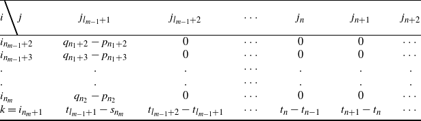
Suppose next that one of I or J is finite. Then, due to stochastic domination, the set I will have to be the one to be finite. Suppose
 $\max I = k$
. Then there will exist
$\max I = k$
. Then there will exist
 $m\in \mathbb{N}$
such that
$m\in \mathbb{N}$
such that
 $i_{n_m+1} = k$
. Then we define
$i_{n_m+1} = k$
. Then we define
 $\varepsilon_{i, j}$
in Table 2. To complete the proof, we need to show that
$\varepsilon_{i, j}$
in Table 2. To complete the proof, we need to show that
 \begin{equation} s_{n_m +1} = \lim_{n\to \infty}t_n. \end{equation}
This is because the sum of the kth row is
 $\lim_{n\to\infty}t_n - s_{n_m}$
. If (A.8) is true, then the kth row sum becomes
$\lim_{n\to\infty}t_n - s_{n_m}$
. If (A.8) is true, then the kth row sum becomes
 $q_k-p_k$
, which is as desired in (A.7). Now we show (A.8). Since I and J partition the natural numbers, we have
$q_k-p_k$
, which is as desired in (A.7). Now we show (A.8). Since I and J partition the natural numbers, we have
 $I\cup J = \mathbb{N}$
and thus
$I\cup J = \mathbb{N}$
and thus
 \begin{align*} &\sum_{i \in I \cup J}p_i = \sum_{j\in I \cup J}q_i = 1 , \quad \text{so that } \sum_{i\in I}p_i + \sum_{i\in J}p_i = \sum_{i\in I}q_i+ \sum_{j\in J}q_j.\end{align*}
In turn this implies that
 \begin{equation*} \sum_{i\in I}(p_i -q_i) = \sum_{j\in J}(q_j -p_j).\end{equation*}
Notice that, by definition,
 $\lim_{n\to \infty}t_n = \sum_{i\in I}(p_i -q_i)$
and
$\lim_{n\to \infty}t_n = \sum_{i\in I}(p_i -q_i)$
and
 $ s_{n_m +1} = \sum_{j\in J}(q_j -p_j)$
. This finishes the proof.
$ s_{n_m +1} = \sum_{j\in J}(q_j -p_j)$
. This finishes the proof.
Appendix B. Characterisation of stochastic ordering in
$\alpha$
-sequences

In this section, we prove Lemmas 3.5 and 3.6. By definition of stochastic domination,
 $\boldsymbol{r} \preccurlyeq_{\boldsymbol{p}} \boldsymbol{r}'\iff \boldsymbol{p}\boldsymbol{r} \preccurlyeq_{st} \boldsymbol{p}\boldsymbol{r}'.$
Thus Lemma 3.5 follows from Lemma A.2. Therefore we only prove Lemma 3.6.
$\boldsymbol{r} \preccurlyeq_{\boldsymbol{p}} \boldsymbol{r}'\iff \boldsymbol{p}\boldsymbol{r} \preccurlyeq_{st} \boldsymbol{p}\boldsymbol{r}'.$
Thus Lemma 3.5 follows from Lemma A.2. Therefore we only prove Lemma 3.6.
Proof of Lemma
3.6. We define our
 $\varepsilon$
-sequence
$\varepsilon$
-sequence
 $(\delta_i)_{i\geq 1}$
recursively. First we define
$(\delta_i)_{i\geq 1}$
recursively. First we define
 \begin{equation*} k_1 \;:\!=\; \begin{cases} \min \{n\in \mathbb{N}\colon r'_{\!\!n} < r_n \} & \text{if the minimum is attained}, \\[5pt] \infty & \text{otherwise}. \end{cases}\end{equation*}
We know that
 $k_1 >1$
, due to
$k_1 >1$
, due to
 $\boldsymbol{r}\preccurlyeq_{\boldsymbol{p}} \boldsymbol{r}'$
. Define
$\boldsymbol{r}\preccurlyeq_{\boldsymbol{p}} \boldsymbol{r}'$
. Define
 $\delta_i = r'_{\!\!i} - r_i$
for each
$\delta_i = r'_{\!\!i} - r_i$
for each
 $i<k_1$
. If
$i<k_1$
. If
 $k_1 = \infty$
, we define
$k_1 = \infty$
, we define
 $\delta_i=r'_{\!\!i} - r_i$
for all
$\delta_i=r'_{\!\!i} - r_i$
for all
 $i\in \mathbb{N}$
, so that, by definition of
$i\in \mathbb{N}$
, so that, by definition of
 $k_1$
,
$k_1$
,
 $\delta_i=r'_{\!\!i} - r_i\geq 0$
, and thus it satisfies the required condition. Suppose instead that
$\delta_i=r'_{\!\!i} - r_i\geq 0$
, and thus it satisfies the required condition. Suppose instead that
 $k_1<\infty$
. Then we define
$k_1<\infty$
. Then we define
 \begin{align*} l_1 = \min\Biggl\{n >k_1\colon \sum_{i=k_1}^{n}p_i(r'_{\!\!i} - r_i)>0\Biggr\}. \end{align*}
Since
 $\boldsymbol{r}\preccurlyeq_{\boldsymbol{p}} \boldsymbol{r}'$
and
$\boldsymbol{r}\preccurlyeq_{\boldsymbol{p}} \boldsymbol{r}'$
and
 $k_1<\infty$
, by definition we have
$k_1<\infty$
, by definition we have
 $\sum_{i=k_1}^{\infty}p_i(r'_{\!\!i} - r_i)>0$
. As a result, there exists m such that
$\sum_{i=k_1}^{\infty}p_i(r'_{\!\!i} - r_i)>0$
. As a result, there exists m such that
 $\sum_{i=k_1}^{m}p_i(r'_{\!\!i} - r_i)>0$
, which means that the set whose minimum we want to compute is non-empty. By the well ordering principle for natural numbers, we can conclude that the minimum is attained and thus
$\sum_{i=k_1}^{m}p_i(r'_{\!\!i} - r_i)>0$
, which means that the set whose minimum we want to compute is non-empty. By the well ordering principle for natural numbers, we can conclude that the minimum is attained and thus
 $l_1 < \infty$
. Having obtained
$l_1 < \infty$
. Having obtained
 $l_1 <\infty$
, we define
$l_1 <\infty$
, we define
 $\delta_i$
for all
$\delta_i$
for all
 $1 \leq i \leq l_1$
as
$1 \leq i \leq l_1$
as
 \begin{equation*} \delta_i \;:\!=\; \begin{cases} r'_{\!\!i} - r_i & \text{for }i<k_1, \\[5pt] 0 & \text{for }k_1\leq i< l_1, \\[5pt] \frac{1}{p_{l_1}}\sum_{i=k_1}^{l_1}(r'_{\!\!i}-r_i)p_i & \text{for }i = l_1. \end{cases}\end{equation*}
Next we define
 $k_2$
, similarly to
$k_2$
, similarly to
 $k_1$
, as
$k_1$
, as
 \begin{equation*} k_2 \;:\!=\; \begin{cases} \min \{n >l_1\colon r'_{\!\!n} < r_n\} & \text{if the minimum is attained}, \\[5pt] \infty & \text{otherwise}. \end{cases}\end{equation*}
If
 $k_2 = \infty$
, then we define
$k_2 = \infty$
, then we define
 $\delta_i=r'_{\!\!i} - r_i$
for all
$\delta_i=r'_{\!\!i} - r_i$
for all
 $i>l_1$
and it again satisfies the required condition. Suppose instead that
$i>l_1$
and it again satisfies the required condition. Suppose instead that
 $k_2<\infty$
. Then we define
$k_2<\infty$
. Then we define
 $l_2$
similarly to
$l_2$
similarly to
 $l_1$
as
$l_1$
as
 \begin{align*}l_2 = \min\Biggl\{n >k_2\colon \sum_{i=k_2}^{n}p_i(r'_{\!\!i} - r_i)>0\Biggr\}.\end{align*}
Since
 $\boldsymbol{r}\preccurlyeq_{\boldsymbol{p}} \boldsymbol{r}'$
, it can be shown that the above minimum is always attained and
$\boldsymbol{r}\preccurlyeq_{\boldsymbol{p}} \boldsymbol{r}'$
, it can be shown that the above minimum is always attained and
 $l_2<\infty$
. We define
$l_2<\infty$
. We define
 $\delta_i$
for all
$\delta_i$
for all
 $k_2 \leq i \leq l_2$
as
$k_2 \leq i \leq l_2$
as
 \begin{equation*} \delta_i \;:\!=\; \begin{cases} r'_{\!\!i} - r_i & \text{for }l_1\leq i<k_2, \\[5pt] 0 & \text{for }k_2\leq i< l_2, \\[5pt] \frac{1}{p_{l_1}}\sum_{i=k_1}^{l_1}(r'_{\!\!i}-r_i)p_i & \text{for }i = l_1. \end{cases}\end{equation*}
We keep on defining
 $k_i$
and
$k_i$
and
 $l_i$
similarly, unless
$l_i$
similarly, unless
 $k_i=\infty$
for some
$k_i=\infty$
for some
 $i\geq 1$
. In this way, we get the desired
$i\geq 1$
. In this way, we get the desired
 $\varepsilon$
-sequence iteratively.
$\varepsilon$
-sequence iteratively.
Funding information
This work is supported in part by the Netherlands Organisation for Scientific Research (NWO) through the Gravitation NETWORKS grant no. 024.002.003.
Competing interests
There were no competing interests to declare which arose during the preparation or publication process of this article.


 Open access