INTRODUCTION
In New Zealand, nitrous oxide (N2O) emissions from agricultural soils account for 13·6% of anthropogenic greenhouse gas emissions on a CO2-equivalent basis (Ministry for the Environment 2014). Of these, 56·3% are direct emissions from grazing animals’ excreta, 18·4% direct emissions from other sources of nitrogen (N) to soil (e.g. fertilizer, animal waste and crop residues) and 25·4% from indirect emissions. The present study focuses on direct emissions from urine patches, as the emissions from dung are comparatively small (van der Weerden et al. Reference van der Weerden, Luo, de Klein, Hoogendoorn, Littlejohn and Rys2011).
Nitrous oxide emissions have a high degree of spatial and temporal variability due to the complexity of the various interacting processes and variability of the driving factors (Mosier et al. Reference Mosier, Duxbury, Freney, Heinemeyer and Minami1996). A number of different factors, such as topography and soil properties, have been linked to spatial variability of N2O emissions (Parkin Reference Parkin1987; Pennock et al. Reference Pennock, van Kessel, Farrell and Sutherland1992; Velthof et al. Reference Velthof, Jarvis, Stein, Allen and Oenema1996, Reference Velthof, van Groenigen, Gebauer, Pietrzak, Jarvis, Pinto, Corré and Oenema2000; Ball et al. Reference Ball, Horgan, Clayton and Parker1997; Grant & Pattey Reference Grant and Pattey2003; Yanai et al. Reference Yanai, Sawamoto, Oe, Kusa, Yamakawa, Sakamoto, Naganawa, Inubushi, Hatano and Kosaki2003; Turner et al. Reference Turner, Chen, Galbally, Leuning, Edis, Li, Kelly and Phillips2008). In grazed pasture systems there is additional spatial variability due to the highly non-uniform nature of urine deposits (i.e. small areas of high N-concentration) (Bolan et al. Reference Bolan, Saggar, Luo, Bhandral and Singh2004). Previous studies have looked at the distribution of urine patches both experimentally (Moir et al. Reference Moir, Cameron, Di and Fertsak2011) and theoretically (Pleasants et al. Reference Pleasants, Shorten and Wake2007); however, these studies did not investigate N2O emissions. Giltrap et al. (Reference Giltrap, Berben, Palmada and Saggar2014) investigated the spatial variability of N2O emissions within a field and found differences in the emission response to applied urine at different locations.
Closed chambers are a relatively inexpensive method for measuring N2O emissions. In this method a number of chambers are inserted into the soil. The tops are then sealed to form closed chambers and the air within the headspaces sampled at regular intervals. The N2O flux is calculated from the change in N2O concentration over time. Sealing and sampling of the chambers can be automated or performed manually. Manual chambers in particular are relatively cheap to deploy, although the labour requirements increase as more chambers are used. International researchers have published guidelines on the use of chambers for N2O measurements (de Klein & Harvey Reference de Klein and Harvey2012). These guidelines do not specify a minimum number of chambers, but do state that chambers should cover the largest total area practicable while providing information at the smallest scale required.
Integrative, micrometeorological methods are an alternative to chamber measurements. These methods measure emissions over a wider spatial scale and are therefore less affected by spatial variability; however, there can be limitations due to weather conditions and topography. Also atmospheric N2O concentrations tend to be quite low, and may be close to the detection limit of many sensors.
Nitrous oxide emissions are frequently expressed in terms of an emission factor (EF). That is, the amount of N lost as N2O (in excess of any background emission rate) as a fraction of the amount of N input. However, EF values vary with soil properties, weather conditions and other factors. Almost 90% of the uncertainty in New Zealand's inventory value for N2O emissions from agricultural soil in 2002 (the relative error of the 95% confidence interval is –42% to +74%) was attributed to uncertainty in the value of EF (Ministry for the Environment 2014).
Studies for determining EF for animal urine in New Zealand used closed chambers to which known amounts of urine-N were applied (de Klein et al. Reference de Klein, Barton, Sherlock, Li and Littlejohn2003). This eliminated the variability due to uneven urine deposition, although there was still high variability in N2O emissions due to variability in soil properties (CV ranged from 22 to 55% for different sites). However, these types of experiments may not be completely representative of what occurs during an actual grazing event (e.g. effects such as compaction caused by animal treading and differences in urine concentration between animals are neglected). Some studies have been conducted to measure N2O emissions from actual grazed pastures (Saggar et al. Reference Saggar, Andrew, Tate, Hedley, Rodda and Townsend2004, Reference Saggar, Hedley, Giltrap and Lambie2007; Hoeft et al. Reference Hoeft, Steude, Wrage and Veldkamp2012; Luo et al. Reference Luo, Ledgard and Lindsey2013). These studies generally (although not always) used a larger number of chambers than the applied urine studies to account for the additional spatial variability of urine patch distribution. The question is how well can such a sample estimate the mean emissions from a field?
Many common statistical techniques assume that the data come from a normal distribution. This is clearly not the case for sampling a grazed pasture as there is both the probability of any given chamber landing on a urine patch combined with the variability of emissions from a urine patch. Neither is there an obvious transformation to normalize the data. However, according to the Central Limit Theorem (CLT), the arithmetic mean of a number (n) of independent random variables, each with a finite mean (μ) and variance (σ 2), will be approximately normally distributed with mean = μ and variance = σ 2/n as n → ∞ (Bain & Engelhardt Reference Bain and Engelhardt1992).
In the case of N2O emissions from grazed pastures, the distribution is highly skewed and it cannot be taken for granted that the CLT can be applied for practical sample sizes. To estimate the probability density function of the sampling distribution, computer simulations were used to generate a large number of samples from the underlying N2O emission distribution using a number of different sample sizes and assumptions about the properties of the underlying distribution. As the number of samples taken was large, the distribution of these samples should closely approximate the probability density function of the sampling distribution, and this distribution shall be referred to as the empirical sampling distribution (ESD). The properties of the ESDs were then examined to observe how they changed with different sample sizes and with changes to the underlying emission distribution. The arithmetic mean of each sample was initially used as the estimator of the mean of the underlying N2O emissions; some alternative estimators were then examined for comparison.
While the current research has been framed in terms of N2O measurements, the results may also be applicable to other situations where point measurements are made on a grazed field and the results are likely to be influenced by the presence or absence of a urine patch (e.g. nitrate leaching).
MATERIALS AND METHODS
Nitrous oxide emission model
For the simulations it was assumed that a number of chambers, n, were used to estimate the N2O emissions from a field following a grazing event. Each chamber had a probability, p, of landing on a urine patch, where p represents the proportion of the field covered by urine patches. This assumed that the total area of chambers was sufficiently small that p could be considered the same for all chambers. The possibility of overlapping urine patches or chambers having only part of their area on a urine patch was not considered.
As the present study was concerned with spatial rather than temporal variation, it was assumed that each chamber measured the total N2O emitted over time accurately and that the duration of the measurement campaign was long enough to capture all the additional N2O emissions due to the grazing event.
The following equations describe the N2O emissions measured in a single chamber:
where N2O–N is the total N emitted as N2O (kg N/ha), B is the background N2O emissions over the measurement period (kg N/ha), EF is the emission factor (which is specific to a given location and time period, in kg/kg) and U is the N concentration of the urine patch (kg N/ha).
This formulation assumed that EF and U were independent. Some studies have suggested that EF may increase with increasing N concentration (Kim et al. Reference Kim, Hernandez-Ramirez and Giltrap2013); however, de Klein et al. (Reference de Klein, Luo, Woodward, Styles, Wise, Lindsey and Cox2014) suggested that this dependency only occurs at low values, while Kelliher et al. (Reference Kelliher, Li and Nobel2014) found no dependency.
Simulations
Empirical sample distributions were generated by simulating 9999 random samples in R (R Foundation for Statistical Computing, http://www.r-project.org/) and were generated for different sample sizes, urine coverages and assumptions about the distribution of U and EF. Table 1 shows the parameters investigated and the range of values considered. The maximum value of n considered was 100 chambers, which is higher than generally used in practice but still potentially feasible. Increasing the maximum number of chambers will eventually result in the sample mean distribution approaching a normal distribution (by the CLT). However, in this case it would no longer be necessary to use the methods described in the present study.
Table 1. Parameters varied to investigate the effect on the sample mean distribution

The background emissions (B) were considered to have a constant value of 1 kg N/ha. While there is likely to be some variability in background emissions, this was not considered likely to be a major contributor to overall spatial variability.
Different underlying distributions were investigated for the urine concentration and EF. For urine, only the constant and normal distributions were considered, whereas for the EF, gradient and log-normal distributions were also examined.
In all cases the distributions were parameterized to have the same expected value (0·01 for EF and 1000 kg N/ha for urine concentration). The expected value of 0·01 for EF corresponds to the New Zealand specific value used in the national inventory for calculating N2O emissions from urine applied to soil (Ministry for the Environment 2014). However, measured EF values have a high degree of variability with a positive skew (de Klein et al. Reference de Klein, Barton, Sherlock, Li and Littlejohn2003). Therefore, for the normal distribution a standard deviation of 0·005 was selected to give the largest variability possible while keeping the EF positive within two standard deviations of the mean.
Few studies have measured the N loading in urine patches in terms of g N/ha (Selbie et al. Reference Selbie, Buckthought and Shepherd2015). Haynes & Williams (Reference Haynes and Williams1993) give a range of 8–15 g/l for urine N concentration, with urination volumes in the range 1·6–2·2 l and patch size 0·16–0·49 m2 for dairy cattle. The expected value of 1000 kg N/ha for urine patch N concentration in the present study is consistent with this and is a value often used in artificial urine patch experiments (e.g. Luo et al. Reference Luo, Lindsey and Ledgard2008). The distributions considered are described briefly below:
Constant distribution (Const) – assumes there is no variability in the underlying quantity. While this is unrealistic, it may be a reasonable approximation when the variability of the quantity is negligible compared with other sources of variability. For the urine concentration the constant value was 1000 kg N/ha, while for EF the constant value was 0·01.
Normal distribution (Norm) – commonly occurs in nature and many standard statistical methods assume a normal distribution. For the urine concentration the normal distribution was assumed to have mean = 1000 kg N/ha and standard deviation = 200 kg N/ha. For the EF distribution the mean was 0·01 and the standard deviation 0·005.
Gradient distribution (Grad) – this distribution simulates the case where the variation in EF is due to correlation with some property (e.g. soil moisture) that varies linearly across the field. Sampling a random location is therefore equivalent to drawing a sample from a uniform distribution. In these simulations, the minimum and maximum EF values were 0 and 0·02, respectively.
Log-normal distribution (LNorm) – the skew in the chamber samples may not be due solely to the patchy nature of the urine deposits, but may also reflect a skewness in the EF distribution. Studies looking at N2O emissions from known applications of urine N often find positively skewed results, suggesting this may be the case (e.g. van der Weerden et al. Reference van der Weerden, Luo, de Klein, Hoogendoorn, Littlejohn and Rys2011). Log-normal distributions frequently occur when several factors act in a multiplicative fashion. For example, N2O emission rates could be affected by soil moisture, temperature and availability of substrates. The expected value of the log-normal distribution is given by:
(3)where μ is the log-mean and σ is the log-standard deviation. For the log-normal EF simulations the log-mean was set to –5·105 and the log-standard deviation to 1. There are an infinite number of combinations of μ and σ that could be selected that satisfy E(X) = 0·01. The particular combination selected here resulted in a 95% confidence interval for EF of 0·00085–0·043. Note that due to rounding, the expected value of this distribution was 0·017% higher than the other distributions. $$E(X) = \exp \left( {\mu + \displaystyle{{\sigma ^2} \over 2}} \right)$$
Properties of the empirical distribution
Nitrous oxide emissions from grazed pastures are highly skewed and it cannot be taken for granted that the CLT can be applied for practical sample sizes. Empirical sample distributions were generated for a number of estimators (arithmetic mean, geometric mean and two methods of biased-corrected geometric mean of a sample) using different sample sizes and assumptions about the distributions of EF and U (e.g. constant, normal, gradient and log-normal). The influence of these changes on the properties of the sampling distribution was then investigated. The properties of the ESDs investigated were the mean, variance, relative bias (rBias), probability that given a sample was an underestimate of the true mean (pUnder) and skewness.
The true mean of the N2O emissions distribution is the expected value given by:
assuming that the EF is independent of the urine concentration. All the distributions examined were parameterized, so that E(EF) = 0·01 and E(U) = 1000 kg N/ha. Therefore, for an unbiased estimator the mean of the ESD should = 1 + 10p.
When the CLT applies, the arithmetic mean of a sample should have variance = σ 2/n. However, even when the CLT does not apply it is desirable for an estimator to have a low variance.
rBias was defined as:
where Mean(ESD) is the mean of the empirical sampling distribution and E(N2O) = 1 + 10p as shown above.
The pUnder is the proportion of samples that underestimate the true mean. In an unbiased, symmetrical distribution this should be 0·50. A pUnder that is much higher or lower than 0·50 indicates either asymmetry (skew) and/or bias. Note that in the absence of any variability in the urine concentration or EF, pUnder could be calculated using the binomial distribution.
Finally, skewness is defined as the third standardized moment of a distribution. Skewness should be 0 for a symmetric distribution (such as the Normal), positive or negative values indicate positive (right) or negative (left) skew, respectively.
It should be noted that a skewed distribution is not the same as a biased distribution. A biased distribution is one in which the expected value (average over a large number of samples) differs from the true mean. However, a skewed distribution could still produce the correct average over a large number of samples, even though there is a high probability of any individual sample being an under- (or over-) estimate.
Modelling the distribution properties
Having generated ESDs, the next step was to model how the properties of the sample distributions varied with sample size and with the properties of the underlying population distribution. The obvious explanatory variables were p and n, as well as the distributions assumed for the urine patch concentration (U dist) factors and the emission factor (EFdist). However, some non-linear terms also suggested themselves. The sampling distribution was related to the binomial distribution as the number of urine patches sampled would follow a binomial distribution. The variance of a binomial distribution is npq = np(1 − p) = np–np 2. Therefore np and p 2 were included. When the CLT applies the variance of the sample mean depends on 1/n, so 1/n was added to the list of explanatory variables. The terms n 2, 1/p, n/p and p/n were also considered.
For each variable the interactions with EFdist, U dist, and the EFdist : U dist interaction were considered. Thus the full model was:
where ‘*’ indicates that both main and interaction effects were considered.
The best model was initially selected using stepwise selection (with the Akaike Information Criterion [AIC] as the selection criterion), in both the forward and backward directions. However, in many cases the selected model still contained a large number of explanatory variables. These models were replaced with simplified models when it could be demonstrated that explanatory variables could be dropped while retaining satisfactory model performance (i.e. good explanatory power, lack of structure and constant variance in the residuals).
A standard linear model was applied for all properties except pUnder, for which a binomial generalized linear model was used.
Alternative estimators
Nitrous oxide emissions from grazed pastures are highly skewed and therefore sample sizes will probably need to be large before the CLT can be applied. However, it is sometimes possible to use data transformations to improve the normality of the data. In particular, log-transformations are commonly used to reduce positive skew.
The geometric mean (g) is the mathematical equivalent of back-transforming the mean of the log-transformed data and is given by:
 $$g = \left( {\mathop \prod \limits_{i = 1}^n {x_i}} \right)^{1/n} = \exp \left( {\displaystyle{{\mathop \sum \nolimits_{i = 1}^n {\log(x_i)} \over n}}} \right)$$
where x i is the ith observation and n is the number of observations.
Therefore, g could potentially be used as an alternative estimator to the arithmetic mean (a). Unfortunately g is a biased estimator, that is, its expected value is less than the true mean of the N2O distribution.
Assuming that the underlying N2O distribution was actually log-normal, then from Eqn (3) a reasonable correction factor might be exp(σ 2/2). Therefore the second alternative estimator investigated was:
where s 2 is the sample variance.
Neyman & Scott (Reference Neyman and Scott1960) gave bias-correction formulae for a number of variable transformations. However, for the log-transformation this requires solving a Bessel function of an imaginary argument. Given that the N2O distribution is not precisely log-normal a slightly simpler formula was used to calculate the correction factor: exp((1–1/n)s 2/2). When the Taylor expansion is applied to this correction factor it only differs from that of Neyman & Scott (Reference Neyman and Scott1960) for the third and higher terms. However, it does have the property that it approaches exp(s 2/2) as n → ∞. Therefore the final estimator considered was:
 $$g_{c2} = g \times {\exp}\left( {\left( {1 - \displaystyle{1 \over n}} \right)\displaystyle{{s^2} \over 2}} \right)$$
All simulations and analyses were performed using the R statistical software package version 3.0.2
RESULTS
Sample mean
Using the arithmetic mean (a) as the estimator for each simulated N2O sample and then fitting the sample mean (the mean of the 9999 randomly generated samples) to the proportion of urine coverage gave the following relationship:
 $$\eqalign{&{\rm Mean}(a) = 1 {\cdot} 01( \pm 0 {\cdot} 001) + 9 {\cdot} 9( \pm 0 {\cdot} 01)p, \cr & \quad R_{{\rm adj}}^2 = 0 {\cdot} 997}$$
where Mean(a) is the sample mean (using the arithmetic mean as the estimator for each sample).
This agrees fairly well with the true mean as expressed in Eqn (4), indicating that the arithmetic mean is largely unbiased irrespective of the number of chambers used or the underlying distributions of the urine concentration or EF.
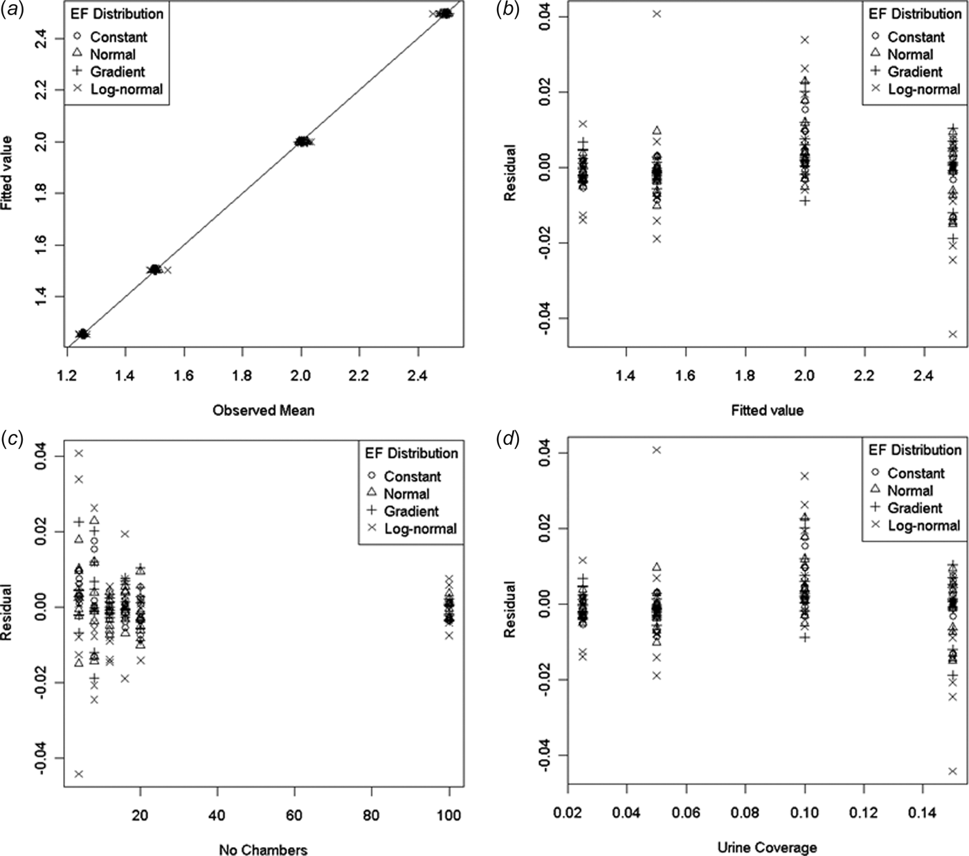
Figure 1 shows the modelled means (values calculated from Eqn (10)) plotted against the observed values (simulated sample means) as well as the residuals plotted against fitted values, n and p. There was an obvious decrease in the variability of the residuals as n increased. It was also apparent that the largest residuals correspond to the log-normal EF distribution. However, the largest relative residual was still quite small at only 3% of the fitted value.

Fig. 1. Plots comparing values fitted using model (10) with the observed mean of the ESD for a (arithmetic mean of a sample): (a) Fitted value v. observed mean, (b) residuals v. fitted values, (c) residuals v. number of chambers (n), (d) residuals v. urine coverage (p).
Variance
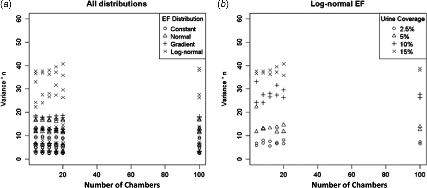
Figure 2 shows a plot of Var(a) × n v. n. When the CLT applies Var(a) → σ 2/n, in which case Var(a) × n should be constant with respect to n. From Fig. 2(a) this appears to be the case for all but the log-normal EF distribution. The log-normal EF distribution shows variability in Var(a) × n for different n (but not in any easily to discernible pattern, Fig. 2(b)).

Fig. 2. The variance of the ESD for a × n (arithmetic mean times the number of chambers) plotted against the number of chambers (should be constant if CLT applies). (a) All EF distributions and (b) log-normal EF only.
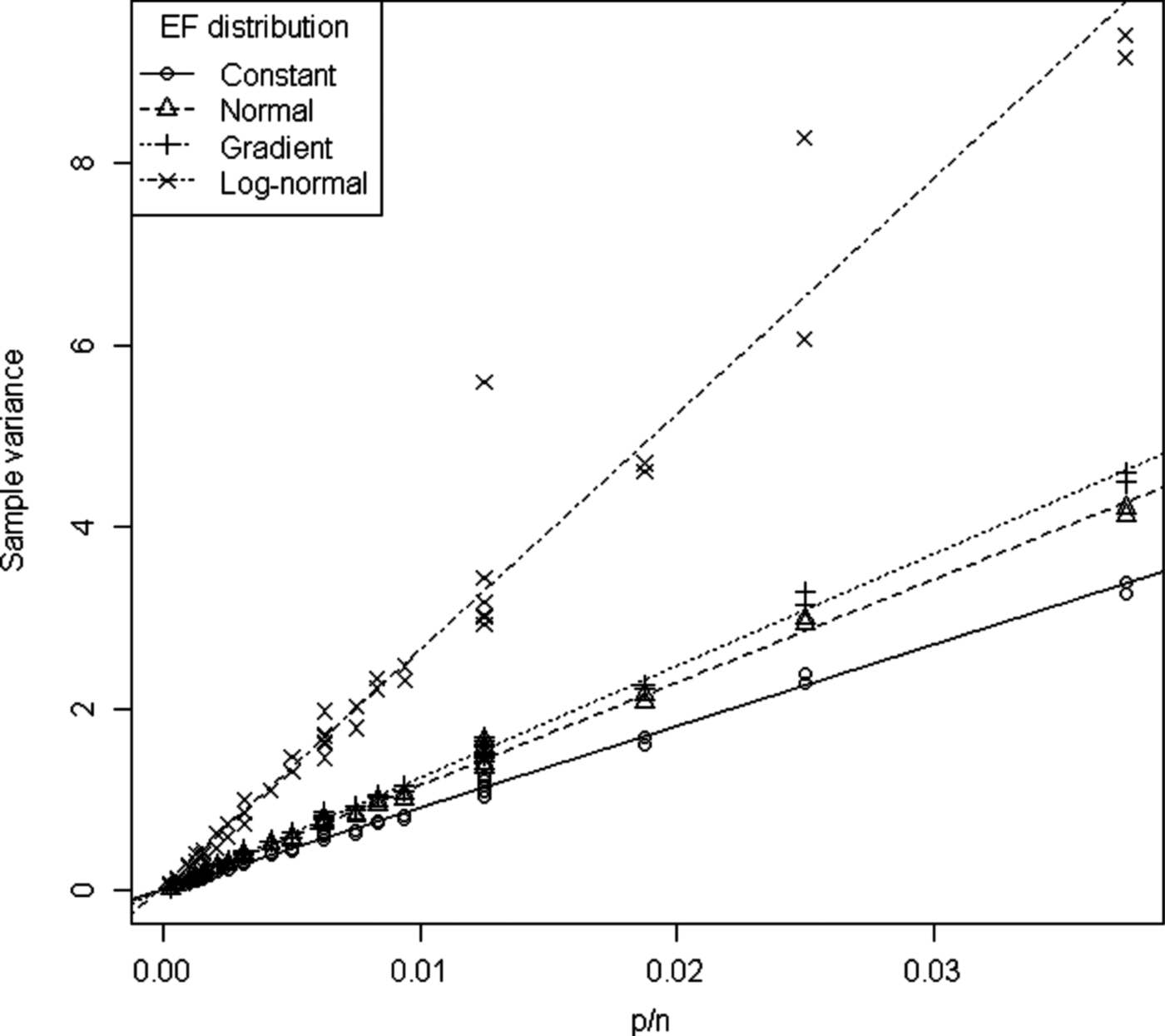
The variance could be quite well explained by a model involving p/n, EF DIST and their interaction (Eqn (11)).
 $$\eqalign{&{\rm Var}(a) \sim p/n + {\rm EF}_{{\rm DIST}} + {\rm EF}_{{\rm DIST}} :p/n, \cr & \quad R_{{\rm adj}}^2 = 0 {\cdot} 9753}$$
According to Eqn (11) the variance depends on the EF distribution and increases with p/n. The model is a reasonable approximation for the constant, normal and gradient EF distributions, but there are some large residuals for the log-normal EF distribution (Fig. 3). The variance was always highest for the log-normal EF distribution. For low p/n values the constant, normal, gradient EF distributions have similar variances. As p/n increases the variances of the different EF distributions diverge.

Fig. 3. Var(a) v. p/n. Straight lines indicate model (11) estimates.
Equation (11) is useful for determining the level of precision with which the mean can be determined. For example, suppose P = 0·05, n = 20. The variance of the sample mean would be 0·24 for a constant EF, corresponding to a standard deviation of 0·49 kg N/ha or 33% of the true mean. If the EF was normally distributed instead, then the standard deviation would be 38% of the true mean.
Relationship between mean and variance
The mean and variance appear to behave in a manner consistent with the CLT (with the exception of the variance when using the log-normal EF distribution). However, another requirement for a normal distribution is that the variance and mean should be independent. This is also an important assumption of linear regression.
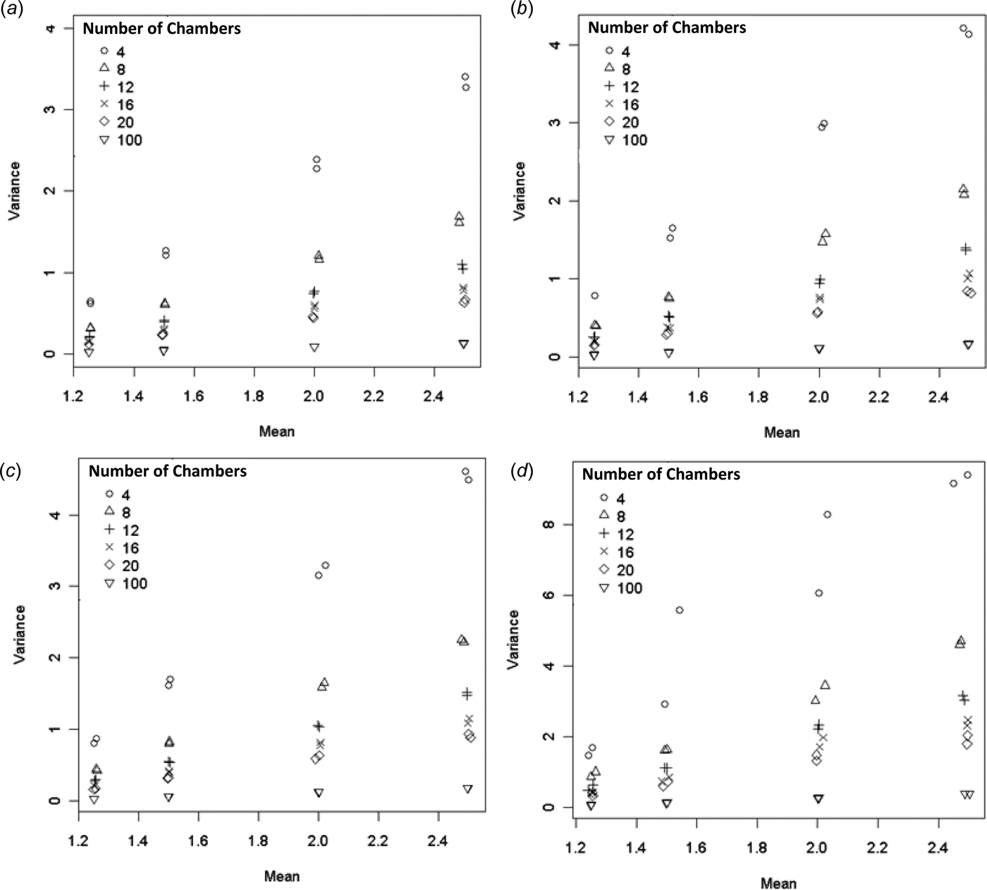
From inspection of models (10) and (11) it can be seen that both the mean and variance depend on p. Therefore, it seems likely that the mean and variance will be correlated. This is confirmed in Fig. 4. However, the slope of the relationship between variance and mean decreases as n increases, and for n = 100 the variance is almost constant with respect to the mean.

Fig. 4. Var(a) v. mean(a) for (a) constant, (b) normal, (c) gradient and (d) log-normal EF distributions.
The significance of the slopes of the relationships between variance and mean were determined by fitting a linear regression model of the variance of the ESD. The predictors were the mean of the ESD, a 24-level factor (EF_n) with each level corresponding to a combination of EF distribution and number of chambers, and their interactions (Eqn (12)). The following relationship was fitted:
With the exception of the levels corresponding to n = 100, all the coefficients for the EF_n interaction with the ESD mean were significantly different from 0 (at a 0·01 confidence level). None of the EF_n:Mean interaction coefficients were significant for n = 100 (at a 0·1 confidence level). Therefore the variance of the sample mean depends on the sample mean for the chamber numbers used in practice. However, at 100 chambers the variance was independent of the mean. This relationship held across all EF distributions.
As a consequence of this dependence of the variance on the mean (for n < 100) ordinary linear regression methods (including ANOVA) should not be performed on samples of this type. However, this can be corrected using a weighted regression provided the relationship between the mean and the variance is known. If the variance can be written as:
then the weighted regression can be performed using 1/f(μ i) as weights. There are several options for f(μ i). Using model (12) gives f(μ i) = ![]() $\bar x$. This assumes the same n and EF for all samples and will be slightly inaccurate due to neglecting the constant term. If the EF distribution is known, then the more precise form of f(μ i) =
$\bar x$. This assumes the same n and EF for all samples and will be slightly inaccurate due to neglecting the constant term. If the EF distribution is known, then the more precise form of f(μ i) = ![]() $a + b\bar x$ can be used. Alternatively, model (11) gives f(μi) = p/n. The constant terms in model (11) are not statistically significant, so can justifiably be neglected. If the urine coverage can be assumed to be constant, then it can be incorporated into σ 2 leaving f(μi) = 1/n.
$a + b\bar x$ can be used. Alternatively, model (11) gives f(μi) = p/n. The constant terms in model (11) are not statistically significant, so can justifiably be neglected. If the urine coverage can be assumed to be constant, then it can be incorporated into σ 2 leaving f(μi) = 1/n.
Relative bias
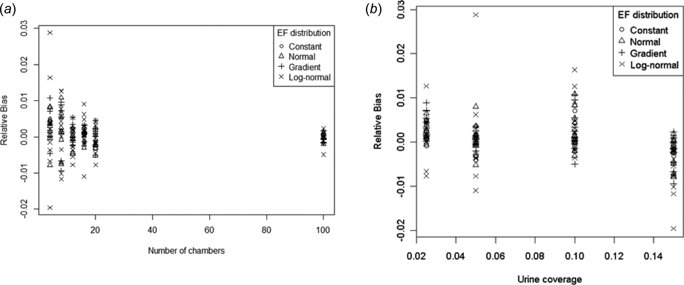
Earlier it was found that the mean of the ESDs were very close to the theoretical population means (Eqn (10)). Therefore bias should be small. Figure 5 shows the bias (relative to the mean) plotted against p and n.

Fig. 5. Relative bias v. (a) number of chambers and (b) urine coverage.
It is difficult to discern any patterns from these plots, although the variability in the rBias reduces with increasing n. However, the most extreme rBias values are only –2% and +3%, both of which occur for log-normal distributions.
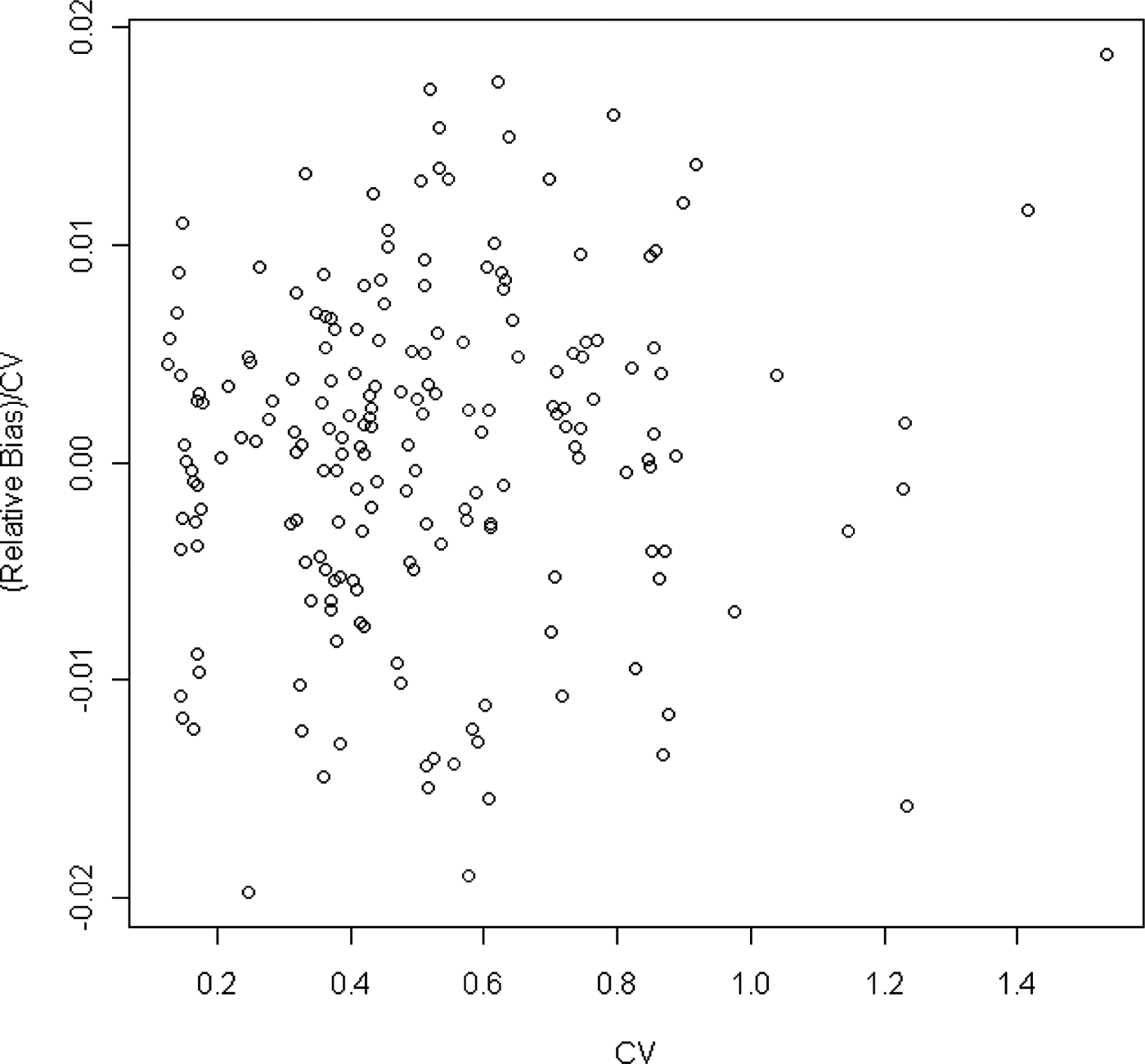
Bias becomes important when it is high relative to the variability. One measure of the relative importance of the bias would be to take the ratio of the bias to the standard deviation. This is equivalent to the ratio of the rBias to the CV. Figure 6 shows that the magnitude of the rBias is at most 2% of the CV. That is, the absolute bias is at most 2% of the standard deviation of the sample mean and therefore not a major concern.

Fig. 6. Ratio of relative bias to CV plotted against CV.
Probability that a given sample was an underestimate of the true mean (pUnder)
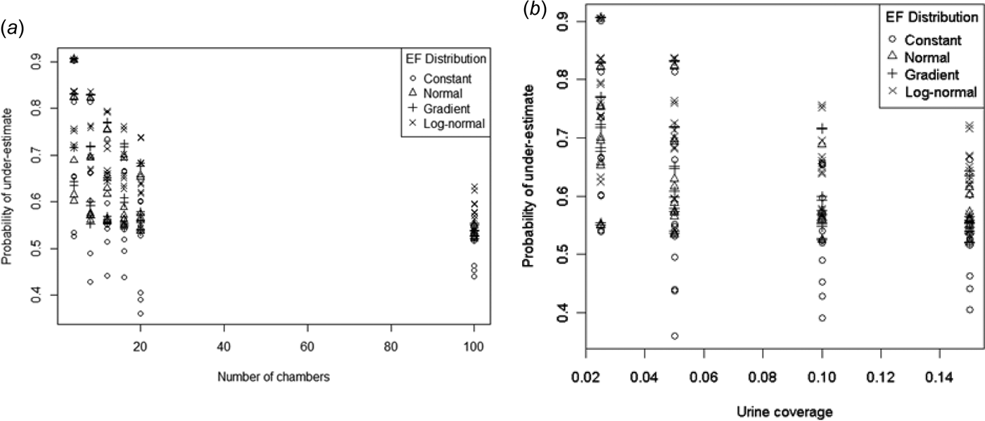
With the exception of some constant EF distribution points, pUnder was > 0·5 (Fig. 7). Both pUnder and the spread of pUnder decreased with increasing number of chambers and urine coverage. Even with 100 chambers the probability of underestimating the mean can be much larger than 0·5. Given that no evidence of bias was found in the sample mean distribution, these high pUnder values indicate a right-skewed distribution.

Fig. 7. Probability of a sample mean being less than the true mean by (a) number of chambers and (b) urine coverage.
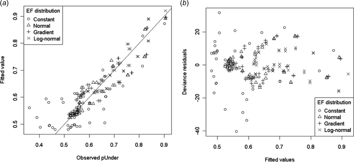
pUnder is a probability and therefore bounded by 0 and 1. Therefore a binomial generalized linear model with a logitFootnote † link function (Eqn (14)) was used for modelling:

Model (14) produced a reasonable fit for all but the constant EF distribution (Fig. 8). As an example, a sample from a normal EF distribution with n = 20 and P = 0·05 would have log-odds of 0·42 of being an underestimate. This corresponds to a pUnder of 60%, indicating a slight right-skew in the sample mean distribution.

Fig. 8. (a) Modelled v. observed pUnder and (b) deviance residuals v. fitted values for model (14).
Skewness
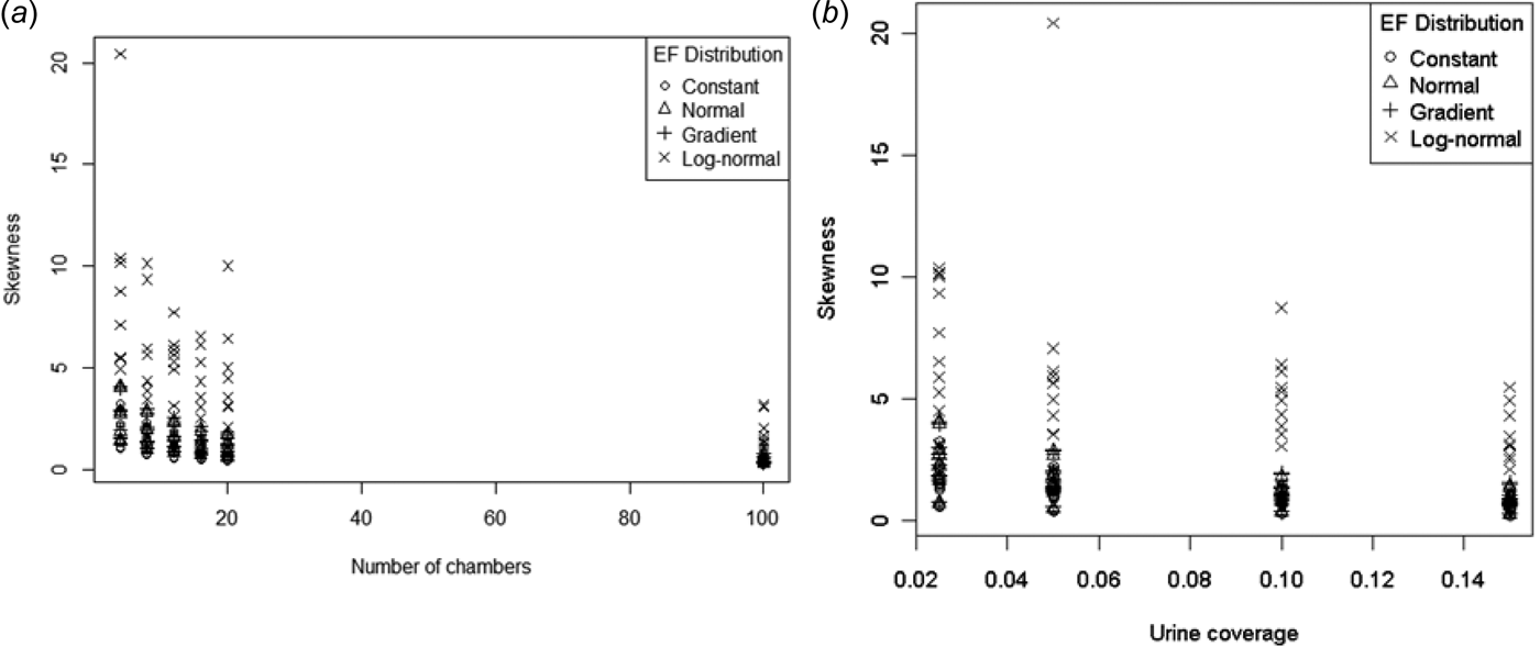
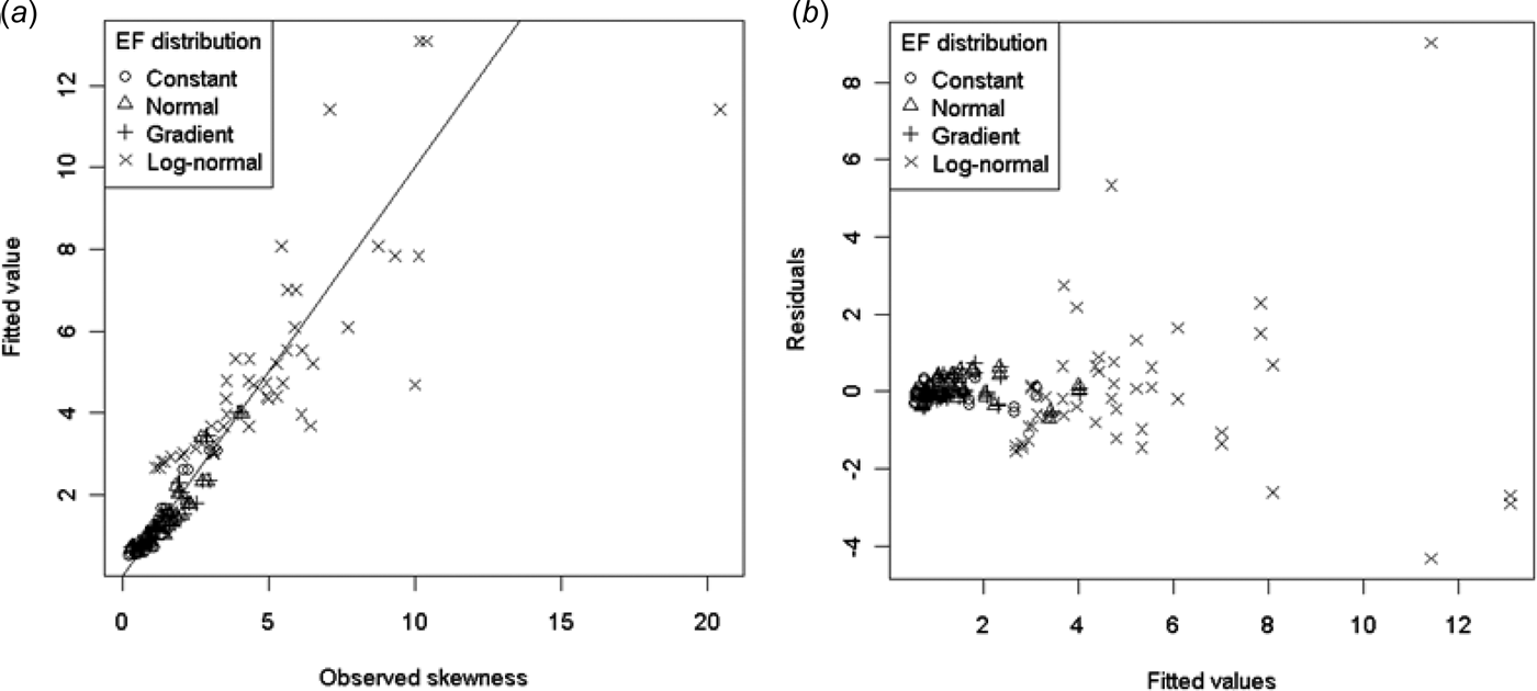
Skewness is the third standardized moment and relates to the lack of symmetry in a distribution. Skewness should be 0 for a symmetric distribution (such as the normal). Figure 9 shows the observed skewness of the sample mean distribution plotted as a function of number of chambers and urine coverage. Unsurprisingly, skewness was largest for the right-skewed log-normal EF distribution. Skewness reduced with increasing number of chambers, but remained positive over the range of conditions tested. There did not seem to be an obvious pattern to skewness with increasing urine coverage. Model (15) below produced a reasonable fit to the data, except for the log-normal EF distribution (Fig. 10.):
 $$\eqalign{&{\rm Skewness}\,(a) \sim {\rm EF}_{{\rm dist}} + 1/n + p/n + {\rm EF}_{{\rm dist}} \cr & \quad \quad \quad :1/n + {\rm EF}_{{\rm dist}} :p/n, \cr & \quad R_{{\rm adj}}^2 = 0 {\cdot} 8075}$$
Fig. 9. ESD Skewness as a function of (a) number of chambers and (b) urine coverage.

Fig. 10. (a) Modelled v. observed skewness and (b) residuals v. fitted values for model (15).

In model (15) only the log-normal EF distribution terms were significantly different from the constant EF distribution. The variability of the residuals increased with increasing skewness (Fig. 10.(b)). As the highest skewness occurred in the log-normal EF distribution, this distribution resulted in some large residuals and indicated that a better model of skewness may be required for log-normal EF distributions.
For the other EF distributions, model (15) indicates that for low values of p there will always be positive skewness regardless of the size of n. This threshold for p ranges from 0·168 to 0·178 depending on the EF distribution. This is higher than the maximum urine coverage considered in the present study (0·15), indicating that skewness cannot be eliminated for the range of urine coverages likely to be found in the field. Increasing p decreased skewness, but as n increases the skewness approaches a non-zero value (which depends on the EF distribution). By this model it is not possible to eliminate the skewness by increasing the sample size. While the CLT means the skewness should approach 0 for sufficiently high n, this must happen at n values well beyond those simulated in the present study, for which model (15) is valid.
Model (15) can be applied to constant, normal or uniform EF distributions, but is not recommended for log-normal EF-distributions. It also requires knowledge of the number of chambers and urine coverage. For 20 chambers and P = 0·05, a 20% increase in p resulted in a ~4% reduction in skewness, while a 20% increase in n resulted in a 7–8% decrease in skewness for the constant, normal and gradient EF distributions.
ALTERNATIVE ESTIMATORS
Mean
Fitting a linear regression of the alternative estimators on p gave the following relationships:
 $$\eqalign{{\rm Mean}\,(g) &= 0 {\cdot} 984\,( \pm \,0 {\cdot} 0051) + 3 {\cdot} 02\,( \pm \,0 {\cdot} 054)p,\cr R_{{\rm adj}}^2 &= 0 {\cdot} 94} $$
 $$\eqalign{&{\rm Mean}\,(g_{c1} ) = 0 {\cdot} 94\,( \pm \,0 {\cdot} 031) + 9 {\cdot} 0\,( \pm \,0 {\cdot} 33)p,\cr &\quad R_{{\rm adj}}^2 = 0 {\cdot} 80}$$
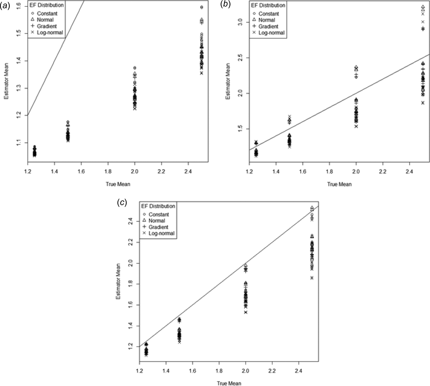
The geometric mean seriously underestimates the N2O emissions, with the coefficient of p being less than one-third of what it should be. The first corrected geometric mean g c1 gets much closer to the true mean, but not quite as close as the arithmetic mean (Eqn (10)). The second corrected mean (g c2) also performs much better than the uncorrected g but still underestimates by more than g c1.
For all estimators the variability increased as the mean increased (Fig. 11.).

Fig. 11. Mean of the ESD plotted against the true mean for (a) geometric mean (g), (b) first corrected geometric mean g c1 and (c) second corrected geometric mean g c2. The 1–1 line is also indicated.
rBias
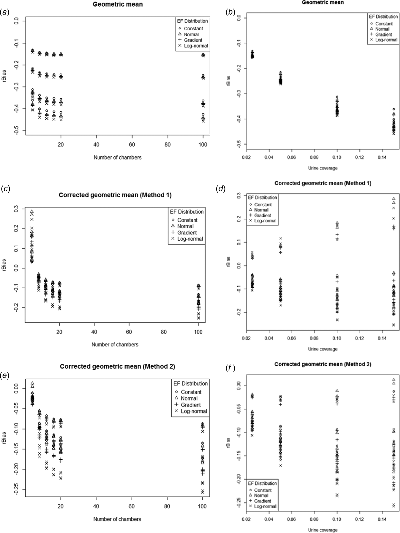
Figure 12 shows rBias plotted against n and p for each of the three alternative estimators. The three estimators generally had negative bias, although g c1 actually had a strong positive bias for n = 4. The bias was strongest in the uncorrected geometric mean. The rBias for g c2 was always more negative than g c1 but the difference approached 0 as the number of chambers increased. However, in terms of the magnitude of the bias, g c2 was actually less biased than g c1 for n = 4, but more biased at higher n. rBias decreased slightly (became more negative) then stabilized with increasing n for all three estimators. g showed a strong negative trend (i.e. became more biased) with increasing p, whereas the two bias-corrected geometric means had increasing variability in rBias as urine coverage increased. The range of rBias was from –13 to –46% for g, –26 to +29% for g c1, and –26 to +1·3% for g c2. These are large compared with the relative biases of a.

Fig. 12. rBias plotted against number of chambers (a, c, e) and urine coverage (b, d, f) for geometric mean (a, b), first corrected geometric mean (c, d), second corrected geometric mean (e, f).
Variance
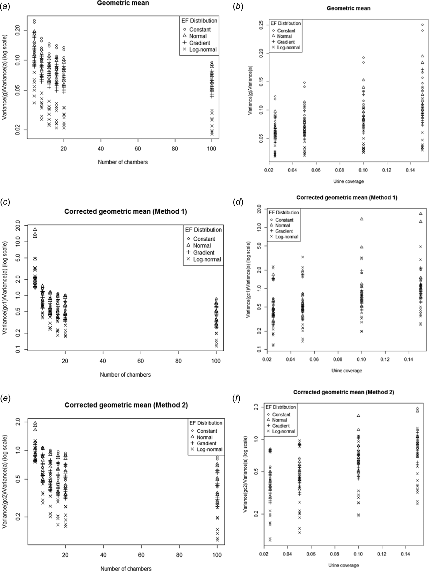
The uncorrected geometric mean consistently had a lower variance than the arithmetic mean (variance ratio < 1, Fig. 13.). Given that low variance is a desirable property, the relative advantage (from a variance perspective) of g relative to a increases as n increases but decreases with increasing p. In Fig. 2, it was seen that for most cases Var(a) was inversely proportional n. Therefore the variance of g must decrease even more rapidly with n.

Fig. 13. Ratio of the variance of g, g c1 and g c2 to the variance of a plotted against the number of chambers (a, c, e) and urine coverage (b, d, f). Note log scale on the y-axis for the corrected geometric means.
The bias corrections for the geometric mean use the sample standard deviation of the log-transformed data to estimate the population log-standard deviation. Unfortunately, this increases the variance relative to the uncorrected geometric mean. For low sample sizes the corrected geometric means can sometimes have larger variances than the arithmetic mean. Both the corrected geometric means show similar trends in variance relative to Var(a) with increasing n and p. The second bias correction method always produced a lower variance than the first, although the difference decreased as the number of chambers increased.
For all three alternative estimators the relative improvement in variance over the arithmetic mean was greatest when the EF distribution was log-normal.
Skewness
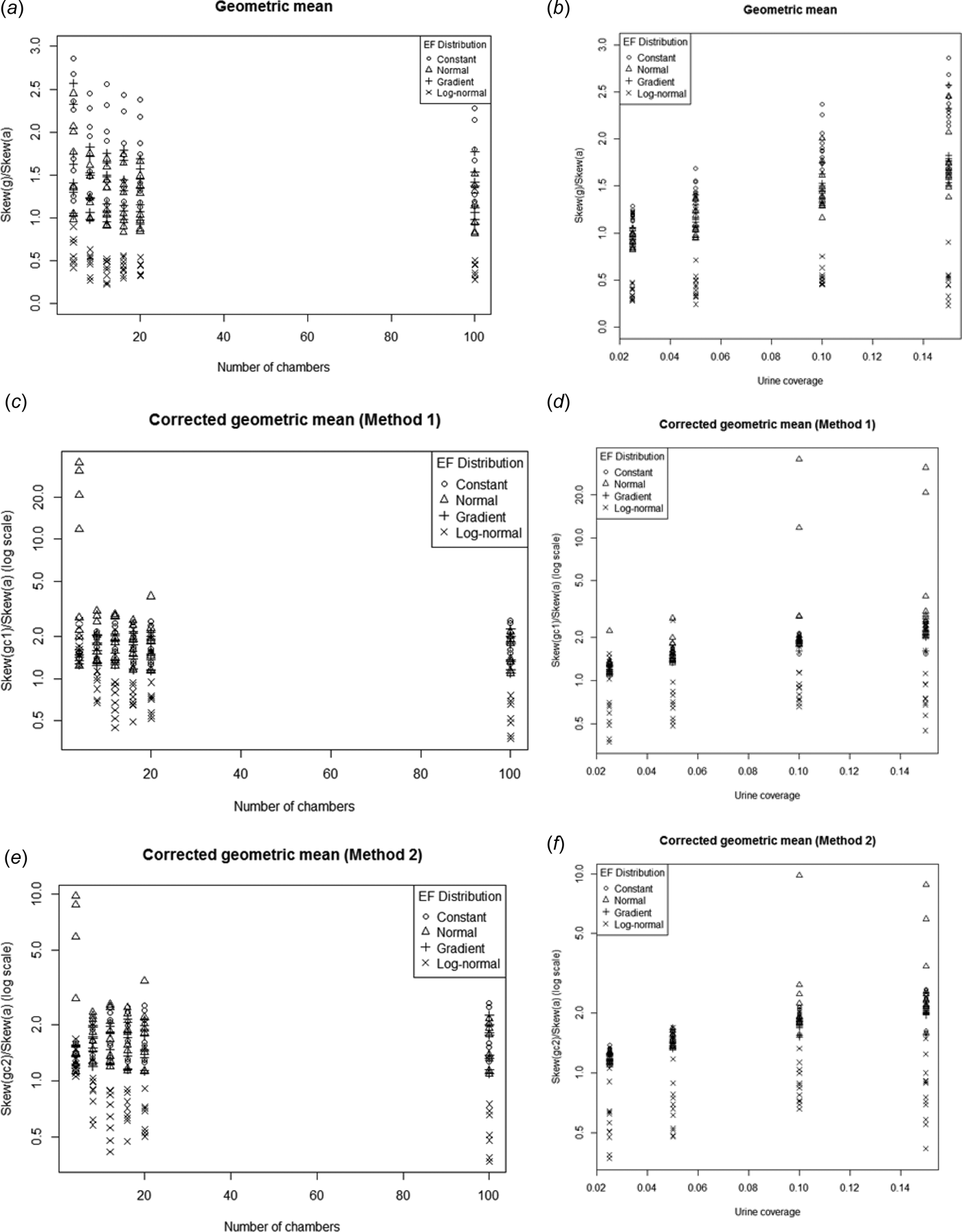
None of the estimators consistently reduced (or increased) the skew relative to the arithmetic mean (Fig. 14.). In general, for log-normal EF the geometric mean (and the corrected versions) tended to have lower skew than the arithmetic mean. For the other EF distributions the skew tended to be higher than the arithmetic mean.

Fig. 14. Ratio of the skewness of g, g c1 and g c2 to the skewness of a plotted against number of chambers (a, c, e) and urine coverage (b, d, f). Note log scale on the y-axis for the corrected geometric means.
DISCUSSION
The arithmetic mean of chamber measurements was an unbiased estimator of the N2O emissions from a grazed pasture. However, the CLT did not apply over the range of conditions examined (even with 100 chambers) and the sample mean distribution was right-skewed. The variance was relatively high (with standard deviation ranging from 12 to 135% of the actual mean) but did appear to be proportional to 1/n except when the EF distribution was log-normal. For n < 100 the variance was proportional to the mean, therefore attempts to use regression modelling on chamber data should include weights to account for the non-constant variance. The lack of normality means that statistical tests that assume normality of the sample mean (e.g. t-test and F-test) should not be used for this type of data. With knowledge of the urine coverage and EF distribution, equivalent tests could be created by generating empirical sampling distributions as we have done here. However these tests would probably have lower power due to the high probability of not sampling any urine patches.
Formulae were derived that gave reasonable estimates for variance, pUnder and skewness of the sample distribution of the arithmetic mean. These formulae required knowledge of the number of chambers, the urine coverage and the EF distribution. Whether the urine concentration was constant or normally distributed had little impact on the sample mean distribution. An experimenter will know the number of chambers being used, but will not know the urine coverage or the EF distribution. However, there are methods for estimating the urine coverage if the number of animals grazed and the duration of the grazing event are known (e.g. Pleasants et al. Reference Pleasants, Shorten and Wake2007) and there have recently been some studies looking at measuring urine patch concentration experimentally (Moir et al. Reference Moir, Cameron, Di and Fertsak2011). The EF distribution is trickier. In particular, the formulae for variance and skewness are poor predictors when the EF distribution is log-normal. Therefore determining the nature of the EF distribution should be a priority.
Some alternative estimators were also examined. Log-transformations are commonly used to make right-skewed data more symmetrical. The geometric mean is the mathematical equivalent of back-transforming the mean of the log-transformed data. Unfortunately, the geometric mean was a biased estimator that consistently underestimated the true mean, and although the geometric mean did have a lower variance than the arithmetic mean, it did not necessarily have less skew. Still, the lower variance of the geometric mean could make it a useful estimator for situations where the aim is to compare N2O emissions from different treatments, rather than to estimate the actual emissions.
Two methods for bias-correcting the geometric mean were also investigated. These methods both used the sample standard deviation of the log-transformed data to calculate the bias correction. While these methods did reduce the bias they also had the unfortunate side effect of increasing the variance. None of the alternative estimators universally outperformed the arithmetic mean. However, in some circumstances (e.g. when the EF distribution is log-normal) a bias-corrected geometric mean might make a better estimator, but this would need to be determined on a case-by-case basis.
A number of simplifying assumptions were made for the current simulations, which included that the urine patches did not overlap and that the EF was independent of the urine concentration. The first assumption is more likely to be satisfied when stocking rates are low and grazing durations short. According to the method of Pleasants et al. (Reference Pleasants, Shorten and Wake2007) with the mean patch area (0·37 m2) and urination rate (0·53 events/cow/hour) measured by Moir et al. (Reference Moir, Cameron, Di and Fertsak2011), one day grazing at a stocking density of 180 cows/ha would result in 0·081 of the area being covered by urine patches, but 0·96 of the urine patch area would be single urine patches. So overlapping urine patches would account for only 0·003 of the total area. However, this assumes that the distribution of urine patches is completely random. In reality, animal behaviour is likely to result in non-random urine patch distribution. For example, urine patches are likely to be more frequent in areas where animals congregate (e.g. near water troughs or shelter), but there could also be a tendency to avoid grazing near existing urine patches. The measurements of Moir et al. (Reference Moir, Cameron, Di and Fertsak2011) found urine patch coverage in a season ranged from 0·035 to 0·076 with cow-days/ha/season ranging from 120 to 450. This lower coverage indicates a higher rate of overlap than estimated using the Pleasants method.
The second assumption requires that the relationship between N2O emissions and urine N concentration be linear. Kim et al. (Reference Kim, Hernandez-Ramirez and Giltrap2013) hypothesized that the relationship between N2O emissions and applied N could have linear and non-linear phases depending on the limiting process. Kelliher et al. (Reference Kelliher, Li and Nobel2014) found a strong linear relationship between N2O emissions and applied N, but no significant quadratic term for urea applied at rates of 25 to 1500 kg N/ha. However, in a field study, de Klein et al. (Reference de Klein, Luo, Woodward, Styles, Wise, Lindsey and Cox2014) found an increasing trend of EF with urine N concentration in a free-draining soil, but not on a poorly draining soil. In addition to a direct relationship between urine concentration and EF, there could also be an indirect effect if the spatial variability of EF was driven by some factor (such as soil moisture or slope) that also affects the amount of time the animals spend in a given part of the field.
The present study also did not consider the effect of using different means and standard deviations for the EF and U concentrations. This is an area that could be further investigated if more data regarding these distributions were available. However, completely random sampling on a grazed pasture is always going to be problematic due to the large difference between the emissions from urine and non-urine patches and the lack of knowledge of the number of urine patches included in a given sample. If non-destructive methods for determining the urine patch locations shortly after a grazing event can be developed then a stratified sampling scheme could be used to give more robust estimates of emissions. Alternatively, if the presence or absence of a urine patch in each chamber could be conclusively determined after the fact (e.g. from soil properties or grass growth), then the relative contribution from the urine and non-urine containing chambers could be scaled according to the overall urine coverage. The method of applying a known amount of urine-N to each chamber avoids the errors introduced by not knowing the location of the urine patches, but requires the total amount of urine-N excreted during grazing to be estimated, which may miss effects caused by animal behaviour (e.g. treading).
CONCLUSIONS
In the present study formulae were derived that can be used to calculate the mean, bias, variance and skewness of the sample distribution when measuring N2O emissions using chambers on a grazed pasture. These formulae require knowledge of the fractional area covered by urine patches, number of chambers, and the nature of the EF distribution.
The arithmetic mean was an unbiased estimator, and over a large number of trials the mean of all the samples will approach the true value. Unfortunately, the sample mean distribution had a high variance and skew. This meant for any particular trial the sample mean could be a long way from the true value and there was a >50% chance that any given sample would be an underestimate. The CLT did not apply for realistic numbers of chambers, therefore many common statistical techniques requiring normal data (e.g. t-tests and F-tests) should not be applied to data of this type. The behaviour of the sample mean distribution did not depend on whether the urine concentration was constant or normally distributed, but did depend on the distribution of the EF.
The geometric mean had lower variance, but high bias compared with the arithmetic mean. Two bias corrections for the geometric mean were tried. These methods did reduce the bias of the geometric mean, but as the corrections used estimates of the standard deviation, the variances were high. The corrected geometric means were not a universal improvement on the arithmetic mean, although in some circumstances they had lower variances and skewness (e.g. when the EF was log-normally distributed and n > 4). However, all these alternative estimators still suffered from non-normality.
The best way to improve the estimation of N2O emissions from a grazed pasture would be to sample separately from known urine and non-urine patch areas. This, however, requires the development of a non-disruptive method for identifying urine patches shortly after a grazing event. In the absence of such a method there will always be some inherent problems (e.g. skewness) in the sample mean distribution. The distribution of the EF was also an important factor in the properties of the sample mean distribution. Knowledge of how the EF varies spatially is therefore useful for determining the properties of the sample mean distribution.
This research was supported by Core funding for Crown research institutes from the Ministry of Business, Innovation and Employment's Science and Innovation Group. The authors thank Andrew McMillan for his helpful comments on the draft paper and Anne Austin for internal editing.

