


1 Introduction
Beams of MeV-energy fast electrons can be created via irradiation of high-intensity
 $\left(I{\lambda}^2>{10}^{18}\;{\mathrm{W}\ \mathrm{cm}}^{-2}\ {\mu \mathrm{m}}^2\right)$
, femtosecond laser pulses with solid targets. These fast electrons propagate through the target and are the driver of much of the downstream physics during the interaction. As the fast electron beam propagates through the target it induces bremsstrahlung emission that can be used as a high-energy X-ray source for radiography[
Reference Brenner, Mirfayzi, Rusby, Armstrong, Alejo, Wilson, Clarke, Ahmed, Butler, Haddock, Higginson, McClymont, Murphy, Notley, Oliver, Allott, Hernandez-Gomez, Kar, McKenna and Neely1]. The fast electrons additionally cause fluorescence of k
$\left(I{\lambda}^2>{10}^{18}\;{\mathrm{W}\ \mathrm{cm}}^{-2}\ {\mu \mathrm{m}}^2\right)$
, femtosecond laser pulses with solid targets. These fast electrons propagate through the target and are the driver of much of the downstream physics during the interaction. As the fast electron beam propagates through the target it induces bremsstrahlung emission that can be used as a high-energy X-ray source for radiography[
Reference Brenner, Mirfayzi, Rusby, Armstrong, Alejo, Wilson, Clarke, Ahmed, Butler, Haddock, Higginson, McClymont, Murphy, Notley, Oliver, Allott, Hernandez-Gomez, Kar, McKenna and Neely1]. The fast electrons additionally cause fluorescence of k
 $\unicode{x3b1}$
X-rays in the material, enabling the characterization of warm dense matter produced in the interaction[
Reference Gizzi, Giulietti, Giulietti, Köster, Labate, Levato, Zamponi, Lübcke, Kämpfer, Uschmann, Förster, Antonicci and Batani2,
Reference Köster, Akli, Batani, Baton, Evans, Giulietti, Giulietti, Gizzi, Green, Koenig, Labate, Morace, Norreys, Perez, Waugh, Woolsey and Lancaster3]. The highest energy electrons can escape the target at the rear surface[
Reference Rusby, Armstrong, Scott, King, McKenna and Neely4], driving an electrostatic sheath field that can additionally accelerate protons up to MeV energies[
Reference Snavely, Key, Hatchett, Cowan, Roth, Phillips, Stoyer, Henry, Sangster, Singh, Wilks, Mackinnon, Offenberger, Pennington, Yasuike, Langdon, Lasinski, Johnson, Perry and Campbell5–
Reference Sentoku, Cowan, Kemp and Ruhl7]. These ion beams could find use in medical applications[
Reference Malka, Fritzler, Lefebvre, d’Humières, Ferrand, Grillon, Albaret, Meyroneinc, Chambaret, Antonetti and Hulin8] and as a source of protons for diagnosing warm, dense matter[
Reference Malko, Cayzac, Ospina-Bohórquez, Bhutwala, Bailly-Grandvaux, McGuffey, Fedosejevs, Vaisseau, Tauschwitz, Apiñaniz, De Luis Blanco, Gatti, Huault, Hernandez, Hu, White, Collins, Nichols, Neumayer, Faussurier, Vorberger, Prestopino, Verona, Santos, Batani, Beg, Roso and Volpe9]. Moreover, the fast electron beam itself has been proposed as an igniter in the fast ignition (FI) variant of inertial confinement fusion[
Reference Tabak, Hammer, Glinsky, Kruer, Wilks, Woodworth, Campbell, Perry and Mason10].
$\unicode{x3b1}$
X-rays in the material, enabling the characterization of warm dense matter produced in the interaction[
Reference Gizzi, Giulietti, Giulietti, Köster, Labate, Levato, Zamponi, Lübcke, Kämpfer, Uschmann, Förster, Antonicci and Batani2,
Reference Köster, Akli, Batani, Baton, Evans, Giulietti, Giulietti, Gizzi, Green, Koenig, Labate, Morace, Norreys, Perez, Waugh, Woolsey and Lancaster3]. The highest energy electrons can escape the target at the rear surface[
Reference Rusby, Armstrong, Scott, King, McKenna and Neely4], driving an electrostatic sheath field that can additionally accelerate protons up to MeV energies[
Reference Snavely, Key, Hatchett, Cowan, Roth, Phillips, Stoyer, Henry, Sangster, Singh, Wilks, Mackinnon, Offenberger, Pennington, Yasuike, Langdon, Lasinski, Johnson, Perry and Campbell5–
Reference Sentoku, Cowan, Kemp and Ruhl7]. These ion beams could find use in medical applications[
Reference Malka, Fritzler, Lefebvre, d’Humières, Ferrand, Grillon, Albaret, Meyroneinc, Chambaret, Antonetti and Hulin8] and as a source of protons for diagnosing warm, dense matter[
Reference Malko, Cayzac, Ospina-Bohórquez, Bhutwala, Bailly-Grandvaux, McGuffey, Fedosejevs, Vaisseau, Tauschwitz, Apiñaniz, De Luis Blanco, Gatti, Huault, Hernandez, Hu, White, Collins, Nichols, Neumayer, Faussurier, Vorberger, Prestopino, Verona, Santos, Batani, Beg, Roso and Volpe9]. Moreover, the fast electron beam itself has been proposed as an igniter in the fast ignition (FI) variant of inertial confinement fusion[
Reference Tabak, Hammer, Glinsky, Kruer, Wilks, Woodworth, Campbell, Perry and Mason10].
Characterization of the fast electrons is crucial to determine suitable applications of these sources. The energies of the escaping fast electron beam can be measured to recover the energy spectra of the fast electron population[
Reference Culfa, Tallents, Rossall, Wagenaars, Ridgers, Murphy, Dance, Gray, McKenna, Brown, James, Hoarty, Booth, Robinson, Lancaster, Pikuz, Faenov, Kampfer, Schulze, Uschmann and Woolsey11]. In a study by Honrubia and Meyer-ter-Vehn[
Reference Honrubia and Meyer-ter-Vehn12], the energy fraction deposited into FI-relevant dense targets was found to be sensitive to the average kinetic energy of the beam, demonstrating that the efficiency of the interaction has a dependence on the electron energy spectra. It is well-established that the fast electron beam possesses an intrinsic divergence[
Reference Green, Ovchinnikov, Evans, Akli, Azechi, Beg, Bellei, Freeman, Habara, Heathcote, Key, King, Lancaster, Lopes, Ma, MacKinnon, Markey, McPhee, Najmudin, Nilson, Onofrei, Stephens, Takeda, Tanaka, Theobald, Tanimoto, Waugh, Van Woerkom, Woolsey, Zepf, Davies and Norreys13,
Reference Debayle, Honrubia, d’Humières and Tikhonchuk14]; in the context of FI this could result in energy deposition occurring over a larger volume than the hotspot volume[
Reference Bellei, Divol, Kemp, Key, Larson, Strozzi, Marinak, Tabak and Patel15]. The divergence of the beam can also influence the properties of bremsstrahlung X-ray emission, as highlighted by Armstrong et al. [
Reference Armstrong, Liao, Liu, Li, Zhang, Zhang, Zhu, Bradford, Woolsey, Oliveira, Spindloe, Wang, McKenna and Neely16], where it was found that a reduction of the divergence yielded a preferential source for imaging. In addition, the divergence of the beam results in a reduced current density
 ${j}_\mathrm{f}$
at the rear target surface. This can be of detriment to the maximum energies of ions accelerated under the target normal sheath acceleration (TNSA) mechanism, demonstrated via a theoretical model by Mora[
Reference Mora17] and Bayesian analysis by Takagi et al. [
Reference Takagi, Iwata, D’Humieres and Sentoku18].
${j}_\mathrm{f}$
at the rear target surface. This can be of detriment to the maximum energies of ions accelerated under the target normal sheath acceleration (TNSA) mechanism, demonstrated via a theoretical model by Mora[
Reference Mora17] and Bayesian analysis by Takagi et al. [
Reference Takagi, Iwata, D’Humieres and Sentoku18].
In general, an electron beam is characterized by the emittance, a measure of the area of position-momentum space occupied by the electron population[ Reference Sears, Buck, Schmid, Mikhailova, Krausz and Veisz19– Reference Shpakov, Anania, Behtouei, Bellaveglia, Biagioni, Cesarini, Chiadroni, Cianchi, Costa, Croia, Dotto, Diomede, Dipace, Ferrario, Galletti, Giribono, Liedl, Lollo, Magnisi, Mostacci, Di Pirro, Piersanti, Pompili, Romeo, Rossi, Scifo, Vaccarezza, Villa and Zigler21]. The total root mean square (rms) emittance of a population of particles along the transversal x-axis can be given as follows:
 $$\begin{align}{\epsilon}_x=\sqrt{<{x}^2>
<{x}^{\prime2}>-<x{x}^{\prime }{>}^2},\end{align}$$
$$\begin{align}{\epsilon}_x=\sqrt{<{x}^2>
<{x}^{\prime2}>-<x{x}^{\prime }{>}^2},\end{align}$$
where
 $x$
is the particle position and
$x$
is the particle position and
 ${x}^{\prime }$
is the particle momentum. The emittance encompasses information on the divergence of the electrons, the electron Lorentz factor related to its momentum and the source size. Thus, the emittance can be a useful figure-of-merit to characterize a beam since it is a conserved quantity of the beam (for conservative forces). For applications one can imagine a beam with a smaller emittance might be preferable since this implies that a focused, monoenergetic beam has been obtained. From the perspective of understanding laser–plasma interactions, the measurement of the emittance can indeed be a valuable tool for uncovering information about the electron momentum distribution, which can provide information on the absorption mechanism(s) at play.
${x}^{\prime }$
is the particle momentum. The emittance encompasses information on the divergence of the electrons, the electron Lorentz factor related to its momentum and the source size. Thus, the emittance can be a useful figure-of-merit to characterize a beam since it is a conserved quantity of the beam (for conservative forces). For applications one can imagine a beam with a smaller emittance might be preferable since this implies that a focused, monoenergetic beam has been obtained. From the perspective of understanding laser–plasma interactions, the measurement of the emittance can indeed be a valuable tool for uncovering information about the electron momentum distribution, which can provide information on the absorption mechanism(s) at play.
Many fast electron transport studies have employed planar foil targets. More recently, the use of nanowire (NW) targets has attracted growing interest on account of an observed increase in laser absorption[ Reference Mondal, Chakraborty, Ahmad, Carvalho, Singh, Lad, Narayanan, Ayyub, Kumar, Zheng and Sheng22– Reference Rocca, Capeluto, Hollinger, Wang, Wang, Kumar, Lad, Pukhov and Shlyaptsev26]. Due to the relative novelty of these targets open questions remain on the influence of the wires on the absorption, fast electron generation and transport and the beam properties. An increased temperature of the fast electron population has been frequently reported from these NW targets[ Reference Singh, Chatterjee, Lad, Adak, Ahmed, Khorasaninejad, Adachi, Karim, Saini, Sood and Kumar27– Reference Moreau, Hollinger, Calvi, Wang, Wang, Capeluto, Rockwood, Curtis, Kasdorf, Shlyaptsev, Kaymak, Pukhov and Rocca30], which could correlate with an increase in the phase space and thus the emittance of the electrons. Jiang et al. [ Reference Jiang, Krygier, Schumacher, Akli and Freeman31] proposed a target design with ‘tower’ structures on the front surface that facilitated the generation of higher energy electrons concurrent with a narrower angular cone of emission when compared to planar targets. The simulations used a large wire spacing with respect to the laser spot size (2 μm vacuum gap size and 2.9 μm full width at half maximum (FWHM) spot size), which facilitated the direct laser acceleration (DLA) mechanism, and only considered the highest energy electrons that were considered to be optimally positioned to undergo DLA. Imaging of X-ray emission at the front and rear surfaces of nanobrush targets by Zhao et al. [ Reference Zhao, Cao, Cao, Wang, Huang, Jiang, He, Wu, Zhu, Dong, Ding, Zhang, Gu, Yu and He32] suggested collimation of the electron beam by the wire-like front structures. However, there is little other recorded experimental evidence of this guiding effect. Furthermore, it is not clear how, or indeed if, this guiding translates into an effect on the emittance of the exiting fast electron beam.
In this paper we present the first experimental measurements of the emittance of the exiting fast electron beam generated from intense laser interactions with solid targets. A pepper-pot diagnostic was employed to obtain transverse emittance estimates in a novel measurement for fast electrons generated from laser–solid interactions. The results indicate an increased emittance of the electron beam generated from the NW target compared to the planar target. Simulations using the two-dimensional (2D) particle-in-cell (PIC) code EPOCH are used to elucidate the fast electron transport along the wires. We show that electrons with energies close to the ponderomotive energy are confined to the wires by the electromagnetic (EM) fields established around the structures. In addition, the simulations reveal the growth of a defocusing magnetic field at the wire–substrate boundary that can strongly influence the fast electron transport and the overall beam emittance.
2 Pepper-pot diagnostic
A pepper-pot diagnostic can be used to obtain an estimate of the electron beam emittance[
Reference Sears, Buck, Schmid, Mikhailova, Krausz and Veisz19,
Reference Yamazaki, Kurihara, Kobayashi, Sato and Asami33]. The setup of a pepper-pot diagnostic is depicted in Figure 1. The approach involves passing the beam of particles through a mask with an array of holes of known diameter and spacing. This divides the larger beam into several smaller beamlets. These beamlets propagate a distance,
 $L$
, from the pepper-pot mask to a detector. Since the particle population will possess some transverse momenta, there will be a net shift of the beamlet position with respect to the original position at the pepper-pot mask. An estimate of the transverse emittance is then possible from coupling information on the dimensions and relative positions of the holes in the mask, and the beamlets at the detector. A derivation carried out by Zhang[
Reference Zhang34] demonstrated that Equation (1) can be rewritten for the case of a subset of N particles from a larger population of particles as follows:
$L$
, from the pepper-pot mask to a detector. Since the particle population will possess some transverse momenta, there will be a net shift of the beamlet position with respect to the original position at the pepper-pot mask. An estimate of the transverse emittance is then possible from coupling information on the dimensions and relative positions of the holes in the mask, and the beamlets at the detector. A derivation carried out by Zhang[
Reference Zhang34] demonstrated that Equation (1) can be rewritten for the case of a subset of N particles from a larger population of particles as follows:
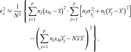 $$\begin{align}{\epsilon}_x^2\approx \frac{1}{N^2}&\left\{\sum \limits_{j=1}^p{n}_j{\left({x}_{hj}-\overline{x}\right)}^2\cdot \sum \limits_{j=1}^p\left[{n}_j{\sigma}_{x_j^{\prime}}^2+{n}_j{\left({\overline{x}}_j^{\prime }-{\overline{x}}^{\prime}\right)}^2\right]\right.\nonumber\\ &\quad\left. -{\left(\sum \limits_{j=1}^p{n}_j{x}_{hj}{\overline{x}}_j^{\prime }-N\overline{x}\kern0.1em {\overline{x}}^{\prime}\right)}^2\right\},\\[-16pt]\nonumber\end{align}$$
where
 $p$
is the number of holes,
$p$
is the number of holes,
 ${x}_{hj}$
is the position of the hole,
${x}_{hj}$
is the position of the hole,
 ${n}_j$
is the number of electrons within the beamlet,
${n}_j$
is the number of electrons within the beamlet,
 $N$
is the total number of electrons,
$N$
is the total number of electrons,
 $\sum \limits_{j=1}^p{n}_j$
,
$\sum \limits_{j=1}^p{n}_j$
,
 $\overline{x}$
is the mean position of all beamlets,
$\overline{x}$
is the mean position of all beamlets,
 ${\overline{x}}_j^{\prime }$
is the mean divergence of the jth beamlet,
${\overline{x}}_j^{\prime }$
is the mean divergence of the jth beamlet,
 ${\overline{x}}^{\prime }$
is the mean divergence of all beamlets and
${\overline{x}}^{\prime }$
is the mean divergence of all beamlets and
 ${\sigma}_{x_j^{\prime }}$
is the mean rms spot size of the jth beamlet at the jth hole.
${\sigma}_{x_j^{\prime }}$
is the mean rms spot size of the jth beamlet at the jth hole.
The mean divergence can be retrieved from the hole and beamlet positions as
 ${\overline{x}}_j^{\prime}=\left({\overline{X}}_j-{x}_{hj}\right)/L$
, where
${\overline{x}}_j^{\prime}=\left({\overline{X}}_j-{x}_{hj}\right)/L$
, where
 $L$
is the distance between the pepper-pot mask and film, and we assume the small angle approximation is valid. The pepper-pot samples only the fraction of the fast electron beam that propagates through the holes in the mask. Thus, the value obtained from this method can only be taken as an approximation of the population.
$L$
is the distance between the pepper-pot mask and film, and we assume the small angle approximation is valid. The pepper-pot samples only the fraction of the fast electron beam that propagates through the holes in the mask. Thus, the value obtained from this method can only be taken as an approximation of the population.
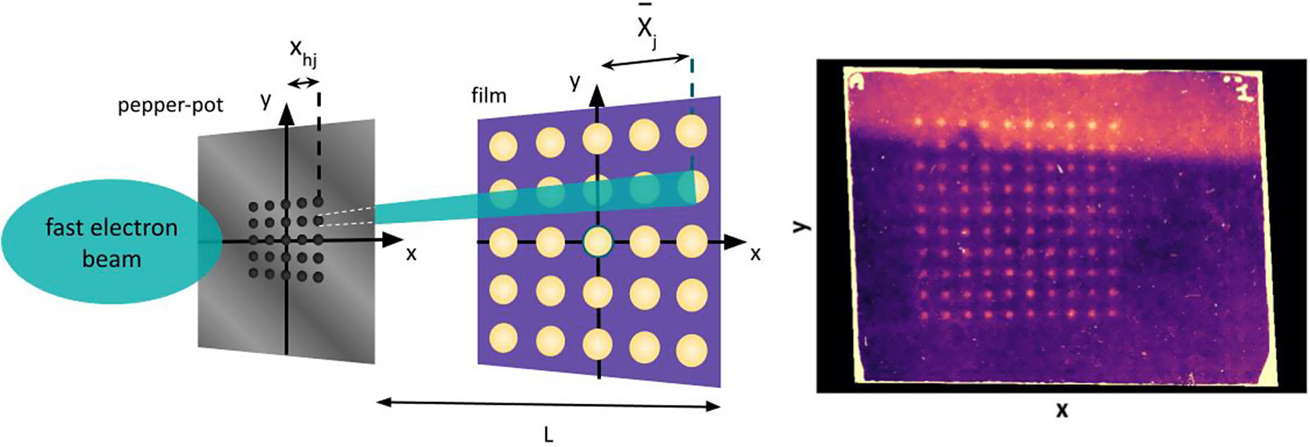
Figure 1 Illustration of the pepper-pot setup. In this configuration the fast electrons propagate from left to right. The image on the far-right shows a sample of the raw data obtained from the experimental work in this paper.
3 Experimental results
The experimental work was conducted at the ILIL facility at INO-CNR, Pisa[
Reference Gizzi, Labate, Baffigi, Brandi, Bussolino, Fulgentini, Köster and Palla35]. The ILIL-PW Ti:sapphire laser line was used to irradiate both planar and NW-coated targets. The NWs were produced via chemical bath deposition[
Reference Calestani, Villani, Cristoforetti, Brandi, Köster, Labate and Gizzi36] onto a
 $5\;\mu \mathrm{m}$
planar Ti substrate, and comprised
$5\;\mu \mathrm{m}$
planar Ti substrate, and comprised
 $6\;\mu \mathrm{m}$
long ZnO wires of average diameter
$6\;\mu \mathrm{m}$
long ZnO wires of average diameter
 $390\pm 50\;\mathrm{nm}$
with an average vacuum gap of
$390\pm 50\;\mathrm{nm}$
with an average vacuum gap of
 $400\pm 200\;\mathrm{nm}$
between the wires. The planar targets were
$400\pm 200\;\mathrm{nm}$
between the wires. The planar targets were
 $12.5\;\mu \mathrm{m}$
thick Ti foil, comparable to the total thickness of the NW targets (
$12.5\;\mu \mathrm{m}$
thick Ti foil, comparable to the total thickness of the NW targets (
 $11\;\mu \mathrm{m}$
).
$11\;\mu \mathrm{m}$
).
An acknowledged concern with the use of nanostructured targets in intense laser interactions is the disruption of the structures by the laser pedestal or pre-pulses prior to the arrival of the main pulse[
Reference Cristoforetti, Anzalone, Baffigi, Bussolino, D’Arrigo, Fulgentini, Giulietti, Köster, Labate, Tudisco and Gizzi37]. The use of a high-contrast laser profile can improve the prospects of retaining the structures until the main pulse interaction. One approach is to frequency double the laser pulse with an appropriate non-linear crystal. In the experiment, second harmonic generation of the 800 nm laser pulse was achieved using a potassium dihydrogen phosphate (KDP) crystal placed immediately after the compressor, creating pulses with a wavelength
 ${\lambda}_{2\omega}\sim 400$
nm. The length of the 800 nm pulse post-compression is 27 fs, which after propagation through the KDP crystal yields a 400 nm pulse with approximate duration of 80 fs FWHM. The laser pulse is reflected off two blue mirrors to remove unconverted 800 nm light and one metallic mirror before striking a silver-coated
${\lambda}_{2\omega}\sim 400$
nm. The length of the 800 nm pulse post-compression is 27 fs, which after propagation through the KDP crystal yields a 400 nm pulse with approximate duration of 80 fs FWHM. The laser pulse is reflected off two blue mirrors to remove unconverted 800 nm light and one metallic mirror before striking a silver-coated
 $f/\sim 4.5$
off-axis parabolic (OAP) mirror, focusing the laser to an elliptical focal spot of size
$f/\sim 4.5$
off-axis parabolic (OAP) mirror, focusing the laser to an elliptical focal spot of size
 $3.5 \;{\mu \mathrm{m}}\times 4.2\;{\mu \mathrm{m}}$
on-target. The laser irradiates the target at an incidence angle of 15°. The frequency doubling process rotates the polarization such that the
$3.5 \;{\mu \mathrm{m}}\times 4.2\;{\mu \mathrm{m}}$
on-target. The laser irradiates the target at an incidence angle of 15°. The frequency doubling process rotates the polarization such that the
 $2\omega$
pulse is s-polarized (E-field oscillation is in the y-direction), as indicated in Figure 2(c). Energy in the pulse at the fundamental frequency,
$2\omega$
pulse is s-polarized (E-field oscillation is in the y-direction), as indicated in Figure 2(c). Energy in the pulse at the fundamental frequency,
 ${\omega}_\mathrm{L}$
, is 5.40 J, with 60% of the energy on-target and 60% of this energy contained within the focal spot. The 2
${\omega}_\mathrm{L}$
, is 5.40 J, with 60% of the energy on-target and 60% of this energy contained within the focal spot. The 2
 ${\omega}_\mathrm{L}$
conversion efficiency is estimated to be approximately 20%, resulting in an estimated energy of 0.4 J in the focal spot. The final intensity on-target is therefore
${\omega}_\mathrm{L}$
conversion efficiency is estimated to be approximately 20%, resulting in an estimated energy of 0.4 J in the focal spot. The final intensity on-target is therefore
 $I\approx 3.9\times {10}^{19}\;\mathrm{W}/{\mathrm{cm}}^2$
.
$I\approx 3.9\times {10}^{19}\;\mathrm{W}/{\mathrm{cm}}^2$
.

Figure 2 (a) Layout of the experimental setup in the vacuum chamber. A pepper-pot diagnostic is placed behind the irradiated target; (b) shows the setup of the pepper-pot. (c) The orientation of the laser fields with respect to the target.
As anticipated, the emittance of the exiting fast electron beam is estimated using a pepper-pot diagnostic setup. Figure 2(a) shows the positioning of the pepper-pot in the target chamber. The pepper-pot mask has a
 $10\times 10$
array of 0.2 mm diameter holes spaced 0.8 mm apart, and is placed at a distance of 17 mm from the rear of the target. An EBT3 film is placed at a distance of 51 mm from the pepper-pot mask to serve as the detector for the sampled fast electrons.
$10\times 10$
array of 0.2 mm diameter holes spaced 0.8 mm apart, and is placed at a distance of 17 mm from the rear of the target. An EBT3 film is placed at a distance of 51 mm from the pepper-pot mask to serve as the detector for the sampled fast electrons.
The emittance formula in Equation (2) is used to calculate a transverse fast electron emittance in x (perpendicular to the laser E-field) and y (parallel) directions from the data obtained from the irradiated planar and NW targets. Each dataset is integrated over two shots for each target type. The dominant error for these measurements is the background correction. The background signal was found to be inhomogeneous, and the upper and lower bounds on each emittance value are taken from analysis cases where the background was taken either above or below the beamlets. Figure 3(a) shows the transverse emittance
 ${\epsilon}_{\perp }$
calculated for each column of measured beamlets from the pepper-pot diagnostic. The fast electrons generated from the laser–NW interaction are generally found to have a larger value of
${\epsilon}_{\perp }$
calculated for each column of measured beamlets from the pepper-pot diagnostic. The fast electrons generated from the laser–NW interaction are generally found to have a larger value of
 ${\epsilon}_{\perp }$
than from the interaction with the planar targets, with average values of
${\epsilon}_{\perp }$
than from the interaction with the planar targets, with average values of
 ${\epsilon}_{\perp}=32\pm 7$
and
${\epsilon}_{\perp}=32\pm 7$
and
 $29\pm 20\;\mathrm{mm}\cdot \mathrm{mrad}$
for the NW and planar targets, respectively. This result of an increased emittance for electrons accelerated from the NW targets is mirrored in the measurements of
$29\pm 20\;\mathrm{mm}\cdot \mathrm{mrad}$
for the NW and planar targets, respectively. This result of an increased emittance for electrons accelerated from the NW targets is mirrored in the measurements of
 ${\epsilon}_{\parallel }$
shown in Figure 3(b). The average values are
${\epsilon}_{\parallel }$
shown in Figure 3(b). The average values are
 ${\epsilon}_{\parallel}=33\pm 10\;\mathrm{mm}\cdot \mathrm{mrad}$
for the NW targets and
${\epsilon}_{\parallel}=33\pm 10\;\mathrm{mm}\cdot \mathrm{mrad}$
for the NW targets and
 ${\epsilon}_{\parallel}=25\pm 8\;\mathrm{mm}\cdot \mathrm{mrad}$
for the planar targets.
${\epsilon}_{\parallel}=25\pm 8\;\mathrm{mm}\cdot \mathrm{mrad}$
for the planar targets.
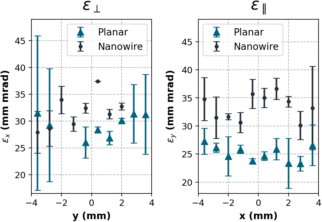
Figure 3 Experimental estimate of the transverse emittance in (a) x, perpendicular to the laser E-field, and (b) y, parallel to the E-field. Error bars are taken from the uncertainty introduced from the background correction applied.
4 Particle-in-cell simulations
Simulations using the PIC code EPOCH[
Reference Arber, Bennett, Brady, Lawrence-Douglas, Ramsay, Sircombe, Gillies, Evans, Schmitz, Bell and Ridgers38] are carried out to explore the laser interaction with the NW and planar targets. A domain is established of size
 $10\;\mu \mathrm{m} \times 12\;\mu \mathrm{m}$
with cells of size
$10\;\mu \mathrm{m} \times 12\;\mu \mathrm{m}$
with cells of size
 $2.5\kern0.24em \mathrm{nm}\times 2.5\;\mathrm{nm}.$
The planar target is modelled as
$2.5\kern0.24em \mathrm{nm}\times 2.5\;\mathrm{nm}.$
The planar target is modelled as
 $8\;\mu \mathrm{m}$
thick Ti at solid density
$8\;\mu \mathrm{m}$
thick Ti at solid density
 ${n}_\mathrm{i}=5.67\times {10}^{29}\ {\mathrm{m}}^{-3}$
. The NW target is composed of Ti wires of diameter and gap size 0.4 μm and length of
${n}_\mathrm{i}=5.67\times {10}^{29}\ {\mathrm{m}}^{-3}$
. The NW target is composed of Ti wires of diameter and gap size 0.4 μm and length of
 $6\;\mu \mathrm{m}$
. The wires are set to half-solid density, and a
$6\;\mu \mathrm{m}$
. The wires are set to half-solid density, and a
 $2\;\mu \mathrm{m}$
thick solid density Ti planar substrate is placed behind the wires. Figures 4(a) and 4(b) show the initial electron density of the planar and NW targets at
$2\;\mu \mathrm{m}$
thick solid density Ti planar substrate is placed behind the wires. Figures 4(a) and 4(b) show the initial electron density of the planar and NW targets at
 $t$
= 0 fs. A reduced target thickness is employed to maintain reasonable computational costs. The focus of the investigation is on the laser–solid interaction at the planar surface and around the wires, which is satisfied without the requirement of a thicker bulk target. An average ionization
$t$
= 0 fs. A reduced target thickness is employed to maintain reasonable computational costs. The focus of the investigation is on the laser–solid interaction at the planar surface and around the wires, which is satisfied without the requirement of a thicker bulk target. An average ionization
 $\overline{Z}$
= 10 is used with the pseudoparticles at an initial temperature of 100 eV. The Ti ion species is represented by 20 pseudoparticles per cell, and the electron species represented by 200 pseudoparticles per cell. Collisions are turned on with ln
$\overline{Z}$
= 10 is used with the pseudoparticles at an initial temperature of 100 eV. The Ti ion species is represented by 20 pseudoparticles per cell, and the electron species represented by 200 pseudoparticles per cell. Collisions are turned on with ln
 $\varLambda$
= 3.
$\varLambda$
= 3.
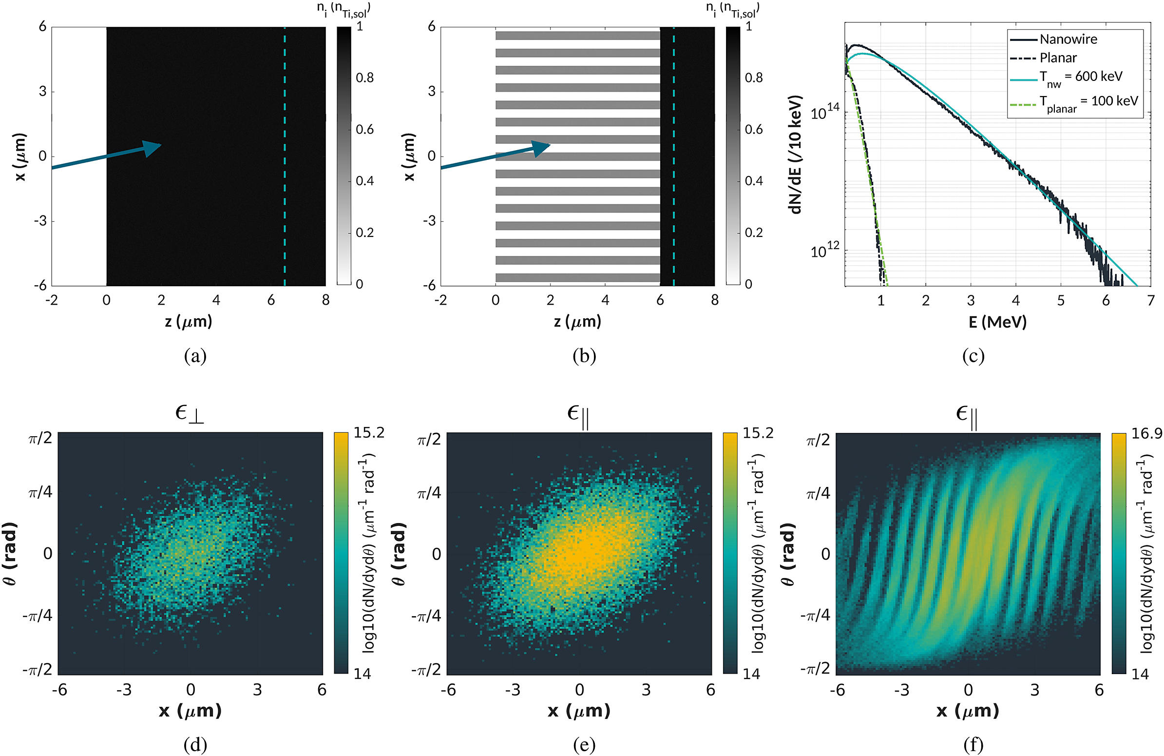
Figure 4 Initial ion density of the (a) planar and (b) nanowire targets modelled in the PIC simulations. The arrow indicates the direction of the incoming laser, irradiating the targets at an angle of 15°. The dashed line indicates the position of the probe plane. The energy spectra of the fast electrons are shown in (c) for the planar and nanowire targets. Plots (d)–(f) show the angular emittance of the fast electrons recorded at the probe plane for the different cases. In (d) the transverse emittance from the s-polarized planar case is shown, which corresponds to the emittance perpendicular to the laser E-field. Plots (e) and (f) show the transverse emittance obtained from the p-polarized interactions with the planar and nanowire targets, respectively. These correspond to the emittance parallel to the laser E-field.
The
 $\lambda$
= 400 nm laser enters the domain from the left-hand side and strikes the target at an incidence angle of 15°. The pulse contains 0.39 J in a Gaussian focal spot of size
$\lambda$
= 400 nm laser enters the domain from the left-hand side and strikes the target at an incidence angle of 15°. The pulse contains 0.39 J in a Gaussian focal spot of size
 ${d}_{\mathrm{FWHM}}=4\;\mu \mathrm{m}$
and a pulse length
${d}_{\mathrm{FWHM}}=4\;\mu \mathrm{m}$
and a pulse length
 ${\tau}_{\mathrm{FWHM}}=80\;\mathrm{fs}$
, corresponding to an on-target intensity
${\tau}_{\mathrm{FWHM}}=80\;\mathrm{fs}$
, corresponding to an on-target intensity
 $I=3.9\times {10}^{19}\;\mathrm{W}/{\mathrm{cm}}^2$
and is turned off at
$I=3.9\times {10}^{19}\;\mathrm{W}/{\mathrm{cm}}^2$
and is turned off at
 $t$
= 100 fs.
$t$
= 100 fs.
In the PIC simulations the laser propagates in the z-direction and the transverse properties of the fast electrons are taken in the x-direction (in two dimensions we cannot explore the y-direction). Therefore, in order to explore both
 ${\epsilon}_{\perp }$
and
${\epsilon}_{\perp }$
and
 ${\epsilon}_{\parallel }$
in a 2D geometry, simulations were performed for both s- and p-laser polarizations. When comparing the results from planar and NW targets the focus is on the p-polarization case. Although the experimental interaction was s-polarized, a clearer difference in emittance measurements between planar and NW targets was observed in the direction parallel to the E-field. This can be explored with the p-polarized 2D simulations.
${\epsilon}_{\parallel }$
in a 2D geometry, simulations were performed for both s- and p-laser polarizations. When comparing the results from planar and NW targets the focus is on the p-polarization case. Although the experimental interaction was s-polarized, a clearer difference in emittance measurements between planar and NW targets was observed in the direction parallel to the E-field. This can be explored with the p-polarized 2D simulations.
4.1 Fast electron properties
A probe plane is placed at
 $z$
= 6.5 μm to collect information on the propagating fast electrons with E
$z$
= 6.5 μm to collect information on the propagating fast electrons with E
 $\ge$
50 keV. Whilst the simulations of the planar and NW targets are performed with a substrate thickness different from the real cases, the electron energy distribution for E
$\ge$
50 keV. Whilst the simulations of the planar and NW targets are performed with a substrate thickness different from the real cases, the electron energy distribution for E
 $>$
50 keV will not be significantly affected by collisions during propagation through these substrate thicknesses. Thus, the probe output can be used as an indicator of the injected fast electron energy spectra. The momentum, p, of each passing electron is used to construct an energy spectrum with bins of 10 keV for the p-polarized simulations. A best fit is found to each spectrum of the form
$>$
50 keV will not be significantly affected by collisions during propagation through these substrate thicknesses. Thus, the probe output can be used as an indicator of the injected fast electron energy spectra. The momentum, p, of each passing electron is used to construct an energy spectrum with bins of 10 keV for the p-polarized simulations. A best fit is found to each spectrum of the form
 $f\left(E,{T}_\mathrm{hot}\right)=\frac{\gamma p}{A}\;\exp \left(-E/{k}_\mathrm{B}{T}_\mathrm{hot}\right)$
, where
$f\left(E,{T}_\mathrm{hot}\right)=\frac{\gamma p}{A}\;\exp \left(-E/{k}_\mathrm{B}{T}_\mathrm{hot}\right)$
, where
 $\gamma$
is the relativistic Lorentz factor,
$\gamma$
is the relativistic Lorentz factor,
 ${T}_\mathrm{hot}$
is the hot electron temperature and A is a normalization constant. A fit is found to the electron spectra from the planar target with a temperature
${T}_\mathrm{hot}$
is the hot electron temperature and A is a normalization constant. A fit is found to the electron spectra from the planar target with a temperature
 ${T}_\mathrm{hot}$
= 100 keV. The hot electron temperatures predicted by the Wilks ponderomotive[
Reference Wilks, Kruer, Tabak and Langdon39] and Sherlock[
Reference Sherlock40] scalings are
${T}_\mathrm{hot}$
= 100 keV. The hot electron temperatures predicted by the Wilks ponderomotive[
Reference Wilks, Kruer, Tabak and Langdon39] and Sherlock[
Reference Sherlock40] scalings are
 ${T}_\mathrm{h}$
= 400 keV and 240 keV, respectively. In comparison, the electron spectra produced from the NW targets can be described by a fit with a temperature
${T}_\mathrm{h}$
= 400 keV and 240 keV, respectively. In comparison, the electron spectra produced from the NW targets can be described by a fit with a temperature
 ${T}_\mathrm{hot}$
= 600 keV, an enhancement relative to the planar target and to the classical hot electron temperature estimates.
${T}_\mathrm{hot}$
= 600 keV, an enhancement relative to the planar target and to the classical hot electron temperature estimates.
An estimate of the emittance of the injected fast electron beams in the planar and NW targets can also be obtained from the diagnostic probe. The crossing position x and angle
 $\theta = \mathrm{arctan}\left({p}_x/{p}_z\right)$
are recorded for each electron passing the probe plane, and are used to generate propagation angle-position plots for the fast electron beam. Figures 4(d) and 4(e) show the angle-position plots from the s-polarized and p-polarized laser–planar interactions, respectively. The p-polarized interaction yields a slightly larger emittance (
$\theta = \mathrm{arctan}\left({p}_x/{p}_z\right)$
are recorded for each electron passing the probe plane, and are used to generate propagation angle-position plots for the fast electron beam. Figures 4(d) and 4(e) show the angle-position plots from the s-polarized and p-polarized laser–planar interactions, respectively. The p-polarized interaction yields a slightly larger emittance (
 ${\epsilon}_y$
) and higher flux of fast electrons than the s-polarized interaction (
${\epsilon}_y$
) and higher flux of fast electrons than the s-polarized interaction (
 ${\epsilon}_x$
). In contrast, the measurements from the pepper-pot suggest the average electron emittance from the planar targets is greater along the direction of the E-field oscillation. However, the uncertainty introduced during analysis results in the estimates of
${\epsilon}_x$
). In contrast, the measurements from the pepper-pot suggest the average electron emittance from the planar targets is greater along the direction of the E-field oscillation. However, the uncertainty introduced during analysis results in the estimates of
 ${\epsilon}_x$
and
${\epsilon}_x$
and
 ${\epsilon}_y$
lying within error of each other and becoming comparable.
${\epsilon}_y$
lying within error of each other and becoming comparable.
A similar emittance plot is constructed for the fast electrons from the NW target. Figure 4(f) shows a highly structured profile with a fraction of the electrons remaining close to the central positions of the wires with a low angular divergence, supporting the argument that the wires can sustain some guiding up to the substrate. The electrons possess a large angular spread from each wire up to
 $\pm \pi /2$
, greater than the angular spread observed from the planar interaction. The plots here reveal a greater overall area in propagation angle-position space is occupied by the fast electrons produced in the NW target, in agreement with the experimental estimate.
$\pm \pi /2$
, greater than the angular spread observed from the planar interaction. The plots here reveal a greater overall area in propagation angle-position space is occupied by the fast electrons produced in the NW target, in agreement with the experimental estimate.
4.2 Electron trajectories
The trajectories of a random subset of individual particles can be extracted from the PIC simulations in order to delve into the influence of the wires on the electron transport. Figure 5(a) shows the trajectories of the highest energy electrons from the p-polarized interaction with the planar target. The electrons are injected at an angle along the laser k-vector direction, indicating we are in a regime where the electrons are primarily heated by ponderomotive acceleration for the planar targets.
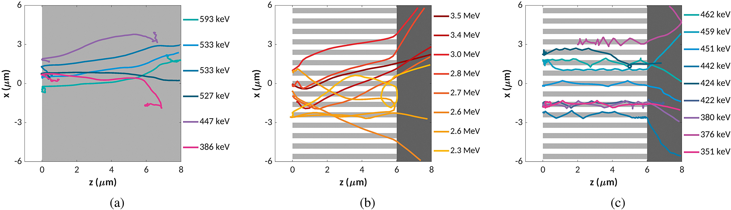
Figure 5 Electron trajectories from a random subset of hot electrons from the p-polarized laser interactions. The electron path is plotted across 120 fs, and is labelled according to the maximum energy reached during the simulation. Figures (a) and (b) show example trajectories of the highest energy electrons for the planar and nanowires respectively, and (c) shows example trajectories of lower energy electrons with
 ${E}_\mathrm{max}\sim$
400 keV from the nanowire interaction.
${E}_\mathrm{max}\sim$
400 keV from the nanowire interaction.
The emittance plot in Figure 4(f) indicates the wires are influencing the transport of the fast electrons. Figure 5(b) shows the paths travelled by electrons heated to a maximum energy
 ${E}_\mathrm{max}>2$
MeV. The electron trajectories are largely unaltered by the neighbouring wires and can propagate across the array. Upon reaching the wire–substrate boundary at
${E}_\mathrm{max}>2$
MeV. The electron trajectories are largely unaltered by the neighbouring wires and can propagate across the array. Upon reaching the wire–substrate boundary at
 $z=6\;\mu \mathrm{m}$
, the paths of some electrons exhibit a deflection, increasing the overall angular extent of the fast electrons as they propagate into the substrate. In contrast, the trajectories of lower energy electrons in Figure 5(c) demonstrate a clear guiding effect of the wires. The electrons are either directed along the wire surface or reflux around the wires, with the effect persisting along the whole length of the wire. Upon reaching the solid substrate this guiding effect is lost and a deflection of the electrons is again observed for some electron trajectories.
$z=6\;\mu \mathrm{m}$
, the paths of some electrons exhibit a deflection, increasing the overall angular extent of the fast electrons as they propagate into the substrate. In contrast, the trajectories of lower energy electrons in Figure 5(c) demonstrate a clear guiding effect of the wires. The electrons are either directed along the wire surface or reflux around the wires, with the effect persisting along the whole length of the wire. Upon reaching the solid substrate this guiding effect is lost and a deflection of the electrons is again observed for some electron trajectories.
4.3 EM field growth
The EM fields around the wires are inspected to explain the trajectories of the fast electrons revealed in the simulations. Figures 6(a) and 6(b) show the evolution of the
 ${E}_x$
and
${E}_x$
and
 ${B}_y$
components around the central wire. In Figure 6(a) at 20 fs there is propagation of the laser fields down the vacuum channels at early times, visible in the region indicated by the dashed lines. Proceeding with the initial laser propagation the field structure is reminiscent of a transverse electromagnetic (TEM) eigenmode, seen in the region selected with the solid rectangle. This can be attributed to the excitation of surface plasmon polaritons (SPPs) at the plasma–vacuum interface[
Reference Macchi41–
Reference Gizzi, Cristoforetti, Baffigi, Brandi, D’Arrigo, Fazzi, Fulgentini, Giove, Köster, Labate, Maero, Palla, Romé, Russo, Terzani and Tomassini43]. At later times a more homogeneous field structure is apparent, orientated along the wire edges.
${B}_y$
components around the central wire. In Figure 6(a) at 20 fs there is propagation of the laser fields down the vacuum channels at early times, visible in the region indicated by the dashed lines. Proceeding with the initial laser propagation the field structure is reminiscent of a transverse electromagnetic (TEM) eigenmode, seen in the region selected with the solid rectangle. This can be attributed to the excitation of surface plasmon polaritons (SPPs) at the plasma–vacuum interface[
Reference Macchi41–
Reference Gizzi, Cristoforetti, Baffigi, Brandi, D’Arrigo, Fazzi, Fulgentini, Giove, Köster, Labate, Maero, Palla, Romé, Russo, Terzani and Tomassini43]. At later times a more homogeneous field structure is apparent, orientated along the wire edges.
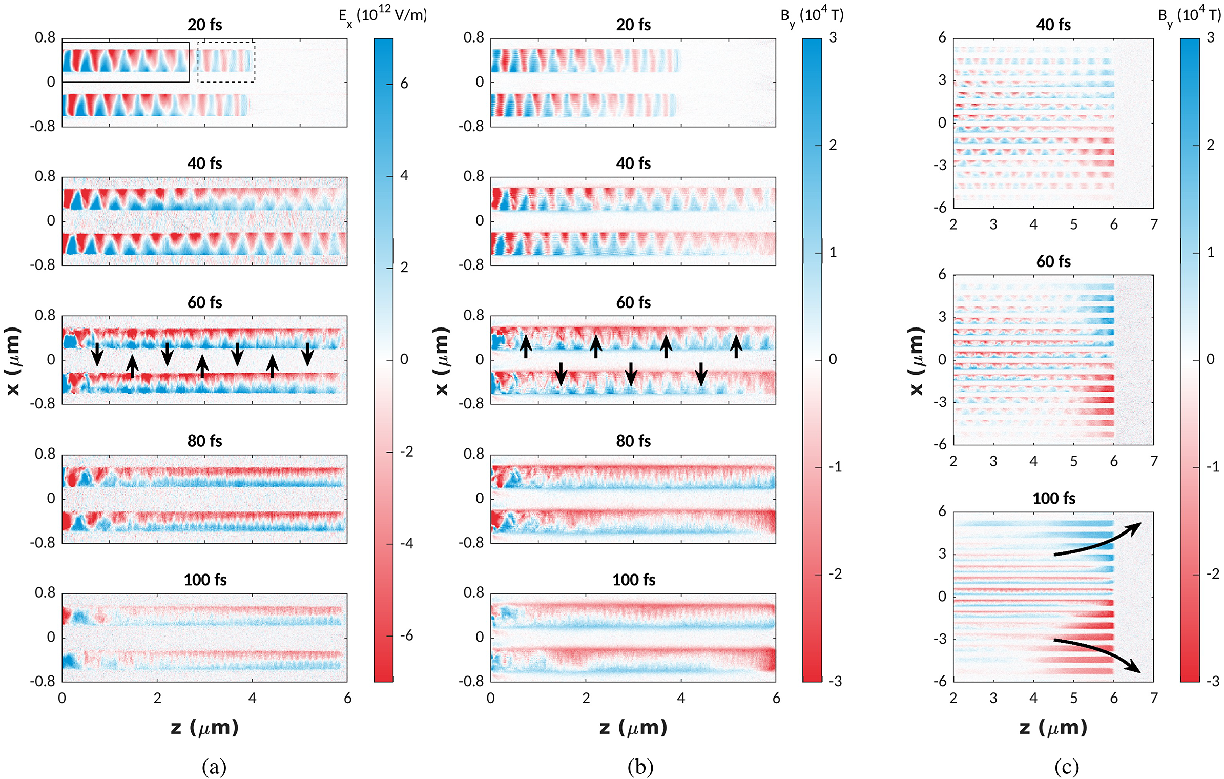
Figure 6 (a) Ex
and (b) By
field components around the central wire for the p-polarized PIC simulation. Black arrows indicate the direction on which the fields will act on an electron propagating in the z-direction. The By
field is shown in (c) across the whole target. The black arrows here indicate the direction of deflection of an electron propagating in the
 ${+}z$
-direction.
${+}z$
-direction.
In addition to the ‘local’ fields around a single wire, it can be instructive to also look at the ‘global’ fields across the larger simulation domain. Figure 6(c) shows the
 ${B}_y$
component across all wires and the substrate. As early as 40 fs we are able to identify the growth of an azimuthal magnetic field at the wire–substrate boundary, which continues to grow in strength over the laser pulse time of 100 fs. Chatterjee et al. [
Reference Chatterjee, Singh, Ahmed, Robinson, Lad, Mondal, Narayanan, Srivastava, Koratkar, Pasley, Sood and Kumar44] previously reported the growth of strong self-generated magnetic fields at the rear target–vacuum boundary from fs-interactions with nanochannel targets; our simulations suggest these azimuthal fields can additionally grow to kT-levels at the wire–substrate interface.
${B}_y$
component across all wires and the substrate. As early as 40 fs we are able to identify the growth of an azimuthal magnetic field at the wire–substrate boundary, which continues to grow in strength over the laser pulse time of 100 fs. Chatterjee et al. [
Reference Chatterjee, Singh, Ahmed, Robinson, Lad, Mondal, Narayanan, Srivastava, Koratkar, Pasley, Sood and Kumar44] previously reported the growth of strong self-generated magnetic fields at the rear target–vacuum boundary from fs-interactions with nanochannel targets; our simulations suggest these azimuthal fields can additionally grow to kT-levels at the wire–substrate interface.
5 Discussion
PIC simulations have revealed the evolution of strong electric and magnetic fields around the wires that affect the fast electron transport. At early times the fields inside the NW channels due to laser propagation and SPP excitation can extract and accelerate electrons from the wires[ Reference Zou, Yu, Jiang, Yu, Chen, Zhuo, Zhou and Ruan45]. At later times a prominent quasistatic field structure is instead evident. As the electrons are extracted from the wires, a charge separation will be established between the wire and vacuum regions. This will result in the generation of an electrostatic Ex field between the wires.
Figure 7(a) shows the averaged current densities along the wires at a time
 $t$
= 80 fs. There is a net negative current density in the vacuum gaps, corresponding to electrons propagating in the +
$t$
= 80 fs. There is a net negative current density in the vacuum gaps, corresponding to electrons propagating in the +
 $z$
-direction towards the substrate. This is neutralized within the wires due to the drawing of a return current. A net positive current is observed at the wire edges. The current density gradient between the wire and the vacuum could therefore explain the B-field growth observed in the simulations. Previous works have identified the drawing of the return current down the wires as the primary source of azimuthal B-field growth at the wires[
Reference Ji, Jiang, Wu, Wang, Gu and Tang46–
Reference Fedeli, Formenti, Cialfi, Pazzaglia and Passoni48].
$z$
-direction towards the substrate. This is neutralized within the wires due to the drawing of a return current. A net positive current is observed at the wire edges. The current density gradient between the wire and the vacuum could therefore explain the B-field growth observed in the simulations. Previous works have identified the drawing of the return current down the wires as the primary source of azimuthal B-field growth at the wires[
Reference Ji, Jiang, Wu, Wang, Gu and Tang46–
Reference Fedeli, Formenti, Cialfi, Pazzaglia and Passoni48].
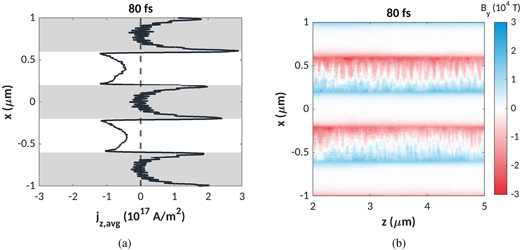
Figure 7 (a) Current density
 ${j}_z$
averaged in the range z = 2–5 μm. Shaded regions indicate the wire positions and the white regions indicate vacuum. (b) Corresponding
${j}_z$
averaged in the range z = 2–5 μm. Shaded regions indicate the wire positions and the white regions indicate vacuum. (b) Corresponding
 ${B}_y$
fields (orthogonal to the simulation plane) within the same region.
${B}_y$
fields (orthogonal to the simulation plane) within the same region.
For an electron propagating along a wire in z, the
 ${B}_y$
field will act to expel the electron from the wire, whereas the
${B}_y$
field will act to expel the electron from the wire, whereas the
 ${E}_x$
field will draw the electron back in. This will result in a ‘push–pull’ net effect on an individual electron[
Reference Ji, Jiang, Wu, Wang, Gu and Tang46,
Reference Wang, Zhao, He, Cao, Dong, Wu, Zhu, Zhang, Zhang, Zhang and Gu49]. Figure 8 evidences the effect of the guiding fields around the wires on high- and low-energy electrons as they propagate across the wire array. For a lower energy electron with
${E}_x$
field will draw the electron back in. This will result in a ‘push–pull’ net effect on an individual electron[
Reference Ji, Jiang, Wu, Wang, Gu and Tang46,
Reference Wang, Zhao, He, Cao, Dong, Wu, Zhu, Zhang, Zhang, Zhang and Gu49]. Figure 8 evidences the effect of the guiding fields around the wires on high- and low-energy electrons as they propagate across the wire array. For a lower energy electron with
 ${E}_{\mathrm{max}}$
= 400 keV, the fields are sufficiently strong to reduce the transverse momenta to the opposite sign and effectively restrict the electron trajectory around the wire and guide it. A higher energy electron with
${E}_{\mathrm{max}}$
= 400 keV, the fields are sufficiently strong to reduce the transverse momenta to the opposite sign and effectively restrict the electron trajectory around the wire and guide it. A higher energy electron with
 ${E}_{\mathrm{max}}$
= 3 MeV experiences a similar modulation in the transverse momenta. However, the initial
${E}_{\mathrm{max}}$
= 3 MeV experiences a similar modulation in the transverse momenta. However, the initial
 ${p}_x$
is great enough that the change in momenta does not affect the overall trajectory significantly. The electron continues to propagate in the +x-direction across the wire array and does not exhibit a clear guiding along a wire structure.
${p}_x$
is great enough that the change in momenta does not affect the overall trajectory significantly. The electron continues to propagate in the +x-direction across the wire array and does not exhibit a clear guiding along a wire structure.
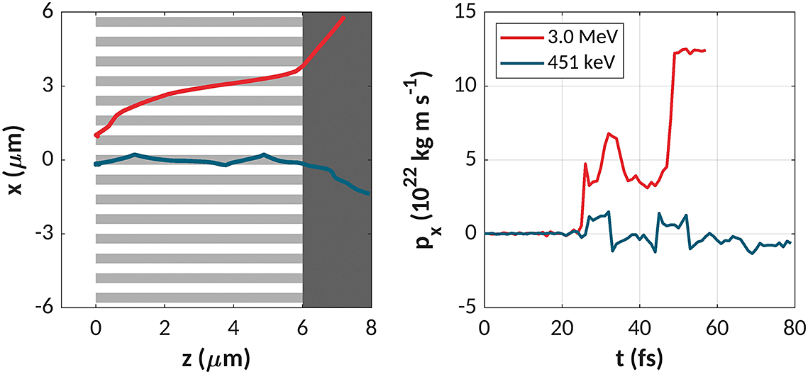
Figure 8 The transverse momenta of two example fast electrons as they traverse the wire region. The blue trajectory is for an electron with a final energy close to the ponderomotive temperature, and the red trajectory is for one of the highest energy MeV electrons.
Whilst evidence has been presented here demonstrating the ability of the NWs to guide the electrons under particular conditions, the geometry is clearly not optimized to reduce the final emittance. Many electrons undergo an oscillatory motion around the wires and their transverse momenta are hardly reduced by the NW structures, and are even enhanced compared to planar targets, as shown in Figures 4(e) and 4(f). Since the fields responsible for inducing the oscillatory nature of the fast electron transport are a consequence of extracting and accelerating the electrons from the wires, it may be difficult to avoid this entirely.
The larger azimuthal magnetic field at the wire–substrate boundary has been explored and identified elsewhere in intense laser interactions with planar targets[
Reference Gizzi, Mackinnon, Riley, Viana and Willi50–
Reference Nakatsutsumi, Sentoku, Korzhimanov, Chen, Buffechoux, Kon, Atherton, Audebert, Geissel, Hurd, Kimmel, Rambo, Schollmeier, Schwarz, Starodubtsev, Gremillet, Kodama and Fuchs53], primarily on the effect on sheath-accelerated protons at the rear surface. These self-generated magnetic fields at the front surface of the target can be attributed to the ‘fountain effect’[
Reference Sakagami, Kawakami, Nagao and Yamanaka54–
Reference Pukhov56] arising from the interplay between the counter-propagating injected fast electron and return currents. Fast electrons propagating through the +
 ${B}_y$
region (blue) will be deflected upwards in the x direction, and those propagating through the –
${B}_y$
region (blue) will be deflected upwards in the x direction, and those propagating through the –
 ${B}_y$
region (red) will be deflected downwards in the –x direction. This is in agreement with the observed electron trajectory deflections in Figures 5(b) and 5(c).
${B}_y$
region (red) will be deflected downwards in the –x direction. This is in agreement with the observed electron trajectory deflections in Figures 5(b) and 5(c).
A consideration of these generated fields is vital for full exploitation of the wires as fast electron guiding elements. A mitigation of the defocusing magnetic field growth at the wire–substrate interface could be realized through proper choice of laser-target parameters. For example, since the strength of the magnetic field generated scales with the injected fast electron current density[ Reference Schumaker, Nakanii, McGuffey, Zulick, Chyvkov, Dollar, Habara, Kalintchenko, Maksimchuk, Tanaka, Thomas, Yanovsky and Krushelnick57], a larger focal spot could be implemented to reduce the deflection experienced by the fast electrons accelerated in the wires. In addition, lower energy electrons appear to be more readily guided along the wires and suffer less deflection due to the B-field at the substrate.
Finally, we note that the 2D simulations of NW targets are inherently inaccurate to reproduce the target geometry since they model infinite ‘slabs’ in the y-direction. Simulation studies by Fedeli et al. [ Reference Fedeli, Formenti, Cialfi, Pazzaglia and Passoni48] and Jiang et al. [ Reference Jiang, Krygier, Schumacher, Akli and Freeman31] compared the effectiveness of 2D simulations as a means of reproducing three-dimensional (3D) simulations. Whilst the qualitative results could be reproduced, there were differences observed in the final laser absorption and electron temperatures. However, the EM fields between the wire gaps should be reliably reproduced in two dimensions for this wire diameter and spacing, as should the transverse guiding of the electrons. In addition, the generation of the azimuthal B-field at the substrate can still be captured in two dimensions.
6 Conclusion
NW targets are frequently endorsed as a means to attain higher laser absorption into fast electrons. Enhanced coupling into fast electrons, resulting in an increased electron flux or temperature, is well-recognized, as is the potential for the wires to guide the electrons. Less attention has been paid to the transport of the electrons as they exit the influence of the wires and the effect of the wires on the overall electron beam properties. The experimental measurements reported here suggest an increased emittance of the escaping fast electron beam from the NW targets. PIC simulations explain this increase in emittance not only by an increased hot electron temperature, but also through the discovery of a self-generated magnetic field growing at the wire–substrate boundary that serves to defocus the electron beam. Further work on the use of NW targets as an efficient fast electron beam source should consider this field generation carefully. The detrimental effects on the beam emittance could be reduced by employing appropriate wire geometries and laser parameters.
Acknowledgements
We acknowledge financial support from the NextGenerationEU (PNRR) Integrated Infrastructure Initiative in Photonic and Quantum Sciences (IPHOQS) (CUP B53C22001750006, ID D2B8D520, IR0000016) and EuPRAXIA Advanced Photon Sources (EuAPS) (CUP I93C21000160006, IR0000030). We also acknowledge support and funding from the Engineering and Physical Sciences Research Council (EP/L01663X/1) and the Royal Society International Exchange (IES/R3/170248). Computing resources were provided by STFC Scientific Computing Department’s SCARF cluster. This work was in part funded by the UK EPSRC (grants EP/G054950/1, EP/G056803/1, EP/G055165/1 and EP/ M022463/1).


 Open access