1. Introduction
Historically, dominance has often been ignored or treated as a nuisance parameter, for example in genetic evaluations of livestock and quantification of variance components (VCs). The importance of detection and quantification of dominance effects underlying complex traits, however, is underlined by an increasing body of evidence for dominant quantitative trait locus (QTL) with major effects on human disease and agricultural traits of economic importance. Duong et al. (Reference Duong, Charron, Xiao, Hamet, Menard, Roy and Deng2006) found eight completely dominant QTL associated with hypertension in congenic rat lines, and in agriculture, examples of dominant QTL include fertility and production traits in cattle (Cohen-Zinder et al., Reference Cohen-Zinder, Seroussi, Larkin, Loor, Everts-Van Der Wind, Lee, Drackley, Band, Hernandez, Shani, Lewin, Weller and Ron2005), chicken (Ikeobi et al., Reference Ikeobi, Woolliams, Morrice, Law, Windsor, Burt and Hocking2002; Hocking, Reference Hocking2005), tomatoes (Semel et al., Reference Semel, Nissenbaum, Menda, Zinder, Krieger, Issman, Pleban, Lippman, Gur and Zamir2006) and maize (Zhang et al., Reference Zhang, Zhao, Ding, Rong and Pan2006). Liu et al. (Reference Liu, Jennen, Tholen, Juengst, Kleinwachter, Holker, Tesfaye, Un, Schreinemachers, Murani, Ponsuksili, Kim, Schellander and Wimmers2007) performed a genome-wide scan on an F2 Duroc×Pietrain cross and found 40 additive QTL and 31 QTL showing overdominance effects. Although definitions vary, overdominance is a phenomenon for which there is increasing evidence in plants as the underlying mechanism for heterosis (Xiao et al., Reference Xiao, Li, Yuan and Tanksley1995; Frascaroli et al., Reference Frascaroli, Cane, Landi, Pea, Gianfranceschi, Villa, Morgante and Pe2007). Lippman & Zamir (Reference Lippman and Zamir2007) review detection and characterization of heterosis, overdominance and pseudo-overdominance.
To date, the detection of these dominant QTL effects has predominantly involved model species or experimental crosses requiring inbred or genetically divergent populations. Reproductive constraints render these test crosses impractical for many agricultural species, while for human and natural populations they are unethical and/or untenable. In commercial livestock populations, it is often more relevant, practical and cost-effective to explore QTL segregating within a population, particularly if the objective is to facilitate selection within that population. There is evidence to suggest that much of the variation found between lines is segregating within lines (De Koning et al., Reference De Koning, Haley, Windsor, Hocking, Griffin, Morris, Vincent and Burt2004) and, furthermore, most evolutionarily important variation appears to occur within lines (Erickson et al., Reference Erickson, Fenster, Stenoien and Price2004).
There is, therefore, an increasing need for QTL methodology to routinely account for genetic interactions such as dominance within any population structure. Independently developed within human and livestock research, VC-based linkage methods (Fernando & Grossman, Reference Fernando and Grossman1989; Goldgar, Reference Goldgar1990; Amos, Reference Amos1994; Grignola et al., Reference Grignola, Zhang and Hoeschele1997; Almasy & Blangero, Reference Almasy and Blangero1998; Allison et al., Reference Allison, Neale, Zannolli, Schork, Amos and Blangero1999; George et al., Reference George, Visscher and Haley2000) have the advantage of simultaneously locating and estimating genetic effects within arbitrary pedigrees. Genetic parameters associated with the polygenic effect, and at specific loci using marker and pedigree information, can be estimated simultaneously. The incorporation of many alleles or allelic effects and all relationships within a pedigree has been shown to increase the power to detect QTL over sib-based methods (Williams & Blangero, Reference Williams and Blangero1999; Sham et al., Reference Sham, Cherny, Purcell and Hewitt2000; Kolbehdari et al., Reference Kolbehdari, Jansen, Schaeffer and Allen2005; Rowe et al., Reference Rowe, Windsor, Haley, Burt, Hocking, Griffin, Vincent and De Koning2006). Furthermore, linkage disequilibrium and haplotype information can be incorporated to provide greater accuracy (Meuwissen et al., Reference Meuwissen, Karlsen, Lien, Olsaker and Goddard2002; Lee & Van der Werf, Reference Lee and Van der Werf2006). Most importantly, there is the potential for flexibility to incorporate random effects and their interactions, for example, dominance, epistasis and maternal effects, limited only by the size and structure of the experimental population.
Although undeniably an important source of variation, non-additive effects are notoriously difficult to estimate due to confounding with other sources such as common maternal environment (Gengler et al., Reference Gengler, Van Vleck, MacNeil, Misztal and Pariacote1997; Misztal, Reference Misztal1997). Computational complexity combined with the more generic problems of setting appropriate thresholds to account for multiple testing and lack of suitable data have inhibited the extension of VC methodology to incorporate interactions such as dominance and epistasis. Although extensions to VC QTL linkage models to incorporate dominance are widely discussed (Sham et al., Reference Sham, Cherny, Purcell and Hewitt2000; Diao & Lin, Reference Diao and Lin2005), they have rarely been implemented, indicating a need for further investigation before the full potential of these methods can be unleashed.
In the present study, extensive simulations have been used to explore the power and potential for partitioning QTL effects into additive and dominant components using VC methods for linkage analysis. Varying full-sib and half-sib population structures have been used to evaluate accuracy and the power to detect additive and dominant genetic effects in pedigrees that are representative of commercial livestock and human scenarios.
2. Materials and methods
(i) Statistical genetic models for VC analysis
Population-wide linkage equilibrium between QTL and marker alleles was assumed for all analyses. Following the two-step approach described by George et al. (Reference George, Visscher and Haley2000), for each putative QTL position, marker information was used to estimate identity-by-descent (IBD) coefficients for all relationships in the pedigree. In the second step, different QTL models were fitted for given genome locations using the following models:
where y is a vector of phenotypic observations, β is a vector of fixed effects, u, a, d, m and e are vectors of random additive polygenic effects, additive and dominance QTL effects at the putative QTL position, non-genetic maternal effects and residuals, respectively, and X, Z and W are incidence matrices relating to records of fixed and random genetic and maternal effects, respectively.
Variances for polygenic and QTL effects are distributed as follows: Var(a)=Gσ2q, Var(d)=Dσ2d, var(e)=Iσ2e and var(u)=Aσ2a. For the non-genetic maternal effect: Var(m)=Iσ2m.
Here, A is the standard additive relationship matrix based on pedigree data only, G is the QTL additive genetic relationship matrix based on marker information and D is the QTL dominance genetic relationship matrix representing the probability that two individuals have the same pair of alleles in common based on marker information. VCs for each model were estimated using REML (Patterson & Thompson, Reference Patterson and Thompson1971) implemented in the ASReml package (Gilmour et al., Reference Gilmour, Thompson and Cullis1995).
(ii) Calculating the relationship matrices A, G and D needed for the mixed model analysis
The relationship matrices G and D for a given QTL position are calculated from the gametic IBD matrix as outlined by Liu et al. (Reference Liu, Jennen, Tholen, Juengst, Kleinwachter, Holker, Tesfaye, Un, Schreinemachers, Murani, Ponsuksili, Kim, Schellander and Wimmers2002). The gametic IBD matrix is a 2n×2n matrix containing the probability of identity of descent between either of the two gametes of an individual with the gametes of the remaining individuals in the pedigree. In contrast to George et al. (Reference George, Visscher and Haley2000), who used a Monte Carlo method, the gametic IBD matrix was estimated with the recursive method of Pong-Wong et al. (Reference Pong-Wong, George, Woolliams and Haley2001), which uses the two first-available fully informative or phase-known flanking markers. The G and D matrices are conditional on flanking marker information and therefore unique for each position evaluated for a QTL; hence, the calculation of G and D requires the prior calculation of the gametic IBD matrix conditional on linked marker information at the position of the putative QTL. Here, the matrices were calculated every 5 cM. In order to estimate the VCs for the different models, ASReml requires the inverse of the relationship matrices A, G and D. The version of ASReml used calculates the inverse of the A matrix directly from pedigree data, but the inverse for G and D were calculated from the gametic matrix, inverted using a separate routine and then passed into ASReml.
(iii) Test statistic
A test statistic for a given location was obtained by comparing the likelihood of the full vs. the null model. The log likelihood-ratio test (LRT) statistic was calculated as twice the difference between the log likelihood of the full model and the reduced model. Power was estimated both empirically using thresholds derived from 1000 chromosome-wise replicates, and using tabulated values assuming that the test statistic is χ2 distributed with degrees of freedom equal to the number of extra parameters estimated in the full model compared with the reduced model. This is conservative for a test at a single location in the genome as the test statistic under the null hypothesis is likely to be distributed as a complex mixture of distributions (Self & Liang, Reference Self and Liang1987; Stram & Lee, Reference Stram and Lee1994; Allison et al., Reference Allison, Neale, Zannolli, Schork, Amos and Blangero1999; Visscher, Reference Visscher2006). For QTL mapping, it has been suggested that the most straightforward method of achieving the critical null value is to halve the P value obtained for χ2k, where k is the number of extra VCs in the full model (Visscher, Reference Visscher2006). In practice, this mixture of distributions χ20−1 is equal to using the 10% critical threshold for a 5% type 1 error rate.
Three tests were carried out: (i) additive QTL (2) vs. null (1) to test significance of the QTL VC under a purely additive model (denoted 1v0); (ii) additive QTL+dominance QTL (3) vs. null (1) to test significance of QTL VCs under a model including additive and dominance effects (denoted 2v0); and (iii) additive QTL+dominance QTL (3) vs. additive QTL (2) to test the significance of the dominance VC (denoted 2v1). To estimate the effect of common environment, the model including additive and dominance QTL effects was further extended to incorporate a random dam effect (4), representing a maternal or full-sib family effect.
(iv) Population structure
The method was implemented in three simulated populations, representative of poultry, pig and human pedigrees (Table 1). The parental generation was simulated by random sampling without replacement from an unrelated base population. Under each scenario, random mating of parents was simulated to obtain a second generation of 1900 progeny.
Table 1. Population parameters for simulated pedigrees
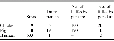
A 20 cM chromosome was simulated with five markers spaced at 5 cM intervals and a bi-allelic QTL between the second and third markers at 7·5 cM. To simulate polygenic variance, ten unlinked additive effects of 0·2 were simulated each with an allele frequency of 0·5 following Alfonso & Haley (Reference Alfonso and Haley1998). The phenotypes generated under a polygenic model were normally distributed, indicating that these unlinked QTL were sufficient to provide a reasonably structured polygenic variance.
Dominance effects were simulated ranging from partial to overdominance over a range of additive effects. These are summarized in Table 2. The variances of the QTL additive (a) and dominance (d) effects were calculated as 0·5 a 2 and 0·25d 2, respectively, because allele frequencies were set to 0·5.
Table 2. Summary of scenarios
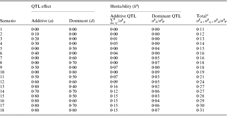
σ2P is the phenotypic variance.
a Total heritability includes polygenic variance (σ2a) of 0·2, residual variance 0·75, expected additive QTL variance (σ2q) estimated by (a 2/2) and expected dominant QTL variance (σ2d) estimated by (d 2/4).
For each individual, a residual effect was sampled from a normal distribution with mean 0 and a variance of 1·5. As the error variance was constant, phenotypic variance and overall heritability increased with genetic effects. In the base scenario with no QTL simulated, polygenic heritability was 0·11. Total heritability (polygenic and QTL) ranged from 0·1 to 0·31 with dominance QTL effects ranging from 0 to 9% of the phenotypic variance. For each scenario where QTL were simulated, 100 replicates were analysed and the test statistics described above calculated at 2, 7, 12 and 17 cM.
(v) Maternal effect
Common environment or direct maternal effects are often, at least partially, confounded with dominance. To explore the effect on detection of dominance QTL, random maternal effects were simulated in the pig population. A maternal effect was simulated by sampling for each full-sib family from a normal distribution with variance of 0·1 and assigning this value to each full-sib offspring. A residual effect was sampled from a normal distribution with mean 0 and a variance of 0·75. The implication of potential maternal effects was evaluated in three different ways: a maternal effect was simulated with a range of dominance QTL effects. Firstly, the maternal effect was not fitted in the model to test for spurious detection of dominance. Secondly, a maternal effect was included in the linear model to test whether the model correctly accounts for the maternal variance. Finally, no maternal effect was simulated but a maternal component was included in the linear model to test whether the dominance variance was correctly identified or incorrectly estimated as a maternal effect.
(vi) Null distribution
Chromosome-wise type 1 error rates were determined empirically for all three population structures. A total of 1000 replicates were used to explore 1, 5 and 10% thresholds under the null scenario (both additive and dominance QTL effects set to zero). Point-wise test statistics were determined with 1000 replicates at the QTL position. Empirical distributions for point-wise tests were compared with tabulated values for χ2k, where k is equal to the number of extra VCs estimated using P values for 1, 5 and 10%, and under the assumption that halving the P value accounts for a mixture of distributions using P values of 2, 10 and 20% for 1, 5 and 10% thresholds. A 5% threshold was determined for empirical power calculations and comparisons based on the analysis of 1000 replicates.
The empirical distribution of the LRT under the null scenario appeared to vary across pedigrees, in particular, differing between human and livestock. This could be due to the difference in number of full sibs per family (three for humans compared with 10 or 20 for livestock) or the lack of half-sib relationships in the human pedigree. To explore this, chromosome-wise null LRT distributions were determined for five additional pedigrees. The number of offspring remained constant at 1900 but pedigrees with 1 or 2 dams per sire and 3, 5 or 10 offspring per dam were compared with pig and poultry pedigrees to explore the effects of family structure on the distribution of the null test statistic.
3. Results
All results shown are based on 5% empirical thresholds from 1000 chromosome-wise replicates. Full results for all populations and scenarios can be found in Supplementary Table S1 for power to detect additive and dominant QTL effects, S2 for power in pig populations with maternal or common environment effects and S3 for estimates of VCs.
(i) Power to detect dominance effects
Figures 1a, b and c give the proportion of replicates detecting dominance using 5% empirical and tabulated thresholds for χ21 and a mixture χ21−0. Testing for dominance involved comparing the additive QTL model with the full model incorporating both an additive QTL and a dominant QTL effect (denoted 2v1). For the pig and poultry pedigrees, power under empirical and the χ21−0 mixture of distributions was in close agreement. For human pedigrees, both χ21 and χ21−0 were conservative when compared with empirical thresholds. Power under the empirical 5% threshold was ~100% in the poultry scenario, ~84% for the pig scenario and ~42% for humans when the QTL dominance variance was about 7% of the phenotypic variance (dominant effect=0·8, i.e. complete dominance). Under χ21 thresholds this dropped to ~95, ~75 and ~25. Power to detect dominance was greater for all pedigrees using empirical thresholds. Although the ranking did not change when using tabulated values, power to detect dominance, particularly in humans, was much lower and differences between models greater. When comparing the full model with the null model (denoted 2v0), all replicates detected a QTL for the pig and poultry scenarios, and 96% (84% under tabulated thresholds) of replicates detected a QTL for the human scenario (Supplementary Table S1).
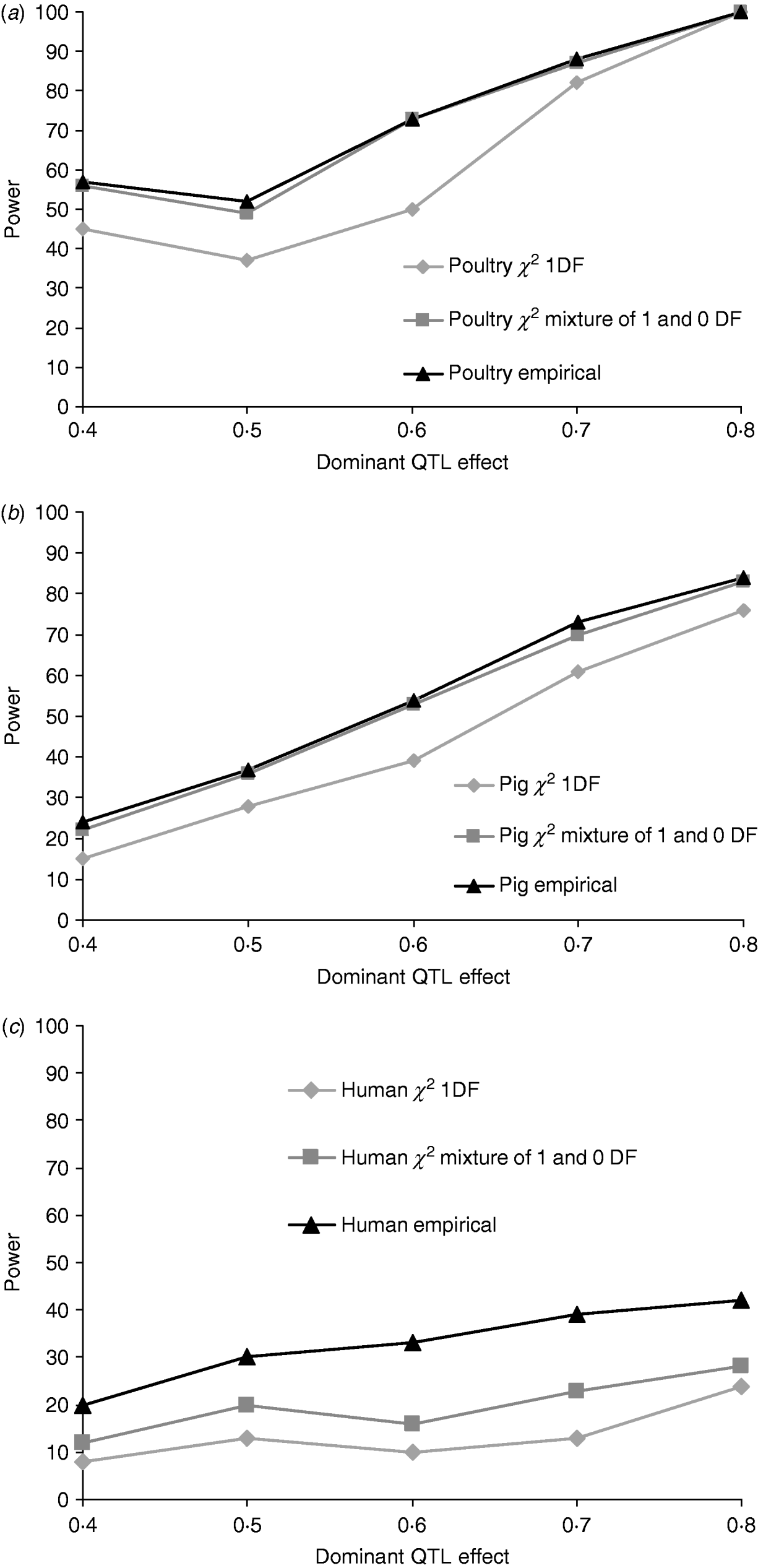
Fig. 1. Proportion of replicates where test for dominance (2v1) is significant (P<0·05) when comparing the full model and the additive model. A total of 100 chromosome-wise replicates in (top to bottom) (a) poultry, (b) pig and (c) human pedigrees under partial to complete dominance. Simulated additive effect fixed at 0·8 comparing tabulated 5% χ21, χ21−0 thresholds and 5% empirical threshold. Mixture threshold is estimated by using tabulated 10% χ21 threshold.
Figure 2 shows the estimates for the additive and dominance QTL VCs from the comparison of the full model with the null model (2v0). In all replicates, a QTL was detected at the 5% significance level. Scenarios shown were for complete dominance with effects ranging from 0·5 to 0·8 (also given in Supplementary Table S2). These show that although estimates are wide-ranging, they appear to accurately estimate the mean.
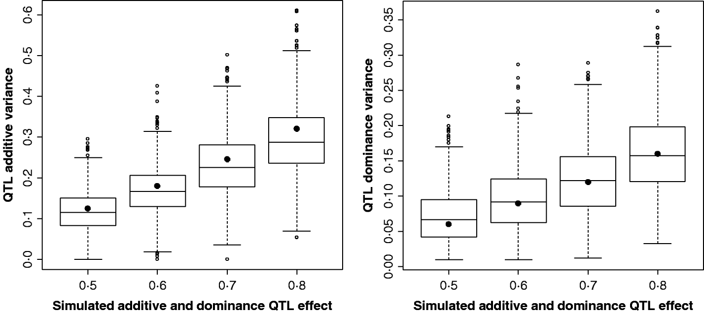
Fig. 2. Estimates of VCs from simulated poultry data. Box plots showing the range of variance estimates. Full dominance is simulated. Variance estimates for single marker position (for 1000 replicates of each scenario) for additive and dominant QTL effects. The black circles indicate the expected VCs. All replicates were significant for a QTL when testing under the full model (additive and dominance QTL effects vs. null).
(ii) Overdominant, spurious additive and dominant QTL effects
Figure 3 shows power to detect simulated additive effects ranging from 0·1 to 0·5, or 1–7% of phenotypic variance. Power reached 90% when the additive variance amounted to >4% of the phenotypic variance. In this case, no dominance effect was simulated and there was little spurious dominance detected. Furthermore, power to detect an additive effect was similar whether or not the extra dominance component was included in the analysis. This shows that a routine scan including dominance would not result in too great a loss of power even in the absence of any dominant effects. Although results are shown only for the pig population, the same pattern was seen for poultry and human scenarios. Figure 4, however, shows that spurious additive QTL effects were found when dominant QTL effects were not fitted. With dominant QTL effects ranging from 0·5 to 0·8 and simulated additive effects of zero, i.e. overdominance, there is both spurious detection of an additive QTL effect if dominance was not included in the model and inflated estimates of additive variance (Table 3).

Fig. 3. Percentage of replicates detecting additive QTL effects (P<0·05) using the full model (add+dom) and the additive model (add) and testing the difference between the two (dom) in a simulated pig population. A dominance effect of zero is simulated.

Fig. 4. Overdominance: percentage of replicates detecting overdominant QTL effects (P<0·05) using the full model (add+dom) and the additive model (add) and testing the difference between the two (dom) in a simulated poultry population over a range of dominant QTL effects when an additive effect of zero is simulated.
Table 3. Estimates of variance due to additive QTL and additive and dominant QTL effects under overdominance when the additive QTL effect of zero is simulated
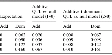
Variances are mean estimates at the highest chromosome-wise test statistic across 100 iterations in a simulated pig population.
(iii) Maternal effects and dominance in the pig scenario
Figure 5 clearly shows that a simulated maternal effect can masquerade as a dominant QTL effect. In the most extreme case when a dominance effect of 0 was simulated, ignoring the common environment resulted in a type 1 error of 67%. When a maternal effect was fitted in the model, maternal effects and dominance appear to be successfully separated with little or no loss of power (Table 4). If a maternal effect was fitted when not present, there was little loss of power (for results see supplementary Tables S2 and S3), indicating that a maternal component fitted in the absence of a maternal effect should not prevent detection of variance due to dominance.
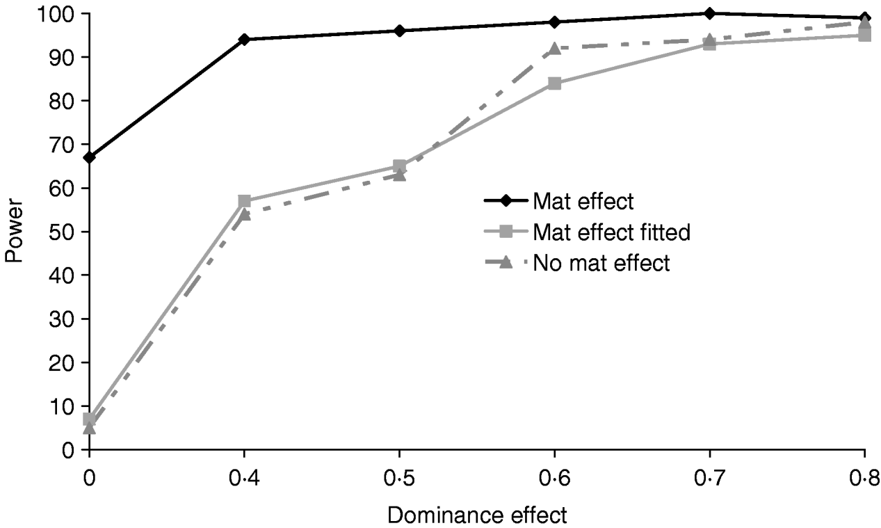
Fig. 5. Effects of simulating and/or fitting direct maternal effects on proportion of replicates where test for dominance (2v1) is significant (P<0·05) when comparing the full model and the additive model. A total of 100 chromosome-wise replicates in the pig population under partial to complete dominance (additive QTL effect fixed at 0·8). ‘No mat effect’, no maternal effect simulated or fitted; ‘mat effect’, maternal variance of 0·1 simulated but not fitted; ‘mat effect fitted’, maternal variance of 0·1 simulated and fitted.
Table 4. Variance estimates for dominant QTL effect of 0·8 and maternal effects

Values in parentheses are simulated or expected variances. Variances are mean estimates at the highest chromosome-wise test statistic across 100 iterations in a simulated pig population.
(iv) Null distribution
Table 5 shows that the point-wise test statistic was conservative for all models when compared with tabulated χ2 values. This was also true if the mixture of distributions was taken into account by assuming a P value of 0·1 to derive a 5% critical threshold. Table 5 shows that for the test for dominance the equivalent P value under the χ21 distribution to a 5% empirical threshold was actually 0·21 for pig and poultry and 0·35 for human pedigrees. The test for additive QTL effects although still conservative was much closer to tabulated values, particularly 10% thresholds with equivalent P value under the χ21 distributions of 0·14, 0·15 and 0·11 for poultry, pig and human pedigrees, respectively.
Table 5. Empirical 5% thresholds for LRT test statistic (and the corresponding P value under χ2 distribution). A total of 1000 replicates simulated for single point-wise and multiple chromosome-wise testing under the null scenario of no QTL effects

The 2v0 testing model including an additive QTL and a dominant QTL effect vs. a null model with P value in parentheses assuming χ22; the 2v1 testing model including an additive and a dominant QTL effect vs. an additive QTL model with P value in parentheses assuming χ21; and the 1v0 testing model including an additive QTL vs. a null model with P value in parentheses assuming χ21.
Chromosome-wise type 1 error rates were close to tabulated thresholds for the additive model, for all three simulated pedigrees. Tabulated type 1 error rates for the full model and for dominance, however, remained conservative. None of these tabulated values were corrected for multiple testing.
Figure 6 compares distributions of the empirical test statistic with χ2 distributions. In particular, for the test for dominance the empirically derived null statistic appears to vary according to pedigree structure, i.e. is lower in humans. This is apparent to a lesser extent in the model testing for both additive and dominance and somewhat reversed in the additive test.
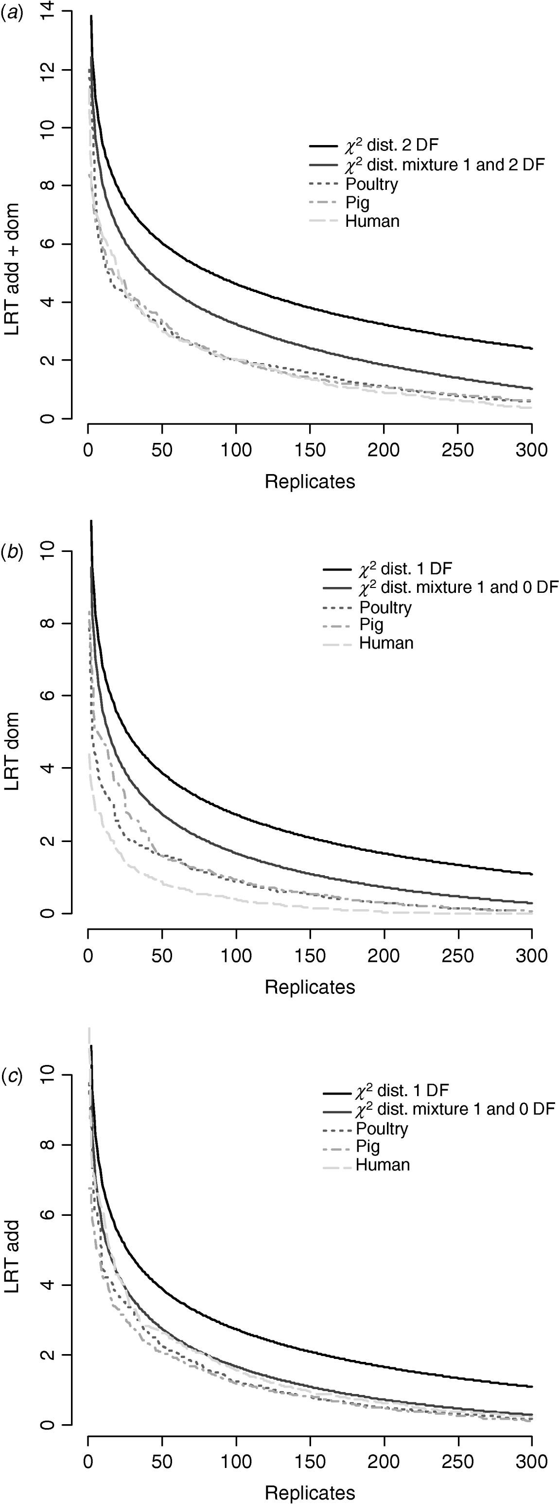
Fig. 6. Distribution of empirical point-wise test statistic in pig, poultry and human pedigrees for (from top to bottom) (a) additive and dominance effects, (b) dominance effects and (c) additive effects compared with χ21 and χ21−0 distributions. The top 300 values of 1000 replicates are displayed.
Figure 7/Table 6 compares distributions of the test statistic under the null hypothesis of no QTL for eight pedigree structures. These vary from human families with three full-sibs to more complex structures such as poultry with 20 full-sibs and 200 half-sibs. It is apparent that the three human pedigrees, i.e. single dam families, have very similar distributions seemingly regardless of the number of full-sibs. Similarly, the three pedigrees with two dam families have similar distributions to each other but clearly different from those of the human or larger livestock families. The pig and poultry distributions are similar to each other although the pig distribution appears slightly more conservative. The χ21−0 distribution appears to be comparable with the pig and poultry distribution, although again as these were chromosome-wise tests that are uncorrected for multiple testing, they cannot be directly compared with nominal values.
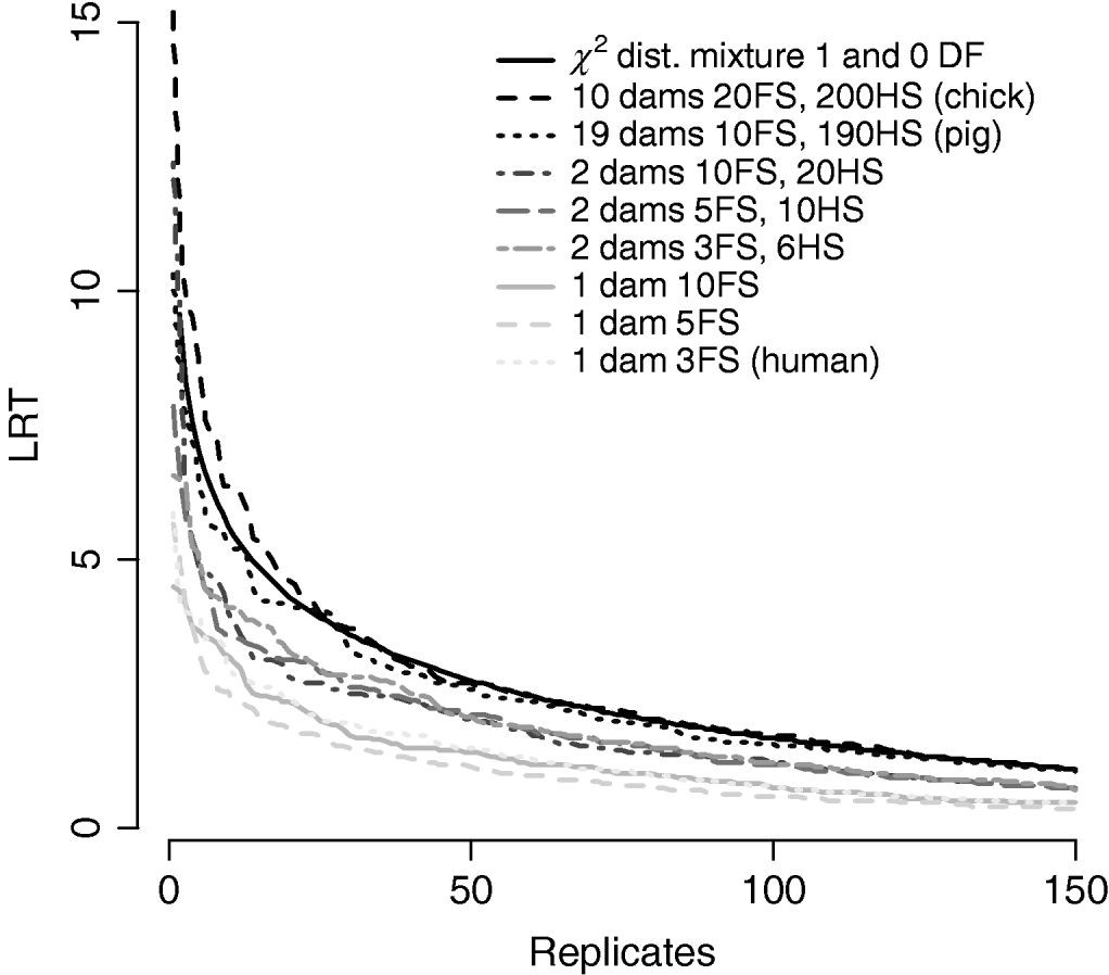
Fig. 7. Comparison of distribution of empirical chromosome-wise test statistic for dominance effects under null hypothesis of no QTL in pedigrees with varying full-sib (FS) and half-sib (HS) structures. χ21−0 is also plotted for comparison. All pedigrees have 1900 total offspring. The top 150 values of 1000 replicates are displayed for clarity.
Table 6. Empirical 5% thresholds for LRT test statistic when testing for dominance and corresponding P value under χ21 distribution. A total of 1000 replicates simulated for chromosome-wise testing under the null scenario of no QTL effects

4. Discussion
This study provides a comprehensive evaluation of the performance of VC analysis over a range of dominant QTL effects. The method was successfully used to estimate and apportion variances due to polygenic, additive, dominant and non-genetic effects. Power >95% was achieved when testing for dominant QTL effects accounting for 7% of the total variance for a simulated poultry population. Power to detect additive QTL was also high (~97% for an additive effect explaining 7% of phenotypic variance. Although the upper range of the simulated QTL effects is high, these values are plausible in terms of the published literature.
Simulation results showed that, unlike the test for additive QTL effects, the empirical distribution of the test statistic when testing for dominant QTL effects did not behave in accordance with existing theoretical expectations. Theoretically, the asymptotic distribution of the LRT is a mixture of χ2 with different degrees of freedom when testing VCs under the null hypothesis that they are zero (Self & Liang, Reference Self and Liang1987; Stram & Lee, Reference Stram and Lee1994). For example, with one extra VC, the null distribution is a mixture of ½ χ0 (i.e. variance is zero) and ½ χ1 (i.e. variance is non-zero). With a model including two VCs, such as additive and dominant QTL effects, the expectation of the distribution would be a mixture of ¼ χ0 (both VCs are zero), ½ χ1 (one is non-zero) and ¼ χ2 (both are non-zero). Visscher (Reference Visscher2006) provides a thorough review.
Problems with incorrect assumptions about the distribution include inflated type II errors leading to reduced power. Extending the linear model to include a dominance component resulted in a conservative test when imposing a χ21 distribution for the LRT statistic. The test remained conservative even when thresholds were halved under the assumption of a mixture of distributions. One explanation might be that additive and dominant QTL effects are not entirely independent. Furthermore, the null distribution for the dominance test varies with family structure, in particular, with the number of dam families per sire. Distributions of the test statistic in Figure 7/Table 6 appear to group by number of dam families, with human-type pedigrees with a single dam per sire most conservative, regardless of family size. The number of full-sibs within dam families did not appear to affect the distribution. It is possible that the lack of half-sib families might result in confounding of additive and dominance effects at the QTL. Theoretically, if both components need to be estimated within dam, lack of information might lead to a higher probability of VCs being zero.
Results showed that power is also affected by population structure. Power to detect dominance at the QTL was similar for pig and poultry populations but much lower for humans.
This was unsurprising as the human population consisted of many small families with low numbers of full-sibs, making it difficult to detect dominance. Increased power might be achieved in human studies from a pedigree with more generations providing information from relationships such as grandparents and cousins, but this needs to be explored further.
It is anticipated that further correction for multiple testing for large linkage groups or genome-wide testing would be necessary. The distribution, however, of H 0 when testing for multiple linked positions is unresolved and authors have used different approximations (Xu & Atchley, Reference Xu and Atchley1995; Pratt et al., Reference Pratt, Daly and Kruglyak2000; Piepho, Reference Piepho2001; Nagamine et al., Reference Nagamine, Visscher and Haley2004). Procedures such as permutation and bootstrapping enable the setting of empirical thresholds and circumvent problems associated with failure of distributional assumptions and independence of multiple tests (Churchill & Doerge, Reference Churchill and Doerge1994; Visscher et al., Reference Visscher, Thompson and Haley1996), although computational complexity can restrict their use within the VC framework.
The method described by Piepho relies on the gradient of change in likelihood. However, this method still assumes that the test statistic for a single test follows a standard χ2 distribution under the null hypothesis and therefore does not address the issue of mixture distributions that is apparent for these types of analyses. It is difficult to ascertain whether the method is appropriate here, when the test statistic follows a mixture of distributions and likelihoods under the null scenario are very flat.
There is strong evidence to suggest that a common environment effect should be routinely evaluated in all VC QTL models as, if unaccounted for, most of the variation due to common environment masquerades as dominance. We have shown that the presence of common environmental effects has little effect on false-negative rates but a potentially huge impact on false-positive rates.
We demonstrated that incorporating a dominance effect in a genome scan has very limited detrimental effect on the power to detect purely additive QTL. Detection of spurious dominance was also rare, suggesting that dominance could be routinely included in genome scans. We have also shown by simulation that, if not fitted in the analysis model, dominance may be detected as spurious additive effects or inflated estimates of additive genetic variance. This suggests that dominant QTL effects can be detected as additive QTL when additive-only models are used; see also Misztal et al. (Reference Misztal, Varona, Culbertson, Bertrand, Mabry, Lawlor, Van Tassell and Gengler1998) and Pante et al. (Reference Pante, Gjerde, McMillan and Misztal2002) for similar effects with polygenic dominance. This has important implications for predicting response to selection as the success of any selection programme is dependent on correctly identifying the mode of inheritance and proportion of variance explained by the QTL. For example, Hayes & Miller (Reference Hayes and Miller2000) have shown that including dominance effects in mate selection can be a powerful tool for exploiting previously untapped genetic variation, whereas Dekkers & Chakraborty (Reference Dekkers and Chakraborty2004) have discussed maximization of crossbred performance by incorporating information from overdominant QTL.
A further confounding factor not studied here might be polygenic dominance. It is, however, unlikely to have affected our results as most of the information for polygenic dominance would have come from the covariance of full-sibs and should have been accounted for by the common environment effect. This might not be the case within other relationships in deeper, more complex, pedigrees, suggesting that the inclusion of a polygenic dominance effect may be valuable when examining such data structures.
5. Conclusions
VC methods were implemented to detect dominant QTL. Type 1 error rates and power were explored using extensive simulations. Results indicate that if the mixture of distributions is taken into account, nominal χ2 thresholds were appropriate when testing for additive QTL but conservative when testing for dominant QTL in all pedigrees and particularly in the case of the populations with sires mated to only one or two dams. Ascertaining the correct null distribution is a difficult issue, but one that merits revisiting. Here, we have shown that although theoretically the tabulated χ2 values are fairly robust, the expected probability of non-zero variances varies with population structure; thus there are instances when greater power is achieved by empirically deriving the correct distribution of the test statistic. Power to detect dominant QTL effects was high in livestock pedigrees with little spurious dominance and could be successfully routinely employed under the proviso that common environment or direct maternal effects are accounted for.
Effects of extra generations or extended pedigrees are yet to be explored but may provide greater power for structures with few dam families. Future aims are to extend the linear model to include other non-additive effects such as epistasis and to simulate behaviour of the test statistic under varying modes of inheritance, size and structure of pedigree.
We thank the reviewers for their helpful comments. We also thank the Biotechnology and Biological Sciences Research Council, the Research Councils UK, Genesis Faraday and Cobb Vantress for funding.


