1. Introduction
Selection of economically important quantitative traits in animals and plants is traditionally based on phenotypic records of an individual and its relatives. High-density panels of single-nucleotide polymorphisms (SNP) have recently been used to map genes of domestic animal species and select desirable livestock (Goddard & Hayes, Reference Goddard and Hayes2009). The genetic merit of an individual can be estimated by genome-wide marker-assisted selection (GWMAS), also known as genomic selection (Meuwissen et al., Reference Meuwissen, Hayes and Goddard2001). Such selection is expected to improve the precision of genetic merit predictions because some markers from a dense SNP panel will be in linkage disequilibrium with quantitative trait loci (QTLs) (Hayes et al., Reference Hayes, Vissher and Goddard2009). Genomic selection will lead to faster genetic gain than that achieved with traditional selection methods based on pedigree and phenotypic data only.
Genome-wide evaluation methods use statistical tools to combine phenotypes with high-density marker data to predict the genetic merit of individuals with complex traits. No agreement exists currently on which genome-wide evaluation method is the most appropriate (Daetwyler et al., Reference Daetwyler, Pong-Wong, Villanueva and Woolliams2010; Hill, Reference Hill2010). Most developments in genome-wide evaluation methods published to date assume that all animals have been genotyped. However, it is rarely the case, and most often non-genotyped close family members exist with phenotypic information (Garrick et al., Reference Garrick, Taylor and Fernando2009). Ignoring this information results in less accurate predictions and possible bias because of selection (VanRaden et al., Reference VanRaden, Van Tassell, Wiggans, Sonstegard, Schnabel, Taylor and Schenkel2009a, Reference VanRaden, Tooker and Coleb). Unbiased predictions are of paramount importance in selection for accurate estimates of the genetic trend and also comparison of animals across generations (Henderson et al., Reference Henderson, Kempthorne, Searle and von Krosigk1959). The acceptance and wide use of genomic predictions will largely depend on correct statistical modelling and ease of breeder application. Therefore, a genetic evaluation method that produces accurate and unbiased predictions is critically important.
Combining pedigree, phenotypic and marker information to calculate genomic predictions is a challenge. The number of genotyped individuals is extremely small compared with the total number of individuals. Some genotyped individuals (as in dairy cattle) do not have a phenotype of their own. Thus, most proposed methods currently are based on multiple-step procedures (VanRaden et al., Reference VanRaden, Van Tassell, Wiggans, Sonstegard, Schnabel, Taylor and Schenkel2009a). First, phenotypic data from relatives are summarized to create pseudodata for genotyped individuals (Garrick et al., Reference Garrick, Taylor and Fernando2009); then in the second step, genomic predictions are computed by a genome-wide method from pseudodata and marker information. For example, in dairy cattle, pseudodata for males are measures of (precorrected) daughter performance called daughter yield deviations (DYD). The use of DYD may involve several problems (VanRaden et al., Reference VanRaden, Van Tassell, Wiggans, Sonstegard, Schnabel, Taylor and Schenkel2009a, Reference VanRaden, Tooker and Coleb): information loss of animals with few progeny, which leads to accuracy loss; heterogeneity caused by different amounts of information in the original dataset; and bias (caused by selection). For other species (e.g. sheep or swine) or traits (e.g. maternal traits), pseudodata are more difficult to estimate or even define. Thus, multiple-step methods of computing genomic predictions are not only complicated but likely suboptimal for GWMAS.
Joint use of pedigree, phenotypic and genomic information should theoretically solve such problems. A single-step method based on a linear mixed model and a pedigree relationship matrix augmented with genomic information has been developed recently (Legarra et al., Reference Legarra, Aguilar and Misztal2009; Aguilar et al., Reference Aguilar, Misztal, Johnson, Legarra, Tsuruta and Lawlor2010; Christensen & Lund, Reference Christensen and Lund2010). This method combines pedigree and all available phenotypes and genotypes, needs no creation of pseudodata, and it has been applied to population sizes in the millions (Aguilar et al., Reference Aguilar, Misztal, Johnson, Legarra, Tsuruta and Lawlor2010). Further, the method is general with straightforward extension to other models or species.
In traditional pedigree-based evaluation, all information about selection decisions is included in phenotypes and the relationship matrix, and no bias exists from the selection (Sorensen & Kennedy, Reference Sorensen and Kennedy1984; Im et al., Reference Im, Fernando and Gianola1989). However, how selection is accounted for in GWMAS procedures is unclear, although this is becoming a serious concern (Aguilar et al., Reference Aguilar, Misztal, Johnson, Legarra, Tsuruta and Lawlor2010; Mäntysaari et al., Reference Mäntysaari, Liu and VanRaden2010; Chen et al., Reference Chen, Misztal, Aguilar, Legarra and Muir2011). Models for GWMAS implicitly assume an unselected genotyped population (Hayes et al., Reference Hayes, Vissher and Goddard2009). However, in practice, genotyped individuals are highly selected, and GWMAS models do not take this selection into account. This is in contrast to classical procedures in which models refer to a base unselected population. Thus, GWMAS models appear to be unable to consider past selection based on pedigree and phenotypes, which might cause bias as well as accuracy loss.
The objective of this study was to investigate how unbiased genetic values can be predicted by GWMAS. The effects of selection and genome-wide evaluation method (single- or multiple-step) on bias and prediction accuracy were examined. The effect of trait heritability was also investigated.
2. Materials and methods
(i) Theory
The single-step genomic prediction approach (Legarra et al., Reference Legarra, Aguilar and Misztal2009; Aguilar et al., Reference Aguilar, Misztal, Johnson, Legarra, Tsuruta and Lawlor2010; Christensen & Lund, Reference Christensen and Lund2010) is based on the model y=Xb+Zu+e, where y is the phenotype vector, X and Z are incidence matrices, b denotes fixed effects, e is the residual and p(u)~N(0, Hσu2) involves the genetic effect for non-genotyped (u1) and genotyped (u2) individuals and the genetic variance σu2. Here H−1 is derived as in Legarra et al., (Reference Legarra, Aguilar and Misztal2009) and Christensen & Lund (Reference Christensen and Lund2010) :
where G is a genomic relationship matrix and ![]() and
and ![]() are the pedigree-based relationship matrix and its inverse partitioned into non-genotyped and genotyped individuals, respectively. Creation of H (and H−1) can be seen as a projection of genetic merit (or marker genotypes) from genotyped to non-genotyped individuals using pedigree relationships (Legarra et al., Reference Legarra, Aguilar and Misztal2009; Christensen & Lund, Reference Christensen and Lund2010).
are the pedigree-based relationship matrix and its inverse partitioned into non-genotyped and genotyped individuals, respectively. Creation of H (and H−1) can be seen as a projection of genetic merit (or marker genotypes) from genotyped to non-genotyped individuals using pedigree relationships (Legarra et al., Reference Legarra, Aguilar and Misztal2009; Christensen & Lund, Reference Christensen and Lund2010).
The pedigree relationship matrix A implies that the mean genetic value of the base population is 0. Also, according to VanRaden (Reference VanRaden2008) and Hayes et al. (Reference Hayes, Vissher and Goddard2009), the genomic relationship matrix G automatically sets the mean genetic value of the genotyped population to 0 if raw means in the genotyped population are used to estimate current allele frequencies. That is not the case if frequencies for the base population are used, but accurate estimates of those frequencies are difficult to obtain.
If selection occurs, the mean genetic value of genotyped individuals (u2) on the scale of the whole population (i.e. relative to the base population) may have a value different from 0, say μ. This would be particularly true if genotyped individuals were elite individuals or in the last generations of selection. Let us assume that μ is a random variable; for instance, in (conceptual) repetitions of the selection process, μ will vary due to drift, in other words, because of finite sampling of replacement animals. Thus, p(μ)~N(0, ασu2); and, p(u2|μ)~N(1μ, Gσu2), where 1 is a vector of ones. Equivalently, p(u2|α)~N(0, (G+11′α)σu2).
As in Legarra et al. (Reference Legarra, Aguilar and Misztal2009), the distribution of genetic values of non-genotyped individuals conditioned on genetic values of genotyped individuals (using multivariate normality) is p(u1|u2)~N(A12 A22−1 u2, (A11)−1 σu2), where (A11)−1=A11−A12 A22−1 A21. Thus, p(u1|α)~N(0, (A11)−1 σu2+A12 A22−1(G+11′α)A22−1 A21σu2) and p(u)~N(0, H†σu2), where H† is equivalent to H with G substituted for G+11′α. The mixed model equations are
where
![{\bf H}^{\dag \minus \setnum{1}} \equals \left[ {\matrix{ {{\bf A}^{\setnum{11}} } \tab {{\bf A}^{\setnum{12}} } \cr {{\bf A}^{\setnum{21}} } \tab {{\bf A}^{\setnum{22}} \plus \lpar {\bf G} \plus {\bf 11 \prime}\alpha \rpar ^{ \minus \setnum{1}} \minus {\bf A}_{\setnum{22}}^{ \minus \setnum{1}} } \cr} } \right].](https://static.cambridge.org/binary/version/id/urn:cambridge.org:id:binary:20160920235920730-0651:S001667231100022X:S001667231100022X_eqn2.gif?pub-status=live)
An equivalent model for unbiased genomic predictions based on a genetic group model (Quaas, Reference Quaas1988) is shown in the appendix.
To determine why μ can be presumed as a random variable and obtain the value of α, traditional best-linear unbiased prediction (BLUP) will be assumed to be unbiased and able to account properly for selection and drift (Sorensen & Kennedy, Reference Sorensen and Kennedy1984). We suggest that the mean value μ of genetic effects of genotyped individuals u2 can be expressed as ![]() , where n is the number of individuals. Since μ is a function of random variables, it is a random variable in itself. The variable μ can be estimated from either pedigree (μp) or single-step (μs) procedures. If genetic prediction based on pedigree (and phenotypic data) is unbiased and accounts for selection and drift, the distribution of μp accounts properly for bias, selection and drift as well. The prior distributions for genetic values of u2 are u2p~N(0, A22σu2) and u2s~N(0, (G+11′α)σu2); thus, the distribution of μ is
, where n is the number of individuals. Since μ is a function of random variables, it is a random variable in itself. The variable μ can be estimated from either pedigree (μp) or single-step (μs) procedures. If genetic prediction based on pedigree (and phenotypic data) is unbiased and accounts for selection and drift, the distribution of μp accounts properly for bias, selection and drift as well. The prior distributions for genetic values of u2 are u2p~N(0, A22σu2) and u2s~N(0, (G+11′α)σu2); thus, the distribution of μ is ![]() and
and
![\eqalign{ \tab \mu _{\rm s} \sim N\left( {{\bf 0}\comma {{\rm 1} \over {n^{\setnum{2}} }}{\bf 1 \prime }\lpar {\bf G}{\rm \plus }{\bf 11 \prime }\alpha \rpar {\bf 1}\sigma _{u}^{\setnum{2}} } \right) \cr \tab \quad \equals N\left( {{\bf 0}\comma {{\rm 1} \over {n^{\setnum{2}} }}{\bf 1 \prime }}\left( {{\bf G \plus }\left[ {\matrix{ \alpha \tab \cdots \tab \alpha \cr \vdots \tab {} \tab \vdots \cr \alpha \tab \cdots \tab \alpha \cr} } \right]} \right){\bf 1}\sigma _{u}^{\setnum{2}} } \right).}](https://static.cambridge.org/binary/version/id/urn:cambridge.org:id:binary:20160920235920730-0651:S001667231100022X:S001667231100022X_eqnU6.gif?pub-status=live)
Since the 1′1 are simply summations,
and

In order to construct a model with features similar to pedigree-based BLUP, we equate the two variances in eqns (3) and (4) and this gives

Thus, α is simply the difference between means for A22 and G. The α accounts for the fact that genotyped animals in u2 are more related through pedigree (in reference to the base population), which is correctly considered in A22. The genomic relationship matrix G does not correctly reflect this fact, especially if current allele frequencies are used, which sets the genomic base as the genotyped individuals (Oliehoek et al., Reference Oliehoek, Winding, van Arendonk and Bijma2006; Van Raden, Reference VanRaden2008). For G to be correct, base allele frequencies would be required. In practice, current allele frequencies are used because base allele frequencies are difficult to estimate. For a population of unrelated individuals where A22=I, α=0.
From Wright's F ST, another interpretation of α is also possible. The F ST can be defined as the mean relationship between gametes in a recent population with respect to an older base population (Cockerham, Reference Cockerham1969, Reference Cockerham1973; Powell et al., Reference Powell, Vissher and Goddard2010). Then A22 involves relationships of genotyped individuals with reference to the base population, and G corresponds to relationships within the current population. Consequently, α is equal to twice F ST; the factor of two is needed because F ST is referred to as co-ancestries, which are half individual additive relationships. The correction suggested by Powell et al. (Reference Powell, Vissher and Goddard2010) is F old=F new+(1−F new) F ST, which is equivalent to ![]() and similar to our suggestion.
and similar to our suggestion.
(ii) Simulations
To evaluate the effectiveness of the proposed approach for genomic prediction, two selection scenarios with different heritabilities were simulated. The simulator QMSim (Sargolzaei & Schenkel, Reference Sargolzaei and Schenkel2009) was used to generate historical (undergoing drift and mutation) and recent (undergoing selection) population structures. In total, 10 chromosomes of equal length (100 cM) were simulated. Biallelic markers (10 000) were distributed at random along the chromosomes with equal frequency in the first generation of the historical population. Potentially, 250 QTLs affect the phenotype; QTLs allele effects were sampled from a Gamma distribution with a shape parameter of 0·4. The mutation rate of the markers (recurrent mutation process) and QTL was assumed to be 2·5×10−5 per locus per generation (Solberg et al., Reference Solberg, Sonesson, Woolliams and Meuwissen2008).
First, a base population of 200 males and 2600 females was generated by mutation and drift over 100 generations (t) in a historical population with an effective population size of 100 (t=1–95) and gradually expanded to 3000 offspring (t=100). Then, 10 generations (t=101–110) of selection for a sex-limited trait with a phenotypic variance of 1 were simulated. Three heritabilities (0·05, 0·30 and 0·50) were used to examine the effect of heritability on genomic predictions. In each generation, 200 males were mated to 2600 females to produce 2600 offspring following random phenotype (PY) or positive assortative (matings among best males and females based on estimated breeding values (EBVs); PEBV) designs. For the next generation, 80 males and 520 females were selected based on PY or PEBV. For PEBV, EBVs were computed in each generation with data accumulated so far by a BLUP procedure that includes phenotypes and pedigree, which mimics recent selection procedures for livestock populations. At the end of each simulation, true genetic values (TBVs) and pedigree information were available for all ten generations (28 800 individuals in pedigree), phenotypes were available for all generations except for the last one (13 100 records). All males (840 sires of females with records) were genotyped as well as 260 individuals in generation 110, which were potential candidates for selection. No fixed effects were simulated. For each scenario, 20 replicates were run.
(iii) Prediction methods
The 260 genotyped selection candidates in the last generation were evaluated using genomic information. Genetic merit of the selection candidates was estimated using five methods based on BLUP. The first method was a mixed model based on the pedigree relationship matrix and phenotypes (BLUPPED). The second method was a two-step procedure, in which DYD were computed using a regular method based on pedigree and phenotypes and then used for genomic prediction (BLUPDYD). For BLUPDYD, 840 males were included with DYD information from 14 (±10) daughters on average. The DYD were weighted by their accuracy. For the third method, the full dataset (pedigree, phenotypes and genotypes) was directly used in a single-step procedure that used G (BLUP1STEP). The fourth method (BLUPα) is also a single-step procedure with the correction of genetic differences among genotyped and non-genotyped individuals simply by using H†−1, which uses G†=G+11′α instead of G. The correction of G proposed by Powell et al. (Reference Powell, Vissher and Goddard2010) was also implemented using ![]() and tested in a single-step procedure (
and tested in a single-step procedure (![]() ).
).
All single-step methods (BLUP1STEP, BLUPα and ![]() ) and BLUPDYD used
) and BLUPDYD used ![]() , where z i was coded as −p i or 1−p i for the first or second allele, respectively, and p i is the allele frequency of the second allele (VanRaden, Reference VanRaden2008) computed as raw mean from all available genotypes.
, where z i was coded as −p i or 1−p i for the first or second allele, respectively, and p i is the allele frequency of the second allele (VanRaden, Reference VanRaden2008) computed as raw mean from all available genotypes.
Prediction quality was checked for all 260 selection candidates (validation data). Bias was measured as the difference between predicted and simulated breeding values of the candidates. Regression of TBV on EBV was used as a measure of the inflation of the prediction method, where a regression coefficient of one denotes no inflation. Accuracy of evaluation methods was computed as the square of the correlation between TBV and EBV. In addition, prediction error variance (PEV), which is a measure of candidate prediction error, and mean-squared error (MSE), which is a measure of overall fit of the model to the data, were computed. Results were the mean of the 20 replicates of each scenario.
3. Results
(i) Correction factor
Table 1 shows mean α for the three heritabilities under PY or PEBV. The variance α is higher for selection predominantly on relatives (e.g. low heritability traits under PEBV). Bias, inflation and accuracy of predictions as a function of α for a given replicate are presented in Fig. 1. In the example, the theoretical value of α according to eqn (5) was 0·07, which was α where bias was close to zero but not the smallest. Optimally, high accuracy (R 2) and low inflation (b) should be balanced to avoid large bias increases.
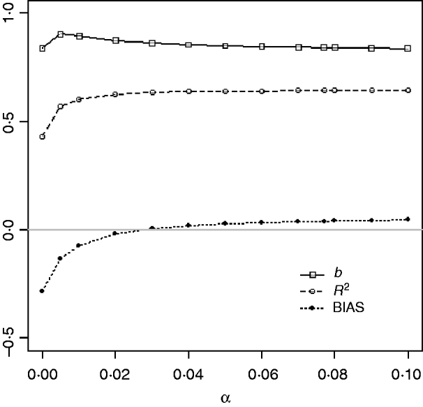
Fig. 1. Bias (dotted curve with solid circles), coefficient of regression of true on EBV (b; solid curve with squares), and squared correlation between true and EBVs (R 2; dashed curve with circles) as functions of the correction factor α (difference between pedigree-based and genome-based relationships for genotyped animals) for a given replicate with heritability of 0·30 under assortative mating selection based on EBV.
Table 1. Mean α for different heritabilities under PY or PEBV selection
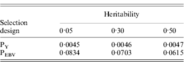
α is the difference between pedigree-based and genome-based relationships for genotyped animals; selection was based either on random phenotype (PY) or assortative mating using EBV (PEBV).
(ii) Bias
Table 2 shows TBV and EBV means from the five prediction methods under PY or PEBV for the selection candidates in the last generation. Mean TBV of the last generation was 3·2–5·4 times larger for PEBV than for PY. As expected, even with selection and different heritabilities, BLUPPED predicted mean TBV correctly. The BLUPDYD and BLUP1STEP methods underestimated mean TBV in the last generation, but BLUPα and ![]() were unbiased.
were unbiased.
Table 2. Means (SDs) of breeding values from different heritabilities and prediction methods for selection candidates under PY and PEBV
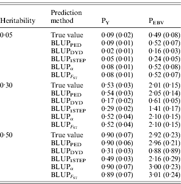
Prediction methods were based on BLUP: a mixed model based on the pedigree relationship matrix and phenotypes (BLUPPED), a two-step procedure in which DYD were computed from a regular method based on pedigree and phenotypes and then used for genomic prediction (BLUPDYD), a single-step procedure that used the genomic relationship matrix and the full dataset of pedigree, phenotypes and genotypes (BLUP1STEP), a single-step procedure with genetic differences among genotyped and non-genotyped individuals corrected by considering the difference between pedigree-based and genome-based relationships for genotyped animals (BLUPα) and a single-step procedure that corrected the genomic relationship matrix as proposed by Powell et al. (Reference Powell, Vissher and Goddard2010) (![]() ). Selection was based either on random phenotype (PY) or assortative mating using EBV (PEBV).
). Selection was based either on random phenotype (PY) or assortative mating using EBV (PEBV).
(iii) Inflation
The degree of inflation from the prediction methods is indicated by the coefficient of regression of TBV on EBV (Table 3). The optimal prediction method of genetic merit of young individuals would have a regression coefficient close to 1. For each scenario, the differences between the methods were small, and the approaches achieved very similar inflation. A strong selection, under PEBV, increased inflation with values lower than 1. According to Kennedy et al. (Reference Kennedy, Schaeffer and Sorensen1988) relationship matrix accounts for selection, drift and non-random mating, but it does not account for a wrong definition of the base population or a finite number of loci. Potentially 250 QTLs affected the phenotype, and so this discards the second reason. Ideally, the base population should be infinite; this is indeed not the case, and thus the first assumption is violated. Consider animals 1 and 2 (e.g. father and son). If they are related, the distribution of the genetic value of 2 can expressed as conditioned on the genetic value of 1. Thus, knowledge of the EBV of 1 would decrease uncertainty (variance) of the EBV of 2. However, if this relationship is unknown, the conditional distribution cannot be written. Thus, not knowing relationships will increase the variance of EBVs and cause inflation; this has not been verified.
Table 3. Coefficients (SDs) for regression of true on EBV for different heritabilities and prediction methods under PY and PEBV
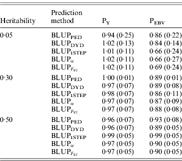
Prediction methods were based on BLUP: a mixed model based on the pedigree relationship matrix and phenotypes (BLUPPED), a two-step procedure in which DYD were computed from a regular method based on pedigree and phenotypes and then used for genomic prediction (BLUPDYD), a single-step procedure that used the genomic relationship matrix and the full dataset of pedigree, phenotypes and genotypes (BLUP1STEP), a single-step procedure with genetic differences among genotyped and non-genotyped individuals corrected by considering the difference between pedigree-based and genome-based relationships for genotyped animals (BLUPα), and a single-step procedure that corrected the genomic relationship matrix as proposed by Powell et al. (Reference Powell, Vissher and Goddard2010) (![]() ). Selection was based either on random phenotype (PY) or assortative mating using EBV (PEBV).
). Selection was based either on random phenotype (PY) or assortative mating using EBV (PEBV).
(iv) Accuracy
Squared correlations between TBV and EBV (i.e. reliability) by heritability and prediction method are shown in Table 4. Squared correlations are presented in Fig. 2 for all replicates using a heritability of 0·30 under PEBV. Compared with BLUPPED, all genomic prediction methods increased accuracy by about 37 percentage units and 22 percentage units under assortative mating based on EBV and mass selection, respectively.
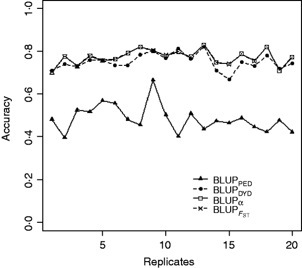
Fig. 2. Accuracy (squared correlations between true and EBV) of BLUP methods for estimating breeding value of selection candidates across 20 replicates with heritability of 0·30 under assortative mating selection based on EBV. Prediction methods were a mixed model based on the pedigree relationship matrix and phenotypes (BLUPPED; solid line with triangles), a two-step procedure in which DYD were computed from a regular method based on pedigree and phenotypes and then used for genomic prediction (BLUPDYD; dashed line with solid circles), a single-step procedure with genetic differences among genotyped and non-genotyped individuals corrected by considering the difference between pedigree-based and genome-based relationships for genotyped animals (BLUPα; solid line with squares) and a single-step procedure that corrected the genomic relationship matrix as proposed by Powell et al. (Reference Powell, Vissher and Goddard2010) (![]() ) (dashed line with x markers).
) (dashed line with x markers).
Table 4. Squared correlations between true and EBVs (SDs) for different heritabilities and prediction methods under PY and PEBV
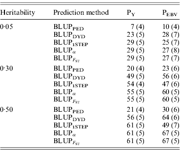
Squared correlations between true and EBVs were expressed as percentages. Prediction methods were based on BLUP: a mixed model based on the pedigree relationship matrix and phenotypes (BLUPPED), a two-step procedure in which DYD were computed from a regular method based on pedigree and phenotypes and then used for genomic prediction (BLUPDYD), a single-step procedure that used the genomic relationship matrix and the full dataset of pedigree, phenotypes and genotypes (BLUP1STEP), a single-step procedure with genetic differences among genotyped and non-genotyped individuals corrected by considering the difference between pedigree-based and genome-based relationships for genotyped animals (BLUPα) and a single-step procedure that corrected the genomic relationship matrix as proposed by Powell et al. (Reference Powell, Vissher and Goddard2010) (![]() ). Selection was based either on random phenotype (PY) or assortative mating using EBV (PEBV).
). Selection was based either on random phenotype (PY) or assortative mating using EBV (PEBV).
With low heritability under PEBV, accuracy from BLUPα and ![]() was as good as from BLUPDYD (Table 4). When these accuracies are comparable, the single-step procedures with correction (BLUPα and
was as good as from BLUPDYD (Table 4). When these accuracies are comparable, the single-step procedures with correction (BLUPα and ![]() ) have an advantage over BLUPDYD because they provide a unified framework that eliminates all the assumptions applied in multiple-step methods. With medium or high heritabilities under PEBV, BLUPα and
) have an advantage over BLUPDYD because they provide a unified framework that eliminates all the assumptions applied in multiple-step methods. With medium or high heritabilities under PEBV, BLUPα and ![]() have the highest accuracies (Table 4; Fig. 2). The lower accuracy of BLUPDYD compared with BLUPα and
have the highest accuracies (Table 4; Fig. 2). The lower accuracy of BLUPDYD compared with BLUPα and ![]() results from ignoring parent average in BLUPDYD. Including parent average in predictions increases the accuracy in multiple-step methods, but it is complicated (VanRaden et al., Reference VanRaden, Van Tassell, Wiggans, Sonstegard, Schnabel, Taylor and Schenkel2009a). Parent averages are automatically included in genomic predictions with single-step methods.
results from ignoring parent average in BLUPDYD. Including parent average in predictions increases the accuracy in multiple-step methods, but it is complicated (VanRaden et al., Reference VanRaden, Van Tassell, Wiggans, Sonstegard, Schnabel, Taylor and Schenkel2009a). Parent averages are automatically included in genomic predictions with single-step methods.
(v) Other comparison measures
In addition to assessing the quality of genetic evaluations through bias and accuracy from the difference and correlation between TBV and EBV, PEV and MSE were also considered (Table 5). All genomic methods had the lowest PEV under PY for all heritabilities. Under PEBV, PEV also were lowest for genomic methods except with low heritability. Compared with MSE for BLUPDYD predictions, MSE for BLUPα were 18–66% lower under PY and 60–96% lower under PEBV, with differences increasing with heritability under both selection designs. The greatly decreased MSE for all scenarios indicated that the multiple-step BLUPDYD was less accurate. Considering the potential genetic gain from selection, BLUPα and ![]() were the most advantageous prediction methods.
were the most advantageous prediction methods.
Table 5. PEVs (SDs) and MES (SDs) for different heritabilities and prediction methods under PY and PEBV
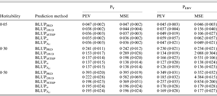
PEV and MSE are shown. Prediction methods were based on BLUP: a mixed model based on the pedigree relationship matrix and phenotypes (BLUPPED), a two-step procedure in which DYD were computed from a regular method based on pedigree and phenotypes and then used for genomic prediction (BLUPDYD), a single-step procedure that used the genomic relationship matrix and the full dataset of pedigree, phenotypes and genotypes (BLUP1STEP), a single-step procedure with genetic differences among genotyped and non-genotyped individuals corrected by considering the difference between pedigree-based and genome-based relationships for genotyped animals (BLUPα), and a single-step procedure that corrected the genomic relationship matrix as proposed by Powell et al. (Reference Powell, Vissher and Goddard2010) (![]() ). Selection was based either on random phenotype (PY) or assortative mating using EBV (PEBV).
). Selection was based either on random phenotype (PY) or assortative mating using EBV (PEBV).
4. Discussion
Comparison of the four genomic prediction methods at various heritabilities under two selection intensities demonstrated that a single-step method with correction (either BLUPα or ![]() ) was a preferred method of accounting for bias in genomic predictions. Furthermore, two possible G for prediction of genetic merit were tested. Genomic preselection of animals often is included in dairy cattle breeding programmes now. Thus, bias becomes an important concern with the multiple-step method, because computation of DYD assumes random selection of the Mendelian sampling, which is clearly violated (Patry & Ducrocq, Reference Patry and Ducrocq2011). Because single-step methods do not create pseudodata and are unbiased, they may be an attractive genomic evaluation method.
) was a preferred method of accounting for bias in genomic predictions. Furthermore, two possible G for prediction of genetic merit were tested. Genomic preselection of animals often is included in dairy cattle breeding programmes now. Thus, bias becomes an important concern with the multiple-step method, because computation of DYD assumes random selection of the Mendelian sampling, which is clearly violated (Patry & Ducrocq, Reference Patry and Ducrocq2011). Because single-step methods do not create pseudodata and are unbiased, they may be an attractive genomic evaluation method.
Bias differences among the methods may be explained by how the different methods account for genotypes of highly selected individuals (i.e. males). Classical theory for modelling covariance among individuals assumes no selection. Thus, covariances among TBVs of selected individuals are no longer described well by any (genomic or pedigree-based) relationship matrix, unless all records used in the selection are accounted for (as in BLUPPED) (Sorensen & Kennedy, Reference Sorensen and Kennedy1984; Kennedy et al., Reference Kennedy, Schaeffer and Sorensen1988). Although all records are used in BLUP1STEP, only genotyped (and mostly selected) individuals are included in G. Since genetic values of non-genotyped animals are, a priori, conditioned on genetic values of genotyped animals (Legarra et al., Reference Legarra, Aguilar and Misztal2009), bias is alleviated but not fully corrected. In a single-step method with correction, such as BLUPα, bias is eliminated by referencing genomic and pedigree-based relationship matrices to the base population. With correction, BLUPα (or ![]() ) is the most accurate for GWMAS.
) is the most accurate for GWMAS.
A pertinent question is which evaluation criterion should be used to maximize genetic gain in selection schemes. According to classical selection theory, best prediction is ideal for selection (Henderson, Reference Henderson1973; Fernando & Gianola, Reference Fernando and Gianola1986). The best predictor minimizes MSE, and is unbiased and not inflated (b=1) by construction (Henderson, Reference Henderson1973). If we were using the best predictor, accuracy, PEV or MSE should provide the same ranking of methods. The best predictor requires knowing the true model generating the data. This is not the case here because true QTLs were not included in the model for genetic evaluation. Instead, we used a linear model assuming multivariate normality.
In practice, the relevance of the criterion used depends on the selection schemes. If the parents of the next generation come from (and only from) genotyped selection candidates, then accuracy is the criterion to maximize, because selection candidates share a common mean (i.e. they belonged to the same generation) and thus bias is not a concern.
If for different candidates there are different amounts of information (e.g. comparing progeny-tested males vs. newborn animals), PEV or MSE have to be considered. For example, in the presence of bias, genetic gain is over (or under) estimated. Thus, newborns are thought to be better than what they are. In this case, MSE is possibly the criterion of choice, because it also includes bias. For instance, Roehe & Kennedy (Reference Roehe and Kennedy1993), who showed that a wrong model resulted in an artificial overestimation of genetic trend, which raised the estimated merit of young selection candidates. Similarly, inflation (b<1, which is included in PEV or MSE but not in accuracy) results in exaggeration (both over and under) of estimated genetic merit of newborns with respect to progeny-tested animals.
However, accuracy is currently used to assess genomic prediction methods in cross-validation studies (e.g. VanRaden et al., Reference VanRaden, Van Tassell, Wiggans, Sonstegard, Schnabel, Taylor and Schenkel2009a), although bias is becoming an increasing concern (e.g. Luan et al., Reference Luan, Woolliams, Lien, Kent, Svendsen and Meuwissen2009; VanRaden et al., Reference VanRaden, Tooker and Cole2009b; Mäntysaari et al., Reference Mäntysaari, Liu and VanRaden2010). Consideration of bias, accuracy and inflation, possibly through MSE, is strongly recommended for the comparison of future genomic selection strategies.
5. Conclusion
Overall, a single-step genomic prediction method with corrected G (BLUPα or ![]() ) was unbiased, similarly inflated and more accurate than other procedures even in the presence of selection. The corrected G is an appropriate methodological solution that takes into account the effect of non-random genotyping (due to strong selection) on prediction. The results clearly showed that a single-step genomic prediction approach is promising for animal/plant breeding.
) was unbiased, similarly inflated and more accurate than other procedures even in the presence of selection. The corrected G is an appropriate methodological solution that takes into account the effect of non-random genotyping (due to strong selection) on prediction. The results clearly showed that a single-step genomic prediction approach is promising for animal/plant breeding.
We are grateful to Paul VanRaden, Daniel Gianola, Daniel Sorensen, Shogo Tsuruta and Ching-Yi Chen for their helpful and constructive comments. This work was partly financed by Holstein Association USA, Smithfield Premium Genetics, the National Beef Cattle Evaluation Consortium and AFRI grants 2009-65205-05665 and 2010-65205-20366 from the USDA NIFA Animal Genome Program (ZV, IA, IM) as well as Apisgene and ANR projects AMASGEN and SheepSNPQTL and POCTEFA project Genomia (AL). The project also was partly supported by the Genopole Toulouse Midi-Pyrénées bioinformatics platform.
Appendix
Genetic group model for unbiased genomic predictions
From the model of unbiased genomic predictions presented in section (i), we have that
p(u2|μ)~N(1μ, Gσu2),
and p(u|μ)~N(Qμ, Hσu2), where H is according to eqn (1) and Q is ![]() .
.
The setting is like a genetic group model (Quaas, Reference Quaas1988) and equivalent mixed-model equations, which yields the same solutions for b and u, is derived as in Quaas (Reference Quaas1988) as
![\left[ {\matrix{ {{\bf X \prime X}} \tab {{\bf X \prime Z}} \tab {\bf 0} \cr {{\bf Z \prime X}} \tab {{\bf Z \prime Z} \plus {\bf H}^{ \minus \setnum{1}} \lambda } \tab { \minus {\bf H}^{ \minus \setnum{1}} {\bf Q}\lambda } \cr {\bf 0} \tab { \minus {\bf Q \prime H}^{ \minus \setnum{1}} \lambda } \tab {{\bf Q \prime H}^{ \minus \setnum{1}} {\bf Q}\lambda \plus \alpha ^{ \minus \setnum{1}} \lambda } \cr} } \right]\left[ {\matrix{ {\bf b} \cr {\bf u} \cr \mu \cr} } \right] \equals \left[ {\matrix{ {{\bf X \prime y}} \cr {{\bf Z \prime y}} \cr 0 \cr} } \right].](https://static.cambridge.org/binary/version/id/urn:cambridge.org:id:binary:20160920235920730-0651:S001667231100022X:S001667231100022X_eqnU40.gif?pub-status=live)
The above expression is simplified by computing the product Q′H−1 as
![\openup16pt {\eqalign{ \minus {\bf Q \prime H}^{ \minus \setnum{1}} \tab \equals \minus \left[ {\matrix{ {{\bf 1 \prime A}_{\setnum{22}}^{ \minus \setnum{1}} {\bf A}_{\setnum{21}} } \tab {\bf 1} \cr} } \right]\left[ {\matrix{ {{\bf A}^{\setnum{11}} } \tab {{\bf A}^{\setnum{12}} } \cr {{\bf A}^{\setnum{21}} } \tab {{\bf A}^{\setnum{22}} \plus {\bf G}^{ \minus \setnum{1}} \minus {\bf A}_{\setnum{22}}^{ \minus \setnum{1}} } } } \right]\cr \tab \equals \left[ {\matrix{ { \minus {\bf 1 \prime A}_{\setnum{22}}^{ \minus \setnum{1}} {\bf A}_{\setnum{21}} {\bf A}^{\setnum{11}} \minus {\bf 1A}^{\setnum{21}} } \quad{ \minus {\bf 1A}_{\setnum{22}}^{ \minus \setnum{1}} {\bf A}_{\setnum{21}} {\bf A}^{\setnum{12}} \minus } \cr} {\bf 1}\left( {{\bf A}^{\setnum{22}} \plus {\bf G}^{ \minus \setnum{1}} \minus {\bf A}_{\setnum{22}}^{ \minus \setnum{1}} } \right)} \right] \cr \tab \equals \left[ {\matrix{ { \minus {\bf 1 \prime A}_{\setnum{22}}^{ \minus \setnum{1}} {\bf A}_{\setnum{21}} {\bf A}^{\setnum{11}} \minus {\bf 1A}^{\setnum{21}} } \quad{ \minus {\bf 1}\left( {{\bf A}_{\setnum{22}}^{ \minus \setnum{1}} {\bf A}_{\setnum{21}} {\bf A}^{\setnum{12}} \plus {\bf A}^{\setnum{22}} \minus {\bf A}_{\setnum{22}}^{ \minus \setnum{1}} } \right) \minus {\bf 1G}^{ \minus \setnum{1}} } \cr} } \right]. \cr}](https://static.cambridge.org/binary/version/id/urn:cambridge.org:id:binary:20160920235920730-0651:S001667231100022X:S001667231100022X_eqnU41.gif?pub-status=live)
Note that ![]() and
and ![]() . We can see that
. We can see that ![]() and the product
and the product ![]() , which is simply the sum of its elements.
, which is simply the sum of its elements.
Thus, the mixed-model equations can be expressed as
![\left[ {\matrix{ {{\bf X \prime X}} \tab {{\bf X \prime Z}} \cr {{\bf Z \prime X}} \tab {{\bf Z \prime Z} \plus {\bf H}^{\ast \minus \setnum{1}} \lambda } \cr} } \right]\left[ {\matrix{ {\bf b} \cr {\bf \theta } \cr} } \right] \equals \left[ {\matrix{ {{\bf X \prime y}} \cr {{\bf Z \prime y}} \cr} } \right]\comma](https://static.cambridge.org/binary/version/id/urn:cambridge.org:id:binary:20160920235920730-0651:S001667231100022X:S001667231100022X_eqn6.gif?pub-status=live)
with Z′Z appropriately expanded with zeros, ![]() and setting H*−1
as
and setting H*−1
as
![\eqalign{ {\bf H}^{\ast \minus \setnum{1}} \equals \tab \left[ {\matrix{ {{\bf {H}}^{\setnum{11}}} \tab {{\bf { H}}^{\setnum{12}} } \tab {\bf 0} \cr {{\bf {H}}^{\setnum{21}} } \tab {{\bf {H}}^{\setnum{22}} } \tab { \minus {\bf G}^{ \minus \setnum{1}} {\bf 1}} \cr {\bf 0} \tab { \minus {\bf 1 \prime G}^{ \minus \setnum{1}} } \tab {{\bf 1 \prime G}^{ \minus \setnum{1}} {\bf 1} \plus \alpha ^{ \minus \setnum{1}} } \cr} } \right] \cr \tab \equals \left[ {\matrix{ {{\bf A}^{\setnum{11}} } \tab {{\bf A}^{\setnum{12}} } \tab {\bf 0} \cr {{\bf A}^{\setnum{21}} } \tab {{\bf A}^{\setnum{22}} \plus {\bf G}^{ \minus \setnum{1}} \minus {\bf A}_{\setnum{22}}^{ \minus \setnum{1}} } \tab { \minus {\bf G}^{ \minus \setnum{1}} {\bf 1}} \cr {\bf 0} \tab { \minus {\bf 1 \prime G}^{ \minus \setnum{1}} } \tab {{\bf 1 \prime G}^{ \minus \setnum{1}} {\bf 1} \plus \alpha ^{ \minus \setnum{1}} } \cr} } \right].}](https://static.cambridge.org/binary/version/id/urn:cambridge.org:id:binary:20160920235920730-0651:S001667231100022X:S001667231100022X_eqnU47.gif?pub-status=live)
Absorption of μ in (6) gives mixed-model equations with H†−1 (eqn (2)) using expression (2) in Henderson & Searle (Reference Henderson and Searle1981) . Computing H*−1 is similar to the creation of A−1 with genetic groups as reported by Quaas (Reference Quaas1988) .
The expression (6) is of interest because there is an explicit estimate of μ. In addition, mixed-model equations in (6) have a straightforward interpretation. The genetic value of a genotyped individual is conditional on its mean μ and relatives through genomic relationships. The genetic value of a non-genotyped individual is conditional on its relatives through pedigree relationships, including relatives with genotypes.


