


Impact Statement
Fish collective behaviour is an open area of research that continues to attract the interest of a broad scientific community and the curiosity of the general public. How and why do fish align their bodies, synchronize their motion and swim close to each other? And how do they choose one pattern over another? In search for some answers, we establish an experimentally-validated mathematical model for the collective behaviour of zebrafish, a popular species in laboratory research. The model accounts for social and hydrodynamic interactions between animals, and it incorporates key features of the burst-and-coast swimming style of zebrafish. In agreement with experimental observations, the model predicts a strong preference of zebrafish to swim in-line, with one fish leading the other. We mathematically demonstrate that the emergence of this collective pattern is related to its local stability, such that zebrafish interactions will dynamically compensate for any small perturbation to in-line swimming. Interestingly, the stability of in-line swimming is modulated by the distance between the animals, owing to short-range hydrodynamic repulsion. Just as the proposed model is expected to find application in preclinical research on zebrafish, the presented analytical tools create an important connection between stability and collective behaviour.
1. Introduction
The majority of fish species live part of their lives in a group; this affords several advantages, which include enhanced abilities to escape from predators, search for food and find correct migratory routes (Reference LarssonLarsson, 2012). Common to life in a group is swimming together in a school, where fish synchronize their motion in a crystallized formation of tightly-packed individuals (Reference Miller and GerlaiMiller & Gerlai, 2011). The mechanisms underlying the formation of these schooling patterns and their potential hydrodynamic implications have long been the subject of intense debate, which is yet to be resolved (Reference Ashraf, Bradshaw, Ha, Halloy, Godoy-Diana and ThiriaAshraf et al., 2017; Reference Partridge and PitcherPartridge & Pitcher, 1979; Reference WeihsWeihs, 1973).
While experimental research is the cornerstone against which new hypotheses must be tested, mathematical modelling offers a promising approach for detailing the inner workings of collective behaviour. Since the seminal work of Reference AokiAoki (Reference Aoki1982), a number of modelling approaches have been proposed to study collective behaviour (Reference Vicsek and ZafeirisVicsek & Zafeiris, 2012). Reaching beyond agent-based models implementing behavioural rules in discrete time, several authors have proposed modelling approaches based on stochastic differential equations, such as Reference Butail, Mwaffo and PorfiriButail et al. (Reference Butail, Mwaffo and Porfiri2016), Reference Calovi, Lopez, Ngo, Sire, Chaté and TheraulazCalovi et al. (Reference Calovi, Lopez, Ngo, Sire, Chaté and Theraulaz2014, Reference Calovi, Lopez, Schuhmacher, Chaté, Sire and Theraulaz2015) and Reference Zienkiewicz, Barton, Porfiri and Di BernardoZienkiewicz et al. (Reference Zienkiewicz, Barton, Porfiri and Di Bernardo2015a,Reference Zienkiewicz, Barton, Porfiri and Di Bernardob).
Particularly promising is the recent model by Reference Filella, Nadal, Sire, Kanso and EloyFilella et al. (Reference Filella, Nadal, Sire, Kanso and Eloy2018), which considers, for the first time, the presence of hydrodynamic interactions between swimming fish. These interactions are modelled by associating each fish with a vortex dipole, which encapsulates both self-propulsion and the velocity field generated by a swimming fish. The velocity field generated by one fish induces advection and rotation on other animals in the vicinity, and vice versa, thereby providing a mechanism for bidirectional hydrodynamic interactions between fish. While paving the way toward the mathematical integration of social and hydrodynamic interactions, their study was not grounded in experimental observations and all of the claims were based on numerical simulations.
Here, we seek to address these limitations by tailoring the model of Reference Filella, Nadal, Sire, Kanso and EloyFilella et al. (Reference Filella, Nadal, Sire, Kanso and Eloy2018) to real data on pairs of zebrafish, a species of choice in the study of collective behaviour in laboratory settings (Reference Kalueff, Gebhardt, Stewart, Cachat, Brimmer and ChawlaKalueff et al., 2013; Reference Orger and de PolaviejaOrger & de Polavieja, 2017). To achieve this goal, we include realistic turn rate dynamics that capture the burst-and-coast swimming style of zebrafish (Reference Kalueff, Gebhardt, Stewart, Cachat, Brimmer and ChawlaKalueff et al., 2013). We calibrate the model on real data from Reference Zienkiewicz, Barton, Porfiri and Di BernardoZienkiewicz et al. (Reference Zienkiewicz, Barton, Porfiri and Di Bernardo2015a) and demonstrate its predictive power on multiple measures of collective behaviour. Going beyond numerical simulations, we offer analytical insight into the model by elucidating the stability of in-line swimming. This swimming pattern has been experimentally and numerically studied in the technical literature on collective behaviour with multisensory cues, but its stability has never been analytically investigated (Reference De Bie, Manes and KempDe Bie et al., 2020; Reference Kato, Nakagawa, Ohkawa, Muramoto, Oyama, Watanabe and SugitaniKato et al., 2004; Reference Laan, Gil de Sagredo and de PolaviejaLaan et al., 2017; Reference Perna, Grégoire and MannPerna et al., 2014; Reference Saadat, Berlinger, Sheshmani, Nagpal, Lauder and Haj-HaririSadaat et al., 2021).
The rest of the paper is organized as follows: § 2 introduces the modelling framework; § 3 offers analytical insight into the stability of schooling patterns; § 4 discusses calibration of model parameters on experimental results; § 5 presents and discusses the results; and § 6 summarizes the main findings of the work and identifies avenues for future research.
2. Modelling Collective Behaviour of a Zebrafish Pair
We model zebrafish as self-propelled bodies swimming in an unbounded two-dimensional plane. At time  $t$, fish
  $f$
$f$  $(f\in \{1,2\})$ is identified by the position of its centroid
  $\boldsymbol {r}_f(t)$ and swimming direction
  $\hat{\boldsymbol{v}}_f(t)$ with respect to a global reference frame (Figure 1a). Working with a Cartesian coordinate system with unit vectors
  $\hat {\boldsymbol{i}}$ and
  $\hat {\boldsymbol{j}}$ for
  $x$ and
  $y$, respectively, we write
  $\boldsymbol {r}_f(t)=x_f(t)\hat {\boldsymbol{i}}+y_f(t)\hat {\boldsymbol{j}}$ and
  $\hat {\boldsymbol{v}}_f(t)=\cos \theta _f(t)\hat {\boldsymbol{i}}+\sin \theta _f(t)\hat {\boldsymbol{j}}$ (Figure 1a).

Figure 1. Schematic of an interacting zebrafish pair: (a) generic configuration with streamlines overlaid and key variables of fish 1 identified; and (b) in-line schooling pattern, where  $\theta _c$ is the common orientation of the fish and
  $d$ is their inter-individual distance.
Toward the analytical treatment of the problem, we hypothesize that each fish has a constant self-propulsion speed  $v_f$. When swimming in a background flow, the velocity of the animal in the global reference frame is the superposition of self-propulsion and advection. In particular, swimming in a pair causes the speed of fish
  $f$ to dynamically change with respect to the fixed coordinate system owing to the flow created by the other individual in the pair. Specifically, the velocity of the focal fish
  $f$ is given by (Reference Filella, Nadal, Sire, Kanso and EloyFilella et al., 2018)
 \begin{equation} \dot{\boldsymbol{r}}_{f}(t) = v_{f}\hat{\boldsymbol{v}}_{f}(t) + \boldsymbol{U}_f(\boldsymbol{r}_f(t)),\end{equation}
where a superimposed dot means a time derivative and  $\boldsymbol {U}_f(\boldsymbol {r}_f(t))$ is the advection velocity experienced by fish
  $f$ at time
  $t$ owing to the presence of the other fish in the pair.
As a first approximation to the fluid flow generated by the other fish in the pair, we employ the potential flow framework developed by Reference Filella, Nadal, Sire, Kanso and EloyFilella et al. (Reference Filella, Nadal, Sire, Kanso and Eloy2018), Reference Gazzola, Tchieu, Alexeev, de Brauer and KoumoutsakosGazzola et al. (Reference Gazzola, Tchieu, Alexeev, de Brauer and Koumoutsakos2016), Reference Kanso and TsangKanso & Tsang (Reference Kanso and Tsang2015) and Reference Tchieu, Kanso and NewtonTchieu et al. (Reference Tchieu, Kanso and Newton2012), wherein vorticity shedding owing to swimming is neglected and the fluid is modelled as incompressible, inviscid and irrotational. From an application perspective, the most restrictive of these assumptions are those of irrotationality and no vorticity shedding. Irrotationality will be violated in any sort of shear flow, which includes flow near solid boundaries, thereby challenging the use of the model to examine wall-hugging behaviours that could be associated with stress (Reference Kalueff, Gebhardt, Stewart, Cachat, Brimmer and ChawlaKalueff et al., 2013). Furthermore, neglecting vorticity shedding precludes the possibility to examine hydrodynamic interactions when the fish are in close proximity, interacting with each other's wake (Reference WeihsWeihs, 1973).
Following the finite-dipole paradigm, originally proposed by Reference Tchieu, Kanso and NewtonTchieu et al. (Reference Tchieu, Kanso and Newton2012), fish  $f$ in the pair is represented as a dipole in the far field, wherein the vortices comprising the dipole are positioned orthogonal to the swimming direction at a distance
  $r_{0,\kern0.05em f}$. As demonstrated in Figure 1 of Reference Tchieu, Kanso and NewtonTchieu et al. (Reference Tchieu, Kanso and Newton2012), this representation emulates the far-field streamlines around a self-propelled body in an inviscid fluid. At position
  $\boldsymbol {r}_f(t)$, the other fish, denoted as
  $\check {f}$, creates the advective field (Reference Filella, Nadal, Sire, Kanso and EloyFilella et al., 2018)
 \begin{equation} \boldsymbol{U}_{f}(\boldsymbol{r}_f(t)) = \frac{r_{0,\check{f}}^{2} v_{\check{f}}}{\rho(t)^{2}} [ \sin{\theta_{\check{f},f}(t)}\hat{\boldsymbol{e}}^{\boldsymbol{\theta}}_{\check{f}}(t) + \cos{\theta_{\check{f},f}(t)}\hat{\boldsymbol{e}}^{\boldsymbol{\rho}}_{\check{f}}(t)],\end{equation}
where  $\rho (t)=|\boldsymbol {r}_{\check {f}}(t)-\boldsymbol {r}_{f}(t)|$ is the distance between the two fish. In (2), the unit vectors
  $\hat{\boldsymbol{e}}^{\boldsymbol{\rho}}_{\check {f}}(t)$ and
  $\hat{\boldsymbol{e}}^{\boldsymbol{\theta} }_{\check {f}}(t)$ define a local polar coordinate system centred at fish
  $\check {f}$, in which
  $\hat{\boldsymbol{e}}^{\boldsymbol{\rho}}_{\check {f}}(t)$ points toward the other fish in the pair and forms a right-handed coordinate system with
  $\hat{\boldsymbol{e}}^{\boldsymbol{\theta} }_{\check {f}}(t)$ and
  $\hat {\boldsymbol{k}}=\hat {\boldsymbol{i}}\times \hat {\boldsymbol{j}}$. The viewing angle
  $\theta _{\check {f},f}(t)$ is the angle between the swimming direction of fish
  $j$ and
  $\hat{\boldsymbol{e}}^{\boldsymbol{\rho}}_{\check {f}}(t)$ (Figure 1a). The distance
  $r_{0,\kern0.05em f}$ should be of the order of the amplitude of the tail beating and its relationship with the speed of the animal provides the circulation of each vortex in the dipole,
  ${\varGamma}_f=2{\rm \pi} r_{0,\kern0.05em f}v_{0,\kern0.05em f}$.
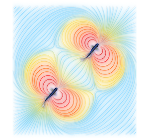
For the analysis, it is more convenient to express the velocity field (2) in the global Cartesian coordinate system. From Figure 1a, we deduce
 \begin{gather} \hat{\boldsymbol{e}}^{\boldsymbol{\rho}}_2(t) = {-}\hat{\boldsymbol{e}}^{\boldsymbol{\rho}}_1(t) = \frac{\Delta x(t) \hat{\boldsymbol{i}} + \Delta y(t) \hat{\boldsymbol{j}}}{\rho(t)}, \end{gather}
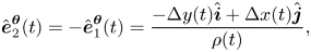 \begin{gather}\hat{\boldsymbol{e}}^{\boldsymbol{\theta}}_2 (t) = {-}\hat{\boldsymbol{e}}^{\boldsymbol{\theta}}_1 (t) = \frac{-\Delta y(t) \hat{\boldsymbol{i}} + \Delta x(t) \hat{\boldsymbol{j}}}{\rho(t)}, \end{gather}
where  $\Delta x(t) = x_1(t) - x_2(t)$ and
  $\Delta y(t) = y_1(t) - y_2(t)$, such that
  $\rho (t) = \sqrt {\Delta x(t)^2 + \Delta y(t)^2}$. Similarly, we can express the sines and cosines of the viewing angle in (2) in terms of individual orientations as
 \begin{gather} \cos{\theta_{\check{f},f}}(t) = \hat{\boldsymbol{v}}_{\check{f}}(t) \boldsymbol{\cdot} \hat{\boldsymbol{e}}^{\boldsymbol{\rho}}_{\check{f}}(t) = {\pm}\frac{\Delta x(t) \cos{\theta_{\check{f}}}(t) + \Delta y(t)\sin{\theta_{\check{f}}}(t)}{\rho(t)}, \end{gather}
 \begin{gather}\sin{\theta_{\check{f},f}}(t) = (\hat{\boldsymbol{v}}_{\check{f}}(t) \times \hat{\boldsymbol{e}}^{\boldsymbol{\rho}}_{\check{f}}(t)) \boldsymbol{\cdot} \hat{\boldsymbol{k}} = {\pm}\frac{\Delta y (t) \cos{\theta_{\check{f}}}(t)-\Delta x(t)\sin{\theta_{\check{f}}}(t)}{\rho(t)}, \end{gather}
where the plus (minus) sign is for  $f$ equal to 1 (2).
By replacing (3) and (4) into (2), we establish
 \begin{align} \boldsymbol{U}_{f}(\boldsymbol{r}_f(t)) & = \frac{r_{0,\check{f}}^2 v_{0,\check{f}}}{\rho(t)^{4}} [((\Delta x(t)^{2}- \Delta y(t)^{2})\cos{\theta_{\check{f}}}(t) + 2\Delta x(t)\Delta y(t)\sin{\theta_{\check{f}}}(t))\hat{\boldsymbol{i}} \nonumber\\ &\quad + ((\Delta y(t)^{2}-\Delta x(t)^{2})\sin{\theta_{\check{f}}(t)} + 2\Delta x(t)\Delta y(t)\cos{\theta_{\check{f}}(t)})\hat{\boldsymbol{j}}]. \end{align}
 To complete the model of the fish pair, we must prescribe governing equations for the orientation  $\theta _f(t)$,
  $f\in \{1,2\}$. Different from the work of Reference Filella, Nadal, Sire, Kanso and EloyFilella et al. (Reference Filella, Nadal, Sire, Kanso and Eloy2018), we employ a dynamic model that captures inherent delays in zebrafish to respond to visual or hydrodynamic input. Based on earlier models of social interaction, such as those by Reference Calovi, Lopez, Ngo, Sire, Chaté and TheraulazCalovi et al. (Reference Calovi, Lopez, Ngo, Sire, Chaté and Theraulaz2014, Reference Calovi, Lopez, Schuhmacher, Chaté, Sire and Theraulaz2015), we propose
 \begin{gather} \dot{\theta}_{f}(t) = \omega_{f}(t), \end{gather}
 \begin{gather}\mathrm{d}{\omega}_{f}(t) = {-}\eta_f(\omega_{f}(t)-\omega^{{\star}}_{f}(t)-{\varOmega}_{f}(t))\,\mathrm{d}t + \mathrm{d}N_f(t). \end{gather}
Here,  $\eta _f$ is the mean reversion rate that defines the characteristic time scale for fish to respond to external stimuli, thereby condensing neurological processes in decision-making and physical delays in reaction to external stimuli into a single damping coefficient per unit moment of inertia (in a kinematic model like in the work of Reference Filella, Nadal, Sire, Kanso and EloyFilella et al. (Reference Filella, Nadal, Sire, Kanso and Eloy2018),
  $\eta _f\rightarrow \infty$);
  $\omega ^{\star }(t)$ is the imposed turn rate from social interactions;
  ${\varOmega} _f(t)$ is the imposed turn rate owing to hydrodynamic interactions; and
  $N_f(t)$ is added noise in the form of a zero-mean stationary stochastic process that captures non-deterministic forcing from the surroundings (called ‘free will’ by Reference Filella, Nadal, Sire, Kanso and EloyFilella et al., 2018). All these contributions are linearly superimposed in the present model. The modelling choice of including reversion on the turn rate dynamics while assuming constant speed is a first approximation, motivated by earlier work that demonstrated the need of a rich dynamics for the turn rate to faithfully reproduce key elements of the behavioural phenotype (Reference Gautrais, Jost, Soria, Campo, Motsch, Fournier and TheraulazGautrais et al., 2009; Reference Mwaffo, Anderson, Butail and PorfiriMwaffo et al., 2015).
The response function  $\mathrm {\omega}_{f}^{\star}(t)$ accounts for social interactions, which primarily arise from visual cues and result in the tendency of the animals to align their bodies during swimming (schooling) and swim in the vicinity of others (shoaling), see, for example, the paper by Reference Miller and GerlaiMiller & Gerlai (Reference Miller and Gerlai2011). We write the response function for fish
  $f$, as originally proposed by Reference Calovi, Lopez, Ngo, Sire, Chaté and TheraulazCalovi et al. (Reference Calovi, Lopez, Ngo, Sire, Chaté and Theraulaz2014, Reference Calovi, Lopez, Schuhmacher, Chaté, Sire and Theraulaz2015), as
 \begin{equation} \omega^{{\star}}_{f}(t) = (1 + \cos{\theta_{f,\check{f}}}(t))(k_{v,f} v_{f}\sin{\phi_{f,\check{f}}}(t) + k_{p,f}\rho\sin{\theta_{f,\check{f}}}(t)), \end{equation}
where  $k_{v,f}$ and
  $k_{p,f}$ are gain parameters for alignment and attraction, respectively (Figure 1a), which summarize multisensory cues that underlie social response. These gains are the means by which one can simulate social behaviour, in the form of an animal orienting its swimming direction to align with and approach others.
The prefactor  $(1+\cos {\theta _{f,\check {f}}}(t))$ accounts for the cone of vision of zebrafish (Reference Pita, Moore, Tyrrell and Fernández-JuricicPita et al., 2015), which preferentially biases interactions toward animals that are swimming in front rather than those behind. As discussed by Reference Calovi, Lopez, Schuhmacher, Chaté, Sire and TheraulazCalovi et al. (Reference Calovi, Lopez, Schuhmacher, Chaté, Sire and Theraulaz2015), this prefactor ‘introduces a strong asymmetry between the force exerted by
  $f$ on
  $\check {f}$ and the one exerted by
  $\check {f}$ on
  $f$, and hence breaks the (Newtonian) action–reaction principle which is most familiar in the context of purely physical force, such as gravitation’.
The response function is such that the contribution to the imposed turn rate from the alignment rule tends to orient the swimming direction of  $f$ to align with
  $\check {f}$. Thus, it is zero when the animals are swimming in parallel (
 $\phi _{f,\check {f}}(t)=0$ or
  ${\rm \pi}$) and it is maximized in magnitude when they are swimming orthogonal to each other (
 $\phi _{f,\check {f}}(t)=\pm {\rm \pi}/2$ and
  $\theta _{f,\check {f}}(t)=0$). We choose to scale the attraction gain by the velocity, which is a constant, to acknowledge that faster fish will adjust their swimming direction more rapidly in response to external stimuli. However, the contribution from the attraction rule is such that
  $f$ will tend to correct its swimming direction to approach
  $\check {f}$: it is zero when
  $\theta _{f,\check {f}}(t)=0$ and maximized in magnitude when
  $\theta _{f,\check {f}}(t)=\pm {\rm \pi}/2$. In this model, alignment is taken to be independent of the relative distance between the animals, while attraction increases the further the animals are from one another. These approximations are expected to be valid when fish swim within approximately ten body lengths; otherwise, it may be appropriate to include a decay function that reduces the strength of the interaction for large distances (Reference Zienkiewicz, Barton, Porfiri and Di BernardoZienkiewicz et al., 2015b).
Within the finite-dipole framework, the turn rate imposed by hydrodynamic interactions  ${\varOmega} _f(t)$ arises from differences in the velocity experienced by each vortex comprising the dipole of fish
  $f$. Thus, in the far-field limit, the gradient of streamwise velocity in the direction orthogonal to
  $\hat {\boldsymbol{v}}_f$ induces the hydrodynamic turning
 \begin{equation} {\varOmega}_{f}(t) = {-} \hat{\boldsymbol{v}}_{f}(t) \boldsymbol{\cdot} [ \boldsymbol{\nabla} \boldsymbol{U}_{f}(\boldsymbol{r}_{f}(t)) \hat{\boldsymbol{v}}_{f}^{\boldsymbol{\perp}}(t)], \end{equation}
where  $\hat {\boldsymbol{v}}_{f}^{\boldsymbol{\perp}} (t)=\hat {\boldsymbol{k}}\times \hat {\boldsymbol{v}}_{f}(t)$ is the unit vector orthogonal to
  $\hat {\boldsymbol{v}}_f(t)$ forming a local right-handed coordinate system and
  $\boldsymbol {\nabla }$ is the gradient operator in the global coordinate system. With respect to the paper by Reference Filella, Nadal, Sire, Kanso and EloyFilella et al. (Reference Filella, Nadal, Sire, Kanso and Eloy2018), we note the difference in sign between (8) and (5) therein, which arises from our choice to work with transverse versus aligned dipoles, that is, T-dipoles instead of A-dipoles, as defined by Reference Kanso and TsangKanso & Tsang, 2014. One can verify that the sign is indeed negative by considering a fish swimming in the
  $x$-direction (
 $\theta _f=0$,
  $\hat {\boldsymbol{v}}_f=\hat {\boldsymbol{i}}$, and
  $\hat {\boldsymbol{v}}_{f}^{\boldsymbol{\perp} }=\hat {\boldsymbol{j}}$) in a shear flow (
 $\boldsymbol {U}_f=\alpha Y \hat {\boldsymbol{i}}$ with
  $\alpha >0$); in this case, the turn rate in (8) is
  $-\alpha$ such that the fish will turn clockwise, as one would expect also based on the work of Reference Tchieu, Kanso and NewtonTchieu et al. (Reference Tchieu, Kanso and Newton2012). For completeness, we report results also for the case of A-dipoles in the supplementary material. By using the expression of the velocity
  $\boldsymbol {U}_{f}(\boldsymbol {r}_{f}(t))$ in (5), along with the Cartesian representation of
  $\hat {\boldsymbol{v}}_{f}^{\boldsymbol{\perp}} (t)$ and
  $\hat {\boldsymbol{v}}_{f}(t)$, we establish
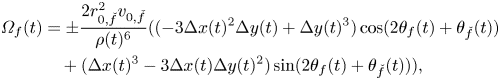 \begin{align} {\varOmega}_f(t) & = {\pm}\frac{2 r_{0, \check{f}}^{2} v_{0,\check{f}}}{\rho(t)^6}(({-}3 \Delta x(t)^2 \Delta y(t) + \Delta y(t)^3) \cos(2 \theta_{f}(t) + \theta_{\check{f}}(t))\nonumber\\ &\quad + (\Delta x(t)^3 - 3 \Delta x(t) \Delta y(t)^2) \sin(2\theta_{f}(t) + \theta_{\check{f}}(t))), \end{align}
where the minus (plus) sign is for  $f$ equal to 1 (2). Comparing (9) with (7), we register a contrasting dependence on the distance between the two fish, whereby social interaction linearly increases with
  $\rho (t)$, while the hydrodynamic turning decreases with
  $\rho (t)^3$.
Added noise in (6b) captures the uncertainty in the behaviour of the animal, which may not necessarily balance between social and hydrodynamic interactions. Zebrafish locomotion is characterized by a unique burst-and-coast swimming style in which ‘fish move forward (burst) in a single motion and glide (coast) to a slow speed, or stop from which they burst forward again’ (Reference Kalueff, Gebhardt, Stewart, Cachat, Brimmer and ChawlaKalueff et al., 2013). This swimming style contributes to a rich repertoire of locomotory patterns, which include sudden U- and C-turns that alternate with instances of straight swimming (Reference Kalueff, Gebhardt, Stewart, Cachat, Brimmer and ChawlaKalueff et al., 2013). As a result, uncertainty in turn rate dynamics cannot be captured by Gaussian white noise (that is, increments of a Wiener process), as traditionally advocated for other swimming animals (Reference Gautrais, Jost, Soria, Campo, Motsch, Fournier and TheraulazGautrais et al., 2009).
This issue has been addressed by Reference Mwaffo, Anderson, Butail and PorfiriMwaffo et al. (Reference Mwaffo, Anderson, Butail and Porfiri2015) by modelling added noise as the sum of two terms: (i) a Wiener process  $\sigma _f W(t)$, where
  $W(t)$ is a standard Wiener process and
  $\sigma _f$ is a positive constant (note that for a standard Wiener process,
  $\mathrm {d}W(t)\sim \mathcal {N}(0,\mathrm {d}t)$, where
  $\mathcal {N}(\mu ,\sigma ^2)$ is a normal distribution with mean
  $\mu$ and variance
  $\sigma ^2$, so that multiplying by
  $\sigma _f$ scales the variance of the normal distribution by
  $\sigma _f^2$), and (ii) a compound Poisson process
  $J_f(t)=\sum _{k=1}^{P_f(t)}Z_{f,k}$, where
  $P_f(t) - P_f(s)$, for
  $s\leq t$, is a Poisson random variable with parameter
  $\lambda _f(t-s)$, and
  $Z_{f,k}\sim \mathcal {N}(0,\gamma _f^2)$ (note that the increment in the compound Poisson process can be written as
  $\mathrm {d}J_f(t)=Z\mathrm {d}P_f(t)$, where
  $Z\sim \mathcal {N}(0,\gamma _f^2)$ and
  $\mathrm {d}P_f(t)\sim \mathcal {B}(\lambda _f\,\mathrm {d}t)$,
  $\mathcal {B}(q)$ being a Bernoulli distribution with parameter
  $q$). The Wiener process represents the baseline uncertainty with animal locomotion. The compound Poisson process allows the capture of jumps in the turn rate dynamics, which are associated with C- and U-turns. A sample video of a zebrafish pair swimming is included as a supplementary movie. Overall, added noise is modelled through three independent parameters:
  $\sigma _f$, setting a baseline activity for the animal;
  $\lambda _f$, quantifying the frequency of the jumps; and
  $\gamma _f$, measuring the strength of the jumps.
In light of the choice of the form of added noise, (6b) can be viewed as a jump reverting mean diffusion process (Reference TankovTankov, 2003), in which the turn rate relaxes toward a time-varying mean, given by the sum of the turn rates imposed by social and hydrodynamic interactions in (7) and (8), respectively. The original model by Reference Filella, Nadal, Sire, Kanso and EloyFilella et al. (Reference Filella, Nadal, Sire, Kanso and Eloy2018) has neither the feature of reversion nor the presence of jumps. Hence, at every time, the turn rate of each fish matches the sum of the turn rates imposed by social and hydrodynamic interactions, subject to added Gaussian white noise (note that in the model by Reference Filella, Nadal, Sire, Kanso and EloyFilella et al. (Reference Filella, Nadal, Sire, Kanso and Eloy2018),  $\omega _{f}(t)=\omega ^{\star }_{f}(t)+ \varOmega_{f}(t) +\sigma _f ({\mathrm {d}W(t)}/{\mathrm {d}t})$, where
  $\sigma _f$ has units
  $\mathrm {rad\,s^{-1}}$ rather than
  $\mathrm {rad\,s^{-{3/2}}}$ as in our study).
3. Analytical Insight into the Model
Predicting the behaviour of a zebrafish pair requires the time integration of (1) and (6). While the general mathematical treatment of this system may not be feasible, important insight can be gathered by examining its linearized dynamics about salient configurations that have previously been documented (Reference De Bie, Manes and KempDe Bie et al., 2020; Reference Kato, Nakagawa, Ohkawa, Muramoto, Oyama, Watanabe and SugitaniKato et al., 2004; Reference Laan, Gil de Sagredo and de PolaviejaLaan et al., 2017; Reference Perna, Grégoire and MannPerna et al., 2014; Reference Saadat, Berlinger, Sheshmani, Nagpal, Lauder and Haj-HaririSadaat et al., 2021). To further simplify the problem, we assume the two fish to be identical, such that  $r_{0,1}=r_{0,2}= r_{0}$,
  $v_{0,1}=v_{0,2} =v_0$,
  $k_{p,1}=k_{p,2}=k_p$,
  $k_{v,1}=k_{v,2}=k_v$,
  $\eta _1=\eta _2=\eta$,
  $\sigma _1=\sigma _2=\sigma$,
  $\lambda _1=\lambda _2=\lambda$ and
  $\gamma _1=\gamma _2=\gamma$.
Following standard practice in the literature on synchronization of coupled dynamical systems (Reference Pikovsky, Kurths, Rosenblum and KurthsPikovsky et al., 2003), we decompose the dynamics of the fish pair into average and error dynamics. The former captures the evolution of the centre of mass of the pair and of the average orientation, whereas the latter describes changes in relative distance and orientation. Hence, we write
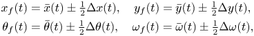 \begin{align} x_f(t) &= \bar{x}(t)\pm\tfrac{1}{2}\Delta x(t), \quad y_f(t) = \bar{y}(t)\pm\tfrac{1}{2}\Delta y(t),\notag\\ \theta_f(t) &= \bar{\theta}(t)\pm\tfrac{1}{2}\Delta \theta(t), \quad \omega_f(t) = \bar{\omega}(t)\pm\tfrac{1}{2}\Delta \omega(t), \end{align}
where the plus (minus) sign is for  $f$ equal to 1 (2), a superimposed bar indicates the average dynamics and the symbol
  $\Delta$ is consistently used to label relative dynamics.
By using this coordinate transformation, we consider the eight-dimensional state variable  $z(t)=[\bar {x}(t),\bar {y}(t),\bar {\theta }(t),\bar {\omega }(t),\Delta x(t),\Delta y(t),\Delta \theta (t),\Delta \omega (t)]^{\mathrm {T}}$, where
  $\mathrm {T}$ indicates matrix transposition. The time evolution of the state is given by
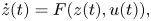 \begin{equation} \dot{z}(t) = F(z(t),u(t)), \end{equation}
where  $u(t)\in \mathbb {R}^2$ encapsulates added noise to the turn rate dynamics of the animals and the nonlinear function
  $F:\mathbb {R}^8\times \mathbb {R}^2\rightarrow \mathbb {R}^8$ captures the first-order dynamics of the turn rate in (6b) along with the coupling between the state variables of the two fish through the advection velocity (2), social interactions (7) and hydrodynamic interactions (8).
The class of nominal solutions about which we perform a linearization is part of the schooling patterns identified by Reference Filella, Nadal, Sire, Kanso and EloyFilella et al. (Reference Filella, Nadal, Sire, Kanso and Eloy2018), wherein fish swim along the same, constant direction, that is,  $\Delta \theta (t)=0$ and
  $\bar {\theta }(t)=\theta _c$ for some
  $\theta _c$. Fish will follow a straight line (
 $\Delta \omega (t)=0$ and
  $\bar {\omega }(t)=0$) and rigidly translate one with respect to each other, as shown in Figure 1b. In this in-line swimming pattern (sometimes called ‘tandem’), one fish follows the other, such that
  $\Delta x(t)=d\cos \theta _c$ and
  $\Delta y(t)=d\sin \theta _c$, where
  $d$ is the constant distance between the fish. Without loss of generality, we set
  $\theta _c=0$, such that the
  $x$-axis of the Cartesian coordinate system is aligned with the schooling direction.
It is easy to verify that for any choice of  $d$, in-line swimming constitutes a nominal solution of (11) in the absence of added noise. Specifically, both the imposed turn rates owing to social and hydrodynamic interactions in (7) and (8) are identically zero, such that the orientation of each fish remains constant (
 $\hat {\boldsymbol{v}}_f(t)=\hat {\boldsymbol{i}}$). With respect to the positional coordinates, we observe that
  $\boldsymbol {U}_f(\boldsymbol {r}_f(t))=({r_0^2 v_0}/{d^2})\hat {\boldsymbol{i}}$ for
  $f\in \{1,2\}$, such that each fish will be subject to the same advective velocity, thereby preserving the relative configuration. The centre of mass of the pair will move at a constant speed given by
  $v_0(1+{r_0^2}/{d^2})$, which yields the increase in speed arising from hydrodynamic interaction observed through simulations on large groups (Reference Filella, Nadal, Sire, Kanso and EloyFilella et al. 2018).
The homogeneous, linearized dynamics of the system is informative of the local stability of the in-line configuration. By taking the gradient of the nonlinear vector field in (11) and evaluating it at the nominal solution, we obtain the following state matrix describing the evolution of perturbations with respect to the nominal, in-line solution:
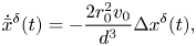 \begin{gather} \dot{\bar{x}}^{\delta}(t) = {-}\frac{2 r_0^2 v_0}{d^3}\Delta x^{\delta}(t), \end{gather}
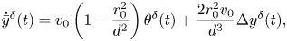 \begin{gather}\dot{\bar{y}}^{\delta}(t) = v_0\left(1-\frac{r_0^2}{d^2}\right) \bar{\theta}^{\delta}(t) + \frac{2 r_0^2 v_0}{d^3}\Delta y^{\delta}(t), \end{gather}
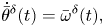 \begin{gather}\dot{\bar{\theta}}^{\delta}(t) = \bar{\omega}^{\delta}(t), \end{gather}
 \begin{gather}\dot{\bar{\omega}}^{\delta}(t) = {-}k_p\eta d\bar{\theta}^{\delta}(t)-\eta\bar{\omega}^{\delta}(t) + k_p\eta\Delta y^{\delta}(t) + \left(-\frac{\eta r_0^2v_0}{d^3} + \frac{k_p \eta d }{2} + k_v \eta v_0 \right)\Delta \theta^{\delta}(t), \end{gather}
 \begin{gather}\dot{\Delta x}^{\delta}(t) = 0, \end{gather}
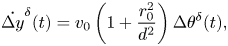 \begin{gather}\dot{\Delta y}^{\delta}(t) = v_0\left(1 + \frac{r_0^2}{d^2}\right)\Delta \theta^{\delta}(t), \end{gather}
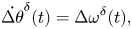 \begin{gather}\dot{\Delta \theta}^{\delta}(t) = \Delta \omega^{\delta}(t),\end{gather}
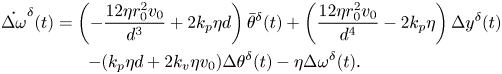 \begin{gather} \dot{\Delta \omega}^{\delta}(t) = \left(-\frac{12\eta r_0^2v_0}{d^3} + 2 k_p \eta d\right)\bar{\theta}^{\delta}(t) + \left(\frac{12\eta r_0^2v_0}{d^4}-2k_p\eta\right)\Delta y^{\delta}(t) \notag\\ -(k_p\eta d + 2 k_v \eta v_0)\Delta \theta^{\delta}(t)-\eta \Delta \omega^{\delta}(t). \end{gather}
Here and henceforth, a superscript  $\delta$ identifies perturbations with respect to the nominal solution.
Equation (12) demonstrates several interesting features of the model. First, perturbations on the position of the centre of mass do not enter the dynamics of any of the other state variables. Second, the relative distance along the schooling direction remains constant, independent of any other state variable. Third, the perturbation on the relative distance  $\Delta y^{\delta }(t)$ depends only on the relative rotation
  $\Delta \theta ^{\delta }(t)$. Fourth, the response of the fish pair is asymmetric, owing to the presence of social interactions which are sensitive to the relative orientation of the animals (leading versus trailing fish); asymmetry is evident in the turn rate dynamics by combining (12d) and (12h) to obtain governing equations for
  $\omega _1^{\delta }(t)$ and
  $\omega _2^{\delta }(t)$.
To further clarify the structure of the system, we perform a coordinate transformation that accounts for the specific nature of in-line swimming. Specifically, we define  $\bar {\theta }_{\star }^{\delta }(t)=\bar {\theta }^{\delta }(t)-{\Delta y^{\delta }(t)}/{d}$ to filter out rigid-body motion in the definition of the average angle; in fact, in-line swimming would not be affected if both fish moved along the
  $y$-axis while rotating their bodies to preserve straight swimming. Consistently, we define
  $\bar {\omega }_{\star }^{\delta }(t)=\dot {\bar {\theta }}_{\star }^{\delta }(t)$. By using these variables in (12) and ordering the components of the state vector as
  $z^{\delta }(t)=[\bar {x}^{\delta }(t),\bar {y}^{\delta }(t),\Delta x^{\delta }(t),\Delta y^{\delta }(t),\bar {\theta }_{\star }^{\delta }(t),\bar {\omega }_{\star }^{\delta }(t), \Delta \theta ^{\delta }(t),\Delta \omega ^{\delta }(t)]^{\mathrm {T}}$, we can write the state matrix of the system in the following block-triangular form:
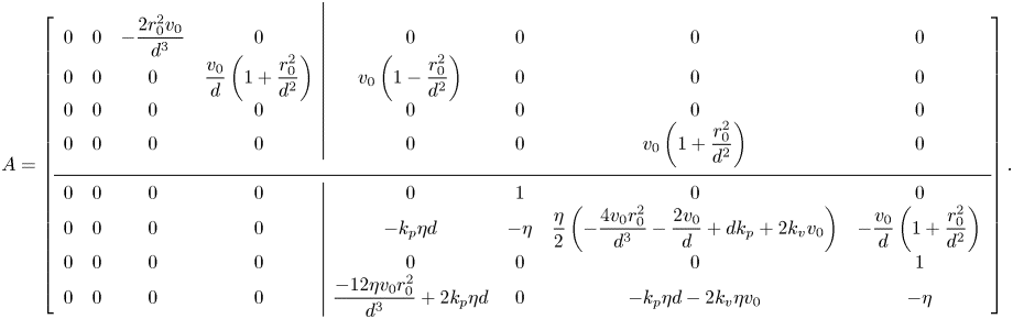
The stability of in-line swimming to external perturbations is ascertained by examining the spectrum of the four-by-four block on the bottom diagonal,  $A_{22}$. In-line swimming is asymptotically stable if, and only if, this sub-matrix is Hurwitz. If
  $A_{22}$ is Hurwitz, the orientations converge to a common value (
 $\Delta \theta ^{\delta }(t),\Delta \omega ^{\delta }(t)\rightarrow 0$), such that the two fish swim along a straight line (
 $\bar {\theta }_{\star }^{\delta }(t),\bar {\omega }_{\star }^{\delta }(t) \rightarrow 0$). The other blocks have no role on stability, whereby the location of the centre of mass and the relative distance
  $\Delta x^{\delta }(t)$ are inconsequential with respect to in-line swimming, and
  $\Delta y^{\delta }(t)$ converges to a constant value that depends on the common orientation attained by the fish pair.
While a precise evaluation of the stability of in-line swimming requires the calculation of the spectrum of  $A_{22}$, important insight can be gathered from the application of the Routh–Hurwitz criterion. Briefly, application of the criterion requires the construction of an ancillary table of coefficients, which is computed from the coefficients of the characteristic polynomial (Reference MeinsmaMeinsma, 1995). By counting the number of sign changes in the first columns of this table, it is possible to exactly count the number of eigenvalues with positive real part. Going through simple algebra, we obtain the following expression for the first column of the Routh table
  $R=\{R_4,R_3,\ldots ,R_0\}$:
 \begin{gather} R_4 = 1, \end{gather}
 \begin{gather}R_3 = 2\eta, \end{gather}
 \begin{gather}R_2 = {-}\frac{v_0 (d^2 + r_0^2) (k_p d^4 -6 r_0^2 v_0)}{d^6} + \eta (k_p d + k_v v_0) + \eta^2, \end{gather}
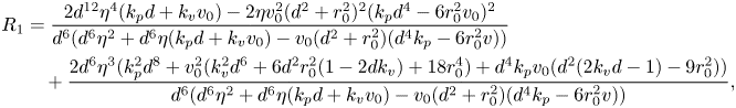 \begin{align} R_1& = \frac{2 d^{12} \eta^4 ( k_p d + k_v v_0)-2 \eta v_0^2 (d^2 + r_0^2)^2 (k_p d^4 -6 r_0^2 v_0)^2}{d^6 (d^6 \eta ^2 + d^6 \eta (k_p d + k_v v_0)-v_0 (d^2 + r_0^2) (d^4 k_p-6 r_0^2 v))} \nonumber\\ &\quad + \frac{2 d^6 \eta^3 (k_p^2 d^8 + v_0^2 (k_v^2 d^6 + 6 d^2 r_0^2 (1-2 d k_v) + 18 r_0^4) + d^4 k_p v_0 (d^2 (2 k_v d -1)-9 r_0^2))}{d^6 (d^6 \eta ^2 + d^6 \eta (k_p d + k_v v_0)-v_0 (d^2 + r_0^2) (d^4 k_p-6 r_0^2 v))}, \end{align}
 \begin{equation} R_0 = \frac{2 \eta^2 v_0 \left((d^2 + 5 r_0^2)d^4k_p + 6d^3 r_0^2v_0k_v-6\left(d^2 + 2r_0^2\right)r_0^2v_0\right)}{d^6}. \end{equation}
 In general, it is difficult to tell the sign of the terms in (14), but several interesting limit cases can be explored. For example, for a sufficiently large  $d$, we discover that there are no sign changes (all terms being positive), which demonstrates that in-line swimming is asymptotically stable for sufficiently large separation distances. However, for small values of
  $d$, there is one sign change (
 $R_1\rightarrow -\infty$), which indicates the presence of one eigenvalue with a positive real part.
We can also examine the case in which fish interact only hydrodynamically, such that both  $k_p$ and
  $k_v$ approach zero. In this case, we register at least one sign change, whereby
  $R_0=-{12 \eta ^2 r_0^2 v_0^2 (d^2+2 r_0^2)}/$
  ${d^6}<0$. This suggests that visual cues are needed to ensure the stability of in-line swimming, which supports the simulation results in Figure 7b of Reference Tchieu, Kanso and NewtonTchieu et al. (Reference Tchieu, Kanso and Newton2012) and echo analytical predictions on large-head microswimmers (Reference Kanso and TsangKanso & Tsang, 2015) and suspensions of phoretic particles (Reference Kanso and MichelinKanso & Michelin, 2019).
Another interesting case is the limit of large values of  $\eta$, which is reminiscent of the set-up by Reference Filella, Nadal, Sire, Kanso and EloyFilella et al. (Reference Filella, Nadal, Sire, Kanso and Eloy2018); in this case,
  ${R_0}/{\eta ^2}=-6(d^2+2r_0^2)r_0^2v_0+(d^2 +5 r_0^2)d^4k_p+6d^3 r_0^2v_0k_v>0$ is the necessary and sufficient condition for the matrix to be Hurwitz, because all the other terms are positive. For small values of
  $d$, the leading term is
  $-12r_0^4v_0$, which confirms the instability of in-line swimming, unless
  $k_v$ and
  $k_p$ are sufficiently large to dominate
  $R_0$. Predictably, large values of
  $k_v$ and
  $k_p$ will favour stability for any choice of
  $d$. Should hydrodynamic interactions be dismissed by setting
  $r_0=0$, we would always obtain asymptotic stability.
Another swimming pattern that is often considered in the literature is side-by-side swimming (Reference De Bie, Manes and KempDe Bie et al., 2020; Reference Kato, Nakagawa, Ohkawa, Muramoto, Oyama, Watanabe and SugitaniKato et al., 2004; Reference Laan, Gil de Sagredo and de PolaviejaLaan et al., 2017; Reference Perna, Grégoire and MannPerna et al., 2014), where the fish swim parallel to each other with  $\Delta x(t)=-d\sin \theta _c$ and
  $\Delta y(t)=d\cos \theta _c$. For the present model, this swimming pattern does not constitute a nominal solution: hydrodynamic interactions will have an equivalent effect as alignment and attraction, thereby causing the fish to approach one another.
The analysis presented thus far relies on the classical finite-dipole paradigm of Reference Tchieu, Kanso and NewtonTchieu et al. (Reference Tchieu, Kanso and Newton2012) to study fish schooling, which was later referred to as the transverse (T) dipole to distinguish from the aligned (A) dipole (Reference Kanso and TsangKanso & Tsang, 2014). As noted by Reference Kanso and TsangKanso & Tsang (Reference Kanso and Tsang2014), the two models only differ in ‘how an individual dipole aligns itself with the local flow gradient’. The T-dipole aligns itself based on the difference in the flow velocity in the direction transverse to the dipole, while the A-dipole aligns itself according to the difference in the flow velocity along the dipole direction, similar to the active swimmers in microfluidic devices considered by Reference Brotto, Caussin, Lauga and BartoloBrotto et al. (Reference Brotto, Caussin, Lauga and Bartolo2013). For completeness, we report analytical insight into the model also for the case of A-dipoles in the supplementary material.
4. Experimental Data and Model Calibration
We calibrated the model using experimental data from a previous study (Reference Zienkiewicz, Barton, Porfiri and Di BernardoZienkiewicz et al., 2015a); the same dataset was also used by Reference Butail, Mwaffo and PorfiriButail et al. (Reference Butail, Mwaffo and Porfiri2016) and is included in the supplementary material. The dataset contains  $17$ different pairs of adult zebrafish with an average body length (BL) of
  $30\ \mathrm {mm}$ swimming in a circular arena of
  $0.9\ \mathrm {m}$ diameter and water depth of
  $0.1\ \mathrm {m}$. The shallow depth encouraged the fish to swim in a quasi-two dimensional plane. Fish motion was filmed at
  $30\ \mathrm {frames\,s^{-1}}$ for
  $20$ min, and a multi-target tracking system (Reference Ladu, Butail, Macrí and PorfiriLadu et al., 2014) was used to track the centroids of each individual. The first
  $10\ \mathrm {min}$ were treated as a habituation phase, in which the animals explored the novel tank and acclimatized to the environment.
The last  $10$ min of the videos were used for the analysis. Each pair of experimental trajectory data consists of positions
  $\boldsymbol {r}_{f}(t)$ and orientations
  $\theta _{f}(t)$ in the instantaneous direction of motion of the two animals sampled at a time step
  $\Delta t=1/30\ \mathrm {s}$. We filtered the data in two steps. Time windows where the two fish were closer than half a BL from each other were removed to avoid diving instances, which would violate the assumption of planar swimming. To mitigate the effect on unmodelled hydrodynamic interactions with the walls, we also removed instances when either fish swam closer than two BLs to the wall. Overall, these pre-processing steps curtailed approximately half of the dataset.
This same dataset was also used to validate the predictions of the model, by evaluating salient metrics of collective behaviour that emerge within the pair. Specifically, we considered the average polarization, which measures the relative orientation of the pair:  $\mathrm {Pol} = ({1}/{T})\int _{0}^{T} ({\|\hat {\boldsymbol{v}}_{1}(t)+\hat {\boldsymbol{v}}_{2}(t)\|}/{2})\,\mathrm {d}t$, where
  $T$ is the duration of the observation (Reference Calovi, Lopez, Ngo, Sire, Chaté and TheraulazCalovi et al., 2014). A polarization value of one indicates that the swimming directions of both fish are always aligned during he observation window, whereas a value of zero identifies that the animals are swimming in opposite directions. While polarization helps to quantify schooling, it does not distinguish between in-line and side-by-side swimming, which we capture through a pursuit index defined as
  $\mathrm {PI} = ({1}/{T}) \int _0^T({(\hat {\boldsymbol{v}}_{1}(t)+\hat {\boldsymbol{v}}_{2}(t)) \boldsymbol {\cdot } (\boldsymbol {r}_{1}(t)-\boldsymbol {r}_{2}(t))}/{2 \rho (t)})\,\mathrm {d}t$. A value of
  $1$ (
$1$ ( $-1$) indicates in-line swimming, with the first (second) fish swimming in front of the second (first) fish. A zero value corresponds to the pair swimming side-by-side. The average inter-individual distance between the pair of fish,
  $\mathrm {Dist}=({1}/{T})\int _{0}^{T}|\rho (t)|\,\mathrm {d}t$, is used to quantify their shoaling tendency, that is, their preference to stay close to one another. Finally, we measured the average speed of the centre of mass
  $\mathrm {Speed}=({1}/{T}) \int _0^T({\|\dot {\boldsymbol {r}}_{1}(t)+\dot {\boldsymbol {r}}_{2}(t)\|}/{2})\,\mathrm {d}t$ to further detail the effect of interactions on locomotion.
For each fish, we identified eight model parameters (characteristic length,  $r_0$; speed,
  $v_0$; baseline activity,
  $\sigma _f$; reversion rate,
  $\eta _f$; jump frequency,
  $\lambda _f$; jump intensity,
  $\gamma _f$; and attraction and alignment gains,
  $k_{p,f}$ and
  $k_{v,f}$, respectively) from the equations of motion (1) and (6). We performed the identification in two sequential steps. First, we calibrated characteristic length,
  $r_0$, and speed,
  $v_0$, by minimizing the sum-square-error cost function (SSECF) calculated from the experimentally measured speed and the speed in (1), defined as
  $\mathrm {SSECF} = \sum _{k\in \mathrm {Data}_f}(\|\dot {\boldsymbol {r}}_f(t_k)\|-\|v_f \hat {\boldsymbol{v}}_f(t_k)+\boldsymbol {U}_f(\boldsymbol {r}_f(t_k))\|)^2$, where ‘
 $\mathrm {Data}_f$’ identifies the subset of indices that remain after the removal presented above for fish
  $f$. The optimization was solved by constraining each parameter within a physically plausible range. Specifically, based on prior data on fish swimming in isolation and the typical body length of a zebrafish (Reference Ladu, Butail, Macrí and PorfiriLadu et al., 2014), we selected
  $v_f \in [0,0.30]\ \mathrm {m}\ \mathrm {s}^{-1}$ and
  $r_f \in [0,30]\ \mathrm {mm}$. Calibrated parameters are presented in Figure 2a,b.

Figure 2. Calibrated model parameters: (a) characteristic length; (b) speed; (c) baseline activity; (d) mean reversion rate; (e) jump frequency; (f) jump intensity; (g) gain parameter for attraction; and (h) gain parameter for alignment. The coloured area in each violin plot is the probability density and coloured circles are individual calibrations. Thick grey bars indicate first and third quartiles; thin grey bars identify minimum and maximum values; and white circles are the median. Calibrated parameters for each fish are reported in the supplementary material.
Second, we identified the remaining six parameters  $\Theta _{f}=[\sigma _{f},\eta _{f},\lambda _{f},\gamma _{f},k_{p,f},k_{v,f}]^{\mathrm {T}}$ using a maximum likelihood approach on the turn rate dynamics in (6b). The maximum likelihood estimation was subject to further data preprocessing, whereby we removed instances when fish were swimming approximately in-line (
 $\mathrm {AI}>0.75$); at these instances, the prefactor in the social interaction (7) would cause excessively small values of the response function, which would challenge robust identification.
Hence, we estimated the model parameters by minimizing the sum of negative logarithms of the likelihood function  $\mathcal {L}(\omega _{f}(t)|\omega _{f}(t-\Delta t),\Theta _{f})$ over experimental time-series using the
  $\texttt {FMINCON}$ function in
  $\mathrm {MATLAB}$ (Reference Butail, Mwaffo and PorfiriButail et al., 2016). The likelihood function was constructed as the sum of two normal probability distributions associated with the two forms of added noise,
 \begin{align} \mathcal{L}(\omega_{f}(t)|\omega_{f}(t-\Delta t),\Theta_{f}) & = (1-\lambda_{f} \Delta t) H(\omega_{f}(t),\mu_{f}(\omega_{f}(t-\Delta t), \Delta t),\mathrm{var}_{f}(\Delta t)) \nonumber\\ &\quad + \lambda_{f} \Delta t H(\omega_{f}(t),\mu_{f}(\omega_{f}(t-\Delta t), \Delta t),\mathrm{var}_{f}(\Delta t) + \gamma_{f}), \end{align}
where
 \begin{gather} \mu_{f}(\omega_{f}(t-\Delta t), \Delta t) = \omega_{f}(t-\Delta t)\, \textrm{e}^{-\eta_f \Delta t} + (\omega_{f}^{{\star}}(t-\Delta t) + {\varOmega}_{f}(t-\Delta t)) (1-\textrm{e}^{-\eta_f \Delta t}), \end{gather}
 \begin{gather}\mathrm{var}_{f}(\Delta t) = \frac{\sigma_f^2}{2\eta_f}(1-\textrm{e}^{{-}2\eta_f \Delta t}), \end{gather}
and  $H(\bullet ,\mu ,\sigma ^2)$ is the probability mass function of
  $\mathcal {N}(\mu ,\sigma ^2)$.
Based on the social model of Reference Butail, Mwaffo and PorfiriButail et al. (Reference Butail, Mwaffo and Porfiri2016), we constrained the parameter ranges for the search as follows. First, we set  $\eta _f \in [1,2] \ \mathrm {s}^{-1}$,
  $\sigma _f \in [1,5] \ \mathrm {rad}\ \mathrm {s}^{-3/2}$ and
  $\gamma _f \in [1,5] \ \mathrm {rad}\ \mathrm {s}^{-1}$. Then, we explored the range in jump frequency of
  $\lambda _f \in [0.9,1.1]\lambda _{0,\kern0.05em f}$, where
  $\lambda _{0,\kern0.05em f}$ was an estimate of the frequency of extreme events in the time-series, defined as the ratio between the number of time steps above three standard deviations from the mean of the turn rate and the total number of time steps. With respect to interactions parameters, we explored the broad range
  $k_{p,f} \in [0,100] \ \mathrm {rad}\ \mathrm {m}^{-1}\ \mathrm {s}^{-1}$ and
  $k_{v,f} \in [0,100] \ \mathrm {rad}\ \mathrm {m}^{-1}$ to capture inter-individual variability in social behaviour.
5. Results and Discussion
By applying the calibration procedure explained above, we obtained the complete set of calibrated parameters, as shown in Figure 2. The values of  $r_0$ were one order of magnitude less than the animal body length (
 $r_0=3.1\pm 3.2\ \mathrm {mm}$), which corresponded to the typical tail beat amplitude of a cruising zebrafish (Reference Gazzola, Argentina and MahadevanGazzola et al., 2014). The self-propulsion speed ranged from 2BL to 6BL per second (
 $v_0=0.094\pm 0.027\ \mathrm {m\,s^{-1}}$), which suggested variability among animals with respect to their locomotion. Interestingly, these two variables were highly correlated, such that larger distances between vortices comprising the dipole will be accompanied by larger speeds, thus implying larger values of the vortices’ circulation, see Table 1. This trend was analogous to the relationship between tail beat amplitude and the circulation of vortices shed during tail beating in the real experiments by Reference Mwaffo, Zhang, Cruz and PorfiriMwaffo et al. (Reference Mwaffo, Zhang, Cruz and Porfiri2017).
Table 1. Coefficient of determination ( $R$) and associated
  ${p}$-value in parentheses between model variables. Significant correlations at a level of
  $0.05$ are indicated in bold (should one correct for multiple comparisons using a conservative Bonferroni correction, some significant correlations would become trends).
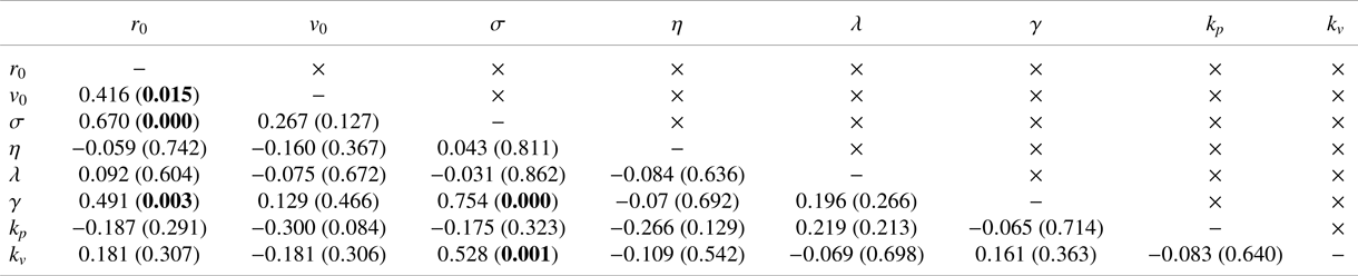
The baseline activity ( $\sigma =1.66\pm 0.61\ \mathrm {rad\, s^{-3/2}}$), mean reversion rate (
 $\eta =1.77\pm 0.32\ \mathrm {s^{-1}}$), jump frequency (
 $\lambda = 0.64\pm 0.12\ \mathrm {s^{-1}}$), jump intensity (
 $\gamma = 2.63\pm 0.77\ \mathrm {s^{-1}}$), and gain parameters for attraction (
 $k_p = 3.08\pm 3.43\ \mathrm {rad\,m^{-1}\,s^{-1}}$) and alignment (
 $k_v = 18.12\pm 13.12\ \mathrm {rad\,m^{-1}}$) were comparable with those of Reference Butail, Mwaffo and PorfiriButail et al. (Reference Butail, Mwaffo and Porfiri2016), which did not include a model of hydrodynamic coupling. These parameter values were not all independent of each other (Table 1). We determined a positive relationship between baseline activity and jump intensity, which suggested that animals exhibiting higher activity levels also displayed stronger bursts. We also recorded a positive correlation between
  $r_0$ and both the noise intensities,
  $\sigma$ and
  $\gamma$, which suggested that larger animals will tend to be more active and display more pronounced body movements during C- and U-turns. Finally, we discovered that the alignment gain was positively correlated with the baseline activity, which suggested that more active animals might exhibit a stronger social response, perhaps pointing at a deeper association between locomotory activity and social response that might be mediated by stress (Reference Kalueff, Gebhardt, Stewart, Cachat, Brimmer and ChawlaKalueff et al., 2013).
Overall, the extent to which hydrodynamic interactions improve the quality of the fit can be ascertained using the Akaike information criterion (Reference AkaikeAkaike, 1998). Specifically, for the present model in (6b), this quantity is equal to  $52.10\pm 33.33$. Should we compute the same for the model by Reference Butail, Mwaffo and PorfiriButail et al. (Reference Butail, Mwaffo and Porfiri2016), which excluded hydrodynamic interactions, we would obtain a strikingly similar result of
  $46.74 \pm 32.54$. Hence, accounting for hydrodynamic interactions does not lead to a tangible improvement on the fit of the turn rate, although it allows the capture of speed-based interactions that would be otherwise neglected. Evidence in favour of the existence of speed-based interactions has been documented in a number of experimental studies on freshwater fish (see, for example, Reference Herbert-Read, Perna, Mann, Schaerf, Sumpter and WardHerbert-Read et al., 2011; Reference Katz, Tunstrøm, Ioannou, Huepe and CouzinKatz et al., 2011), but their connection to hydrodynamics has remained elusive. The supplementary material contain calibrated model parameters for A-dipoles, which are highly comparable to those presented herein.
To demonstrate the model predictive power, we performed a series of in silico experiments, which employed the calibrated parameters from Figure 2; a sample video is included as a supplementary movie. This analysis aimed to ascertain whether the model predicts equivalent statistical outcomes to real experiments, thereby allowing for partial replacement of animal trials. We ran the model  $17$ times to mirror experimental observations, using identical parameters for each fish in the pair (drawn from normal distributions approximating those in Figure 2) and random initial conditions (orientations drawn uniformly in
  $[0,2{\rm \pi} ]$ and distance within
  $4 r_{0}$, similar to Reference Tchieu, Kanso and NewtonTchieu et al. (Reference Tchieu, Kanso and Newton2012)). For each metric of collective behaviour, we performed
  $t$-test comparisons between chance and either real or in silico experiments. Chance was computed by randomly shuffling fish across the
  $17$ experimental observations
  $10\,000$ times and taking the mean.
As shown in Figure 3, the model was successful in anticipating a strong schooling tendency of the pair ( $t_{(1,16)}=20.67$,
  ${p}<0.001$ (experiments);
  $t_{(1,16)}=6.09$,
  ${p}<0.001$ (in silico)). During schooling, animals favour in-line swimming, which was accurately predicted by the model (
 $t_{(1,16)}=14.74$,
  ${p}<0.001$ (experiments);
  $t_{(1,16)}=10.15$,
  ${p}<0.001$ (in silico)). Although to a lesser quantitative extent, the model was also able to anticipate shoaling tendency of the pair (
 $t_{(1,16)}=-31.20$,
  ${p}<0.001$ (experiments);
  $t_{(1,16)}=-3.94$,
  ${p}=0.001$ (in silico)) and the increase in speed arising from animal interactions (
 $t_{(1,16)}=3.31$,
  ${p}=0.004$ (experiments);
  $t{(1,16)}=2.12$;
  ${p}=0.05$ (in silico)). Experimental subjects tend to swim within 2 to 3 BLs, which correspond to approximately one-third of the theoretical predictions, thereby leading to an underestimation of short-range interactions. The source of the discrepancy lies with the absence of social interactions in the speed dynamics, which could, however, be included in the model by following Reference Zienkiewicz, Barton, Porfiri and Di BernardoZienkiewicz et al. (Reference Zienkiewicz, Barton, Porfiri and Di Bernardo2015b). Interestingly, using A-dipoles does not challenge the predictive power of the model, as presented in the supplementary material.
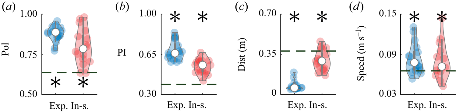
Figure 3. Predictive power of the proposed model for four metrics of collective behaviour: (a) polarization; (b) pursuit index (PI); (c) average inter-individual distance; and (d) average speed of the centre of mass. Circles represent individual trials for real (Exp.) or in silico (In-s.) experiments. Thick grey bars indicate first and third quartiles; thin grey bars identify minimum and maximum values; and white circles are the median. Dashed lines show chance levels; a star identifies a significant difference from chance in  $t$-test comparison at a significance level of 0.05.
Overall, Figure 3 points to a strong tendency of live fish to school in an in-line pattern, which is accurately captured through in silico experiments. Further insight can be garnered through the analysis of the eigenvalues of  $A_{\text {in-line},22}$ in (13), which was derived from linearization of the proposed model. Specifically, we used the calibrated values of
  $r_0$,
  $v_0$ and
  $\eta$ from Figure 2 to analyse the stability of in-line swimming with respect to
  $k_p$,
  $k_v$ and
  $d$ in Figure 4. Numerical computation of the eigenvalues confirmed the theoretical proposition from the Routh–Hurwitz criterion that small values of
  $d$ hinder stability. For sufficiently large values of
  $d$, there was a wide range of combinations of the gains that exhibited stability. Using calibrated values of
  $k_p$ and
  $k_v$, we always attained stability for any choice of
  $d$ above approximately one BL, in agreement with observations on inter-individual distance in Figure 3. In contrast to the kinematic model of Reference Filella, Nadal, Sire, Kanso and EloyFilella et al. (Reference Filella, Nadal, Sire, Kanso and Eloy2018) that suggests a beneficial role of large values of
  $k_p$ and
  $k_v$, we discovered a richer scenario where large values of
  $k_p$ may destabilize the swimming pattern. A sample video of the effect of perturbations on in-line swimming is included as a supplementary movie.

Figure 4. Stability analysis of in-line swimming as a function of social and hydrodynamic interactions, in the form of heat maps of the maximum real part of the eigenvalues of  $A_{22}$ in (13) for: (a,b,c)
  $r_0 = 3.1 \ \mathrm {mm}$ and (d,e,f)
  $r_0=0 \ \mathrm {mm}$ (no hydrodynamic interactions). For each of the two scenarios, we consider three values of inter-individual distances
  $d$: (a,d) 0.5 BL; (b,e) 1 BL; and (c,f) 2 BL. Other simulation parameters are mean values from Figure 2:
  $\eta = 1.77 \ \mathrm {s}^{-1}$ and
  $v_0 = 0.094 \ \mathrm {m}\ \mathrm {s}^{-1}$. White regions identify stability boundaries and black points are mean values from Figure 2.
For completeness, in Figure 4, we also present the results obtained by setting  $r_0=0$, that is, dismissing hydrodynamic interactions without modifying any other model parameter. Hydrodynamic interaction effectively leads to a repulsion zone between animals swimming in-line that would otherwise not be present. Repulsion has been widely documented in the literature on mathematical models of animal groups, but generally attributed to a social response (Reference Vicsek and ZafeirisVicsek & Zafeiris, 2012), with the exception of Reference Gazzola, Hejazialhosseini and KoumoutsakosGazzola et al. (Reference Gazzola, Hejazialhosseini and Koumoutsakos2014) who also documented hydrodynamically-based repulsion. For a given value of
  $d$, we also registered a wider range of gain combinations that guaranteed stability; however, the extent of the difference became negligible for distances above one body length. Comparable insight can be gathered for A-dipoles, as presented in the supplementary material.
6. Conclusions
Here, we have presented and analysed a mathematical model of collective behaviour of zebrafish pairs. The model combines the jump persistent turning walker of Reference Mwaffo, Anderson, Butail and PorfiriMwaffo et al. (Reference Mwaffo, Anderson, Butail and Porfiri2015) with the interaction model by Reference Filella, Nadal, Sire, Kanso and EloyFilella et al. (Reference Filella, Nadal, Sire, Kanso and Eloy2018) toward a realistic description of zebrafish locomotion and of social and hydrodynamic interactions. The model consists of a system of coupled nonlinear stochastic differential equations for the speed and turn rate of each fish. Model parameters were calibrated using the real data on zebrafish pairs swimming in shallow water of Reference Zienkiewicz, Barton, Porfiri and Di BernardoZienkiewicz et al. (Reference Zienkiewicz, Barton, Porfiri and Di Bernardo2015a).
The calibrated model was successful in predicting all of the main features of the collective response of live animals. Not only did the animals exhibit strong shoaling and schooling tendencies, by swimming in close physical proximity and aligning their bodies, but they also opted for an in-line pattern where one fish would lead and the other would follow. A contribution of this study was to demonstrate local stability of this specific collective pattern through a detailed analysis of the linearized dynamics. Above a critical value of the inter-individual distance, in-line swimming becomes stable for a wide parameter range. This is in stark contrast with side-by-side swimming, which does not emerge as a viable solution of the model.
Taken in toto, these results question some of the assumptions that are often used in modelling fish behaviour (Reference Vicsek and ZafeirisVicsek & Zafeiris, 2012), which explains the mechanisms underlying schooling (Reference Partridge and PitcherPartridge & Pitcher, 1979; Reference WeihsWeihs, 1973) and draws inference of the leader–follower relationship from experimental observations of their orientation (Reference Krause, Hoare, Krause, Hemelrijk and RubensteinKrause et al., 2000). First, our theoretical results indicate that repulsion emerges from hydrodynamic interactions, rather than being a social rule pursued by individuals. Second, the long debate regarding the determinants of schooling patterns, with some fish occupying frontal positions and other rear ones, may reduce to a simple stability problem for the group. Neither reduced swimming costs nor foraging benefits are needed for fish pairs to opt for in-line swimming. Third, the inference of leadership traits from the frequency of instances in which an animal initiates a turn that is followed by others could be skewed by the stability of in-line swimming. Specifically, should the animals differ in their noise parameters, we would detect a false leader–follower association.
The main limitation of the model is that it neglects the reverse von Kármán wake generated by self-propelled swimmers, which results in a poor representation of the flow field immediately behind the dipole. The flows around the fore-body and to the sides of the dipole are, however, representative of those produced by a swimming fish. This is likely relevant in the study of in-line swimming, by adding further dynamics into the collective response (Reference Liao, Beal, Lauder and TriantafyllouLiao et al., 2003) and potentially mitigating the short-range decay of hydrodynamic interactions observed in the present model. While the vortex dipole model for fish swimming has been used in a variety of analytical models of swimming, there exists a need for explicit experimental validation.
There are several additional directions for the potential improvement of the model, which include: (i) the development of a dynamic model for the speed in the form of a stochastic different equation, similar to that of Reference Zienkiewicz, Barton, Porfiri and Di BernardoZienkiewicz et al. (Reference Zienkiewicz, Barton, Porfiri and Di Bernardo2015a,Reference Zienkiewicz, Barton, Porfiri and Di Bernardob) to overcome the approximation of constant speed and include additional mechanisms of social interaction; (ii) the extension to hydrodynamic interactions with walls in the tank and background water currents toward an improved understanding of the transition from in-line to side-by-side swimming as a function of the flow speed (Reference De Bie, Manes and KempDe Bie et al., 2020); and (iii) the extension of individual differences in the stability analysis that could help explain the modulatory role of fish body size on schooling and shoaling (Reference Karakaya, Macrì and PorfiriKarakaya et al., 2020; Reference ReebsReebs, 2001).
Acknowledgements
We are grateful to Dr E. Kanso for offering precious directions in the implementation of the finite-dipole model.
Funding Statement
This research was supported by the National Science Foundation (CMMI 1505832 and CMMI 1901697).
Declaration of Interests
The authors report no conflict of interest.
Author Contributions
Conceptualization, M.P and S.D.P.; methodology, M.P., M.K., R.R.S., and S.D.P.; software, M.P. and M.K.; validation, M.P., M.K., and S.D.P.; formal analysis, M.P.; investigation, M.P., M.K., R.R.S., and S.D.P.; data curation, M.K.; writing – original draft, M.P. and S.D.P.; writing – review and editing draft, M.P. and S.D.P.; visualization, M.K.; supervision, M.P. and S.D.P.; project administration, M.P.; funding acquisition, M.P. and S.D.P. All authors approved the final submitted draft.
Data Availability Statement
Replication data can be found as supplementary material at https://doi.org/10.1017/flo.2021.5.
Ethical Standards
Experiments analysed herein were originally approved by the University Animal Welfare Committee of New York University under protocol number 13-1424.
Supplementary Material
Tables of experimental trajectories of all zebrafish, a table of calibrated model parameters, and mathematical derivations and results for the case of A-dipoles have been provided with the submission. Supplementary material is available at https://doi.org/10.1017/flo.2021.5.


 Open access