


1 Introduction
Self-control is viewed in economics and other disciplines as a key individual characteristic responsible for effective self-regulation and personal goal attainment (Moffitt et al., Reference Moffitt, Arseneault, Belsky, Dickson, Hancox, Harrington, Houts, Poulton, Roberts, Ross, Sears, Murray Thomson and Caspi2011). Lack of self-control is thought to explain suboptimal choices and outcomes in many life domains, including financial decision making, health, and education. Given the importance of self-control, this individual trait is widely studied theoretically and empirically in many different fields (Duckworth et al., Reference Duckworth, Milkman and Laibson2018).
In the economics literature, researchers usually model problems of self-control through time-inconsistent preferences that predict choices such as planning to go on a diet starting next week but not going on the diet when next week arrives. Two well-known models that can capture such behaviours are the hyperbolic (Loewenstein & Prelec, Reference Loewenstein and Prelec1992) and quasi-hyperbolic (Laibson, Reference Laibson1997) discount models. The latter model has attractive analytical features that have contributed to its popularity in economics (Frederick et al., Reference Frederick, Loewenstein and O’Donoghue2002), and for this reason we focus on it in our paper. The underlying assumption of the model is that agents have a “present bias” toward current consumption, as the values of all future rewards are downweighed relative to rewards in the present (in addition to the standard exponential discounting of delayed rewards). Economists have applied quasi-hyperbolic discounting theoretically and empirically to explain problematic behaviours across a wide variety of domains such as financial decision making (Laibson et al., Reference Laibson, Repetto and Tobacman1998), health behaviours (DellaVigna & Malmendier, Reference DellaVigna and Malmendier2006; Gruber & Kőszegi, Reference Gruber and Köszegi2001; Schilbach, Reference Schilbach2019), and work effort (Augenblick et al., Reference Augenblick, Niederle and Sprenger2015; Kaur et al., Reference Kaur, Kremer and Mullainathan2015).
In stark contrast to these diverse domains of application, most experimental research aimed at quantifying present bias has focused on a single specific reward type, namely money, and on samples from developed countries, in particular students at research universities. Further, most studies have used a cross-sectional design, which is not a true test of time inconsistency (Halevy, Reference Halevy2015; Read et al., Reference Read, Frederick and Airoldi2012).Footnote 1 Only a longitudinal design permits a test of inconsistent planning, the key prediction of the quasi-hyperbolic model (O’Donoghue & Rabin, Reference O’Donoghue and Rabin1999). In this paper, we address each of these shortcomings that have characterised much of the existing literature. We next expand upon each of these points in turn.
In this paper, we estimate and compare time preferences for money, healthy foods, and unhealthy foods. We thus contribute to the literature by identifying the shape of time preferences for food rewards. While the quasi-hyperbolic model has been applied to explain behaviour across a variety of domains, several recent experimental studies find no present bias for money (Andersen et al., Reference Andersen, Harrison, Lau and Rutström2014; Andreoni & Sprenger, Reference Andreoni and Sprenger2012a; Andreoni et al., Reference Andreoni, Kuhn and Sprenger2015; Augenblick et al., Reference Augenblick, Niederle and Sprenger2015). An influential interpretation of these findings (Cohen et al., Reference Cohen, Ericson, Laibson and White2020) holds that experiments using money will fail to detect present bias if subjects engage in arbitrage: if subjects integrate experimental earnings with borrowing and savings opportunities outside the experiment, they will simply switch from sooner to later payment at the market interest rate, revealing linear utility and no present bias.
Clearly, to shed light on this issue it is necessary to compare present bias for monetary and non-monetary rewards. Augenblick et al. (Reference Augenblick, Niederle and Sprenger2015) compare present bias for money and real effort, finding present bias for effort but not money. In their experiment, choices over effort (which is aversive) may be interpreted as revealing preferences toward leisure (a reward) if it is assumed that time not spent working for the experimenters is instead devoted to the consumption of leisure. However, since it is only the effort choice that is elicited and controlled for in the experiment, it is possible that this effort instead displaces another aversive use of time—such as domestic work, study, or an outside form of market employment—as opposed to leisure. This, in effect, is the real effort analogue to the potential confound of arbitrage in experiments using money. While previous studies (discussed next) have compared impatience and risk preference for monetary and direct consumption rewards, ours is the first to do so for present bias.Footnote 2 For now, we point out that if present bias is real but confounded by arbitrage in experiments using money, then we would expect to find present bias for food but not money. We return to the issue of arbitrage in the discussion.
With regard to other economic preferences, it has been found that people tend to be less patient (as distinct from present biased) for primary rewards than for money (Estle et al., Reference Estle, Green, Myerson and Holt2007; Odum & Rainaud, Reference Odum and Rainaud2003; Reuben et al., Reference Reuben, Sapienza and Zingales2010; Tsukayama & Duckworth, Reference Tsukayama and Duckworth2010; Ubfal, Reference Ubfal2016) but that risk preferences estimated for money and food rewards are essentially the same (Levy & Glimcher, Reference Levy and Glimcher2012).Footnote 3 These contrasting results highlight the importance of studying the consistency of preferences across domains separately for each economic preference. Moreover, within the domain of foods, unhealthy foods may be more tempting, triggering more present bias. It is thus also important to compare time preferences between healthy and unhealthy food.
A key feature of this paper is our sample of 697 relatively poor adolescents in China. Most previous studies have focused on the so called WEIRD subject pool (Henrich et al., Reference Henrich, Heine and Norenzayan2010). WEIRD refers to samples drawn from populations that are Western, Educated, Industrialised, Rich and Democratic. One reason why carefully designed studies do not find present bias for money may simply be that the participants, having been admitted into top universities, did not have serious self-control problems to begin with.Footnote 4 Indeed, several recent studies provide evidence that participants from developing countries show present bias for money (Balakrishnan et al., Reference Balakrishnan, Haushofer and Jakiela2020; Banerji et al., Reference Banerji, Goto, Ishizaki, Kurosaki, Lal, Paul and Tsuda2018; Clot & Stanton, Reference Clot and Stanton2014; Giné et al., Reference Giné, Goldberg, Silverman and Yang2018; Janssens et al., Reference Janssens, Kramer and Swart2017). Aycinena et al., (Reference Aycinena, Blazsek, Rentschler and Sprenger2020) find impatience for money and a preference to smooth payments over time in a sample of low-income Guatemalans, but do not find present bias. There is also evidence that certain clinical populations (e.g. prescription drug program enrolees and diabetes patients) show present bias for money (Abaluck et al., Reference Abaluck, Gruber and Swanson2018; Mørkbak et al., Reference Mørkbak, Gyrd-Hansen and Kjær2017). Our paper contributes to the still relatively limited evidence on the time preferences of non-WEIRD samples.
Our subjects differ not only on each of the dimensions of the WEIRD samples, but also in their age. Self-control established early in life is critical to personal development, yet few studies to date have estimated time preferences in children and adolescents.Footnote 5 Research in psychology has shown that poor self-control in childhood is associated with a range of damaging behaviours, for example cigarette smoking. Moreover, children with greater self-control are significantly more likely to be from socioeconomically advantaged families (Moffitt et al., Reference Moffitt, Poulton and Caspi2013).
To identify present bias we conduct a longitudinal experiment in schools. Halevy (Reference Halevy2015) distinguishes three properties of standard preferences over temporal payments relative to a dated collection of such preferences. Stationarity implies that the ranking of two temporal payments at time t depends only on the difference between the two payments and their relative delay. The standard cross-sectional design is a test of this property. Time invariance implies that preferences are not a function of calendar time. Time consistency requires that the ranking of temporal payments does not change as the evaluation perspective changes from t to t’. Only a true longitudinal design can test for this property. Halevy (Reference Halevy2015) finds that people can be time inconsistent and have stationary preferences at the same time, implying that the results of a cross-sectional design may be misleading.
Finally, conducting our experiment in school allows us to avoid selection into the study as well as attrition from it. Further, with access to administrative data from schools, we test the ability of our experimental measures to predict field outcomes such as academic performance.
697 Chinese high-school students participated in a five-week, incentivised longitudinal experiment using a modified version of the Convex Time Budget design (Andreoni & Sprenger, Reference Andreoni and Sprenger2012a) to elicit individual preferences for three reward types: money, healthy food and unhealthy food. Subjects faced the same set of decisions, featuring the same reward amounts delivered on the same dates, at two points in time. In the first session, all choices involved rewards to be received at two dates in the future, while in the second session the sooner rewards were available today. Our design also incorporates a test of rationality in the form of violations of the Generalised Axiom of Revealed Preference (GARP). We conducted our experiment during regular class time and all 697 subjects completed both sessions, resulting in zero attrition.
We highlight several key findings. First, we provide the first estimates of present bias for consumption rewards. At the median, averaging over all trials, our subjects choose to receive 2% more food on the sooner payment date when the decision is made on that day than when it is made in advance. Our structural estimate of
 for a representative agent is 0.69 for healthy food and for unhealthy food it is 0.71 (both are significantly less than one, but not significantly different from one another). Food consumption is highly consequential for people’s health. Focusing on the amount consumed in the moment, a representative agent who has a healthy
 and who participates in our experiment every week would become overweight in 4 years.
In contrast to some recent literature, we also find strong present bias for money. At the median, subjects choose to receive 4% more money on the sooner payment date when the decision is made on that day than when it is made in advance. Our structural estimate of
 for a representative agent is 0.65 for money (also significantly less than one, as well as significantly different from our estimates for food).
Next, in contrast to previous findings in the domain of risk, we find differences in the curvature of utility between monetary and primary rewards. For money, we confirm recent findings in the time preference literature that instantaneous utility is at best only mildly concave (Abdellaoui et al., Reference Abdellaoui, Bleichrodt, L’Haridon and Paraschiv2013; Andreoni & Sprenger, Reference Andreoni and Sprenger2012a; Cheung, Reference Cheung2020). However, for both healthy and unhealthy foods we find strong evidence of concave utility (implying a preference to spread rewards evenly over time), more in line with conventional findings in the domain of risk.
At an individual level, we find significantly positive and moderate correlations between individual measures of present bias for all reward type pairs [
 , as well as between individual measures of impatience [
 . We find even stronger correlations for a measure of the preference to smooth consumption over time [
 .Footnote 6 Together, these findings imply that conventional choices over money are moderately predictive of choices for food.
Finally, we find that our experimental measures of time preferences for both monetary and dietary rewards are predictive of subjects’ field behaviours. Adolescents who make less patient choices for any reward type are more likely to drink alcohol and have lower grades. Moreover, those who are more present biased for money and healthy food are more likely to drink alcohol and have lower grades.
The paper proceeds as follows: Sect. 2 describes our experimental design, Sect. 3 explains our empirical approach, Sect. 4 presents the results, and Sect. 5 provides a discussion of our findings.
2 Experimental design
2.1 Subject pool
We collected data from 697 adolescents (331 girls; average age 16.1 years, standard deviation 0.15 years) from four public high schools in Guiyang City, China in February and March 2019. We randomly selected 16 classes in tenth and eleventh grades to participate in the study. The University of Sydney Human Research Ethics Committee and principals of each collaborating high school approved the study. Teachers of the participating classes permitted the experiments to be conducted in class during regular school hours. No students opted out, and all participating students and their parents gave informed consent. The experiment was conducted in Mandarin (see Online Appendix 1 for an English translation of the instructions).
2.2 Task
Our experimental task is an extension of the convex time budget (CTB) design of Andreoni and Sprenger (Reference Andreoni and Sprenger2012a), which allows us to estimate subjects’ utility and discounting parameters using data from a single task. To simplify this task, we implement a discrete version of the CTB based upon Andreoni et al. (Reference Andreoni, Kuhn and Sprenger2015).
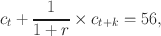
Following the CTB framework, we provide options that allocate amounts of a reward between two payment dates subject to a future-value budget constraint:

where
 denotes the amount of reward received at the sooner payment date
 ,
,
 denotes the amount of reward received at the later payment date
 , and
, and
 denotes the simple interest rate between the two dates. Between trials, we systematically vary the interest rate
 keeping the future value of the endowment fixed at 70. The back-end delay
 was always equal to three weeks.
Figure 1A shows a sample budget with an interest rate of 0%. In that case, regardless of which bundle a subject chooses, the amounts received on the two dates always sum to 70. To discretise this choice, we offer six evenly spaced options (shown as dots in Fig. 1A) along the budget line that a subject can choose from. There were always six options in every trial to keep choice difficulty constant. We exclude corner bundles [i.e.
 and
and
 ] from the choice set, as previous studies find that subjects who consistently choose corner bundles generate issues for structural estimation (Harrison et al., Reference Harrison, Lau and Rutström2013). Another advantage of this procedure is that by forcing subjects to receive payments on both dates, we equalise transaction costs without the use of a show-up fee.

Fig. 1 Experimental design. A: Budget constraint with 0% interest rate. The six dots on the budget line indicate bundles available to the chooser. B: Decision screen for the 0% interest rate trial. Each row represents one bundle. On the left is the amount received on the sooner date and on the right is the later date. Dots represent the quantity of a reward to be received on that date. The six bundles are presented in random order for each participant
Figure 1B shows the corresponding decision screen for the 0% interest rate trial. As well as stating the amounts of a reward that are available on each payment date, we also visualise these quantities to facilitate comparison of the alternatives. The order of presentation of the six options on the screen was randomised for each subject, and the subject chose their most preferred bundle by clicking on it.
The other simple interest rates we use are − 9%, 11%, 25%, 43%, 67% and 100% (see Fig. 2A for these seven budget sets). As the interest rate varies, a subject’s choices trace out a price expansion path in terms of sooner and later rewards, with the optimal choices depending upon both utility curvature and discounting parameters.
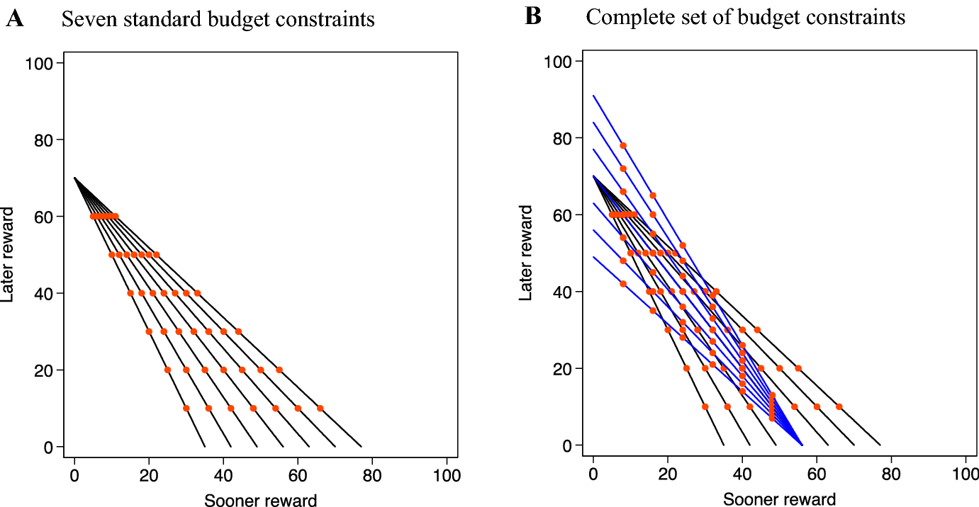
Fig. 2 Budget constraints
We further enrich this framework by adding an additional seven decisions to allow for a test of the consistency of subjects’ choices with the Generalised Axiom of Revealed Preference (Varian, Reference Varian1982), as recommended by Chakraborty et al. (Reference Chakraborty, Calford, Fenig and Halevy2017). We derive these additional choice sets from a present-value budget constraint:
and in these trials we vary the interest rate while holding the present value of the endowment fixed at 56. The interest rates
 for these additional trials are − 13%, 0%, 13%, 25%, 38%, 50%, and 63%. Figure 2B shows the complete set of budgets used in our design. The two sets of budget lines intersect one another, allowing us to count the number of times a subject’s choices violate GARP. The maximum number of GARP violations in this task is 91, while a random chooser would be expected to commit 12 violations. Note also that the trial with a 25% interest rate is presented twice (with other trials interleaved in between), allowing us to check for the consistency of subjects’ choices when making the same decision twice.Footnote 7
2.3 Timeline
Figure 3 shows the timeline of our five-week longitudinal experiment. In the first session in week one, subjects were presented with decisions where the sooner payment is in one week’s time (hence in week two) and the later payment is in four weeks’ time (hence in week five). In the second session in week two, the same subjects made the same sets of decisions over bundles of rewards received in weeks two and five, where the sooner payment is now available today.Footnote 8 This longitudinal design identifies dynamic inconsistency by comparing initial allocations in week one (when all rewards are in the future) with subsequent allocations in week two (when the sooner reward is in the present). In each school, all sessions were conducted at the same time of day and on the same day of the week to keep other variables such as hunger constant; for logistical reasons, the timing of the sessions differed slightly between schools. Before making their decisions in week one, subjects were told that they would be making decisions again in week two, and that one out of all their decisions would be randomly selected at the end of session two to be realised for payment. In the third session which took place in week five, subjects did not make any decisions and only received rewards. The experiment dates were between 25 February and 29 March 2019. Over this period, there were no public holidays, school vacations or examinations.

Fig. 3 Timeline of the experiment
After completing their decisions, subjects filled out a questionnaire which included demographic characteristics (in the first session) as well as current hunger and fatigue level,Footnote 9 and appetite ratings (in both sessions); see Online Appendix 2 for an English translation of these questionnaires.
2.4 Reward types
To compare time preferences for monetary and food rewards, we use a within-subjects design. Each subject faced the same sets of choices for three different reward types: money, healthy food, and unhealthy food. Before making any choices in week one, we asked each subject to choose their preferred healthy food reward and preferred unhealthy reward from three alternatives in each category. We did this to cater for different tastes and hence ensure that all subjects made decisions for foods that they liked. For healthy food, the available options were pecans, raisins, and almonds. For unhealthy food, the options were Skittles, M&M’s, and Lays. We chose these food rewards based on a pre-experiment survey of students’ favourite snacks.
A single food item—one Skittle, one chip, one raisin, etc.—counted as one unit of the good. For example, in a 0% interest trial, subjects may choose between 40 Skittles in one week and 30 Skittles in four weeks, 20 Skittles in one week and 50 Skittles in four weeks, and so on. For money, the budget was halved such that one unit of money equated to RMB 0.5 to equalise the value of different reward types.
To summarise, in a given session each subject made 14 decisions for each of three reward types, with all 42 decisions repeated in two separate sessions. The order of rewards was either healthy-money-unhealthy or unhealthy-money-healthy. This order was randomly selected for each subject in the first session, and then held constant for the second session. Thus, choices over the two food rewards were always separated by choices over money. The experimental interface was programmed using Qualtrics.
2.5 Payment
At the end of the second session, one decision of each subject (from either the first or second session) was randomly selected as the one that would count for payment. If this was a money trial, the payments were made in cash. If it was a food trial, the subject received the amounts of food they had chosen. Sooner payments (both money and food) were delivered one hour after the second session. In week five, research assistants returned to the schools at the same time as in week two to deliver the later payments. To protect privacy, regardless of reward type, we used non-transparent zip-lock bags to pack subjects’ payments. Therefore, monetary and food rewards were delivered to subjects in the same way.
Since we conducted the experiment during regular class hours in schools, the transaction costs to participate and receive payments are equalised throughout the study. Moreover, since subjects need to come to school anyway, we did not pay any additional show-up fee, and their compensation from the study was solely based on the choices that they made. Participants indicated a high level of trust in the experimental procedures, on average 5 on a scale from 1 (don’t trust at all) to 7 (no doubt at all).
3 Empirical approach
We next outline two approaches we adopt to measure subjects’ time preferences and utility curvature. Our first approach is to use descriptive measures of time preference and preference for smoothness that are based on simple proportions of rewards allocated to sooner versus later payment dates. These descriptive measures provide evidence on the behaviours we are interested in without needing to commit to specific structural assumptions. However, since descriptive measures cannot always cleanly distinguish between parameters, our second approach is to impose a quasi-hyperbolic discounted utility model (Laibson, Reference Laibson1997) and jointly estimate three parameters: the discount factor
 , present bias
 , and utility curvature
 . We find that these two approaches yield broadly consistent results.
3.1 Descriptive measures
3.1.1 Impatience
To investigate subjects’ impatience, without confounding it with present bias, we consider decisions made in the first session (week one) which result in bundles of rewards received in weeks two and five. Since all rewards are received in the future, present bias does not play any role. Subjects who select a bundle with a larger proportion of rewards allocated to the sooner payment date (week two) relative to the later date (week five) can be classified as more impatient (equivalently less patient).
Let
 be the amount of a reward that a subject would receive in week i based on a decision made in week j. We define impatience for each of the 14 week one decisions (
 ) for a given reward type as the proportion of the reward allocated to week two relative to the total amount of rewards in the chosen bundle, when the choice is made in week one:
Then, for each reward type separately, to measure an individual’s impatience we take the average of
 for that reward type over all 14 decisionsFootnote 10:

By construction, this measure is bounded between zero (most patient) and one (most impatient), although in practice because we removed corner bundles from the choice sets the measure cannot go all the way to these limits in our design.
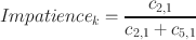
3.1.2 Present bias
Present bias occurs when an individual allocates a larger proportion of a reward to the sooner date when the sooner payment is immediate relative to when it is delayed, other things equal. To construct a descriptive measure of present bias, we first compare an individual decision made in week two when the sooner payment is today to the same decision made in week one when the sooner payment is delayed. We thus define present bias for a given decision scenario (
 ) as the difference in the proportion of the reward allocated to week two when making a choice in week two compared to when making the same choice in week one:

Then, for each reward type separately, to measure an individual’s present bias we take the average of
 for that reward type over all 14 decision scenarios:

By construction, this measure is bounded between negative one (most future biased) and one (most present biased). Again, because we removed corner bundles from our choice sets, the measure does not go all the way to these limits in our design.
3.1.3 Preference for smoothness
In addition to their time preferences, a subject’s choices in the experiment depend on the strength of their preference to smooth payoffs over time, as captured by the curvature of the utility function in a discounted utility model. A subject who has highly concave utility for a reward will have a strong preference for more mixed (temporally balanced) bundles, while one who has near-linear utility will tend to choose more extreme bundles near the corners of the budget set. To construct a descriptive measure of preference for smoothness, for a given decision trial (
 ), we calculate the difference between the sum of the amounts of a reward allocated to both dates and the absolute difference in those amounts, normalised by the sum of the amounts:

where
 represents the amount of a reward allocated to the sooner date and
 represents the amount of a reward allocated to the later date.
In the limiting case of a corner solution (where one of the
 s is zero), the numerator collapses to zero and so
 goes to zero. At the opposite extreme of perfect smoothing (such that
 ), it is the absolute difference term that collapses to zero and so
 goes to one.
Then, for each reward type separately, to measure an individual’s preference for smoothness we take the average of
 for that reward type over all 28 decision scenariosFootnote 11:

By construction, this measure is bounded between zero (no preference for smoothing) and one (maximum preference for smoothing), although in practice it does not go to these limits because we removed the corner bundles in our design.
3.2 Structural model
To conduct a parametric estimation of the discount factor, present bias, and utility curvature we assume a
 utility function and quasi-hyperbolic discount function (Laibson, Reference Laibson1997; O’Donoghue & Rabin, Reference O’Donoghue and Rabin1999). The instantaneous utility from experimental payments,
 , is:
, is:

The parameter
 is
is
 utility curvature, where
 indicates linear utility, and
 (
(
 ) indicates concave (convex) utility. With a quasi-hyperbolic discount function, the intertemporal utility from experimental payments
 received at date
 , and
, and
 received at date
 , is:
, is:

The parameter
 captures present bias. When
 , the discount function is exponential and there is no present bias, while
 indicates present bias. The variable
 is an indicator of whether the sooner payment date,
 , is immediate. The parameter
 is the weekly discount factor.
Given the discrete nature of the choice sets in our design, we estimate this model using multinomial logit (MNL) regression (Cheung, Reference Cheung2015; Harrison et al., Reference Harrison, Lau and Rutström2013) which compares the discounted utility of a subject’s chosen bundle to that of each of the available alternatives. Conditional on candidate values of the parameters being estimated, we use Eqs. (1) and (2) to compute the discounted utility of each of the six alternative bundles. Then, given the bundle chosen by the subject, the multinomial logit probability of the observed choice is given by:

where
 represents the utility of the chosen bundle,
 is a “noise” parameter, and
 represents the utilities of the six bundles in each trial. The estimates of
 and
and
 are chosen to maximise the log-likelihood of the observed choices, with standard errors clustered at the level of the subject.
We report representative agent models for each reward type, estimated in STATA using both the MNL procedure as well as the nonlinear least squares (NLS) estimation technique used by Andreoni and Sprenger (Reference Andreoni and Sprenger2012a) for continuous CTB data. Unless noted, our conclusions are qualitatively the same using either estimation procedure. In addition, we report the summary statistics of individual-level MNL models estimated in MATLAB for each subject and reward type. For individuals with extreme choice patterns exhibiting little variance, individual estimation is unreliable. Since we set bounds on the individual estimates for each parameter, this problem expresses itself as one or more parameter estimates running to the bounds.Footnote 12 Despite this issue, we report results using individual estimates for all subjects, for two important reasons. First, this ensures consistency with our reporting of results using individual descriptive measures. Second, it allows us to evaluate the in- and out-of-sample prediction performance of our estimates under worst-case conditions. This confirms that even where our individual point estimates are not reasonable, they are nonetheless in line with our subjects’ behaviour. As a result, these boundary estimates do not adversely affect our ability to correctly predict subjects’ choices in Sect. 4.3 below (see Online Appendix 5 for details).
4 Results
We present the results in four parts. We first establish that subjects’ choices are consistent and rational. We then analyse their time preferences (impatience and present bias) and utility curvature using both descriptive measures and structural estimates as defined in the previous section. Next, we explore the correlation between time preferences for monetary and food rewards. We conduct both in- and out-of-sample prediction analyses to examine to what extent choices for money predict choices for food and vice versa. Finally, we study the relationship between our experimental measures of time preferences and field behaviours: BMI, smoking, alcohol consumption, and academic performance.
4.1 Consistency of subjects’ choices with GARP
Table 1 shows the average number of GARP violations and Afriat’s critical cost efficiency index (Afriat, Reference Afriat1967) separately for the three reward types and two sessions. For a given reward type and session, the maximum number of possible GARP violations in our design is 91. On average, subjects made 1.72 GARP violations for money, 1.71 for healthy food, and 1.84 for unhealthy food. The number of violations did not significantly differ between any of the reward types or within a reward type between sessions. For all reward types, the Afriat index is 0.98. Although this is significantly less than 1 (
 ), it is close to 1 indicating that our subjects were highly rational. Moreover, their scores are higher than in previous studies with comparable age groups. Harbaugh et al. (Reference Harbaugh, Krause and Berry2001) found Afriat’s index to be around 0.95 for children aged between 7 and 11 years, and around 0.94 for undergraduates, both lower than in our study; their experiment design also involved discretised budget sets. Overall, we conclude that our subjects behaved in a highly rational manner allowing meaningful analysis of their preferences.Footnote 13
Table 1 Average number of GARP violations and Afriat’s index for different reward types in each session

|
Average no. of GARP violations |
Afriat’s index |
||
|---|---|---|---|
|
1st session |
Money |
1.68 |
0.98 |
|
Healthy |
1.65 |
0.98 |
|
|
Unhealthy |
1.78 |
0.98 |
|
|
2nd session |
Money |
1.75 |
0.98 |
|
Healthy |
1.77 |
0.98 |
|
|
Unhealthy |
1.90 |
0.98 |
|
4.2 Time preferences
When presenting our results for impatience, present bias and preference for smoothness, we proceed in the following order: we first present the descriptive measures for that preference, followed by structural estimates for a representative agent, and finally, the individual-level structural estimates.
4.2.1 Impatience
In Fig. 4, we plot the mean of
 from choices made in session one as a function of the interest rate.Footnote 14 As the interest rate increases, subjects choose to receive less on the sooner date, consistent with the law of demand. Figure 4 suggests that subjects were less patient for food than for money. At the median, averaging over all interest rates, subjects chose to receive 39% of their rewards on the sooner payment date for money, and 41% for healthy and unhealthy food (detailed data in Table 2). Wilcoxon signed-ranks test show that the differences in
 between money and healthy food, and between money and unhealthy food, are both significant (
 , see Table 3), but that the difference between healthy and unhealthy food is not significant (
 ). Our finding that subjects tend to be less patient for primary rewards than for money is consistent with previous studies (Estle et al., Reference Estle, Green, Myerson and Holt2007; Odum & Rainaud, Reference Odum and Rainaud2003; Odum et al., Reference Odum, Baumann and Rimington2006; Reuben et al., Reference Reuben, Sapienza and Zingales2010; Tsukayama & Duckworth, Reference Tsukayama and Duckworth2010; Ubfal, Reference Ubfal2016).

Fig. 4 Impatience for different reward types at different interest rates, based on choices in the first session. Dots (squares, crosses) represent the proportion allocated to the sooner reward in the first session for money (healthy food, unhealthy food). Long-dashed (short-dashed, solid) curves are the mean
 predictions using individual MNL estimates for money (healthy food, unhealthy food)
Table 2 Summary statistics of individual descriptive measures of impatience, present bias and preference for smoothness, by reward type

|
10th |
25th |
50th |
75th |
90th |
||
|---|---|---|---|---|---|---|
|
Impatience |
Money |
0.20 |
0.28 |
0.39 |
0.48 |
0.53 |
|
Healthy |
0.19 |
0.28 |
0.41 |
0.49 |
0.54 |
|
|
Unhealthy |
0.22 |
0.29 |
0.41 |
0.48 |
0.54 |
|
|
Present bias |
Money |
− 0.14 |
− 0.03 |
0.04 |
0.17 |
0.34 |
|
Healthy |
− 0.15 |
− 0.04 |
0.02 |
0.13 |
0.28 |
|
|
Unhealthy |
− 0.15 |
− 0.04 |
0.02 |
0.12 |
0.30 |
|
|
Preference for smoothness |
Money |
0.30 |
0.40 |
0.57 |
0.71 |
0.82 |
|
Healthy |
0.32 |
0.44 |
0.60 |
0.75 |
0.86 |
|
|
Unhealthy |
0.31 |
0.44 |
0.61 |
0.76 |
0.86 |
|
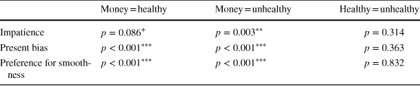
Table 3 Wilcoxon signed-ranks tests of differences in impatience, present bias and preference for smoothness between reward types
|
Money = healthy |
Money = unhealthy |
Healthy = unhealthy |
|
|---|---|---|---|
|
Impatience |
|
|
|
|
Present bias |
|
|
|
|
Preference for smoothness |
|
|
|


+ p < 0.1, *p < 0.05, **p < 0.01, ***p < 0.001
Turning to our MNL structural estimates for a representative agent (Table 4, top panel), we find that
 for all three reward types (
 which implies a negative discount rate. To understand this surprising finding, call a bundle back (front) loaded if in that bundle, a larger proportion of the reward is delivered at the later (sooner) date. In trials with a front-end delay (such that
 is not implicated in choices) and an interest rate of zero, a negative discount rate would express itself through subjects selecting back-loaded bundles.Footnote 15 Indeed, in zero-interest trials our subjects on average allocate 53.5% to the later date for money and 54% to the later date for healthy and unhealthy food, slightly more than an equal split of 50%. This behaviour is consistent with our estimate of
 .Footnote 16 Nonetheless, only 10.33% of our subjects choose the most back-loaded bundle for money (10.47% for healthy food and 9.76% for unhealthy food).Footnote 17
Table 4 Structural estimation results (standard errors in parentheses) using multinomial logit regression (MNL) and non-linear least squares regression (NLS) without background consumption

|
Money |
Healthy |
Unhealthy |
||
|---|---|---|---|---|
|
MNL |
|
− 0.0330 (0.0797) |
0.3160 (0.0850) |
0.2983 (0.0857) |
|
|
0.6574 (0.0356) |
0.6959 (0.0459) |
0.7161 (0.0425) |
|
|
|
1.0809 (0.0142) |
1.1198 (0.0234) |
1.1142 (0.0212) |
|
|
noise |
27.9009 (8.4884) |
11.2921 (3.6022) |
11.5058 (3.5440) |
|
|
NLS |
|
0.5994 (0.0211) |
0.7072 (0.0258) |
0.7202 (0.0280) |
|
|
0.8456 (0.0157) |
0.8852 (0.0183) |
0.8820 (0.0180) |
|
|
|
1.0338 (0.0053) |
1.0350 (0.0061) |
1.0408 (0.0061) |


Finally, Table 5 shows summary statistics of individual MNL estimates of
 for the three reward types. We find that for around 75% of subjects the point estimate of
 is greater than 1. The median of
 for money and unhealthy food is 1.01, and for healthy food it is 1.00. In Table 6, Wilcoxon signed-ranks tests indicate no significant differences in
 between any two reward types.
Table 5 Summary statistics of individual MNL structural estimates of
 , by reward type

|
10th |
25th |
50th |
75th |
90th |
||
|---|---|---|---|---|---|---|
|
|
Money |
− 0.50 |
0.01 |
0.58 |
1.84 |
4.91 |
|
Healthy |
− 0.41 |
0.08 |
0.91 |
2.34 |
5.27 |
|
|
Unhealthy |
− 0.42 |
0.04 |
0.88 |
2.52 |
5.39 |
|
|
|
Money |
0.05 |
0.34 |
0.79 |
1.15 |
5.45 |
|
Healthy |
0.05 |
0.32 |
0.87 |
1.23 |
8.43 |
|
|
Unhealthy |
0.05 |
0.39 |
0.91 |
1.45 |
10.07 |
|
|
|
Money |
0.83 |
0.95 |
1.01 |
1.25 |
2.33 |
|
Healthy |
0.82 |
0.93 |
1.00 |
1.24 |
2.57 |
|
|
Unhealthy |
0.79 |
0.94 |
1.01 |
1.28 |
2.86 |
|


Table 6 Wilcoxon signed-ranks tests of differences in the distributions of
 across reward types

|
Money = healthy |
Money = unhealthy |
Healthy = unhealthy |
|
|---|---|---|---|
|
|
|
|
|
|
|
|
|
|
|
|
|
|
|


+ p < 0.1, *p < 0.05, **p < 0.01, ***p < 0.001
4.2.2 Present bias
In Fig. 5, we plot the proportion of the reward allocated to the sooner date against the interest rate, separately for each reward and session. Dots (squares) represent the proportion allocated to the sooner reward in the first (second) session and the solid (dashed) curve represents the predicted aggregate choice behaviour implied by our structural
 model in the first (second) session when we estimate reward-specific parameters of that model by MNL at an individual level and predict the choices that maximise each subject’s utility in each trial.Footnote 18 The difference between allocations in the two sessions represents present bias. The more time consistent subjects are, the closer the solid and dashed curves will be. The fact that the dashed curve is above the solid one for all three reward types indicates that our subjects choose to receive more on the sooner date when the sooner date is today compared to when it is in the future, with the distance between the curves indicating the strength of present bias.

Fig. 5 Present bias for different reward types. Dots (squares) represent the proportion allocated to the sooner reward in week one (two) session. Solid (dashed) curves are the mean
 predictions using individual MNL estimates for week one (two) session. The difference between allocations in the week one and two sessions represents present bias
Our descriptive measures (Table 2 and Fig. 5) indicate that present bias is strongest for money. The median of our descriptive measure of present bias for money is 0.04. That is, averaging over all trials, at the median subjects allocate 4% more money to the sooner date in the second session. The median for healthy and unhealthy food is 0.02. Using Wilcoxon signed-ranks test we confirm a stronger present bias for money than for each dietary reward (
 ), and no significant difference in present bias between healthy and unhealthy food (
 ) (Table 3).
Turning to our MNL structural estimates for a representative agent (Table 4, top panel), we find economically and statistically significant present bias for all rewards, consistent with our descriptive analysis. For money we find
 (std. err. = 0.0356,
 ), for healthy food
 (std. err = 0.0459,
 , and for unhealthy food
 (std. err = 0.0425,
 ). In line with our descriptive measures,
 is smallest (present bias is strongest) for money.
Finally in our individual MNL estimates (Table 5), we find present bias (
 for around 65% of subjects, depending on the reward type. The median of
 for money is 0.79, smaller than for healthy food (0.87) and unhealthy food (0.91). These results are directionally consistent with both the descriptive measures and structural estimates for a representative agent. Wilcoxon signed-ranks tests show that individual structural estimates of
 differ significantly between money and unhealthy food and marginally for healthy and unhealthy food (Table 6).
Our finding of significant present bias for money differs from recent studies, including Andreoni and Sprenger (Reference Andreoni and Sprenger2012a), Andreoni et al. (Reference Andreoni, Kuhn and Sprenger2015), Andersen et al. (Reference Andersen, Harrison, Lau and Rutström2014) and Augenblick et al. (Reference Augenblick, Niederle and Sprenger2015) who all conclude that there is no present bias for money. In the discussion, we compare our design (study takes place at school during school hours) and subject pool (adolescents from a relatively poor background) with these studies and discuss potential reasons for this difference.
We also find present bias for consumption goods which is a novel contribution of our study. Augenblick et al. (Reference Augenblick, Niederle and Sprenger2015) estimate present bias for real effort, finding an aggregate estimate of
 . Our estimates thus indicate stronger present bias for food than for real effort.
4.2.3 Preference for smoothness/utility curvature
We find a stronger preference for smoothness for food rewards than for money. The median of our descriptive measure of preference for smoothness is around 0.60 for food and for money it is 0.57. A higher score for food indicates a stronger preference for more mixed bundles, and thus more concave utility for food rewards than for money. While the difference between money and food is highly significant (
 , Tables 2, 3), we do not find any difference in the preference for smoothness between healthy and unhealthy food.
Our MNL structural estimates for a representative agent (Table 4, top panel) are consistent with the descriptive analysis. The estimated utility curvature for money is not significantly different from zero, consistent with findings in Andreoni and Sprenger (Reference Andreoni and Sprenger2012a), Abdellaoui et al. (Reference Abdellaoui, Bleichrodt, L’Haridon and Paraschiv2013), Andreoni et al. (Reference Andreoni, Kuhn and Sprenger2015), Augenblick et al. (Reference Augenblick, Niederle and Sprenger2015) and Cheung (Reference Cheung2020). For both healthy and unhealthy food, we estimate significantly concave utility, indicating that our subjects have a preference to smooth food rewards over time.Footnote 19
Finally, our individual MNL estimates are also consistent with these conclusions. Table 5 shows that the median
 for money is 0.58, and for food between 0.88 and 0.91. Given the CRRA functional form, this indicates more concave utility for food than for money. In line with the comparison using descriptive measures, individual estimates of
 differ significantly between money and food (
 , Wilcoxon signed-ranks tests) but not between healthy and unhealthy food (Table 6).
4.3 Relationship between time preferences for money and food rewards
In summary, we have seen that subjects have different preferences for monetary and for food rewards. They are less patient, less present-biased, and have more concave utility for food than for money. In contrast, we find little systematic evidence of differences in any of these preferences between the two food reward types.
In this subsection we first use our descriptive measures to examine the extent to which time preferences for money and food are correlated within each individual. Using Spearman rank-order correlation analysis and descriptive measures of impatience, we find significantly positive, moderate correlations around 0.61 between individual impatience for all reward-type pairs (Fig. 6 panel A). This means that individuals who made less patient choices for money also made less patient choices for food, and those who made less patient choices for unhealthy food also made less patient choices for healthy food. Panel B of Fig. 6 illustrates the correlations between individual descriptive measures of present bias for different reward types. They are also significant and moderate at around 0.60. Preference for smoothness is a proxy for utility curvature. As shown in Fig. 6 Panel C, the correlation between any two reward types is significant and strong (around 0.
 .
.

Fig. 6 Correlations of individual descriptive measures of impatience, present bias and preference for smoothness across reward types. The line is the best linear fit
We next investigate to what extent individual MNL structural estimates for one reward type predict choices for the others. Since most studies in experimental economics rely on monetary incentives, it is important to understand the validity of extrapolating from such studies to different reward domains. We answer this question in two steps. First, we validate our structural estimation in sample. In other words, we ask to what extent our individual MNL estimates for a given reward type predict choices for the same individual and reward type. We then use this as a benchmark to assess out-of-sample prediction in the second step.
In Fig. 7A, B, first row, we plot the observed choice distributions in the first and second sessions, separately for each reward type. Bundles 1 to 6 are indexed according to their relative position along the budget line, with 1 being the most front-loaded and 6 the most back-loaded bundle within any given choice set. We see that in the first session, the choice distribution is similar for the two food rewards, with bundle 3 being the modal choice. For monetary rewards, the modal choice is bundle 6 which allocates most to the later date, consistent with the finding that subjects are more patient for money than for food. In the second session, owing to present bias, the tendency to choose bundles 1 and 2 (allocating most to the sooner date) increases for all reward types. We also see that bundles 1 and 6 are less frequently chosen for food than for money, consistent with the finding that subjects have a stronger preference to smooth food rewards over time.

Fig. 7 In-sample prediction. Bars illustrate the proportion of choices of each bundle type (1 is the most front-loaded bundle and 6 is the most back-loaded). The first row shows the observed choice distributions. The second row shows the in-sample predicted choice distributions
To examine how well our structural estimates explain an individual’s choices for the same reward type (in-sample prediction), we calculate the utility of each bundle in each trial using each individual’s reward-specific MNL estimates, and predict that the individual will choose the bundle with the highest utility in each trial. As illustrated in the second row of Fig. 7A, B, this predicts the general tendency to pick each bundle type quite well, although a Chi-squared test indicates that there is a significant difference between the observed and in-sample predicted choices

In Table 7, entries along the diagonal show the percentage of choices correctly predicted using the in-sample estimates. Across all three reward types, we correctly predict 57% of individual choices in both the first and second sessions.Footnote 20 This is our benchmark to compare the ability of estimates based on choices over money to predict choices over food.
Table 7 The percentage of correct predictions using individual MNL estimates of row type to predict choices of column type

|
Money (%) |
Healthy (%) |
Unhealthy (%) |
|
|---|---|---|---|
|
Money |
57.7 |
44.6 |
45.1 |
|
Healthy |
46.7 |
56.9 |
46.3 |
|
Unhealthy |
45.6 |
44.7 |
56.4 |
Random choice at best can predict 16.5% of choices
For out-of-sample prediction, we can use individual MNL estimates for money to calculate the utility of each bundle in each food trial and predict that an individual will select the bundle with the highest utility. This procedure amounts to predicting the same choice in each food trial as predicted for the corresponding money trial, as summarised in the bottom left panel in Fig. 7A, B. We now correctly predict 45% of choices for food. Chi-squared tests confirm that the performance is indeed significantly worse when we use estimates from choices over money to predict choices over food (
 , Table 8).Footnote 21
Table 8 Chi-squared tests for out-of-sample prediction performance

|
|
|
|
|---|---|---|
|
|
|
|


 Prediction performance using estimates for money to predict choices on healthy food or unhealthy food.
 Prediction performance using estimates for healthy food to predict choices on healthy food.
 Prediction performance using estimates for unhealthy food to predict choices on unhealthy food
+p < 0.1, *p < 0.05, **p < 0.01, ***p < 0.001
4.4 Experimental measures and field behaviours
In this section, we assess the predictive power of our descriptive measures of impatience and present bias to explain smoking, alcohol consumption, body mass index (BMI), and academic performance. Information on smoking and alcohol consumption was collected through self-reports from all 697 adolescents. BMI and grades for the three core units (Chinese, Mathematics, and English) were obtained from the administrative records of the participating high schools.
Figure 8 summarises our data on BMI and academic performance. 59% of our subjects have BMI in the normal range (
 ), while 28% are underweight and 13% are overweight (mean BMI = 21.21, 75th percentile = 22.04, std. dev. = 4.88). Academic performance in China is assessed on a scale from 0 to 100; we combine the grades in the three core units by averaging them. The average combined grade for a student in our sample is 55.7% (std. dev = 9.79) and the highest is 79.2%, indicating medium to low academic performance in our sample. Very few subjects (7.17%) reported smoking cigarettes and 13.63% reported drinking alcohol.
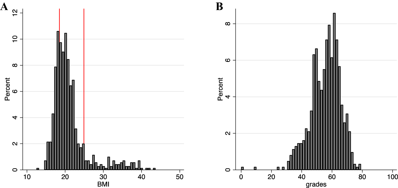
Fig. 8 Summary statistics for field behaviours. A: Histogram of BMI, calculated by dividing weight (in kilograms) by height (in metres) squared, obtained from schools’ administrative data. The area between the red vertical lines indicates the healthy range of BMI (18.5 to 24.9). B Histogram of academic performance (the average score for Chinese, Mathematics and English), obtained from schools’ administrative data
To establish if there is any relationship between time preferences and field behaviour, we run twelve regressions. In each regression, one of the four field behaviours (dependent variable) is regressed on one of three pairs of standardised domain specific descriptive measures for impatience and present bias, controlling for subjects’ age, gender, self-reported wealth, hunger, fatigue, and trust in the experimenter. We use linear regression for continuous outcome variables (BMI and academic performance); for binary outcome variables (smoking and alcohol consumption) we use logit regression and report marginal effects. Table 9 summarises the effects of the domain specific preference measures; full results including the control variables are in Online Appendix 7. For example, all else being equal, a one standard deviation increase in impatience (present bias) toward money is associated with an 4.57% (4.44%) increase in the likelihood of consuming alcohol.
Table 9 Relationship between impatience and present bias (standardised as z score), and field behaviours

|
Money |
Healthy |
Unhealthy |
|
|---|---|---|---|
|
BMI |
|||
|
Impatience z score |
− 0.5184* (0.2210) |
− 0.0883 (0.2167) |
− 0.3851 + (0.2028) |
|
Present bias z score |
− 0.2351 (0.1972) |
− 0.3980* (0.1861) |
− 0.2724 (0.2099) |
|
Smoking |
|||
|
Impatience z score |
0.0089 (0.0114) |
0.0017 (0.0118) |
0.0108 (0.0113) |
|
Present bias z score |
0.0218* (0.0094) |
0.0033 (0.0095) |
0.0101 (0.0098) |
|
Alcohol |
|||
|
Impatience z score |
0.0457** (0.0140) |
0.0362* (0.0143) |
0.0442** (0.0138) |
|
Present bias z score |
0.0444** (0.0139) |
0.0278* (0.0133) |
0.0187 (0.0130) |
|
Grades |
|||
|
Impatience z score |
− 1.2549** (0.4092) |
− 0.8833* (0.4257) |
− 1.1656** (0.3922) |
|
Present bias z score |
− 1.2560** (0.4111) |
− 1.0612* (0.4294) |
− 0.9527* (0.4135) |
|
N |
697 |
697 |
697 |
The table presents results of twelve regressions. In each regression, one of the field behaviours (dependent variable) is regressed on the standardised impatience and present bias measured in one domain. Unreported control variables are: age, gender, wealth, hunger, fatigue, and trust in the experimenters. BMI and Grades (the average grade for the three core units: Chinese, Mathematics and English) are continuous variables obtained from the administrative records of the participating high schools. Smoking and Alcohol are binary variables collected through self-reports from all subjects. BMI and Grades results are from OLS regressions. Smoking and Alcohol results are from Logit regressions and the marginal effects are reported. Standard errors clustered on individual subjects are in parentheses
+ p < 0.1, *p < 0.05, **p < 0.01, ***p < 0.001
The most prominent associations we find are between the domain-specific time preferences and grades. Adolescents who made less patient choices and showed stronger present bias for money, healthy food or unhealthy food had lower grades. Moreover, adolescents who were less patient and more present-biased for money and healthy food were more likely to drink alcohol. For alcohol and unhealthy food, we see the same effect of impatience, but the effect of present bias is smaller and not significant. Very few adolescents in our sample report smoking, which is likely why we only find one significant effect: subjects who were more present biased for money were more likely to smoke. The relationship between time preferences and BMI may be counter-intuitive: subjects who were less patient for money and unhealthy food and subjects who were less present biased for healthy food had lower BMI, but the effect is only at margin.
To summarise, our measures of patience and present bias have strong associations with alcohol consumption and academic performance. Time preferences for money and for food predict almost the same set of field behaviours equally well. We explore the implications of these findings in the discussion.
5 Discussion
The model of present-biased time preferences is one of the cornerstones of behavioural economics. In this paper, we provide evidence that fills some major gaps in empirical research on this model. Using data from an incentivised, within-subjects, longitudinal experiment in Chinese high schools, we estimate and compare present-bias, patience, and utility curvature for three types of rewards: money, healthy food, and unhealthy food. While researchers have applied the quasi-hyperbolic discount model to explain sub-optimal decision-making in a wide variety of domains, to date empirical evidence of present bias parameters has come predominantly from experiments using money, with many recent studies finding no present bias for money (Andersen et al., Reference Andersen, Harrison, Lau and Rutström2014; Andreoni & Sprenger, Reference Andreoni and Sprenger2012a; Andreoni et al., Reference Andreoni, Kuhn and Sprenger2015; Augenblick et al., Reference Augenblick, Niederle and Sprenger2015). This raises the possibility that either present bias is not the right behavioural model, or that it is not a feature of the samples and/or rewards used in these studies. While several studies (such as those conducted in developing countries) address the diversity of the sample, ours is the first to provide estimates of present bias for consumption rewards.
We find strong present bias for food rewards. Our conjecture that unhealthy food might be more tempting and thus trigger more present bias is not supported by the results. At the median, subjects in our experiment allocate on average 2% more food to the sooner date when that date is today rather than in the future. This is the same for both healthy and unhealthy food. Structural estimates yield a present-bias parameter of 0.69 for healthy food and 0.71 for unhealthy food (not significantly different between the two).
To give an indication of the consequences of such preferences, we calculated the caloric intake of a representative agent assuming they take part in the same experiment every week and compared it to the caloric intake of a time-consistent chooser (focusing on how much is chosen for consumption in the moment as opposed to total consumption from the experiment). Compared to time-consistent choosers, our representative agent would consume around 246 more calories each week from the experiment alone, resulting in 1.6 kg increase in weight per year. Holding all else constant, an average high-school student with
 would become overweight in 4 years. This estimate should be regarded as a lower bound, as it does not incorporate other dietary choices that subjects make that may also involve temptation. In line with this intuition, Vadeboncoeur et al. (Reference Vadeboncoeur, Townsend and Foster2015) found that university students can gain up to 4 kg in their first year of study, which coincides with the time in life when they start to take responsibility for their own nutrition.
Our finding of present bias for dietary rewards is a novel contribution to the literature. Nonetheless, a potential concern that arises over the use of food as rewards is satiation. We argue that the characteristics of our sample make this less of a concern. Our subjects are of low-to-medium socioeconomic status, and most have low to normal BMI, implying that they are unlikely to be satiated for all reward types used in our experiment. Indeed, for trials with a negative interest rate, the modal choice was the most front-loaded bundle that also contained the largest total amount of a food, implying that our participants prefer more food to less.
Several prominent recent studies do not find present bias for monetary rewards. It is thus notable that we use the same rigorous preference elicitation methods but find present bias for money. As mentioned in the introduction, an influential interpretation of the absence of present bias for money is in terms of arbitrage. Under this hypothesis, subjects in a money discounting experiment will simply choose sooner payment in trials that offer less than the market interest rate, and later payment at higher interest rates. They will thereby reveal a discount rate equal to the market interest rate, linear utility, and no present bias.
Several aspects of our results are inconsistent with the arbitrage hypothesis. First, arbitrage predicts the choice of the most front-loaded bundle at a zero-interest rate in both sessions. Instead, in the first session our subjects choose mixed bundles at zero interest even for money. We estimate
 , implying a negative discount rate, for both the representative agent and around 75% of individuals. Our subjects thus display a clear regard for future monetary rewards even in the absence of market interest, and our estimate of their discount factor is not simply revealing a market interest rate. Second, the preference for smoothing that we observe in the choice of a mixed bundle at zero interest (in the first session) is also inconsistent with arbitrage, and is observed for all three reward types. Finally, since the market interest rate is orthogonal to the presence or absence of a front-end delay in the experiment, arbitrage cannot explain the shift toward more front-loaded bundles in the second session (Fig. 7A, B, top-left panels), resulting in our estimate of
 for money.
Of course, subjects cannot engage in arbitrage if they lack access to market opportunities for borrowing and saving. For students in the age group that we study, it is likely they would have access to the market for saving, but not borrowing. In that case, participation in our experiment represents a rare opportunity to engage in borrowing, sometimes at a zero or even negative interest rate, which can be exploited by choosing a front-loaded allocation and then saving at a higher interest rate outside the experiment. Once again, this is inconsistent with our finding of patient choices at zero interest in the first session, resulting in an estimate of
 for money.
Why then do we observe present bias for money where several previous studies did not? These contrasting findings may be due to differences in the subject pool as well as the procedures of the experiment. Instead of university students, our sample consists of Chinese adolescents of low-to-medium socioeconomic status. Our finding of present bias for money in this sample is consistent with the findings of most previous studies that were conducted in developing country settings.Footnote 22 With regard to experimental protocols, we conducted our experiment at schools during regular school hours, whereas subjects in most laboratory studies had to take the initiative to sign up for the experiment and come to the lab on time. We argue that this may generate selection bias, as subjects who are able to show up to a previously scheduled experiment on time are likely to have good self-control. This selection bias will of course be compounded if the subjects are recruited from the students at a research university, who have already exhibited self-control sufficient to place them at a top school.
Our findings regarding the curvature of utility are notable in light of recent controversy over the nature of utility in choice over time (Abdellaoui et al., Reference Abdellaoui, Bleichrodt, L’Haridon and Paraschiv2013; Andreoni & Sprenger, Reference Andreoni and Sprenger2012a; Cheung, Reference Cheung2020). These recent studies find that instantaneous utility for money in choice over time is far less concave than Bernoulli utility (also over money) in choice under risk, a finding that stands in sharp contrast to the long tradition in theory that assumes concave utility, and the strong psychological (Kahneman & Tversky, Reference Kahneman and Tversky1979) and biological foundations of S-shaped utility functions (Rayo & Becker, Reference Rayo and Becker2007; Robson & Whitehead, Reference Robson and Whitehead2020; Tymula & Glimcher, Reference Tymula and Glimcher2020; Woodford, Reference Woodford2012). We complement these recent findings by further demonstrating that instantaneous utility for money is also less concave than it is for consumption rewards. This further underscores the importance of studying different reward domains rather than drawing strong inferences from the study of a single domain alone, namely money.
An important question in behavioural economics is to what extent can we extrapolate findings from studies involving monetary rewards to other domains of decision making. In our experiment, we use an identical method to elicit preferences of each subject for three reward types, allowing for a meaningful within-subject comparison of estimates across rewards. We find that the strength of correlation varies with the preference under consideration. For impatience, the correlations between money and food are moderate, consistent with Reuben et al. (Reference Reuben, Sapienza and Zingales2010), whereas for present bias the correlations (while significant) are weaker. We find strong correlation in utility curvature for money and food, consistent with Levy and Glimcher (Reference Levy and Glimcher2011). This last result is striking given that we also find a sharp divergence in the magnitude of the curvature parameter between money and foods.
Our finding that preferences are generally correlated across reward types is consistent with the existence of a common valuation mechanism in decision making. Indeed, neuroeconomic studies that measured brain function during valuation have concluded that food and money rewards recruit the same neural substrates to encode value and there are no unique activated areas as a function of reinforcer type (Chib et al., Reference Chib, Rangel, Shimojo and O’Doherty2009; Kim et al., Reference Kim, Shimojo and O’Doherty2011; Valentin & O’Doherty, Reference Valentin and O’Doherty2009). The same brain regions are also involved in valuation of aversive outcomes (electric shocks) (Delgado et al., Reference Delgado, Jou and Phelps2011) and erotic stimuli (Sescousse et al., Reference Sescousse, Redouté and Dreher2010). Our work extends this earlier work, by showing that while each of the preferences we study is correlated across reward types, present-bias is less correlated than risk attitudes and patience. Therefore, researchers should be more cautious in extrapolating (individual-level) present bias for money to other domains than in doing so for the other preferences.
Our data allow us to relate elicited preference measures to field behaviours including self-reported smoking and alcohol consumption, as well as BMI and academic performance obtained from schools’ administrative records. We find that subjects who are less patient and more present biased for money and food are more likely to drink alcohol and have lower grades, leading to an overall less favourable health and economic outlook compared to subjects who are more patient and less present biased. Similar findings have been found by Sutter et al. (Reference Sutter, Kocher, Daniela and Trautmann2013).
Finally, while we have framed our paper in the language of the quasi-hyperbolic discount model, we note that our findings are also compatible with other hyperbolic discounting models and may thus be interpreted as evidence of time-inconsistent preferences more generally.Footnote 23
Acknowledgements
We thank Marco Castillo, Gretchen Chapman, Keith Marzilli Ericson, Paul Glimcher, Joseph Kable, Daniel Read, Bram de Rock, and Anya Samek for valuable discussions, as well as participants in the Sydney Workshop on Experimental Economics and Theory, 2019 TIBER Symposium on Psychology and Economics, 2019 IAREP/SABE conference on Economic Psychology and Behavioural Economics, 2019 European Meeting of the Economic Science Association and 2019 Annual Meeting of the Society for Neuroeconomics. Cheung acknowledges support from the Australian Research Council, Grant Number: DP170102818. Tymula acknowledges support from the Australian Research Council, Grant Number: DE150101032. Wang acknowledges PhD fellowship support from the Australian Research Council Centre of Excellence for Children and Families over the Life Course (CE140100027, CE200100025). We are grateful to the principals and teaching staff at the participating high schools for making this project possible.
Funding
Open Access funding enabled and organized by CAUL and its Member Institutions.
Data availability
The replication material for the study is available at https://osf.io/6rygs/?view_only=6ca960ae2c8d4ec0a7be4cece073d002 (https://doi.org/10.17605/OSF.IO/6RYGS).
Declarations
Conflict of interest
The authors have no conflict of interest to declare.


 β-δ
β-δ


 α,βandδ
 α,βandδ
 β-δ
β-δ


 Open access