


1 Introduction
Revenue management (e.g., Phillips, Reference Phillips2005; Talluri & Ryzin, Reference Talluri and van Ryzin2004) can be characterized as a set of propositions for rational retailers of how to sell the right inventory to the right consumer at the right time and the right price (Kimes, Reference Kimes1989). This is mostly achieved by allocation of inventory, by dynamic pricing of the good, or by some combination of both. Subsumed under this very general characterization are multiple models that differ from one another on one or more critical assumptions about the type of consumers who enter the market (e.g., myopic, strategic), the nature of the competition between the retailers (if there are more than one), the information structure (e.g., whether price information is common knowledge among the retailers), the nature of the demand (stochastic vs. deterministic, time-sensitive), capacity constraints, replenishment of the good during the selling season, salvage costs, and, in general, the rules that govern trade in the market. A major contribution of the theoretical literature in revenue management has been the demonstration of how important these assumptions are and what effect they might have on inventory allocation and dynamic pricing. A major contribution of the experimental literature, mostly in economics and marketing, has been to demonstrate systematic deviations of traders’ decisions from the theoretical models.
In the present paper, we contribute to both theory and experimentation by introducing and subsequently testing a stylized model of dynamic pricing under retailer competition. Specifically, competition in our model is conducted through the retailers making alternating offers to consumers. Our approach builds on previous studies by Mantin et al. (Reference Mantin, Granot and Granot2007) (MGG), and Mak et al. (Reference Mak, Rapoport and Gisches2012) (MRG), which also extends a line of experimental research on monopolistic dynamic pricing that includes Rapoport et al. (Reference Rapoport, Erev and Zwick1995) and Mak et al. (Reference Mak, Rapoport, Gisches and Han2014).
In the family of models investigated in MGG and MRG as well as here, the consumer's valuation of the good is denoted by v. The two retailers do not know the value of v, but they are assumed to have common prior knowledge about the probability density of v. The two retailers are assumed to maximize their individual payoffs (profits) over a season (horizon) with a finite number of periods, and in each period they can post independently, and with no restrictions, new prices. In each period, the consumer is free to visit one and only one of the two retail stores. A critical element of this family of models concerns the pattern of visits: if in a period the consumer visits a retailer and observes a posted price that exceeds their valuation, then, in the next period, they may either return to the same retailer with probability P or switch to the competing retailer with probability 1 − P. MGG refer to the special case of P = 0, where the consumer deterministically switches retailers from one period to another, as “zigzag competition.”
There may be several alternative reasons for this first-order Markov store-choice pattern of visits by the consumer in such finite, multi-period, dynamic pricing settings. As noted in the marketing literature on brand choice and brand loyalty, switching behavior may be attributed to variety seeking (Lillien et al., Reference Lilien, Kotler and Moorthy1992; Kahn, Reference Kahn1995), as the consumer is assumed to have no prior knowledge about the posted prices in the market at any given period. The consumer switching probability 1 − P may serve as a proxy to the consumer's loyalty, or reflect their geographical proximity to the two stores that may change from one period to another. It also may reflect the consumer's experience at the store, the type of service they encounter, the actual time that elapses from one period to another, and their shopping habits.
MGG considered the case of myopic consumers, who purchase the good if and only if its valuation is higher than the posted price, and then extended their original model to strategic (i.e., forward looking) consumers. MRG considered the latter case in more detail. MGG extended their model of a single consumer to a model with multiple consumers, whose valuations are privately known and independently and identically distributed according to a uniform distribution. Importantly for our study, both MGG and MRG have noted that, under zigzag competition, the setting for multiple consumers trivially coincides with that of one consumer; a major purpose of our study is to test this conclusion experimentally. As discussed in detail below, our experiment showed that the theoretical invariance with respect to the number of consumers did not hold.
The present paper makes two major contributions. The first contribution is an extension of the finite-horizon dynamic pricing models of MGG and MRG to a model where the horizon is indefinite with probabilistic continuation. This is equivalent to an infinite horizon with time discounting in which all players, including retailers and consumers, have the same per period time discount factor for payoffs (see, e.g., Roth & Murnighan, Reference Roth and Murnighan1978; Zwick et al., Reference Zwick, Rapoport and Howard1992). The motivation of this extension is that for many goods, even so-called seasonal goods, the assumption that the “world ends” precisely after a finite number of periods is frequently made to gain mathematical tractability rather than reflect reality. The finite-horizon assumption might be appropriate for products with which the selling firm only has a limited number of opportunities to change prices during the selling season, such as fresh food that needs to be sold within a day. On the other hand, in cases where the selling season is long with numerous opportunities to change price dynamically, the infinite-horizon approach might be more appropriate.
In terms of experimental research on dynamic pricing, the extension to an infinite horizon seems to create a problem as experimental sessions terminate at finite time. While, strictly speaking, infinite-horizon models with time discounting are not experimentally testable, the way around this problem is to adopt an indefinite horizon approach and setting the continuation probability (i.e., the size of the discount factor) sufficiently low so that the probability of inordinately long sessions becomes negligible. Therefore, in the present study, we implemented the following procedure. If the consumer rejects an offer in a period, and therefore they are still “active” in the market, then the selling season continues with continuation probability δ or ends due to a random process with termination probability 1-δ, and the active consumer earns zero.
The second contribution is a change of focus in the present paper from one consumer to multiple consumers; a major purpose of the present study is to experimentally test the effects of the number of consumers on the pricing of the (homogenous) good and, consequently, on the evolution of this market. We proceed under the specification, in keeping with MGG and MRG, that if there are multiple consumers in the market, then any consumer's valuation, v, is ex ante independently and identically distributed according to a uniform distribution. We also adopt the complete information specification that, as in MGG and MRG, the price history is commonly known. With these specifications, the equilibrium pricing and purchase decisions of the sellers and consumers should not be affected by the number of consumers. Such equivalence is essentially an equivalence between selling to one buyer with a prior valuation distribution (such as in some business-to-business settings) and selling to a market of multiple consumers with valuations that are independently and identically distributed according to the same distribution (such as for many fast-moving consumer goods). However, behaviorally, it is important to see whether and how human sellers’ pricing decisions, as well as human consumers’ purchase decisions in response to the prices, could differ according to the size of the market. There are several reasons why the descriptive power of the analytical prediction of equivalence is questionable:
First, some of the consumers may appear to be more myopic than others—they would be more likely to purchase whenever their valuation is higher than the currently offered price, and less likely to attempt to strategically wait for a prospectively lower price with higher earnings in future periods. Retailers who are aware of the presence of such heterogeneity in consumer strategic behavior might adjust their pricing decisions accordingly. The presence of myopic consumer decisions in dynamic pricing contexts is a well-known experimental finding. For example, in an experimental study on dynamic pricing, Mak et al. (Reference Mak, Rapoport, Gisches and Han2014) reported that a substantial percentage of their buyer subjects behaved myopically although they were not instructed to do so. Osadchiy and Bendoly (Reference Osadchiy and Bendoly2015) also reported that while many of their subjects exhibited strategic behavior, some were consistently purchasing myopically. Further theoretical and experimental developments include Baucells et al. (Reference Baucells, Osadchiy and Ovchinnikov2017), Kremer et al. (Reference Kremer, Mantin and Ovchinnikov2017), and Chen and Zhao (Reference Chen and Zhao2020), among others. In our case, if different numbers of consumers lead to differences in consumers’ tendency to be myopic or to attempt strategic waiting, the retailers might respond to such differences with different pricing strategies.
Second, the number of consumers can influence the length of the season. This is because the season ends when either a random termination event occurs, or the market clears. With a single consumer, the market clears immediately upon purchase, potentially cutting the season short even if a random termination wouldn’t have happened. This has implications for learning in terms of observations of ex post suboptimal decisions, i.e., decisions that are suboptimal vis a vis the ex post observations of the full set of posted prices by retailers in a season after the season is over. In the single-consumer case, the only observable ex post suboptimal decision is ex post “too late” (passing on a lower price and buying later at a higher price, or the season ending without a purchase despite encountering a price that is below valuation). In the multiple-consumer case, ex post “too early” purchases (buying at a higher price than the season's lowest that appears afterwards) become observable alongside ex post “too late” instances. This difference in ex post suboptimal observations might influence consumer behavior in the multiple-consumer case compared to the single-consumer case. Specifically, the ability to observe ex post “too early” purchases might lead to more strategic waiting behavior by consumers in the multiple-consumer case.
Lastly, since different consumers might purchase in different periods at different prices, there can be social comparison effects that are not present when there is only one consumer. These can be due to, for example, fairness concerns, as well as socially induced regret (over the possibility that another consumer might be able to purchase at a better price) and could affect consumer purchase decisions as well as the pricing decisions of retailers who anticipate such effects. However, since consumers’ valuations vary and are only privately known, horizontal comparison between consumers’ surplus is not possible. Even if another consumer purchases at a lower price than a focal consumer during the same season (most likely at a later period), there is no guarantee that the other consumer's surplus is higher than the focal consumer's, thus potentially reducing the impact of fairness considerations among consumers. The more pronounced comparison is likely to be the consumer's own ex post comparison of their decisions during a season against the prices in that season, which could induce regret vis-a-vis the realization of ex post suboptimality (as discussed in the previous paragraph).
This paper presents our theoretical and experimental research contributions. Section 2 formally states our model of zigzag competition as employed in our experiment. Our equilibrium analysis suggests that price offers decrease exponentially across periods over the season. Moreover, when there are multiple consumers in the game, as long as their valuations are ex ante independently and identically distributed, the equilibrium predictions are the same regardless of the number of consumers.
Section 3 describes our experiment, which was designed to test the implications of the model and account for the dynamics of play and behavioral deviations across multiple iterations or seasons of the stage game. In accordance with common experimental procedures, we simplified the game presented to the experimental subjects in two different ways. First, for all experimental conditions, we impose a deterministic switching pattern on all the consumers to create a zigzag competition setting. As a consequence, the subjects (retailers) in our experiment had a simpler task as they had to consider only one rather than two sources of uncertainty. Secondly, we have restricted the experimental investigation to a single (relatively high) value of the continuation probability (δ = 0.75). To investigate evolution of behavior from experience, we iterated the basic dynamic pricing game for multiple seasons, and had the valuations of each of the consumers drawn randomly and independently on each season. Player roles (i.e., Retailer 1, Retailer 2, Consumer) remained fixed across all seasons to minimize confusion due to constant changes of role and guarantee sufficient data for each player.
Section 4 reports the main findings of the experiment. Briefly, our experimental study showed that retailer subjects often overpriced relative to equilibrium predictions. In addition, the theoretical invariance with respect to the number of consumers was violated: consumers seemed to be more prone to strategic waiting in the first period of the season when there were multiple consumers (compared with when there was only one consumer), leading to a decrease in the per-consumer payoff of the retailer who made the price offer in the first period and a corresponding increase in per-consumer payoff of the other retailer. There is also evidence of within-session evolution that led to lower retailer prices that were closer to equilibrium predictions, and higher tendency for consumer strategic waiting, as the session progressed. Section 5 concludes by summarizing our results and outlining extensions of the model for future research.
2 The model
2.1 A dynamic pricing model
We model the selling season as a non-cooperative game among three players including two retailers called Retailer 1 and Retailer 2, and N Consumers. Over the duration of the game, which consists of an indefinite number of periods, each Consumer demands one unit of an indivisible good. Each Retailer has N units of the good, which is of zero value for them. Each Consumer's valuation of the good, which is denoted by v, is privately known by the Consumer but not by the Retailers. Rather, the two Retailers hold a common prior knowledge that v is independently and identically distributed among the Consumers following the uniform distribution over the interval [0, ῡ].
In period 1 all of the Consumers visit Retailer 1, who offers to sell them the good at the price p 1. Each Consumer independently and simultaneously decides either to accept the offer or reject it. If all Consumers accept the offer, then the season terminates, each Consumer earns v − p 1 (v being the Consumer's own valuation), Retailer 1 earns Np 1 (as the marginal cost of the good is zero for both Retailers), and Retailer 2 earns zero. If some Consumers, say n of them, accept the offer, but the remaining N − n Consumers reject the offer, then each accepting Consumer earns v − p 1 and leaves the game, Retailer 1 earns np 1, and Retailer 2 earns zero, while the season continues to the next period with continuation probability δ and terminates with probability 1 − δ.
Period 2—assuming that it takes place—is structured in the same way with the exception that Retailer 2 makes the price offer p 2. The game proceeds accordingly with the Consumers zigzagging between the two Retailers until last remaining Consumers in the game accept a price p t at period t or the season terminates with no trade, whichever comes first. In any period t:
(a) if t is odd, each Consumer who accepts the offer in that period earns a payoff of v − p t , Retailer 1 earn p t per accepting Consumer, and Retailer 2 earns 0;
(b) if t is even, each Consumer who accepts the offer in that period earns a payoff of v − p t , Retailer 1 earns 0, and Retailer 1 earn p t per accepting Consumer.
Every price offer is commonly known once it is posted to the Consumers. Put differently, each Retailer knows the entire history of the offers when it is their turn to post a price and how many Consumers are still active in the market. It is also commonly known that there is no scarcity: each Retailer holds at least N units of the good.
As mentioned in Sect. 1, this game is formally equivalent to the one in which the Consumers zigzag infinitely many times between the two Retailers and each of the three players has the same per period time discount factor for payoffs.
2.1.1 Equilibrium properties
We focus on pure-strategy rational expectations equilibria in which the Retailer's price offers are deterministic conditioned on the history of trade, regardless of whether that history is in or out of equilibrium. Proofs of the following results are relegated to Online Appendix 1.
Lemma 1
In any strategy pricing equilibrium, a Consumer with valuation v 1 does not buy later than a Consumer with valuation v 2, if v 1 > v 2.
Proposition 1
Let α be the unique solution in (0,1) of the equation δ 2 α 4 − 2α + 1 = 0. The dynamic pricing game has a unique pure-strategy pricing equilibrium, in which:
(1) the equilibrium price in period t is p t * = v t * r = ῡα t (1 − δ)/(1 − δα),
where r = [α(1 − δ)]/(1 − δα).
(2) a Consumer whose valuation is contained in the interval (v t+1 *, v t *) = (ῡα t , ῡα t−1) purchases the good in period t;
(3) a Consumer whose valuation is exactly ῡα t−1 purchases the good in period t or max{1, t − 1};
(4) the ex ante probability of a transaction happening in period t is δ t−1(v t * − v t+1 *)/ῡ.
=δ t−1 α t−1(1 − α);
(5) the ex ante payoff of Retailer i is ῡα (1 − α)(1 − δ) (δα 2) i−1/[(1 − δα)(1 − δ 2 α 4)];
(6) the ex ante payoff of the Consumer is ῡ(1 − α)2(1 + δα)/[2(1 − δα)(1 − δα 2)],
According to Proposition 1 (statement (1)), prices decay exponentially across periods, a feature that is shared with the monopolistic dynamic pricing model analyzed in Rapoport et al. (Reference Rapoport, Erev and Zwick1995). The Consumer's behavior and the posted prices exhibit “skimming” characteristics. The segment of the distribution of v that is skimmed decreases in size exponentially across the periods—by a factor of α from period to period—and so are the upper/lower bounds of the skimmed segment. The equilibrium price in any given period is always r times the upper bound of the posterior distribution of v in that period. Lastly, ῡ, which is the upper bound of the prior distribution for v, only appears as a scaling factor. All of these results hold because of the symmetry imparted by the random termination process (or, alternatively, because all the players in the dynamic pricing game have the same per period time discount factor and the game has infinitely many periods), as well as the fact that v is uniformly distributed with a lower bound of 0. Table 1 illustrates the equilibrium solution and the out-of-equilibrium properties (to be discussed next) for the parameter values implemented in our experiment, namely, δ = 0.75 and ῡ = 1000.
Table 1 Equilibrium solution and the out-of-equilibrium properties for the parameter values implemented in our experiment

|
Figure 1 exhibits values of α and r as a function of δ. On both curves, the points for δ = 0.75—the value used in our experiment—are marked. Figure 1 shows that the parameter α is not very sensitive to the value of δ; in fact, it always lies within the interval [0.5, 0.55] over the full possible range of δ. Recall that α is the ratio by which the equilibrium prices decrease from period to period, and also the ratio by which the support of the updated distribution of the Consumer's valuation is skimmed from period to period (see Proposition 1). Figure 1 therefore suggests that the equilibrium price always undergoes an approximately 50% discount per period, while the Consumer valuation range is at the same time skimmed by approximately 50%.
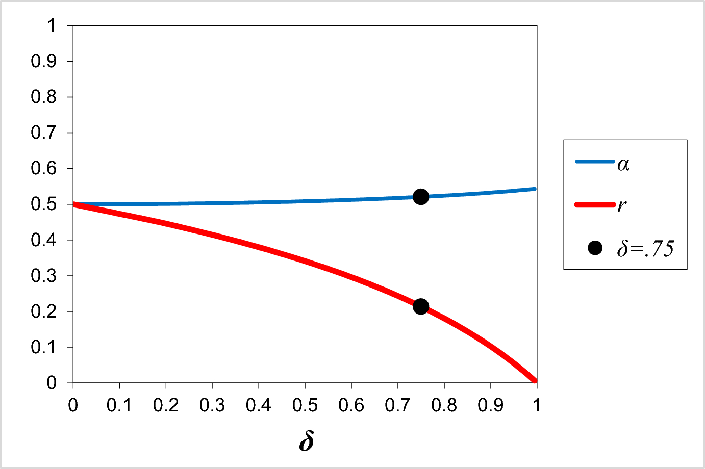
Fig. 1 Plots of the parameters α = v t+1 */v t * and r = p t */v t * as a function of the probability of continuation δ for the dynamic pricing game
On the other hand, Fig. 1 shows that r is relatively sensitive to δ. Recall that r is the ratio between the equilibrium price in a period and the high end of the valuation distribution in the same period; for example, it is the ratio of the period 1 equilibrium price relative to ῡ. Its steady decrease as δ increases, while α remains largely around 0.5, suggests that high discount factor leads to strong competition that drives down prices, while forward looking Consumers’ strategic waiting leaves the period-to-period skimming largely unaffected. As δ → 0+, then r tends to the single-period monopolistic selling limit of ½. As δ → 1−, r tends to the Coase conjecture limit of 0 (see e.g., Coase, Reference Coase1972; McAfee & Wiseman, Reference McAfee and Wiseman2007).
2.2 Out-of-equilibrium properties
The equilibrium solution for the model in Proposition 1 is obviously useful for data analysis if both the Retailers and the Consumer follow the equilibrium path on each period of the selling season. Clearly, it is unrealistic to expect them to do so. If they depart from the equilibrium path, then the expressions stated in the propositions are no longer valid. Best response predictions have to be derived for each of the models to account for the decision in period t + 1 conditional upon the posted (rather than predicted) price offers up to this period.
Consider a sequence of posted price offers up to period t and label them p 1, p 2, … p t . Then, generate the sequence v 1′, v 2′, … v t ′, v t+1′ as follows:
v 1′ = ῡ.
v s+1′ = min{(1 − δα)p s /(1 − δ), v s ′}.
It can be deduced from the proof of Proposition 1 (see Online Appendix 1) that the valuation of the best responding Consumer who accepts an offer in period s must be contained within [v s+1′, v s ′]. If a best responding Consumer's valuation is higher (lower) than the upper bound of this interval, then they accept (reject) the offer in period s. If their valuation is exactly the lower bound of this interval, then they may or may not accept the price offer; since this is a zero measure event, it is still legitimate to assume that the posterior distribution of the valuation v in period s + 1 is a uniform distribution on the interval [0, v s+1′]. This means that the posterior or updated distribution of v in any period which is in or out of equilibrium is, indeed, always a uniform distribution over a support with a lower bound zero.
The best response of a Retailer whose turn is to post an offer in period s, given the posterior distribution at that period, is given by p s ** = rv s ′, where r is computed from Proposition 1. Because all the offers are assumed to be known, any Retailer may work out the v s ′ in period s, given the previous history of play, whether that is in or out of equilibrium.
Finally, it is clear from the setup of the model and our derivations that, when there are multiple consumers in the game, as long as their valuations are ex ante independently and identically distributed, the equilibrium and out-of-equilibrium predictions are the same regardless of the number of consumers. Players’ strategies, including pricing, should also not be affected by how many Consumers there are (i.e., have not yet purchased) in the current period. This feature of our analysis was tested in the experiment reported in the next section.
3 Experimental method
3.1 Subjects
Two hundred and fifty-nine subjects participated in the experiment. The subjects were undergraduate students at the University of Arizona and the University of California, Riverside, who volunteered to take part in a group decision making experiment for payoff contingent on performance.
3.2 Design
The experiment had a three-condition between-subjects design. Subjects in all conditions played the dynamic pricing game described in Sect. 2 with different number of Consumers: one Consumer in Condition 1B, three Consumers in Condition 3B, and five Consumers in Condition 5B, respectively. Subjects participated in experimental session cohorts that, depending on the experimental condition, ranged from 12 to 15 in size. Within a session, they were randomly assigned to groups of three, five, or seven players according to whether the experimental condition was Condition 1B, 3B, or 5B for that session. Condition 1B included 24 groups of three players each (two Retailers, one Consumer) across all of its sessions; correspondingly, Group 3B included 15 groups of five players each (two Retailers, three Consumers); and Condition 5B included 16 groups of seven players each (two Retailers, five Consumers). In each of the three conditions, the game was iterated for 50 seasons.Footnote 1 Player roles (i.e., Retailer 1, Retailer 2, Consumer) were held fixed for every subject across all the seasons. However, the composition of each group was determined randomly by re-matching subjects in the same experimental session at the beginning of each season; these measures were implemented in order to minimize sequential effects over the seasons. Each experimental session consisted of two to five groups as detailed in Table 2. The valuation of each Consumer was drawn randomly and from the set {1, 2, … 1000} at the beginning of each season.
Table 2 Number of sessions and number of groups and subjects in each session in the respective conditions

|
3.3 Procedure
All the sessions were conducted in a large computer-controlled laboratory with networked terminals that were separated from one another by partitions. Communication between the subjects was strictly forbidden. Once they entered the laboratory, subjects were assigned randomly to their cubicles and proceeded to read the subject instructions at their own pace. The instructions for Condition 5B are presented in Online Appendix 2, where the terms Seller 1, Seller 2, and Buyer stand, respectively, for Retailer 1, Retailer 2, and Consumer in the model and the general terminology in this paper.
The instructions described the trading mechanism, explained the valuation of the good for the Consumer, and then informed the subject about the calculation of the payoff (profit) for each season, the probability of terminating each period randomly, the Retailer's computer screen, the Consumer's computer screen, and the determination of the final payoff for the session. All queries were answered privately by the experimenter.
Each period t was structured as follows. The Retailers were presented with their Decision Screen (see Online Appendix 2) that included information about the player role, period number, season number, and the pricing log of both Retailers’ prices in the season and how many active Consumers remain in the market. If t was odd (even), Retailer 1 (2) was instructed to post their price for the period.
The Consumer was presented with their Buyer Screen that displayed the Buyer's valuation of the good for the season, the period number t, the posted price for period t, the Buyer's potential payoff were they to accept the present offer (v t − p t ), and the pricing log (history) of both Retailers’ prices in the season.
At the end of each season, each group member was presented with a summary screen with information about all the posted prices in the season, the member's own transaction (if there was one), and the member's payoff for the season. Once all the groups in the session completed the season, the experiment proceeded to the next season. Thus, all the groups in a given session started each season at the same time.
At the end of the session, after completing 50 seasons, the total payoffs from m randomly selected seasons were converted to US dollars at a rate of 80 experimental profit points = $1.0 to become the subjects’ earnings, plus a $5 show-up fee which they received privately. The number m was the same across player roles in Condition 1B but varied between roles in Conditions 3B and 5B to mitigate disparity in dollar payments. Specifically, in Condition 1B, m = 10 for all roles; in Condition 3B, m = 5 for Retailer 1 and the Consumer while m = 20 for Retailer 2; in Condition 5B, m = 3 for Retailer 1, m = 12 for Retailer 2, and m = 5 for the Consumer; note that each subject was only informed about the m for the role they were assigned. Upon receiving payments, the subjects were dismissed from the laboratory. All the sessions were completed in less than two hours.
4 Results
Since subjects in the same experimental session were randomly re-matched from season to season during the session (while keeping to the same player role), the independent unit of data analysis should be the session. Hence, the means reported in this section, including those in the tables and figures, are all calculated with session as the unit of analysis unless otherwise stated. On the other hand, when performing statistical tests, we typically use regression (linear or logistic depending on whether the dependent variable is interval/ratio or binary) clustering variances by session subjects.Footnote 2 The same applies to testing deviation from equilibrium analysis benchmarks—we would typically create a dependent variable that is the difference between the experimental data point and the relevant equilibrium analysis benchmark, and then run an intercept-only regression model without covariates, again clustering variances by session subjects; statistically significant deviation from the benchmark can be tested by looking at whether the intercept term from such a regression analysis is significantly different from zero or not.
Less than 2% of the seasons ended with more than six periods (see Table 3). Hence, where a statistical analysis pertains to period-by-period variables such as the price in each period, we focus only on periods 1 to 6. Lastly, since there is evidence of within-session evolution (see below), we typically conduct statistical analysis with a distinction between whether a data point came from the earlier half of a session (Seasons 1 to 25) or the latter half (Seasons 26 to 50).
Table 3 Number of seasons of different lengths (number of periods)

|
Length (period) |
1 |
2 |
3 |
4 |
5 |
6 |
7–16 |
Total |
|---|---|---|---|---|---|---|---|---|
|
Condition 1B |
||||||||
|
Seasons 1–25 |
352 |
158 |
36 |
39 |
8 |
6 |
1 |
600 |
|
Seasons 26–50 |
384 |
140 |
36 |
21 |
11 |
2 |
6 |
600 |
|
Condition 3B |
||||||||
|
Seasons 1–25 |
143 |
114 |
54 |
34 |
15 |
5 |
10 |
375 |
|
Seasons 26–50 |
117 |
148 |
61 |
20 |
18 |
4 |
7 |
375 |
|
Condition 5B |
||||||||
|
Seasons 1–25 |
123 |
117 |
56 |
46 |
29 |
9 |
20 |
400 |
|
Seasons 26–50 |
119 |
122 |
89 |
35 |
21 |
4 |
8 |
398 |
In the next subsections, we first report basic results regarding the experimental decisions. We next report a set of analysis comparing the Retailer pricing and Consumer purchase decisions with best responses prescribed by equilibrium analysis. Afterwards, we report analysis that more directly relates to between-condition differences and within-session evolution.
4.1 Basic results
We first note that the average length of each season in the experiment, in terms of periods, is 1.66 for Condition 1B, 2.26 for Condition 3B, and 2.57 for Condition 5B (see also Table 3). These are all significantly different from each other at p < 0.01 by regression clustering variances by session.Footnote 3 The percentage of seasons that ended with transactions being made with all the Consumers is 74.25% (891 out of 1200) in Condition 1B, 47.2% (354 out of 750) in Condition 3B, and 42.86% (342 out of 798) in Condition 5B. The mean number of transactions per season is 0.74 (74% of the number of Consumers) for Condition 1B, 2.00 (67% of the number of Consumers) for Condition 3B, and 3.60 (72% of the number of Consumers) for Condition 5B.
Another basic result from the experiment is that Retailers often overpriced relative to equilibrium predictions (see, e.g., similar results in MRG and Rapoport et al., Reference Rapoport, Erev and Zwick1995). This is borne out in Fig. 2, which plots the mean prices by condition and earlier/latter half of the session; the equilibrium predictions are also plotted for comparison. Note that the mean prices did not always decrease as the period increases (a steady decrease would have conformed to a basic equilibrium prediction). Statistical tests show that the mean prices over periods 1 to 6 are often significantly different from equilibrium predictions at p < 0.05 according to intercept-only regression analysis clustering variances by subjects. The notable exceptions are the period 1 prices in the latter half of the session in Conditions 1B and 5B, suggesting within-session evolution that drove down prices towards the competitive equilibrium level.
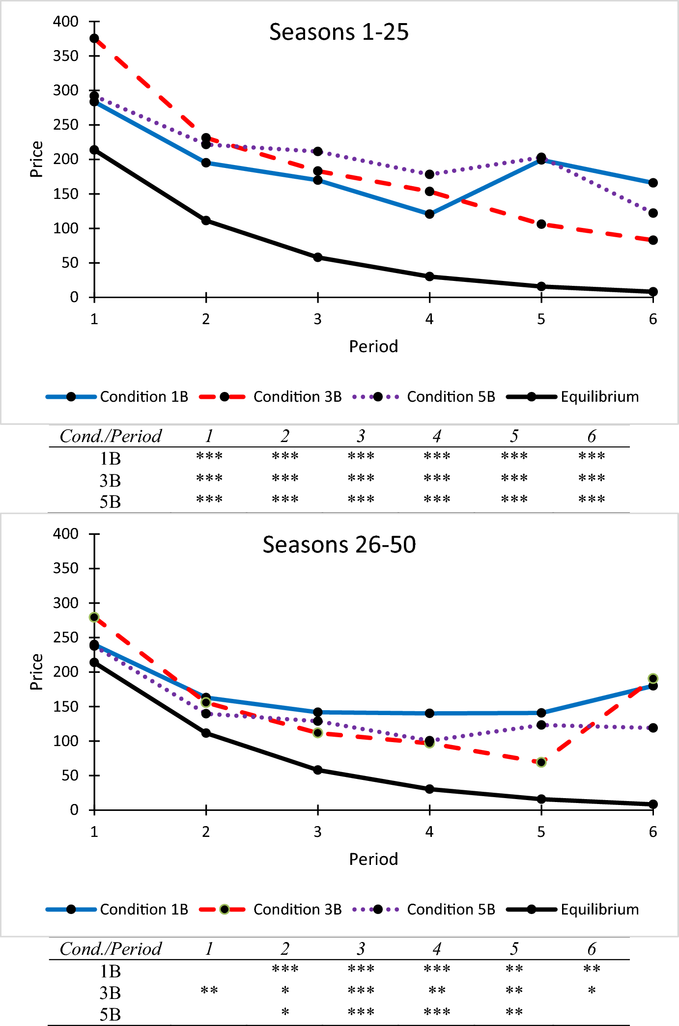
Fig. 2 Mean experimental and equilibrium prices up to period 6. The unit of analysis is the session. The accompanying tables indicate, with one or more asterisks, the mean prices by period that are significantly different from equilibrium prices according to an intercept-only regression analysis clustering variances by subjects (*p < 0.05, **p < 0.01, ***p < 0.001)
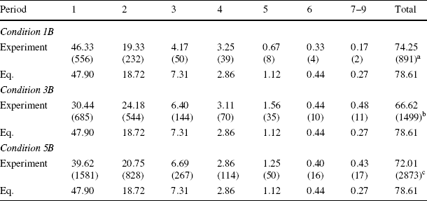
We next look at Consumer purchases. Define a Consumer journey as the sequence of price offers received and purchase decisions made during a season by a Consumer player; in Condition 1B, each season involved one Consumer journey, while in Condition 3B (5B), each season involved three (five) Consumer journeys. Table 4 displays the experimental and equilibrium percentages of Consumer journeys that resulted in purchases in periods 1–9. While equilibrium predictions suggest that transactions should occur in 78.6% of the Consumer journeys in the experiment over periods 1–10, the actual percentages in the experiment are markedly lower in Conditions 3B and 5B. In other words, the markets in the experiment cleared much less efficiently than suggested by theoretical analysis.
Table 4 Experimental and equilibrium percentages of Consumer journeys (see Sect. 4.1) by period of purchase (absolute frequencies in parentheses)
|
Period |
1 |
2 |
3 |
4 |
5 |
6 |
7–9 |
Total |
|---|---|---|---|---|---|---|---|---|
|
Condition 1B |
||||||||
|
Experiment |
46.33 (556) |
19.33 (232) |
4.17 (50) |
3.25 (39) |
0.67 (8) |
0.33 (4) |
0.17 (2) |
74.25 (891)a |
|
Eq. |
47.90 |
18.72 |
7.31 |
2.86 |
1.12 |
0.44 |
0.27 |
78.61 |
|
Condition 3B |
||||||||
|
Experiment |
30.44 (685) |
24.18 (544) |
6.40 (144) |
3.11 (70) |
1.56 (35) |
0.44 (10) |
0.48 (11) |
66.62 (1499)b |
|
Eq. |
47.90 |
18.72 |
7.31 |
2.86 |
1.12 |
0.44 |
0.27 |
78.61 |
|
Condition 5B |
||||||||
|
Experiment |
39.62 (1581) |
20.75 (828) |
6.69 (267) |
2.86 (114) |
1.25 (50) |
0.40 (16) |
0.43 (17) |
72.01 (2873)c |
|
Eq. |
47.90 |
18.72 |
7.31 |
2.86 |
1.12 |
0.44 |
0.27 |
78.61 |
Note that no transaction took place after period 9 in any condition in the experiment
aOut of a total count of 1200
bOut of a total count of 2250
cOut of a total count of 3990
To have an appreciation of the relative levels of strategic behavior among Consumers in the different conditions, for each Consumer player in each session, we look at instances when they were in the game (i.e. had not yet purchased in the current season) while their valuation was higher or equal to the current price; we then work out the percentage proportion of those instances throughout the session in which they did not buy, to form a measurement of attempted strategic waiting. We find that, across Consumer players in Condition 1B, the mean of this proportion is 33.00%, compared with 43.73% in Condition 3B and 41.08% in Condition 5B.Footnote 4 This suggests that Consumer players in the latter two conditions had a higher tendency to attempt strategic waiting by not making a purchase even when the current price was lower than their valuation.
Finally, the mean payoffs also suggest significant deviations from equilibrium predictions, as shown in Table 5. Note that, for more meaningful comparison between conditions, the payoff variables for the Retailers in Conditions 3B and 5B are normalized by the numbers of Consumers in those conditions (three and five, respectively). The table also indicates within-session evolution, which will be explored further in Sect. 4.3. With that in mind, we focus on the latter half of the session, in which Retailer 1 (Retailer 2) earned significantly less (more) than in equilibrium in Conditions 3B and 5B, but not 1B; the Consumer, meanwhile, earned significantly less than in equilibrium in Condition 3B in the latter half of the session, but not so in the other two conditions.
Table 5 Mean payoffs by condition and earlier/latter half of the session (s.d. in parentheses), together with the relevant equilibrium level

|
Condition 1B Seasons |
Condition 3B Seasons |
Condition 5B Seasons |
Eq. |
||||
|---|---|---|---|---|---|---|---|
|
1–25 |
26–50 |
1–25 |
26–50 |
1–25 |
26–50 |
||
|
Retailer 1 normalized |
92.83** (18.87) |
99.00 (23.44) |
110.98 (38.08) |
69.94*** (15.36) |
86.76* (30.71) |
72.52*** (30.41) |
106.83 |
|
Retailer 2 normalized |
36.48*** (15.16) |
26.05 (9.68) |
37.73*** (8.21) |
38.40*** (8.36) |
36.31*** (12.53) |
33.48*** (14.01) |
21.75 |
|
Consumer |
285.84*** (31.31) |
318.35 (17.76) |
219.76*** (38.98) |
290.50*** (44.04) |
277.92*** (55.67) |
316.75 (42.49) |
328.82 |
The unit of analysis is the session. Note that the Retailers’ mean payoffs are normalized by the number of Consumers in the experimental game in the corresponding condition, so that, for example, for Condition 3B and Retailer 1, the table shows the mean of the Retailer's payoff divided by three. Where the mean entry is significantly different from equilibrium according to an intercept-only regression analysis clustering variances by subjects, the entry is indicated by one or more asterisks (*p < 0.05; **p < 0.01; ***p < 0.001)
4.2 Analysis of deviations from best responses
To further understand these findings, we next report Fig. 3, which displays the mean deviations of Retailer prices relative to best response prescribed by equilibrium analysis. Note that, for period 1 pricing in the figure, we display the equilibrium price as the “best response”. Figure 3 shows that the Retailers largely overpriced with respect to best response in the earlier half of the session; however, as the session progressed, Retailers seemed to have been driven by competitive pressure to adhere more to equilibrium analysis prescriptions. This is especially the case with Retailer 2 in period 2 in response to Retailer 1's period 1 price.
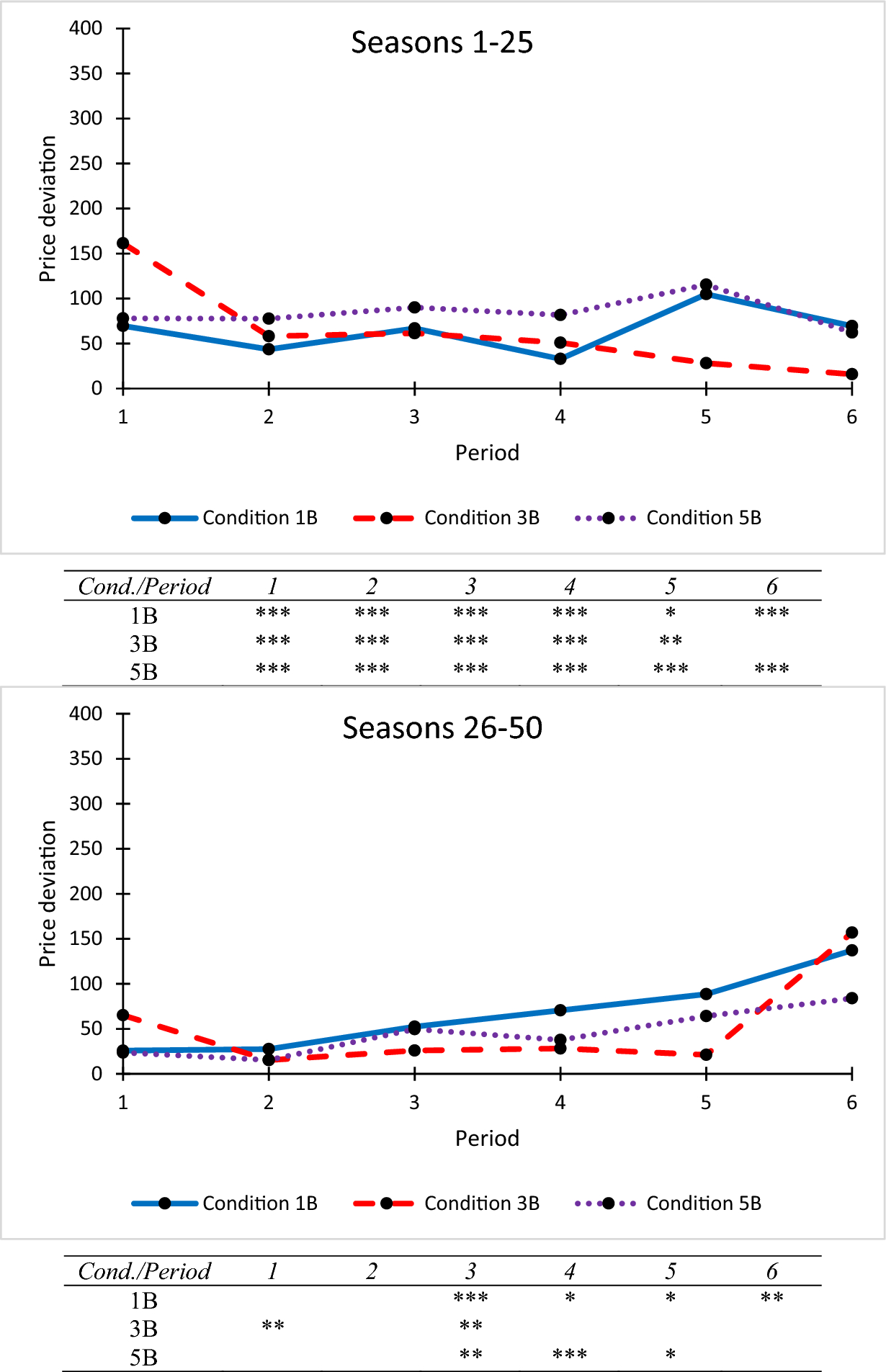
Fig. 3 Mean deviation of experimental prices from best response up to period 6. The unit of analysis is the session. The accompanying tables indicate, with one or more asterisks, the mean deviations by period that are significantly different from zero according to an intercept-only regression analysis clustering variances by subjects (*p < 0.05, **p < 0.01, ***p < 0.001)
We next compare the Consumers’ purchase decisions against best response based on equilibrium analysis derived from the equilibrium and out-of-equilibrium results in Table 1. Figure 4 displays the mean deviations of Consumer purchase decisions from best response. We code decisions such that a purchase decision is coded as 1 and a no-purchase decision is coded as 0, so that a purchase decision in the data when equilibrium analysis prescribes no purchase leads to a deviation of 1, while a no-purchase decision in the data when equilibrium analysis prescribes purchase leads to a deviation of − 1; if a decision in the data is the same what is prescribed by equilibrium analysis, the deviation is 0. Figure 4 shows that purchase decisions in period 1, compared with other periods, seem to adhere more to strategic benchmarks in the form of equilibrium analysis prescriptions, especially in the latter half of the session. But otherwise, Consumers often made purchases when equilibrium analysis suggested that they should not purchase. This type of behavior finds an analogy in previous research on sequential search behavior (e.g., Mak et al., Reference Mak, Seale, Rapoport and Gisches2019; Zwick et al., Reference Zwick, Rapoport, Lo and Muthukrishnan2003), where subjects often stopped to purchase when the optimal strategy was to continue searching.
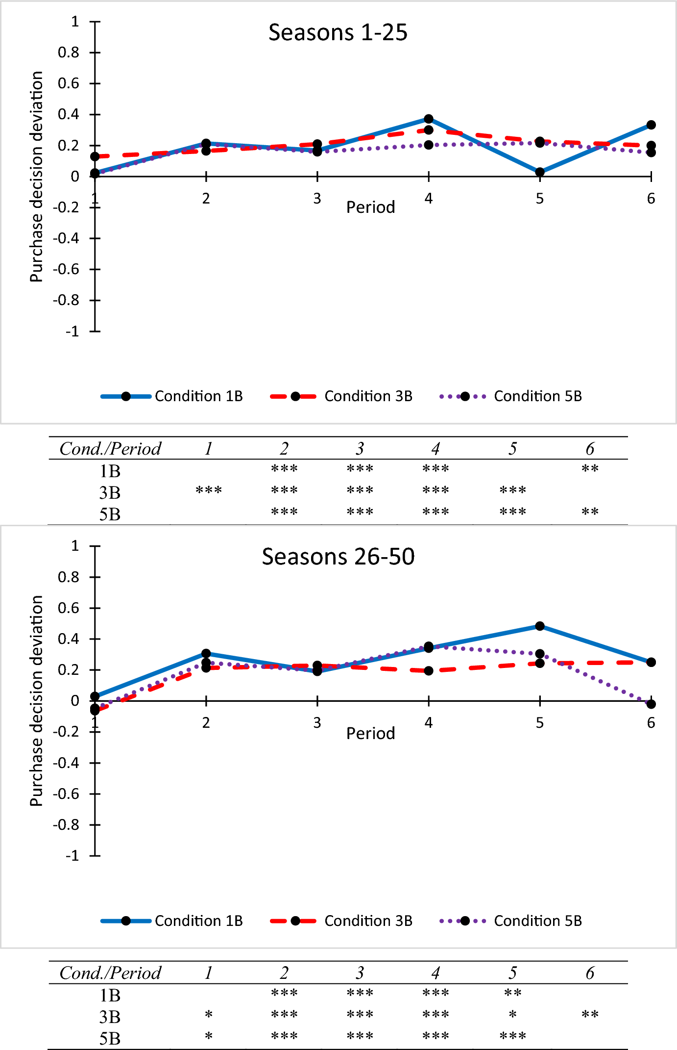
Fig. 4 Mean deviation of experimental Consumer purchase decisions from best response according to equilibrium analysis. The unit of analysis is the session. The accompanying tables serve the same function with the same notation as those for Fig. 3
4.3 Difference between conditions and within-session evolution
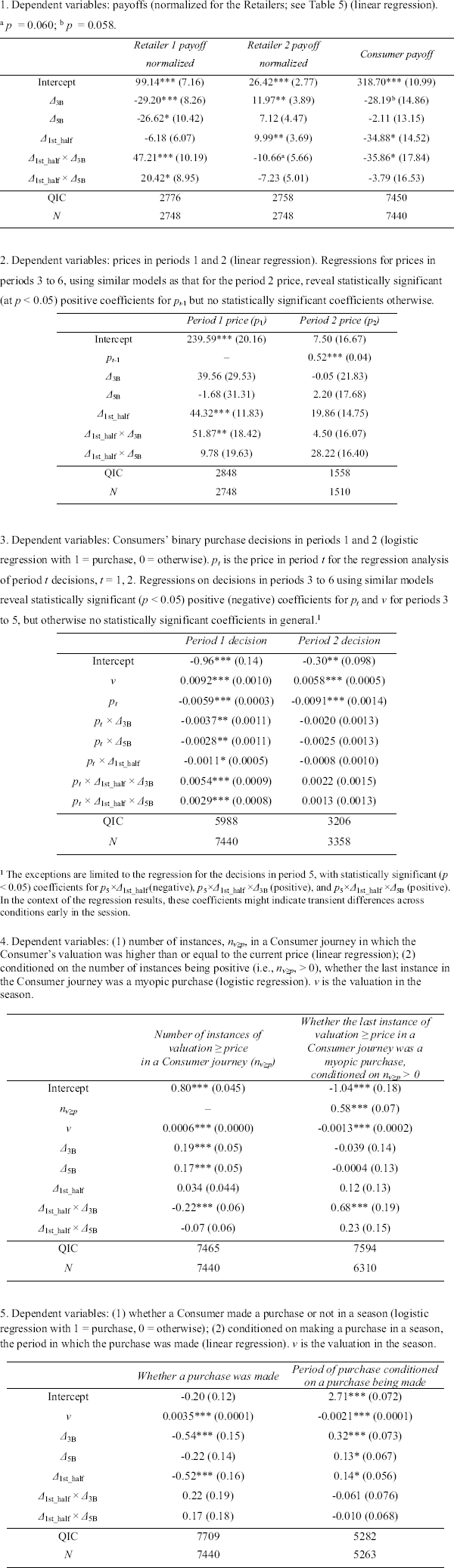
Our final set of analysis involves a direct comparison between conditions and examination of within-session evolution. The analysis involves regressions with results that are displayed in Table 6.
Table 6 Regression analysis results. Variances are clustered by subjects. Standard errors in parentheses. The QIC goodness-of-fit statistic is also listed. Where the estimated coefficient is significantly different from zero, the coefficient is indicated by one or more asterisks (*p < 0.05; **p < 0.01; ***p < 0.001). Δ 3B = 1 when the data point is from Condition 3B and Δ 3B = 0 otherwise; Δ 5B = 1 when the data point is from Condition 5B and Δ 5B = 0 otherwise. In addition, Δ 1st_half = 1 when the data point is from Seasons 1–25 and Δ 1st_half = 0 otherwise. Further specific details for each panel are provided in the respective headings
|
The exceptions are limited to the regression for the decisions in period 5, with statistically significant (p < 0.05) coefficients for p 5 × Δ 1st_half (negative), p 5 × Δ 1st_half × Δ 3B (positive), and p 5 × Δ 1st_half × Δ 5B (positive). In the context of the regression results, these coefficients might indicate transient differences across conditions early in the session
a p = 0.060; b p = 0.058
The first panel of Table 6, regarding the payoffs, indicates that the theoretical invariance with respect to the number of consumers was violated. For example, focusing on the latter half of the session (i.e., when Δ 1st_half = 0 following the terminology for Table 6), Retailer 1's payoffs in Condition 1B was less than its payoffs in the other two conditions, even after normalization by the number of Consumers. Retailer 2, on the other hand, earned a higher payoff in Condition 3B than in Condition 1B.
However, the second panel of Table 6 shows that the Retailers’ prices were not significantly different across conditions in the latter part of the session, suggesting that the violation of invariance might not be attributable to prices.
Rather, as evidenced in the third panel of Table 6, Consumers seemed to be more prone to attempt strategic waiting in period 1 in Conditions 3B and 5B than in Condition 1B, at least in the latter half of the session. This is consistent with earlier results as in Fig. 4. This could help to explain Retailer 1's lower normalized payoffs in Conditions 3B and 5B relative to Condition 1B. The panel also shows a lack of corresponding differences in strategic waiting tendency across conditions in period 2. That is, while a higher number of Consumers might prompt Consumers to attempt strategic waiting in period 1, this tendency did not persist into period 2—and beyond, as our analysis for other periods also suggests.
Another analysis approach, summarized in the fourth panel of Table 6, provides corroborating evidence. If Consumers attempted more strategic waiting in Conditions 3B and 5B than in Condition 1B, there should be correspondingly more instances per Consumer journey where the Consumer's valuation was higher than or equal to the current price. This is because the Consumer became more likely to attempt strategic waiting in such instances and continue the journey without making a purchase. The middle column results of Table 6's fourth panel indeed shows that there was a larger number of instances of such—which we denote as n v≥p —in Condition 3B (at least in the second half of the session) and Condition 5B, compared with Condition 1B. It is also interesting to see whether, conditioned on n v≥p being positive, the last instance where “valuation ≥ price” was a myopic purchase, which is defined as making a purchase when the best response should be the opposite. The logistic regression results summarized in the right column in Table 6's fourth panel essentially show that, across condition, myopic purchase became more likely the larger number of times the Consumer had attempted strategic waiting in the same Consumer journey. This seeming inconsistency could be due to a simple heuristic that the Consumer only allowed themselves to “miss making a profit” (i.e., waiting despite valuation ≥ price) a limited number of times within a Consumer journey; more research might be warranted to find out the in-depth behavioral reasons behind.
Finally, Table 6's fifth panel provides further evidence on Consumer purchase that is consistent with the above findings. The analysis shows that, in the latter half of the session, the higher a Consumers’ valuation, the more likely they were to make a purchase in a season, and conditioned on a purchase being made, the lower the number of periods at which the purchase occurred. Moreover, the likelihood to purchase was lower in Condition 3B than in Condition 1B controlling for the valuation, and the purchase period in Conditions 3B and 5B relative to 1B was higher controlling for the valuation, suggesting a higher tendency to attempt strategic waiting in those conditions.
Table 6's panels also illustrate clearly that there was within-session evolution. For example, consistent with Fig. 3, Table 6's panel 2 shows that period 1 prices were overall driven down in the latter half of the session. In parallel, Table 6's panels 3 and 5 (and panel 4 also with partial evidence for Condition 3B), show that there was an increased tendency for strategic waiting among Consumers as the session progressed.Footnote 5
Table 7 helps to drive home the insights from the Table 6 regression results on Consumer decisions. Table 7 shows the frequency distributions of Consumer journeys distinguished by whether the Consumer made one of four types of ex post suboptimal decisions in the season (i.e., decisions that were suboptimal vis a vis the ex post observations of the full set of posted prices by Retailers in a season after the season was over):
(1) Purchase with negative payoff;
(2) Purchase with non-negative payoff but ex post “too early,” which denotes purchasing in a period after which there is at least one period in the same season when the price is lower;
(3) Purchase with non-negative payoff but ex post “too late,” which denotes purchasing at a price that is higher than previous prices in the same seasonFootnote 6;
(4) No-purchase (that is ex post suboptimal), which denotes not purchasing before the season terminates although at least one price during the season is below the Consumer's valuation.
Table 7 Percentages of Consumer journeys distinguished by the ex post (sub)optimality of the purchase timing (absolute frequencies in parentheses) (see Sect. 4.3)

|
Ex post suboptimal |
Ex post optimal |
|||||
|---|---|---|---|---|---|---|
|
Purchase |
No-purchase |
Purchase |
No-purchase |
|||
|
Payoff < 0 |
Payoff ≥ 0, “too early” |
Payoff ≥ 0, “too late” |
“too late” |
|||
|
Condition 1B |
0.08 (1) |
NA |
0 (0) |
12.42 (149) |
74.17 (890) |
13.33 (160) |
|
Condition 3B |
0.22 (5) |
26.40 (594) |
0.18 (4) |
16.58 (373) |
39.82 (896) |
16.80 (378) |
|
Condition 5B |
0.58 (23) |
35.94 (1434) |
0.03 (1) |
14.26 (569) |
35.46 (1415) |
13.73 (548) |
The total count in each condition is: Condition 1B: 1200; Condition 3B: 2250; Condition 5b: 3990
In addition, Table 7 shows the frequency distributions of Consumer journeys in which the Consumer made one of two types of ex post optimal decision:
(1) Purchase at a price that turns out to be the lowest in the season and is not higher than the Consumer's valuation;
(1) No-purchase (that is ex post optimal), which denotes not purchasing in a season in which all the prices are higher than the Consumer's valuation.
Table 7 highlights how Conditions 3B and 5B made possible a substantial number of observations of ex post “too early” purchases that were not possible by design in Condition 1B (as there was only one Consumer in the market in Condition 1B). At the same time, there were lower proportions of ex post optimal purchases in Conditions 3B and 5B, as the season could continue often at lower prices after a Consumer had purchased. All these instances could motivate Consumers to attempt more strategic waiting. The difference in observations between ex post “too early” and ex post “too late”, in Conditions 3B and 5B, was such that there were about twice as many observations of ex post “too early” as ex post “too late”. The observations might have motivated Consumer players to behave more patiently and to attempt to strategically delay purchase compared to the Condition 1B, where only ex post “too late” observations were possible.
5 Conclusions
In this research, we introduce and test a stylized model of dynamic pricing under duopolistic competition. Our model extends previous work on zigzag competition (MGG and MRG, as discussed earlier) in which a consumer receives alternating price offers between two retailers over an indefinite horizon with random continuation probability, or equivalently, infinite horizon with identical per period time discount factor across players. Our equilibrium analysis suggests that price offers decrease exponentially across periods over the season. Moreover, the theoretical predictions are invariant with respect to the number of consumers in the game, as long as their valuations are ex ante independently and identically distributed.
Our experiment demonstrated significant deviations from equilibrium predictions that exhibited consistent and different characteristics from the related previous results from MRG's finite-horizon experimental study. In our experiment, Retailers often overpriced relative to equilibrium benchmarks, a result that is similar to MRG's results. However, overpricing in MRG persisted throughout the experimental session while it became mitigated in our indefinite-horizon case.
Moreover, the theoretical invariance with respect to the number of consumers was violated (a research objective that MRG did not study). As the number of Consumers increased, Consumers in the experiment became more prone to strategic waiting and exhibited less myopic behavior. This led to a decrease in the per-Consumer payoff of Retailer 1 in Conditions 3B and 5B compared with 1B. However, the increase in strategic waiting did not seem to extend beyond period 1, and a corresponding increase in per-consumer payoff of Retailer 2. Moreover, despite such relative increase in strategic waiting in period 1 across conditions, Consumers were generally not sufficiently strategic when compared to theoretical benchmarks. Hence, similar to the Strategic conditions in MRG, we find that the second Retailer generally earned more than predicted by equilibrium analysis, while the first Retailer and the Consumers generally did worse than predicted by equilibrium analysis.
Such findings are in line with the second possible reason discussed in the Introduction section of this paper regarding why the theoretical invariance with respect to the number of consumers could be violated behaviorally. That is, as the number of Consumers increased, players expected that the market would take longer to clear and the season would last longer, resulting in an increased tendency for strategic behavior. Our experimental findings also shed insights into the validity of the other reasons discussed. For example, the first reason discussed in the Introduction is the possibility that Consumers were heterogeneous in terms of how myopic they were. As the number of Consumer increased across conditions, the probability that at least one Consumer was myopic increased, and Retailers might adjust their pricing strategies accordingly. If this adjustment approach was indeed practiced by the Retailers, we might expect to see increases in prices as the number of Consumers increased—which, however, is not supported by our data analysis (e.g., the second panel of Table 6). Another reason suggested in the Introduction is related to the possibility that Consumers might be affected by social comparison effects when there were multiple of them, such as fairness concerns and socially induced regret (when, e.g., another Consumer purchased at a better price). Retailers anticipating these concerns might adjust their pricing strategies such that prices across periods and Retailers might be more equal as the number of Consumers increased. However, we do not find evidence in support this possibility. For example, the second panel of Table 6 suggests that the difference between prices in periods 1 and 2 did not decrease as the number of Consumers increased.
Lastly, our analysis suggests evidence of within-session evolution, in that the Retailers’ overpricing tendency decreased over the experimental session. This is consistent with competitive pressure driving down prices that got closer to equilibrium predictions. Correspondingly, there was an increased tendency for strategic waiting among Consumers as the session progressed.
Our work can be extended in a number of directions. Further experimentation could be carried out that elicits subject beliefs and/or decision rationale in order to estimate more detailed behavioral models for decisions, test further behavioral predictions, and, in general, find out more about the behavioral factors behind the deviations from theoretical predictions. Another possible direction pertains to the information structure, a direction that MRG also explored. In particular, MRG replaced their main modelling assumption that once a price is posted it is observed by the consumer and the two retailers, by the assumption that Retailer 1 never observes the price offers made by Retailer 2 and vice versa. The effect of this change from complete to incomplete information is quite dramatic, as MRG have proved that if information about prices is restricted in this sense, trade occurs at only zero price in equilibrium. In effect, competition between the two retailers is highly intensified when they cannot monitor each other's prices, and the result becomes the classical Bertrand outcome. An implication of this result is that both retailers would be willing to pay cash in order to gain full transparency of the market. In the present model, because the horizon does not have a fixed finite number of periods as in MRG, it can be expected that the equilibrium analysis will not result in a state of Bertrand outcome with all profits competed away. In yet another direction, the zigzag competition assumption can be relaxed so that the consumer(s) could switch between retailers with a probability that is between 0 and 1; a first step could be to model this probability as exogenous and constant as in a simple first order Markov process (see MGG). Lastly, to study and isolate specific responses, Retailer or Consumer subjects may be replaced with computerized robots playing different strategies (equilibrium or other). Further theoretical and experimental explorations might reveal more insights into competitive dynamic pricing behavior.
Supplementary Information
The online version contains supplementary material available at https://doi.org/10.1007/s10683-024-09848-8.
Acknowledgements
Eyran J. Gisches, Vincent Mak, and Rami Zwick would like to honor Amnon Rapoport with this paper and express their gratitude to Amnon's advice, collaboration, and friendship over the years. Gisches, Mak, and Zwick are responsible for any errors in the paper.
Funding
This study was supported by University of California, Riverside.
Declarations
Competing interests
The authors declare that they have no conflicts of interest with respect to their authorship or the publication of this article.


 Open access