


1 Introduction
Machine learning and artificial intelligence play a major role in today’s society: self-driving cars (e.g. [Reference Bachute and Subhedar3]), automated medical diagnoses (e.g. [Reference Rajkomar, Dean and Kohane41]) and security systems based on face recognition (e.g. [Reference Sharma, Bhatt and Sharma45]), for instance, are often based on certain machine learning models, such as deep neural networks (DNNs). DNNs often approximate functions that are discontinuous with respect to their input [Reference Szegedy, Zaremba, Sutskever, Bruna, Erhan, Goodfellow and Fergus48] making them susceptible to so-called adversarial attacks. In an adversarial attack, an adversary aims to change the prediction of a DNN through a directed, but small perturbation to the input. We refer to [Reference Goodfellow, Shlens and Szegedy14] for an example showing the weakness of DNNs towards adversarial attacks. Especially when employing DNNs in safety-critical applications, the training of machine learning models in a way that is robust to adversarial attacks has become a vital task.
Machine learning models are usually trained by minimising an associated loss function. In adversarially robust learning, this loss function is considered to be subject to adversarial attacks. The adversarial attack is usually given by a perturbation of the input data that is chosen to maximise the loss function. Thus, adversarial robust learning is formulated as a minmax optimisation problem. In practice, the inner maximisation problem needs to be approximated: [Reference Goodfellow, Shlens and Szegedy14] proposed the fast gradient sign method (FGSM), which perturbs the input data to maximise the loss function with a single step. Improvements of FGSM were proposed by, e.g. [Reference Kurakin, Goodfellow and Bengio25, Reference Tramèr, Kurakin, Papernot, Goodfellow, Boneh and McDaniel51, Reference Wong, Rice and Kolter57]. Another popular methodology is projected gradient descent (PGD) [Reference Madry, Makelov, Schmidt, Tsipras and Vladu32] and its variants, see, for example, [Reference Croce and Hein9, Reference Dong, Liao, Pang, Su, Zhu, Hu and Li10, Reference Maini, Wong, Kolter, H. and Singh33, Reference Mosbach, Andriushchenko, Trost, Hein and Klakow36, Reference Tramer and Boneh50, Reference Yang, Zhang, Katabi and Xu61]. Similar to FGSM, PGD considers the minmax optimisation problem but uses multi-step gradient ascent to approximate the inner maximisation problem. Notably, [Reference Wong, Rice and Kolter57] showed that FGSM with random initialisation is as effective as PGD.
Other defense methods include preprocessing (e.g. [Reference Guo, Rana, Cisse and van der Maaten16, Reference Song, Kim, Nowozin, Ermon and Kushman47, Reference Xu, Evans and Qi59, Reference Yun, Han, Chun, Oh, Yoo and Choe63]) and detection (e.g. [Reference Carlini and Wagner5, Reference Liu, Levine, Lau, Chellappa and Feizi31, Reference Metzen, Genewein, Fischer and Bischoff35, Reference Xu, Xiao, Zheng, Cai and Nevatia58]), as well as provable defenses (e.g. [Reference Gowal, Dvijotham, Stanforth, Bunel, Qin, Uesato, Arandjelovic, Mann and Kohli15, Reference Jia, Qu and Gong21, Reference Sheikholeslami, Lotfi and Kolter46, Reference Wong and Kolter55]). Various attack methods have also been proposed, see, for instance, [Reference Carlini and Wagner6, Reference Croce and Hein9, Reference Ghiasi, Shafahi and Goldstein13, Reference Wong, Schmidt and Kolter56]. More recently, there is an increased focus on using generative models to improve adversarial accuracy, see for example [Reference Nie, Guo, Huang, Xiao, Vahdat and Anandkumar38, Reference Wang, Pang, Du, Lin, Liu and Yan54, Reference Xue, Araujo, Hu and Chen60].
In the present work, we study the case of an adversary that finds their attack following a Bayesian statistical methodology. The Bayesian adversary does not find the attack through optimisation, but by sampling a probability distribution that can be derived using Bayes’ Theorem. Importantly, we study the setting in which the adversary uses a Bayesian strategy, but the machine learner/defender trains the model using optimisation, which is in contrast to [Reference Ye, Zhu, Bengio, Wallach, Larochelle, Grauman, Cesa-Bianchi and Garnett62]. Thus, our ansatz is orthogonal to previous studies of adversarial robustness by assuming that the attacker uses a significantly different technique. On the other hand, the associated Bayesian adversarial robustness problem can be interpreted as a stochastic relaxation of the classical minmax problem that replaces the inner maximisation problem with an integral. Thus, our ansatz should also serve as an alternative way to approach the computationally challenging minmax problem with a sampling based strategy. After establishing these connections, we
-
• propose Abram (short for Adversarial Bayesian Particle Sampler), a particle-based continuous-time dynamical system that simultaneously approximates the behaviour of the Bayesian adversary and trains the model via gradient descent.
Particle systems of this form have been used previously to solve such optimisation problems in the context of maximum marginal likelihood estimation, see, e.g. [Reference Johnston, Crucinio, Akyildiz, Sabanis and Girolami2] and [Reference Kuntz, Lim and Johansen24]. In order to justify the use Abram in this situation, we
-
• show that Abram converges to a McKean–Vlasov stochastic differential equation (SDE) as the number of particles goes to infinity, and
-
• give assumptions under which the McKean–Vlasov SDE converges to the minimiser of the Bayesian adversarial robustness problem with an exponential rate.
Additional complexity arises here compared to earlier work as the dynamical system and its limiting McKean–Vlasov SDE have to be considered under reflecting boundary conditions. After the analysis of the continuous-time system, we briefly explain its discretisation. Then, we
-
• compare Abram to the state of the art in adversarially robust classification of the MNIST and the CIFAR-10 datasets under various kinds of attacks.
This work is organised as follows. We introduce the (Bayesian) adversarial robustness problem in Section 2 and the Abram method in Section 3. We analyse Abram in Sections 4 (large particle limit) and 5 (longtime behaviour). We discuss different ways of employing Abram in practice in Section 6 and compare it to the state of the art in adversarially robust learning in Section 7. We conclude in Section 8.
2 Adversarial robustness and its Bayesian relaxation
In the following, we consider a supervised machine learning problem of the following form. We are given a training dataset
 $\{(y_1, z_1),\ldots, (y_K, z_K)\}$
of pairs of features
$\{(y_1, z_1),\ldots, (y_K, z_K)\}$
of pairs of features
 $y_1,\ldots, y_K \in Y \,:\!=\,\mathbb {R}^{d_Y}$
and labels
$y_1,\ldots, y_K \in Y \,:\!=\,\mathbb {R}^{d_Y}$
and labels
 $z_1,\ldots, z_K \in Z$
. Moreover, we are given a parametric model of the form
$z_1,\ldots, z_K \in Z$
. Moreover, we are given a parametric model of the form
 $g: X \times Y \rightarrow Z$
, with
$g: X \times Y \rightarrow Z$
, with
 $X \,:\!=\, \mathbb {R}^d$
denoting the parameter space. The goal is now to find a parameter
$X \,:\!=\, \mathbb {R}^d$
denoting the parameter space. The goal is now to find a parameter
 $\theta ^*$
, for which
$\theta ^*$
, for which
 \begin{equation*} g(y_k|\theta ^*) \approx z_k \qquad (k=1,\ldots, K). \end{equation*}
In practice the function
 $g(\!\cdot |\theta ^*)$
shall then be used to predict labels of features (especially such outside of training dataset).
$g(\!\cdot |\theta ^*)$
shall then be used to predict labels of features (especially such outside of training dataset).
The parameter
 $\theta ^*$
is usually found through optimisation. Let
$\theta ^*$
is usually found through optimisation. Let
 $\mathcal {L}:Z \times Z \rightarrow \mathbb {R}$
denote a loss function – a function that gives a reasonable way of comparing the output of
$\mathcal {L}:Z \times Z \rightarrow \mathbb {R}$
denote a loss function – a function that gives a reasonable way of comparing the output of
 $g$
with observed labels. Usual examples are the square loss for continuous labels and cross entropy loss for discrete labels. Then, we need to solve the following optimisation problem:
$g$
with observed labels. Usual examples are the square loss for continuous labels and cross entropy loss for discrete labels. Then, we need to solve the following optimisation problem:
 \begin{align} \min _{\theta \in X} & \frac {1}{K}\sum _{k=1}^K \Phi (y_k,z_k|\theta ), \end{align}
where
 $\Phi (y,z|\theta ) \,:\!=\, \mathcal {L}(g(y|\theta ),z)$
.
$\Phi (y,z|\theta ) \,:\!=\, \mathcal {L}(g(y|\theta ),z)$
.
Machine learning models
 $g$
that are trained in this form are often susceptible to adversarial attacks. That means, for a given feature vector
$g$
that are trained in this form are often susceptible to adversarial attacks. That means, for a given feature vector
 $y$
, we can find a ‘small’
$y$
, we can find a ‘small’
 $\xi \in Y$
for which
$\xi \in Y$
for which
 $g(y+\xi |\theta ^*) \neq g(y|\theta ^*)$
. In this case, an adversary can change the model’s predicted label by a very slight alteration of the input feature. Such a
$g(y+\xi |\theta ^*) \neq g(y|\theta ^*)$
. In this case, an adversary can change the model’s predicted label by a very slight alteration of the input feature. Such a
 $\xi$
can usually be found through optimisation on the input domain:
$\xi$
can usually be found through optimisation on the input domain:
 \begin{equation*}\max _{\xi \in B(\varepsilon )}\Phi (y+\xi, z|\theta ),\end{equation*}
where
 $B(\varepsilon ) = \{\xi : \|\xi \|\leq \varepsilon \}$
denotes the
$B(\varepsilon ) = \{\xi : \|\xi \|\leq \varepsilon \}$
denotes the
 $\varepsilon$
-ball centred at
$\varepsilon$
-ball centred at
 $0$
and
$0$
and
 $\varepsilon \gt 0$
denotes the size of the adversarial attack. Hence, the attacker tries to change the prediction of the model whilst altering the model input only by a small value
$\varepsilon \gt 0$
denotes the size of the adversarial attack. Hence, the attacker tries to change the prediction of the model whilst altering the model input only by a small value
 $\leq \varepsilon$
. Other kinds of attacks are possible, the attacker may, e.g. try to not only change the predicted label to any other label, but rather to a particular target label, see, e.g. [Reference Kurakin, Goodfellow and Bengio26].
$\leq \varepsilon$
. Other kinds of attacks are possible, the attacker may, e.g. try to not only change the predicted label to any other label, but rather to a particular target label, see, e.g. [Reference Kurakin, Goodfellow and Bengio26].
In adversarially robust training, we replace the optimisation problem (2.1) by the minmax optimisation problem below:
 \begin{equation} \min _{\theta \in X} \frac {1}{K}\sum _{k=1}^K \max _{\xi _k \in B(\varepsilon )}\Phi (y_k+\xi _k,z_k|\theta ). \end{equation}
Thus, we now train the network by minimising the loss also with respect to potential adversarial attacks. Finding the accurate solutions to such minmax optimisation problems is difficult: usually there is no underlying saddlepoint structure, e.g.
 $\Phi (y,z|\theta )$
is neither convex in
$\Phi (y,z|\theta )$
is neither convex in
 $\theta$
nor concave in
$\theta$
nor concave in
 $y$
,
$y$
,
 $X$
and
$X$
and
 $Y$
tend to be very high-dimensional spaces, and the number of data points
$Y$
tend to be very high-dimensional spaces, and the number of data points
 $K$
may prevent the accurate computation of gradients. However, good heuristics have been established throughout the last decade – we have mentioned some of them in Section 1.
$K$
may prevent the accurate computation of gradients. However, good heuristics have been established throughout the last decade – we have mentioned some of them in Section 1.
In this work, we aim to study a relaxed version of the minmax problem, which we refer to as the Bayesian adversarial robustness problem. This problem is given by
 \begin{equation} \min _{\theta \in X} \frac {1}{K}\sum _{k =1}^K \int _{B({\varepsilon })} \Phi (y_k+\xi _k,z_k|\theta ) \pi ^{\gamma, \varepsilon }_k(\mathrm {d}\xi _k|\theta ), \end{equation}
where the Bayesian adversarial distribution
 $\pi ^{\gamma, \varepsilon }_k(\cdot |\theta )$
has (Lebesgue) density
$\pi ^{\gamma, \varepsilon }_k(\cdot |\theta )$
has (Lebesgue) density
 \begin{equation*} \xi \mapsto \frac {\exp (\gamma \Phi (y_k+\xi, z_k|\theta )) \mathbf {1}[\xi \in B(\varepsilon )]}{\int _{B(\varepsilon )} \exp (\gamma \Phi (y_k+\xi ',z_k|\theta )) \mathrm {d}\xi '}, \end{equation*}
where
 $\gamma \gt 0$
is an inverse temperature,
$\gamma \gt 0$
is an inverse temperature,
 $\varepsilon \gt 0$
still denotes the size of the adversarial attack, and
$\varepsilon \gt 0$
still denotes the size of the adversarial attack, and
 $\mathbf {1}[\cdot ]$
denotes the indicator:
$\mathbf {1}[\cdot ]$
denotes the indicator:
 $\mathbf {1}[\mathrm {true}] \,:\!=\, 1$
and
$\mathbf {1}[\mathrm {true}] \,:\!=\, 1$
and
 $\mathbf {1}[\mathrm {false}] \,:\!=\, 0$
. The distribution
$\mathbf {1}[\mathrm {false}] \,:\!=\, 0$
. The distribution
 $\pi ^{\gamma, \varepsilon }_k(\cdot |\theta )$
is concentrated on the
$\pi ^{\gamma, \varepsilon }_k(\cdot |\theta )$
is concentrated on the
 $\varepsilon$
-ball,
$\varepsilon$
-ball,
 $\varepsilon \gt 0$
controls the range of the attack,
$\varepsilon \gt 0$
controls the range of the attack,
 $\gamma \gt 0$
controls its focus. We illustrate this behaviour in Figure 1. Next, we comment on the mentioned relaxation and the Bayesian derivation of this optimisation problem.
$\gamma \gt 0$
controls its focus. We illustrate this behaviour in Figure 1. Next, we comment on the mentioned relaxation and the Bayesian derivation of this optimisation problem.

Figure 1.
Plots of the Lebesgue density of
 $\pi _1^{\gamma, \varepsilon }(\cdot |\theta _0)$
for energy
$\pi _1^{\gamma, \varepsilon }(\cdot |\theta _0)$
for energy
 $\Phi (y_1 + \xi, z_1|\theta _0) = (\xi -0.1)^2/2$
, choosing parameters
$\Phi (y_1 + \xi, z_1|\theta _0) = (\xi -0.1)^2/2$
, choosing parameters
 $\varepsilon \in \{0.025, 0.1, 0.4\}$
and
$\varepsilon \in \{0.025, 0.1, 0.4\}$
and
 $\gamma \in \{0.1, 10, 1000\}$
.
$\gamma \in \{0.1, 10, 1000\}$
.
2.1 Relaxation
Under certain assumptions,Footnote 1 one can show that
 \begin{equation*}\pi ^{\gamma, \varepsilon }_k(\cdot |\theta ) \rightarrow \mathrm {Unif}(\mathrm {argmax}_{\xi \in Y} \Phi (y_k + \xi, z_k|\theta ))\end{equation*}
weakly as
 $\gamma \rightarrow \infty$
, see [Reference Hwang20]. Indeed, the Bayesian adversarial distribution converges to the uniform distribution over the global maximisers computed with respect to the adversarial attack. This limiting behaviour, that we can also see in Figure 1, forms the basis of simulated annealing methods for global optimisation. Moreover, it implies that the optimisation problems (2.2) and (2.3) are identical in the limit
$\gamma \rightarrow \infty$
, see [Reference Hwang20]. Indeed, the Bayesian adversarial distribution converges to the uniform distribution over the global maximisers computed with respect to the adversarial attack. This limiting behaviour, that we can also see in Figure 1, forms the basis of simulated annealing methods for global optimisation. Moreover, it implies that the optimisation problems (2.2) and (2.3) are identical in the limit
 $\gamma \to \infty$
, since
$\gamma \to \infty$
, since
 \begin{align*} \lim _{\gamma \rightarrow \infty } \frac {1}{K}\sum _{k =1}^K &\int _{B({\varepsilon })} \Phi (y_k+\xi _k,z_k|\theta ) \pi ^{\gamma, \varepsilon }_k(\mathrm {d}\xi _i|\theta ) \\ &= \frac {1}{K}\sum _{k =1}^K \int _{B({\varepsilon })} \Phi (y_k+\xi _k,z_k|\theta ) \mathrm {Unif}(\mathrm {argmax}_{\xi \in Y} \Phi (y_k + \xi, z_k|\theta ))(\mathrm {d}\xi _i), \end{align*}
and since
 $\xi _k \sim \mathrm {Unif}(\mathrm {argmax}_{\xi \in Y} \Phi (y_k + \xi, z_k|\theta ))$
implies
$\xi _k \sim \mathrm {Unif}(\mathrm {argmax}_{\xi \in Y} \Phi (y_k + \xi, z_k|\theta ))$
implies
 $\Phi (y_k+\xi _k,z_k|\theta ) = \max _{\xi \in B(\varepsilon )}\Phi (y_k+\xi, z_k|\theta )$
almost surely for
$\Phi (y_k+\xi _k,z_k|\theta ) = \max _{\xi \in B(\varepsilon )}\Phi (y_k+\xi, z_k|\theta )$
almost surely for
 $k =1,\ldots, K$
. A strictly positive
$k =1,\ldots, K$
. A strictly positive
 $\gamma$
on the other hand leads to a relaxed problem circumventing the minmax optimisation. [Reference Cipriani, Scagliotti and Wöhrer8] have also discussed this relaxation of an adversarial robustness problem in the context of a finite set of attacks, i.e. the
$\gamma$
on the other hand leads to a relaxed problem circumventing the minmax optimisation. [Reference Cipriani, Scagliotti and Wöhrer8] have also discussed this relaxation of an adversarial robustness problem in the context of a finite set of attacks, i.e. the
 $\varepsilon$
-ball
$\varepsilon$
-ball
 $B(\varepsilon )$
is replaced by a finite set. Probabilistically robust learning is another type of relaxation, see for example [Reference Bungert, Trillos, Jacobs, McKenzie, Nikolić and Wang4, Reference Robey, Chamon, Pappas and Hassani43]. Similar to our work, instead of doing the worst-case optimisation, i.e. finding the perturbation
$B(\varepsilon )$
is replaced by a finite set. Probabilistically robust learning is another type of relaxation, see for example [Reference Bungert, Trillos, Jacobs, McKenzie, Nikolić and Wang4, Reference Robey, Chamon, Pappas and Hassani43]. Similar to our work, instead of doing the worst-case optimisation, i.e. finding the perturbation
 $\xi$
that maximises the loss, they replace it with a probability measure on
$\xi$
that maximises the loss, they replace it with a probability measure on
 $\xi$
. This probability measure, however, follows a different paradigm.
$\xi$
. This probability measure, however, follows a different paradigm.
2.2 Bayesian attackers
We can understand the kind of attack that is implicitly employed in (2.3) as a Bayesian attack. We now briefly introduce the Bayesian learning problem to then explain its relation to this adversarial attack. In Bayesian learning, we model
 $\theta$
as a random variable with a so-called prior (distribution)
$\theta$
as a random variable with a so-called prior (distribution)
 $\pi _{\textrm { prior}}$
. The prior incorporates information about
$\pi _{\textrm { prior}}$
. The prior incorporates information about
 $\theta$
. In Bayesian learning, we now inform the prior about data
$\theta$
. In Bayesian learning, we now inform the prior about data
 $\{(y_1, z_1),\ldots, (y_K, z_K)\}$
by conditioning
$\{(y_1, z_1),\ldots, (y_K, z_K)\}$
by conditioning
 $\theta$
on that data. Indeed, we train the model by finding the conditional distribution of
$\theta$
on that data. Indeed, we train the model by finding the conditional distribution of
 $\theta$
given that
$\theta$
given that
 $g(y_k|\theta ) \approx z_k$
(
$g(y_k|\theta ) \approx z_k$
(
 $k =1,\ldots, K)$
. In the Bayesian setting, we represent ‘
$k =1,\ldots, K)$
. In the Bayesian setting, we represent ‘
 $\approx$
’ by a noise assumption consistent with the loss function
$\approx$
’ by a noise assumption consistent with the loss function
 $\mathcal {L}$
. This is achieved by defining the so-called likelihood as
$\mathcal {L}$
. This is achieved by defining the so-called likelihood as
 $\exp (\!-\Phi )$
. The conditional distribution describing
$\exp (\!-\Phi )$
. The conditional distribution describing
 $\theta$
is called the posterior (distribution)
$\theta$
is called the posterior (distribution)
 $\pi _{\textrm { post}}$
and can be obtained through Bayes’ theorem, which states that
$\pi _{\textrm { post}}$
and can be obtained through Bayes’ theorem, which states that
 \begin{equation*} \pi _{\textrm { post}}(A) = \frac {\int _A \exp \left (-\frac {1}{K}\sum _{k=1}^K\Phi (y_k, z_k|\theta )\right ) \pi _{\textrm { prior}}(\mathrm {d}\theta )}{\int _X \exp \left (-\frac {1}{K}\sum _{i=k}^K\Phi (y_k, z_k|\theta )\right ) \pi _{\textrm { prior}}(\mathrm {d}\theta )}, \end{equation*}
for measurable
 $A \subseteq X$
. A model prediction with respect to feature
$A \subseteq X$
. A model prediction with respect to feature
 $y$
can then be given by the posterior mean of the output
$y$
can then be given by the posterior mean of the output
 $g$
, which is
$g$
, which is
 \begin{equation*} \int _{{\mathbb {R}}^n} g(y|\theta ) \pi _{\textrm { post}}(\mathrm {d}\theta ). \end{equation*}
The Bayesian attacker treats the attack
 $\xi _k$
in exactly such a Bayesian way. They define a prior distribution for the attack, which is the uniform distribution over the
$\xi _k$
in exactly such a Bayesian way. They define a prior distribution for the attack, which is the uniform distribution over the
 $\varepsilon$
-ball:
$\varepsilon$
-ball:
 \begin{equation*}\mathrm {Unif}(B(\varepsilon )) = \int _{B(\varepsilon )}\mathbf {1}[\xi _k \in \cdot ]\mathrm {d}\xi _k.\end{equation*}
The adversarial likelihood is designed to essentially cancel out the likelihood in the Bayesian learning problem, by defining a function that gives small mass to the learnt prediction and large mass to anything that does not agree with the learnt prediction:
 \begin{equation*} \exp (\gamma \Phi (y_k+\xi _k,z_k|\theta )). \end{equation*}
Whilst this is not a usual likelihood corresponding to a particular noise model, we could see this as a special case of Bayesian forgetting [Reference Fu, He, Xu and Tao12]. In Bayesian forgetting, we would try to remove a single dataset from a posterior distribution by altering the distribution of the parameter
 $\theta$
. In this case, we try to alter the knowledge we could have gained about the feature vector by altering that feature vector to produce a different prediction.
$\theta$
. In this case, we try to alter the knowledge we could have gained about the feature vector by altering that feature vector to produce a different prediction.
3 Adversarial Bayesian particle sampler
We now derive a particle-based method that shall solve (2.3). To simplify the presentation in the following, we assume that
 $K=1$
, i.e. there is only a single data point. The derivation for multiple data points is equivalent – computational implications given by multiple data points will be discussed in Section 6. We also ignore the dependence of
$K=1$
, i.e. there is only a single data point. The derivation for multiple data points is equivalent – computational implications given by multiple data points will be discussed in Section 6. We also ignore the dependence of
 $\Phi$
on particular data points and note only the dependence on parameter and attack. Indeed, we write (2.3) now as
$\Phi$
on particular data points and note only the dependence on parameter and attack. Indeed, we write (2.3) now as
 \begin{equation*} \min _{\theta \in X} F(\theta ) \,:\!=\, \int _{B({\varepsilon })} \Phi (\xi, \theta ) \pi ^{\gamma, \varepsilon }(\mathrm {d}\xi |\theta ). \end{equation*}
To solve this minimisation problem, we study the gradient flow corresponding to the energy
 $F$
, that is:
$F$
, that is:
 ${\mathrm {d}\zeta _t} = -\nabla _\zeta F(\zeta _t){\mathrm {d}t}$
. The gradient flow is a continuous-time variant of the gradient descent algorithm. The gradient flow can be shown to converge to a minimiser of
${\mathrm {d}\zeta _t} = -\nabla _\zeta F(\zeta _t){\mathrm {d}t}$
. The gradient flow is a continuous-time variant of the gradient descent algorithm. The gradient flow can be shown to converge to a minimiser of
 $F$
in the longterm limit if
$F$
in the longterm limit if
 $F$
satisfies certain regularity assumptions. The gradient of
$F$
satisfies certain regularity assumptions. The gradient of
 $F$
has a rather simple expression:
$F$
has a rather simple expression:
 \begin{align*} \nabla _\theta F(\theta ) &= \nabla _\theta \frac { \int _{B(\varepsilon )}\Phi (\xi, \theta )\exp (\gamma \Phi (\xi, \theta )) \mathrm {d}\xi }{\int _{B(\varepsilon )} \exp (\gamma \Phi (\xi, \theta )) \mathrm {d}\xi } \\ &= \frac { \int _{B(\varepsilon )} \nabla _\theta \Phi (\xi, \theta ) \cdot \exp (\gamma \Phi (\xi, \theta )) + \gamma \nabla _\theta \Phi (\xi, \theta ) \cdot \Phi (\xi, \theta )\exp (\gamma \Phi (\xi, \theta )) \mathrm {d}\xi }{\int _{B(\varepsilon )} \exp (\gamma \Phi (\xi, \theta )) \mathrm {d}\xi } \\ &\qquad - \frac {\left ( \int _{B(\varepsilon )}\Phi (\xi, \theta )\exp (\gamma \Phi (\xi, \theta )) \mathrm {d}\xi \right )\left (\int _{B(\varepsilon )} \gamma \nabla _\theta \Phi (\xi, \theta ) \cdot \exp (\gamma \Phi (\xi, \theta )) \mathrm {d}\xi \right )}{\left (\int _{B(\varepsilon )}\exp (\gamma \Phi (\xi, \theta )) \mathrm {d}\xi \right )^2} \\ &= \int _{B({\varepsilon })} \nabla _\theta \Phi (\xi, \theta ) \pi ^{\gamma, \varepsilon }(\mathrm {d}\xi |\theta ) + \gamma \mathrm {Cov}_{\pi ^{\gamma, \varepsilon }(\cdot |\theta )}(\Phi (\cdot, \theta ), \nabla _\theta \Phi (\cdot, \theta )), \end{align*}
where we assume that
 $\Phi$
is continuously differentiable, bounded below and sufficiently regular to be allowed here to switch gradients and integrals. As usual, we define the covariance of appropriate functions
$\Phi$
is continuously differentiable, bounded below and sufficiently regular to be allowed here to switch gradients and integrals. As usual, we define the covariance of appropriate functions
 $f,g$
with respect to a probability distribution
$f,g$
with respect to a probability distribution
 $\pi$
, by
$\pi$
, by
 \begin{equation*} \mathrm {Cov}_{\pi }(f,g) \,:\!=\, \int _X f(\theta )g(\theta ) \pi (\mathrm {d}\theta ) - \int _X f(\theta ) \pi (\mathrm {d}\theta )\int _X g(\theta ) \pi (\mathrm {d}\theta ). \end{equation*}
The structure of
 $\nabla _\theta F$
is surprisingly simple, requiring only integrals of the target function and its gradient with respect to
$\nabla _\theta F$
is surprisingly simple, requiring only integrals of the target function and its gradient with respect to
 $\pi ^{\gamma, \varepsilon }$
, but, e.g. not its normalising constant. In practice, it is usually not possible to compute these integrals analytically or to even sample independently from
$\pi ^{\gamma, \varepsilon }$
, but, e.g. not its normalising constant. In practice, it is usually not possible to compute these integrals analytically or to even sample independently from
 $\pi ^{\gamma, \varepsilon }(\cdot |\theta )$
, which would be necessary for a stochastic gradient descent approach. The latter approach first introduced by [Reference Robbins and Monro42] allows the minimisation of expected values by replacing these expected values by sample means; see also [Reference Jin, Latz, Liu and Schönlieb22] and [Reference Latz28] for continuous-time variants. Instead, we use a particle system approach that has been studied for a different problem by [Reference Johnston, Crucinio, Akyildiz, Sabanis and Girolami2] and [Reference Kuntz, Lim and Johansen24]. The underlying idea is to approximate
$\pi ^{\gamma, \varepsilon }(\cdot |\theta )$
, which would be necessary for a stochastic gradient descent approach. The latter approach first introduced by [Reference Robbins and Monro42] allows the minimisation of expected values by replacing these expected values by sample means; see also [Reference Jin, Latz, Liu and Schönlieb22] and [Reference Latz28] for continuous-time variants. Instead, we use a particle system approach that has been studied for a different problem by [Reference Johnston, Crucinio, Akyildiz, Sabanis and Girolami2] and [Reference Kuntz, Lim and Johansen24]. The underlying idea is to approximate
 $\pi ^{\gamma, \varepsilon }(\cdot |\theta )$
by an overdamped Langevin dynamics, which is restricted to the
$\pi ^{\gamma, \varepsilon }(\cdot |\theta )$
by an overdamped Langevin dynamics, which is restricted to the
 $\varepsilon$
-Ball
$\varepsilon$
-Ball
 $B(\varepsilon )$
with reflecting boundary conditions:
$B(\varepsilon )$
with reflecting boundary conditions:
 \begin{equation*}\mathrm {d}\xi _t = \gamma \nabla _\xi \Phi (\xi _t,\theta )\mathrm {d}t + \sqrt {2}\mathrm {d}W_t,\end{equation*}
where
 $(W_t)_{t \geq 0}$
denotes a standard Brownian motion on
$(W_t)_{t \geq 0}$
denotes a standard Brownian motion on
 $Y$
. Alternatively, one may write the dynamics as
$Y$
. Alternatively, one may write the dynamics as
 $\mathrm {d}\xi _t = \nabla _\xi \Phi (\xi _t,\theta )\mathrm {d}t + \sqrt {2/\gamma }\mathrm {d}W_t$
, which is equivalent to the current form after a time re-scaling. Under weak assumptions on
$\mathrm {d}\xi _t = \nabla _\xi \Phi (\xi _t,\theta )\mathrm {d}t + \sqrt {2/\gamma }\mathrm {d}W_t$
, which is equivalent to the current form after a time re-scaling. Under weak assumptions on
 $\Phi$
, this Langevin dynamics converges to the distribution
$\Phi$
, this Langevin dynamics converges to the distribution
 $\pi ^{\gamma, \varepsilon }(\cdot |\theta )$
as
$\pi ^{\gamma, \varepsilon }(\cdot |\theta )$
as
 $t \rightarrow \infty$
. However, due to the heavy computational costs, in practice, we are not able to simulate the longterm behaviour of this dynamics for all fixed
$t \rightarrow \infty$
. However, due to the heavy computational costs, in practice, we are not able to simulate the longterm behaviour of this dynamics for all fixed
 $\theta$
to produce samples of
$\theta$
to produce samples of
 $\pi ^{\gamma, \varepsilon }(\cdot |\theta )$
as required for stochastic gradient descent. Instead, we run a number
$\pi ^{\gamma, \varepsilon }(\cdot |\theta )$
as required for stochastic gradient descent. Instead, we run a number
 $N$
of (seemingly independent) Langevin dynamics
$N$
of (seemingly independent) Langevin dynamics
 $(\xi _t^{1,N})_{t \geq 0}, \ldots, (\xi _t^{N,N})_{t \geq 0}$
. We then obtain an approximate gradient flow
$(\xi _t^{1,N})_{t \geq 0}, \ldots, (\xi _t^{N,N})_{t \geq 0}$
. We then obtain an approximate gradient flow
 $(\theta _t^N)_{t \geq 0}$
that uses the ensemble of particles
$(\theta _t^N)_{t \geq 0}$
that uses the ensemble of particles
 $(\xi _t^{1,N})_{t \geq 0}, \ldots, (\xi _t^{N,N})_{t \geq 0}$
to approximate the expected values in the gradient
$(\xi _t^{1,N})_{t \geq 0}, \ldots, (\xi _t^{N,N})_{t \geq 0}$
to approximate the expected values in the gradient
 $\nabla _\theta F$
and then feed
$\nabla _\theta F$
and then feed
 $(\theta _t^N)_{t \geq 0}$
back into the drift of the
$(\theta _t^N)_{t \geq 0}$
back into the drift of the
 $(\xi _t^{1,N})_{t \geq 0}, \ldots, (\xi _t^{N,N})_{t \geq 0}$
. Hence, we simultaneously approximate the gradient flow
$(\xi _t^{1,N})_{t \geq 0}, \ldots, (\xi _t^{N,N})_{t \geq 0}$
. Hence, we simultaneously approximate the gradient flow
 $(\zeta _t)_{t \geq 0}$
by
$(\zeta _t)_{t \geq 0}$
by
 $(\theta ^N_t)_{t \geq 0}$
and the Bayesian adversarial distribution
$(\theta ^N_t)_{t \geq 0}$
and the Bayesian adversarial distribution
 $(\pi ^{\gamma, \varepsilon }(\cdot |\theta ^N_t))_{t \geq 0}$
by
$(\pi ^{\gamma, \varepsilon }(\cdot |\theta ^N_t))_{t \geq 0}$
by
 $(\xi _t^{1,N})_{t \geq 0}, \ldots, (\xi _t^{N,N})_{t \geq 0}$
. Overall, we obtain the dynamical system
$(\xi _t^{1,N})_{t \geq 0}, \ldots, (\xi _t^{N,N})_{t \geq 0}$
. Overall, we obtain the dynamical system
 \begin{align*} \mathrm {d}\theta _t^N &= - \frac {1}{N}\sum _{n=1}^N\nabla _\theta \Phi (\xi _t^{n,N},\theta _t^N)\mathrm {d}t - \gamma \widehat {\mathrm {Cov}}(\xi _t^N)\mathrm {d}t, \\ \mathrm {d}\xi _t^{i,N} &= \gamma \nabla _\xi \Phi (\xi _t^{i,N},\theta ^N_t)\mathrm {d}t + \sqrt {2}\mathrm {d}W_t^{i} \qquad (i =1,\ldots, N). \end{align*}
where
 $(W_t^{i})_{t \geq 0}$
are mutually independent Brownian motions on
$(W_t^{i})_{t \geq 0}$
are mutually independent Brownian motions on
 $Y$
for
$Y$
for
 $i = 1,\ldots, N$
. Again, the Langevin dynamics
$i = 1,\ldots, N$
. Again, the Langevin dynamics
 $(\xi _t^{1,N})_{t \geq 0}, \ldots, (\xi _t^{N,N})_{t \geq 0}$
are defined on the ball
$(\xi _t^{1,N})_{t \geq 0}, \ldots, (\xi _t^{N,N})_{t \geq 0}$
are defined on the ball
 $B(\varepsilon )$
with reflecting boundary conditions – we formalise this fact below. The empirical covariance is given by
$B(\varepsilon )$
with reflecting boundary conditions – we formalise this fact below. The empirical covariance is given by
 \begin{equation*}\widehat {\mathrm {Cov}}(\xi _t^N) = \frac 1{N} \sum _{i=1}^N \Phi (\xi _t^{i,N},\theta ^N_t)\nabla _\theta \Phi (\xi _t^{i,N},\theta ^N_t) - \frac 1{N^2}\sum _{i=1}^K \Phi (\xi _t^{i,N},\theta ^N_t) \sum _{j=1}^K\nabla _\theta \Phi (\xi _t^{j,N},\theta ^N_t).\end{equation*}
We refer to the dynamical system
 $(\theta ^N_t, \xi ^{1,N}_t,\ldots, \xi ^{N,N}_t)_{t \geq 0}$
as Abram. We illustrate the dynamics of Abram in Figure 2, where we consider a simple example.
$(\theta ^N_t, \xi ^{1,N}_t,\ldots, \xi ^{N,N}_t)_{t \geq 0}$
as Abram. We illustrate the dynamics of Abram in Figure 2, where we consider a simple example.

Figure 2.
Examples of the Abram method given
 $\Phi (\xi, \theta ) = \frac {1}{2}(\xi + \theta )^2$
,
$\Phi (\xi, \theta ) = \frac {1}{2}(\xi + \theta )^2$
,
 $\varepsilon = 1$
, and different combinations of
$\varepsilon = 1$
, and different combinations of
 $(\gamma, N) = (10,3)$
(top left),
$(\gamma, N) = (10,3)$
(top left),
 $(0.1,3)$
(top right),
$(0.1,3)$
(top right),
 $(10,50)$
(bottom left),
$(10,50)$
(bottom left),
 $(0.1, 50)$
(bottom right). In each of the four quadrants, we show the simulated path
$(0.1, 50)$
(bottom right). In each of the four quadrants, we show the simulated path
 $(\theta _t^N)_{t \geq 0}$
(top), the particle paths
$(\theta _t^N)_{t \geq 0}$
(top), the particle paths
 $(\xi _t^{1,N},\ldots, \xi _t^{N,N})_{t \geq 0}$
(centre), and the path of probability distributions
$(\xi _t^{1,N},\ldots, \xi _t^{N,N})_{t \geq 0}$
(centre), and the path of probability distributions
 $(\pi ^{\gamma, \varepsilon }(\cdot |\theta _t^N))_{t \geq 0}$
(bottom) that shall be approximated by the particles. The larger
$(\pi ^{\gamma, \varepsilon }(\cdot |\theta _t^N))_{t \geq 0}$
(bottom) that shall be approximated by the particles. The larger
 $\gamma$
leads to a concentration of
$\gamma$
leads to a concentration of
 $\pi ^{\gamma, \varepsilon }$
at the boundary, whilst it is closer to uniform if
$\pi ^{\gamma, \varepsilon }$
at the boundary, whilst it is closer to uniform if
 $\gamma$
is small. More particles lead to a more stable path
$\gamma$
is small. More particles lead to a more stable path
 $(\theta ^N_t)_{t \geq 0}$
. A combination of large
$(\theta ^N_t)_{t \geq 0}$
. A combination of large
 $N$
and
$N$
and
 $\gamma$
leads to convergence to the minimiser
$\gamma$
leads to convergence to the minimiser
 $\theta _* = 0$
of
$\theta _* = 0$
of
 $F$
.
$F$
.
We have motivated this particle system as an approximation to the underlying gradient flow
 $(\zeta _t)_{t \geq 0}$
. As
$(\zeta _t)_{t \geq 0}$
. As
 $N \rightarrow \infty$
, the dynamics
$N \rightarrow \infty$
, the dynamics
 $(\theta ^N_t)_{t \geq 0}$
does not necessarily convergence to the gradient flow
$(\theta ^N_t)_{t \geq 0}$
does not necessarily convergence to the gradient flow
 $(\zeta _t)_{t \geq 0}$
, but to a certain McKean–Vlasov stochastic differential equation (SDE), see [Reference McKean34]. We study this convergence behaviour in the following, as well as the convergence of the McKean–Vlasov SDE to the minimiser of
$(\zeta _t)_{t \geq 0}$
, but to a certain McKean–Vlasov stochastic differential equation (SDE), see [Reference McKean34]. We study this convergence behaviour in the following, as well as the convergence of the McKean–Vlasov SDE to the minimiser of
 $F$
and, thus, justify Abram as a method for Bayesian adversarial learning. First, we introduce the complete mathematical set-up and give required assumptions. To make it easier for the reader to keep track of the different stochastic processes that appear throughout this work, we summarise them in Table 1.
$F$
and, thus, justify Abram as a method for Bayesian adversarial learning. First, we introduce the complete mathematical set-up and give required assumptions. To make it easier for the reader to keep track of the different stochastic processes that appear throughout this work, we summarise them in Table 1.
Table 1. Definitions of stochastic processes throughout this work

3.1 Mean-field limit
In the following, we are interested in the mean field limit of Abram, i.e. we analyse the limit of
 $(\theta ^N_t)_{t \geq 0}$
as
$(\theta ^N_t)_{t \geq 0}$
as
 $N \rightarrow \infty$
. Thus, we can certainly assume for now that
$N \rightarrow \infty$
. Thus, we can certainly assume for now that
 $\gamma \,:\!=\, 1$
and
$\gamma \,:\!=\, 1$
and
 $\varepsilon \in (0,1)$
being fixed. We write
$\varepsilon \in (0,1)$
being fixed. We write
 $B \,:\!=\, B(\varepsilon )$
. Then, Abram
$B \,:\!=\, B(\varepsilon )$
. Then, Abram
 $(\theta ^N_t, \xi ^{1,N}_t,\ldots, \xi ^{N,N}_t)_{t \geq 0}$
satisfies
$(\theta ^N_t, \xi ^{1,N}_t,\ldots, \xi ^{N,N}_t)_{t \geq 0}$
satisfies
 \begin{align} \theta ^N_t &= \theta _0 - \int _0^t\mu _s^N(\nabla _\theta \Phi (\cdot, \theta ^N_s))\mathrm {d}s - \int _0^t \mathrm {Cov}_{\mu _s^N}(\Phi (\cdot, \theta ^N_s),\nabla _\theta \Phi (\cdot, \theta ^N_s))\mathrm {d}s, \\ \xi _t^{i,N} &=\xi ^i_0 +\int _0^t\nabla _x \Phi (\xi _s^{i,N},\theta ^N_s)\mathrm {d}s + \sqrt {2}W^i_t+\int _0^tn(\xi _s^{i,N})\mathrm {d}l^{i,N}_s\qquad (i=1,\ldots, N). \nonumber \end{align}
Here,
 $(W_t^1)_{t \geq 0},\ldots, (W_t^N)_{t \geq 0}$
are independent Brownian motions on
$(W_t^1)_{t \geq 0},\ldots, (W_t^N)_{t \geq 0}$
are independent Brownian motions on
 $Y$
and the initial particle values
$Y$
and the initial particle values
 $\xi ^1_0,\ldots, \xi ^N_0$
are independent and identically distributed. There and throughout the rest of this work, we denote the expectation of some appropriate function
$\xi ^1_0,\ldots, \xi ^N_0$
are independent and identically distributed. There and throughout the rest of this work, we denote the expectation of some appropriate function
 $f$
with respect to a probability measure
$f$
with respect to a probability measure
 $\pi$
by
$\pi$
by
 $\pi (f) \,:\!=\, \int _X f(\theta ) \pi (\mathrm {d}\theta ).$
We use
$\pi (f) \,:\!=\, \int _X f(\theta ) \pi (\mathrm {d}\theta ).$
We use
 $\mu _t^N$
to denote the empirical distribution of the particles
$\mu _t^N$
to denote the empirical distribution of the particles
 $(\xi _t^{1,N}, \ldots, \xi _t^{N,N})$
at time
$(\xi _t^{1,N}, \ldots, \xi _t^{N,N})$
at time
 $t \geq 0$
. That is
$t \geq 0$
. That is
 $\mu _t^N\,:\!=\,\frac {1}{N}\sum _{i=1}^N\delta (\!\cdot - {\xi _t^{i, N}})$
, where
$\mu _t^N\,:\!=\,\frac {1}{N}\sum _{i=1}^N\delta (\!\cdot - {\xi _t^{i, N}})$
, where
 $\delta (\!\cdot - \xi )$
is the Dirac mass concentrated in
$\delta (\!\cdot - \xi )$
is the Dirac mass concentrated in
 $\xi \in B$
. This implies especially that we can write
$\xi \in B$
. This implies especially that we can write
 \begin{align*} \mu _t^N(f) = \frac {1}{N}\sum _{i=1}^N f(\xi _t^{i,N}), \qquad \mathrm {Cov}_{\mu _t^N}(f,g) = \frac {1}{N}\sum _{i=1}^N f(\xi _t^{i,N})g(\xi _t^{i,N})-\frac {1}{N^2}\sum _{i=1}^N \sum _{j=1}^N f(\xi _t^{i,N})g(\xi _t^{j,N}), \end{align*}
for appropriate functions
 $f$
and
$f$
and
 $g$
. The particles are constrained to stay within
$g$
. The particles are constrained to stay within
 $B$
by the last term in the equations of the
$B$
by the last term in the equations of the
 $(\xi _t^{1,N}, \ldots, \xi _t^{N,N})_{t \geq 0}$
. Here,
$(\xi _t^{1,N}, \ldots, \xi _t^{N,N})_{t \geq 0}$
. Here,
 $n(x)=-x/\left \|x \right \|$
for
$n(x)=-x/\left \|x \right \|$
for
 $x\in \partial B$
is the inner normal vector field. Although we focus on Abram
$x\in \partial B$
is the inner normal vector field. Although we focus on Abram
 $(\theta ^N_t, \xi ^{1,N}_t,\ldots, \xi ^{N,N}_t)_{t \geq 0}$
, we remark that the solution of equations (3.1) is
$(\theta ^N_t, \xi ^{1,N}_t,\ldots, \xi ^{N,N}_t)_{t \geq 0}$
, we remark that the solution of equations (3.1) is
 $(\theta ^N_t, \xi ^{1,N}_t,\ldots, \xi ^{N,N}_t, l^{1,N}_t,\ldots, l^{N,N}_t)_{t \geq 0}$
. The functions
$(\theta ^N_t, \xi ^{1,N}_t,\ldots, \xi ^{N,N}_t, l^{1,N}_t,\ldots, l^{N,N}_t)_{t \geq 0}$
. The functions
 $(l^{1,N}_t,\ldots, l^{N,N}_t)_{t \geq 0}$
are uniquely defined under the additional conditions:
$(l^{1,N}_t,\ldots, l^{N,N}_t)_{t \geq 0}$
are uniquely defined under the additional conditions:
-
(1)
 $l^{i,N}$
’s are non-decreasing with
$l^{i,N}(0)=0$
and
$l^{i,N}$
’s are non-decreasing with
$l^{i,N}(0)=0$
and -
(2)
$\int _0^t \boldsymbol {1}[{\xi ^{i,N}_s\notin \partial B(\varepsilon )}]dl^{i,N}(s)=0$
.


Condition (2) implies that
 $l^{i,N}$
can increase only when
$l^{i,N}$
can increase only when
 $\xi ^{i, N}$
is in
$\xi ^{i, N}$
is in
 $\partial B(\varepsilon )$
. Intuitively,
$\partial B(\varepsilon )$
. Intuitively,
 $l^{i,N}$
cancels out part of
$l^{i,N}$
cancels out part of
 $\xi ^{i, N}$
so that it stays inside
$\xi ^{i, N}$
so that it stays inside
 $B(\varepsilon )$
. For more discussion on diffusion processes with reflecting boundary conditions, see e.g. [Reference Pilipenko40]. Additionally, it is convenient to define
$B(\varepsilon )$
. For more discussion on diffusion processes with reflecting boundary conditions, see e.g. [Reference Pilipenko40]. Additionally, it is convenient to define
 \begin{align*} G(\theta, \nu )= \nabla _\theta \Big [\nu ( \Phi (\cdot, \theta ))+ \mathrm {Var}_\nu [\Phi (\cdot, \theta )]/2\Big ]=\nu (\nabla _\theta \Phi (\cdot, \theta ))+\mathrm {Cov}_{\nu }(\Phi (\cdot, \theta ),\nabla _\theta \Phi (\cdot, \theta )), \end{align*}
for any probability measure
 $\nu$
on
$\nu$
on
 $({B}, \mathcal {B}B)$
and
$({B}, \mathcal {B}B)$
and
 $\theta \in X$
, where
$\theta \in X$
, where
 $\mathcal {B}B$
denotes the Borel-
$\mathcal {B}B$
denotes the Borel-
 $\sigma$
-algebra corresponding to
$\sigma$
-algebra corresponding to
 $B$
and, following the notation above,
$B$
and, following the notation above,
 $\nu ( \Phi (\cdot, \theta )) = \int _B \Phi (\xi, \theta )\nu (\mathrm {d}\xi )$
. We finish this background section by defining the limiting McKean–Vlasov SDE with reflection
$\nu ( \Phi (\cdot, \theta )) = \int _B \Phi (\xi, \theta )\nu (\mathrm {d}\xi )$
. We finish this background section by defining the limiting McKean–Vlasov SDE with reflection
 \begin{align} \theta _t &= \theta _0- \int _0^t\mu _s(\nabla _\theta \Phi (\cdot, \theta _s))\mathrm {d}s - \int _0^t \mathrm {Cov}_{\mu _s}(\Phi (\cdot, \theta _s),\nabla _\theta \Phi (\cdot, \theta _s))\mathrm {d}s,\\ \xi _t &=\xi _0+ \int _0^t\nabla _x \Phi (\xi _s,\theta _s)\mathrm {d}s + \sqrt {2}W_t+\int _0^tn(\xi _s)\mathrm {d}l_s, \nonumber \end{align}
with
 $\mu _t$
denoting the law of
$\mu _t$
denoting the law of
 $\xi _t$
at time
$\xi _t$
at time
 $t \geq 0$
. The goal of this work is to show that the particle system (3.1) converges to this McKean–Vlasov SDEs as
$t \geq 0$
. The goal of this work is to show that the particle system (3.1) converges to this McKean–Vlasov SDEs as
 $N\to \infty$
and to then show that the McKean–Vlasov SDE can find the minimiser of
$N\to \infty$
and to then show that the McKean–Vlasov SDE can find the minimiser of
 $F$
.
$F$
.
3.2 Assumptions
We now list assumptions that we consider throughout this work. We start with the Lipschitz continuity of
 $\nabla \Phi$
and
$\nabla \Phi$
and
 $G$
.
$G$
.
Assumption 3.1 (Lipschitz). The function
 $\nabla _\xi \Phi$
is Lipschitz continuous, i.e. there exists a Lipschitz constant
$\nabla _\xi \Phi$
is Lipschitz continuous, i.e. there exists a Lipschitz constant
 $L\gt 1$
such that
$L\gt 1$
such that
 \begin{align*} \left \|\nabla _\xi \Phi (\xi, \tilde \theta )-\nabla _\xi \Phi (\tilde \xi, \tilde \theta ) \right \|\le L\Big (\left \|\xi -\tilde \xi \right \|+\left \|\theta -\tilde \theta \right \|\Big ), \end{align*}
for any
 $\xi, \tilde \xi \in B$
and
$\xi, \tilde \xi \in B$
and
 $\theta, \tilde \theta \in {\mathbb {R}}^n$
. Similarly, we assume that
$\theta, \tilde \theta \in {\mathbb {R}}^n$
. Similarly, we assume that
 $G(\theta, \mu )$
is Lipschitz in the following sense: there is an
$G(\theta, \mu )$
is Lipschitz in the following sense: there is an
 $L\gt 1$
such that
$L\gt 1$
such that
 \begin{align*} \left \|G(\theta, \nu )-G(\tilde \theta, \tilde \nu ) \right \|\le L\Big (\left \|\theta -\tilde \theta \right \|+{{\mathcal W}}_1(\nu, \tilde \nu )\Big ), \end{align*}
for any probability measures
 $\nu$
,
$\nu$
,
 $\tilde \nu$
on
$\tilde \nu$
on
 $(B, \mathcal {B}B)$
and
$(B, \mathcal {B}B)$
and
 $\theta, \ \tilde \theta \in {\mathbb {R}}^n.$
In Assumption 3.1 and throughout this work,
 ${{\mathcal W}}_p$
denotes the Wasserstein-
${{\mathcal W}}_p$
denotes the Wasserstein-
 $p$
distance given by
$p$
distance given by
 \begin{align*} {{\mathcal W}}^p_p(\nu, \nu ') = \inf \left \lbrace \int _{X\times X}\left \|y-y' \right \|^p\Gamma (\mathrm {d}y,\mathrm {d}y') : \Gamma \text { is a coupling of } \nu, \nu '\right \rbrace, \end{align*}
for probability distributions
 $\nu, \nu '$
on
$\nu, \nu '$
on
 $(X, \mathcal {B}X)$
and
$(X, \mathcal {B}X)$
and
 $p \geq 1$
. In addition to the Wasserstein distance, we sometimes measure the distance between probability distributions
$p \geq 1$
. In addition to the Wasserstein distance, we sometimes measure the distance between probability distributions
 $\nu, \nu '$
on
$\nu, \nu '$
on
 $(X, \mathcal {B}X)$
using the total variation distance given by
$(X, \mathcal {B}X)$
using the total variation distance given by
 \begin{equation*} \|\nu -\nu '\|_{{\textrm { TV}}} = \sup _{A \in \mathcal {B}X}|\nu (A)-\nu '(A)|. \end{equation*}
The Lipschitz continuity of
 $G$
actually already implies the Lipschitz continuity of
$G$
actually already implies the Lipschitz continuity of
 $\nabla _\theta \Phi$
. By setting
$\nabla _\theta \Phi$
. By setting
 $\nu = \delta (\cdot -\xi )$
and
$\nu = \delta (\cdot -\xi )$
and
 $\tilde \nu =\delta (\cdot - {\tilde \xi })$
, we have
$\tilde \nu =\delta (\cdot - {\tilde \xi })$
, we have
 \begin{align*} \left \|\nabla _\theta \Phi (\xi, \tilde \theta )-\nabla _\theta \Phi (\tilde \xi, \tilde \theta ) \right \| &= \left \|G(\theta, \delta (\cdot -\xi ))-G(\tilde \theta, \delta (\cdot -\tilde \xi )) \right \| \\ &\le L\Big (\left \|\theta -\tilde \theta \right \|+{{\mathcal W}}_1(\delta (\cdot - \xi ),\delta (\cdot - \tilde \xi ))\Big ) = L\Big (\left \|\xi -\tilde \xi \right \|+\left \|\theta -\tilde \theta \right \|\Big ) . \end{align*}
We assume throughout that the constant
 $L\gt 1$
to simplify the constants in the Theorem5.5. Finally, we note that Assumption 3.1 implies the well-posedness of both (3.1) and (3.2), see ([Reference Adams, dos Reis, Ravaille, Salkeld and Tugaut1], Theorems 3.1, 3.2).
$L\gt 1$
to simplify the constants in the Theorem5.5. Finally, we note that Assumption 3.1 implies the well-posedness of both (3.1) and (3.2), see ([Reference Adams, dos Reis, Ravaille, Salkeld and Tugaut1], Theorems 3.1, 3.2).
Next, we assume the strong monotonicity of
 $G$
, which, as we note below, also implies the strong convexity of
$G$
, which, as we note below, also implies the strong convexity of
 $\Phi (x,\cdot )$
for any
$\Phi (x,\cdot )$
for any
 $x \in B$
. This assumption is not realistic in the context of deep learning (e.g. [Reference Choromanska, Henaff, Mathieu, Arous and LeCun7]), but not unusual when analysing learning techniques.
$x \in B$
. This assumption is not realistic in the context of deep learning (e.g. [Reference Choromanska, Henaff, Mathieu, Arous and LeCun7]), but not unusual when analysing learning techniques.
Assumption 3.2 (Strong monotonicity). For any probability measure
 $\nu$
on
$\nu$
on
 $(B, \mathcal {B}B)$
,
$(B, \mathcal {B}B)$
,
 $G(\cdot, \nu )$
is
$G(\cdot, \nu )$
is
 $2\lambda$
-strongly monotone, i.e. for any
$2\lambda$
-strongly monotone, i.e. for any
 $\theta, \tilde \theta \in {\mathbb {R}}^n$
, we have
$\theta, \tilde \theta \in {\mathbb {R}}^n$
, we have
 \begin{align*} \left \langle G(\theta, \nu )-G(\tilde \theta, \nu ), \theta -\tilde \theta \right \rangle \ge 2\lambda \left \|\theta -\tilde \theta \right \|^2, \end{align*}
for some
 $\lambda \gt 0$
.
$\lambda \gt 0$
.
By choosing
 $\nu = \delta (\cdot -\xi )$
in Assumption 3.2 for
$\nu = \delta (\cdot -\xi )$
in Assumption 3.2 for
 $\xi \in B,$
we have
$\xi \in B,$
we have
 $\mathrm {Cov}_{\nu }(\Phi (\cdot, \theta ),\nabla _\theta \Phi (\cdot, \theta ))=0$
, which implies that
$\mathrm {Cov}_{\nu }(\Phi (\cdot, \theta ),\nabla _\theta \Phi (\cdot, \theta ))=0$
, which implies that
 $\left \langle \nabla _\theta \Phi (x,\theta ) -\nabla _\theta \Phi (x,\theta '),\theta -\theta '\right \rangle \ge 2\lambda \left \|\theta -\theta ' \right \|^2$
. Thus, the
$\left \langle \nabla _\theta \Phi (x,\theta ) -\nabla _\theta \Phi (x,\theta '),\theta -\theta '\right \rangle \ge 2\lambda \left \|\theta -\theta ' \right \|^2$
. Thus, the
 $2\lambda$
-strong monotonicity of
$2\lambda$
-strong monotonicity of
 $G$
in
$G$
in
 $\theta$
also implies the
$\theta$
also implies the
 $2\lambda$
-strong convexity of
$2\lambda$
-strong convexity of
 $\Phi$
in
$\Phi$
in
 $\theta$
.
$\theta$
.
The assumptions stated throughout this sections are fairly strong, they are satisfied in certain linear-quadratic problems on bounded domains. We illustrate this in an example below.
Example 3.3.
We consider a prototypical adversarial robustness problem based on the potential
 $\Phi (\xi, \theta ) \,:\!=\, \left \|\xi -\theta \right \|^2$
with
$\Phi (\xi, \theta ) \,:\!=\, \left \|\xi -\theta \right \|^2$
with
 $\theta$
in a bounded set
$\theta$
in a bounded set
 $X' \subseteq X$
– problems of this form appear, e.g. in adversarially robust linear regression. Next, we are going to verify that this problem satisfies Assumptions 3.1 and 3.2
.
$X' \subseteq X$
– problems of this form appear, e.g. in adversarially robust linear regression. Next, we are going to verify that this problem satisfies Assumptions 3.1 and 3.2
.
We have
 $\nabla _\xi \Phi (\xi, \theta )=2(\xi -\theta ),$
which is Lipschitz in both
$\nabla _\xi \Phi (\xi, \theta )=2(\xi -\theta ),$
which is Lipschitz in both
 $\theta$
and
$\theta$
and
 $\xi$
. Since
$\xi$
. Since
 \begin{align*} \nabla _\theta \Phi (\xi, \theta )&=2(\xi -\theta ), \\ \Phi (\xi, \theta )-\int _B\Phi (\xi, \theta )\nu (\mathrm d \xi )&=\left (\left \|\xi \right \|^2-\int _B \left \|\xi \right \|^2\nu (\mathrm d \xi )\right ) -2\theta \cdot \left (\xi -\int _B \xi \nu (\mathrm d \xi )\right ), \\ \nabla _\theta \Phi (\xi, \theta )-\int _B\nabla _\theta \Phi (\xi, \theta )\nu (\mathrm d \xi ) &=-2\left (\xi -\int _B \xi \nu (\mathrm d \xi )\right ), \end{align*}
we have that
 \begin{align*} G(\theta, \nu )= 2\theta -2{\mathbb E}_\nu [\xi ]+4\theta \cdot \mathrm {Var}_\nu (\xi )-2 \mathrm {Cov}_\nu (\left \|\xi \right \|^2,\xi ), \end{align*}
where
 ${\mathbb E}_\nu [\xi ]=\int _B \xi \nu (\mathrm d \xi )$
and
${\mathbb E}_\nu [\xi ]=\int _B \xi \nu (\mathrm d \xi )$
and
 $\mathrm {Cov}_\nu (\left \|\xi \right \|^2,\xi )= \int _B(\left \|\xi \right \|^2-{\mathbb E}_\nu [\left \|\xi \right \|^2]) (\xi -{\mathbb E}_\nu [\xi ])\nu (\mathrm d \xi )$
. Since the
$\mathrm {Cov}_\nu (\left \|\xi \right \|^2,\xi )= \int _B(\left \|\xi \right \|^2-{\mathbb E}_\nu [\left \|\xi \right \|^2]) (\xi -{\mathbb E}_\nu [\xi ])\nu (\mathrm d \xi )$
. Since the
 $\varepsilon$
-ball and
$\varepsilon$
-ball and
 $\theta \in X'$
are bounded, we have that
$\theta \in X'$
are bounded, we have that
 $G(\theta, \nu )$
is Lipschitz in both
$G(\theta, \nu )$
is Lipschitz in both
 $\theta$
and
$\theta$
and
 $\nu$
. Thus, it satisfies Assumption 3.1
. In order to make
$\nu$
. Thus, it satisfies Assumption 3.1
. In order to make
 $G(\theta, \nu )$
satisfy Assumption 3.2
, we choose
$G(\theta, \nu )$
satisfy Assumption 3.2
, we choose
 $\varepsilon$
small enough such that the term
$\varepsilon$
small enough such that the term
 $4\theta \cdot \mathrm {Var}_\nu (\xi )$
is
$4\theta \cdot \mathrm {Var}_\nu (\xi )$
is
 $1$
-Lipschitz. In this case, we can verify that
$1$
-Lipschitz. In this case, we can verify that
 $\left \langle G(\theta, \nu )-G(\theta ',\nu ),\theta -\theta '\right \rangle \ge \left \|\theta -\theta ' \right \|^2$
and, thus, Assumption 3.2
.
$\left \langle G(\theta, \nu )-G(\theta ',\nu ),\theta -\theta '\right \rangle \ge \left \|\theta -\theta ' \right \|^2$
and, thus, Assumption 3.2
.
4 Propagation of chaos
We now study the large particle limit (
 $N\to \infty$
) of the Abram dynamics (3.1). When considering a finite time interval
$N\to \infty$
) of the Abram dynamics (3.1). When considering a finite time interval
 $[0,T]$
, we see that the particle system (3.1) approximates the McKean–Vlasov SDE (3.2) in this limit. We note that we assume in the following that
$[0,T]$
, we see that the particle system (3.1) approximates the McKean–Vlasov SDE (3.2) in this limit. We note that we assume in the following that
 $0\lt \varepsilon \lt 1$
. Moreover, we use the Wasserstein-
$0\lt \varepsilon \lt 1$
. Moreover, we use the Wasserstein-
 $2$
distance instead of Wasserstein-
$2$
distance instead of Wasserstein-
 $1$
distance in Assumption 3.1. We have
$1$
distance in Assumption 3.1. We have
 ${{\mathcal W}}_1(\nu, \nu ')\le {{\mathcal W}}_2(\nu, \nu ')$
for any probability measures
${{\mathcal W}}_1(\nu, \nu ')\le {{\mathcal W}}_2(\nu, \nu ')$
for any probability measures
 $\nu, \nu '$
for which the distances are finite, see [Reference Villani52]. Thus, convergence in
$\nu, \nu '$
for which the distances are finite, see [Reference Villani52]. Thus, convergence in
 ${{\mathcal W}}_2$
also implies convergence in
${{\mathcal W}}_2$
also implies convergence in
 ${{\mathcal W}}_1$
. We now state the main convergence result.
${{\mathcal W}}_1$
. We now state the main convergence result.
Theorem 4.1.
Let Assumption 3.1 hold. Then, there is a constant
 $C_{d,T}\gt 0$
such that for all
$C_{d,T}\gt 0$
such that for all
 $T\ge 0$
and
$T\ge 0$
and
 $N\ge 1$
we have the following inequality
$N\ge 1$
we have the following inequality
 \begin{align*} \sup _{t\in [0,T]}{\mathbb E}\big [\left \|\theta _t^N-\theta _t \right \|^2+{{\mathcal W}}^2_2(\mu _t^N,\mu _t)\big ]\le o_{d,T,N}\,:\!=\,C_{d,T} {\begin{cases} N^{-\alpha _d},&\text { if } d\ne 4,\\ \log (1+N)N^{-\frac {1}{2}},&\text { if }d=4, \end{cases} } \end{align*}
where
 $\alpha _d= 2/d$
for
$\alpha _d= 2/d$
for
 $d\gt 4$
and
$d\gt 4$
and
 $\alpha _d=1/2$
for
$\alpha _d=1/2$
for
 $d\lt 4.$
The dependence of
 $d, T$
on
$d, T$
on
 $C_{d, T}$
is not explicit except in some special cases which we discuss in Section 5. The upper bound is essentially
$C_{d, T}$
is not explicit except in some special cases which we discuss in Section 5. The upper bound is essentially
 $N^{-2/d}+N^{-1/2}$
with the dominating term differing for
$N^{-2/d}+N^{-1/2}$
with the dominating term differing for
 $d\gt 4$
and
$d\gt 4$
and
 $d\lt 4$
. In fact, when
$d\lt 4$
. In fact, when
 $d\lt 4$
, the convergence rate can not be better than
$d\lt 4$
, the convergence rate can not be better than
 $N^{-1/2},$
see ( [Reference Fournier and Guillin11], Page 2) for an example in which the lower bound is obtained.
$N^{-1/2},$
see ( [Reference Fournier and Guillin11], Page 2) for an example in which the lower bound is obtained.
Hence, we obtain convergence of both the gradient flow approximation
 $(\theta ^N_t)_{t \geq 0}$
and the particle approximation
$(\theta ^N_t)_{t \geq 0}$
and the particle approximation
 $(\mu _t^N)$
to the respective components in the McKean–Vlasov SDE. We prove this result by a coupling method. To this end, we first collect a few auxiliary results: studying the large sample limit of an auxiliary particle system and the distance of the original particle system to the auxiliary system. To this end, we sample
$(\mu _t^N)$
to the respective components in the McKean–Vlasov SDE. We prove this result by a coupling method. To this end, we first collect a few auxiliary results: studying the large sample limit of an auxiliary particle system and the distance of the original particle system to the auxiliary system. To this end, we sample
 $N$
trajectories of
$N$
trajectories of
 $(\xi _t)_{t \geq 0}$
from equations (3.2) as
$(\xi _t)_{t \geq 0}$
from equations (3.2) as
 \begin{align} \xi ^i_t &=\xi ^i_0+ \int _0^t\nabla _x \Phi (\xi ^i_s,\theta _s)\mathrm {d}s + \sqrt {2}W^i_t+\int _0^tn(\xi ^i_s)\mathrm {d}l^i_s \qquad (i=1, \ldots, N), \end{align}
where the Brownian motions
 $(W_t^1,\ldots, W_t^N)_{t \geq 0}$
are the ones from (3.1). Of course these sample paths
$(W_t^1,\ldots, W_t^N)_{t \geq 0}$
are the ones from (3.1). Of course these sample paths
 $(\xi _t^1,\ldots, \xi _t^N)_{t \geq 0}$
are different from the
$(\xi _t^1,\ldots, \xi _t^N)_{t \geq 0}$
are different from the
 $(\xi _t^{1,N},\ldots, \xi _t^{N,N})_{t \geq 0}$
in equation (3.1): Here,
$(\xi _t^{1,N},\ldots, \xi _t^{N,N})_{t \geq 0}$
in equation (3.1): Here,
 $(\theta _t)_{t \geq 0}$
only depends on the law of
$(\theta _t)_{t \geq 0}$
only depends on the law of
 $(\xi _t)_{t \geq 0}$
, whereas
$(\xi _t)_{t \geq 0}$
, whereas
 $(\theta _t^N)_{t \geq 0}$
depends on position of the particles
$(\theta _t^N)_{t \geq 0}$
depends on position of the particles
 $(\xi ^{i,N}_t)_{t \geq 0}$
. As the
$(\xi ^{i,N}_t)_{t \geq 0}$
. As the
 $(\xi _t^1)_{t \geq 0}, \ldots, (\xi _t^N)_{t \geq 0}$
are i.i.d., we can apply the empirical law of large numbers from [Reference Fournier and Guillin11] and get the following result.
$(\xi _t^1)_{t \geq 0}, \ldots, (\xi _t^N)_{t \geq 0}$
are i.i.d., we can apply the empirical law of large numbers from [Reference Fournier and Guillin11] and get the following result.
Proposition 4.2. Let Assumption 3.1 hold. Then,
 \begin{equation*}\sup _{t\ge 0}{\mathbb E}\Big [ {{\mathcal W}}^2_2\Big (N^{-1}\sum ^N_{i=1}\delta _{\xi _t^i},\mu _t\Big )\Big ]\le o_{d,T,N},\end{equation*}
where
 $o_{d,T,N}$
is the constant given in Theorem
4.1
.
$o_{d,T,N}$
is the constant given in Theorem
4.1
.
For any
 $i = 1,\ldots, N$
, we are now computing bounds for the pairwise distances between
$i = 1,\ldots, N$
, we are now computing bounds for the pairwise distances between
 $\xi ^i_t$
and
$\xi ^i_t$
and
 $\xi _t^{i,N}$
for
$\xi _t^{i,N}$
for
 $t \geq 0$
. We note again that these paths are pairwise coupled through the associated Brownian motions
$t \geq 0$
. We note again that these paths are pairwise coupled through the associated Brownian motions
 $(W_t^i)_{t \geq 0}$
, respectively.
$(W_t^i)_{t \geq 0}$
, respectively.
Lemma 4.3.
Let Assumption 3.1 hold and recall that
 $\xi _0^{i,N} = \xi _0^i$
. Then,
$\xi _0^{i,N} = \xi _0^i$
. Then,
 \begin{align*} \left \|\xi _t^{i,N}-\xi _t^i \right \|^2\le 2L\int _0^t\Big [\left \|\xi _s^{i,N}-\xi _s^i \right \|^2+ \left \|\theta _s^N-\theta _s \right \|^2\Big ] \mathrm {d}s \qquad (i = 1,\ldots, N), \end{align*}
for
 $t \in [0,T]$
.
$t \in [0,T]$
.
Proof. Recall that
 $(l^{1,N}_t,\ldots, l^{N,N}_t)_{t \geq 0}$
is non-decreasing in time and, hence, has finite total variation. We apply Itô’s formula to
$(l^{1,N}_t,\ldots, l^{N,N}_t)_{t \geq 0}$
is non-decreasing in time and, hence, has finite total variation. We apply Itô’s formula to
 $\left \|\xi _t^{i,N}-\xi _t^i \right \|^2$
and obtain
$\left \|\xi _t^{i,N}-\xi _t^i \right \|^2$
and obtain
 \begin{align*} \left \|\xi _t^{i,N}-\xi _t^i \right \|^2= 2 \underbrace {\int _0^t \left \langle \xi _s^{i,N}-\xi _s^i,\nabla _x \Phi (\xi ^{i,N}_s,\theta ^N_s)-\nabla _x \Phi (\xi ^i_s,\theta _s)\right \rangle \mathrm {d}s}_{(I1)}\\ + \underbrace {2\int _0^t\left \langle n(\xi ^{i,N}_s), \xi _s^{i,N}-\xi _s^i \right \rangle \mathrm {d}l^{i,N}_s -2\int _0^t\left \langle n(\xi ^i_s), \xi _s^{i,N}-\xi _s^i \right \rangle \mathrm {d}l^i_s}_{(I2)}. \end{align*}
We first argue that
 $(I2)\le 0.$
Recall that
$(I2)\le 0.$
Recall that
 $ n(x)=-x/\left \|x \right \|$
and that the processes
$ n(x)=-x/\left \|x \right \|$
and that the processes
 $(\xi ^{i,N}_t)_{t \geq 0}$
and
$(\xi ^{i,N}_t)_{t \geq 0}$
and
 $(\xi ^{i}_t)_{t \geq 0}$
take values in the
$(\xi ^{i}_t)_{t \geq 0}$
take values in the
 $\varepsilon$
-ball
$\varepsilon$
-ball
 $B$
with
$B$
with
 $\varepsilon \lt 1$
. Then, we have
$\varepsilon \lt 1$
. Then, we have
 \begin{align*} 2\int _0^t\left \langle n(\xi ^{i,N}_s), \xi _s^{i,N}-\xi _s^i \right \rangle \mathrm {d}l^{i,N}_s&= 2\int _0^t\left \langle n(\xi ^{i,N}_s), \xi _s^{i,N}\right \rangle \mathrm {d}l^{i,N}_s- 2\int _0^t\left \langle n(\xi ^{i,N}_s), \xi _s^i \right \rangle \mathrm {d}l^{i,N}_s\\ &= -2 {\varepsilon } l^{i,N}_t- 2 \int _0^t\left \langle n(\xi ^{i,N}_s), \xi _s^i \right \rangle \mathrm {d}l^{i,N}_s\le -2{\varepsilon } l^{i,N}_t+2{\varepsilon }\int _0^t\mathrm {d}l^{i,N}_s= 0, \end{align*}
where the last inequality holds since
 $- 2 \int _0^t\left \langle n(\xi ^{i,N}_s), \xi _s^i \right \rangle \mathrm {d}l^{i,N}_s\leq 2 \int _0^t\left |\left \langle n(\xi ^{i,N}_s), \xi _s^i \right \rangle \right |\mathrm {d}l^{i,N}_s\leq 2{\varepsilon }\int _0^t\mathrm {d}l^{i,N}_s$
. Similarly, we have
$- 2 \int _0^t\left \langle n(\xi ^{i,N}_s), \xi _s^i \right \rangle \mathrm {d}l^{i,N}_s\leq 2 \int _0^t\left |\left \langle n(\xi ^{i,N}_s), \xi _s^i \right \rangle \right |\mathrm {d}l^{i,N}_s\leq 2{\varepsilon }\int _0^t\mathrm {d}l^{i,N}_s$
. Similarly, we have
 \begin{align*} -2\int _0^t\left \langle n(\xi ^i_s), \xi _s^{i,N}-\xi _s^i \right \rangle \mathrm {d}l^i_s = 2\int _0^t\left \langle n(\xi ^i_s), \xi _s^i- \xi _s^{i,N }\right \rangle \mathrm {d}l^i_s \le 0. \end{align*}
Hence, we have
 $(I2)\le 0.$
For
 $(I1)$
, due to Assumption 3.1 and, again, due to the boundedness of
$(I1)$
, due to Assumption 3.1 and, again, due to the boundedness of
 $B,$
we have
$B,$
we have
 \begin{align*} (I1)&\le L\int _0^t\left \|\xi _s^{i,N}-\xi _s^i \right \|\Big [\left \|\xi _s^{i,N}-\xi _s^i \right \|+ \left \|\theta _s^N-\theta _s \right \|\Big ] \mathrm {d}s \le 2L\int _0^t\Big [\left \|\xi _s^{i,N}-\xi _s^i \right \|^2+ \left \|\theta _s^N-\theta _s \right \|^2\Big ] \mathrm {d}s. \end{align*}
Finally, we study the distance between
 $\theta _t^N$
and
$\theta _t^N$
and
 $\theta _t$
for
$\theta _t$
for
 $t \geq 0$
.
$t \geq 0$
.
Lemma 4.4. Let Assumption 3.1 hold. Then, we have
 \begin{align*} \left \|\theta _t^N-\theta _t \right \|^2\le 3L \int _0^t\left \|\theta _s^N-\theta _s \right \|^2 \mathrm {d}s+\frac {2L}{N}\sum ^N_{i=1}\int _0^t \left \|\xi ^{i,N}_s-\xi _s^i \right \|^2\mathrm {d}s+2L\int _0^t{{\mathcal W}}^2_2(N^{-1}\sum ^N_{i=1}\delta _{\xi _s^i},\mu _s)\mathrm {d}s, \end{align*}
for
 $t \in [0,T].$
Proof. Due to Assumption 3.1 and since
 ${{\mathcal W}}_1(\mu ^N_s,\mu _s)\le {{\mathcal W}}_2(\mu ^N_s,\mu _s)$
, we have
${{\mathcal W}}_1(\mu ^N_s,\mu _s)\le {{\mathcal W}}_2(\mu ^N_s,\mu _s)$
, we have
 \begin{align} \left \|\theta _t^N-\theta _t \right \|^2 =& -2\int _0^t \left \langle \theta _s^N-\theta _s,G(\theta _s^N,\mu ^N_s)-G(\theta _s,\mu _s)\right \rangle \mathrm {d}s\nonumber \\ &\le 2L\int _0^t \left \|\theta _s^N-\theta _s \right \|\Big (\left \|\theta _s^N-\theta _s \right \|+{{\mathcal W}}_2(\mu ^N_s,\mu _s)\Big )\mathrm {d}s\nonumber \\ &\le 2L \int _0^t\left \|\theta _s^N-\theta _s \right \|^2 \mathrm {d}s+2L\int _0^t \left \|\theta _s^N-\theta _s \right \|{{\mathcal W}}_2(\mu ^N_s,\mu _s)\mathrm {d}s\nonumber \\ &\le 3L \int _0^t\left \|\theta _s^N-\theta _s \right \|^2 \mathrm {d}s+L\int _0^t {{\mathcal W}}^2_2(\mu ^N_s,\mu _s)\mathrm {d}s. \end{align}
The triangle inequality implies that
 \begin{align} {{\mathcal W}}^2_2(\mu ^N_s,\mu _s)\le 2{{\mathcal W}}^2_2(\mu ^N_s,N^{-1}\sum ^N_{i=1}\delta _{\xi _s^i})+2{{\mathcal W}}^2_2(N^{-1}\sum ^N_{i=1}\delta _{\xi _s^i},\mu _s)\nonumber \\ \le \frac {2}{N}\sum ^N_{i=1}\left \|\xi ^{i,N}_s-\xi _s^i \right \|^2+2{{\mathcal W}}^2_2(N^{-1}\sum ^N_{i=1}\delta _{\xi _s^i},\mu _s). \end{align}
Combining (4.2) and (4.3), we obtain
 \begin{align*} \left \|\theta _t^N-\theta _t \right \|^2\le 3L \int _0^t\left \|\theta _s^N-\theta _s \right \|^2 \mathrm {d}s+\frac {2L}{N}\sum ^N_{i=1}\int _0^t \left \|\xi ^{i,N}_s-\xi _s^i \right \|^2\mathrm {d}s+2L\int _0^t{{\mathcal W}}^2_2(N^{-1}\sum ^N_{i=1}\delta _{\xi _s^i},\mu _s)\mathrm {d}s. \end{align*}
We now proceed to the proof of Theorem4.1.
Proof of Theorem 4.1 We commence by constructing an upper bound for
 \begin{equation*}u_t^N\,:\!=\,N^{-1}\sum ^N_{i=1} \left \|\xi ^{i,N}_t-\xi _t^i \right \|^2+ \left \|\theta _t^N-\theta _t \right \|^2.\end{equation*}
From Lemma 4.3 and Lemma 4.4, we have
 \begin{align*} u_t^N&\le 5L\int _0^t u_s^N\mathrm {d}s+ 2L\int _0^t{{\mathcal W}}^2_2(N^{-1}\sum ^N_{i=1}\delta _{\xi _s^i},\mu _s)\mathrm {d}s. \end{align*}
Grönwall’s inequality implies that
 \begin{align*} u_t^N\le 2Le^{5Lt}\int _0^t{{\mathcal W}}^2_2(N^{-1}\sum ^N_{i=1}\delta _{\xi _s^i},\mu _s)\mathrm {d}s. \end{align*}
According to Proposition 4.2, we have
 \begin{align*} {\mathbb E}[ u_t^N]\le 2Le^{5Lt}\int _0^t{\mathbb E}[{{\mathcal W}}^2_2(N^{-1}\sum ^N_{i=1}\delta _{\xi _s^i},\mu _s)]\mathrm {d}s\le 2C_d Le^{(1+5L)t}o_{d,T,N}, \end{align*}
whereas (4.3) implies
 \begin{align*} \left \|\theta _t^N-\theta _t \right \|^2+ {{\mathcal W}}^2_2(\mu ^N_s,\mu _s) \le u_t^N+2{{\mathcal W}}^2_2(N^{-1}\sum ^N_{i=1}\delta _{\xi _s^i},\mu _s). \end{align*}
Therefore,
 \begin{align*} \sup _{t\in [0,T]}{\mathbb E}\big [\left \|\theta _t^N-\theta _t \right \|^2+{{\mathcal W}}^2_2(\mu _t^N,\mu _t)\big ]\le \sup _{t\in [0,T]}{\mathbb E}[u_t^N]+ \sup _{t\in [0,T]}{\mathbb E}\big [{{\mathcal W}}^2_2(\mu _t^N,\mu _t)\big ]\le C_{d,T}o_{d,T,N}, \end{align*}
where
 $C_{d,T}= 2C_d(1+ Le^{(1+5L)t}).$
5 Longtime behaviour of the McKean–Vlasov process
Theorem4.1 implies that the gradient flow approximation in Abram
 $(\theta _t^N)_{t \geq 0}$
converges to the corresponding part of the McKean–Vlasov SDE
$(\theta _t^N)_{t \geq 0}$
converges to the corresponding part of the McKean–Vlasov SDE
 $(\theta _t)_{t \geq 0}$
given in (3.2). In this section, we show that this McKean–Vlasov SDE is able to find the minimiser
$(\theta _t)_{t \geq 0}$
given in (3.2). In this section, we show that this McKean–Vlasov SDE is able to find the minimiser
 $\theta _*$
of
$\theta _*$
of
 $F = \int _{B({\varepsilon })} \Phi (\xi, \cdot ) \pi ^{\gamma, \varepsilon }(\mathrm {d}\xi |\cdot ).$
This, thus, gives us a justification to use Abram to solve the Bayesian adversarial robustness problem. We start by showing that
$F = \int _{B({\varepsilon })} \Phi (\xi, \cdot ) \pi ^{\gamma, \varepsilon }(\mathrm {d}\xi |\cdot ).$
This, thus, gives us a justification to use Abram to solve the Bayesian adversarial robustness problem. We start by showing that
 $F$
admits a minimiser.
$F$
admits a minimiser.


Proof. We first argue that
 $F$
is bounded below and obtains a minumum at some point
$F$
is bounded below and obtains a minumum at some point
 $\theta _*.$
From Subsection 3.2, we already know that
$\theta _*.$
From Subsection 3.2, we already know that
 $\Phi (0,\theta )$
is
$\Phi (0,\theta )$
is
 $2\lambda$
-strongly convex in
$2\lambda$
-strongly convex in
 $\theta$
. Without loss of generality, we assume
$\theta$
. Without loss of generality, we assume
 $\Phi (0,0)=0$
and
$\Phi (0,0)=0$
and
 $\nabla _\theta \Phi (0,0)=0$
, that is
$\nabla _\theta \Phi (0,0)=0$
, that is
 $\Phi (0,\theta )$
reaches its minimum
$\Phi (0,\theta )$
reaches its minimum
 $0$
at
$0$
at
 $\theta _*=0.$
Since
$\theta _*=0.$
Since
 $\Phi (\xi, \cdot )$
is
$\Phi (\xi, \cdot )$
is
 $2\lambda$
strongly convex for any
$2\lambda$
strongly convex for any
 $\xi \in B$
, we have that
$\xi \in B$
, we have that
 \begin{align} \Phi (\xi, \theta )\ge \Phi (\xi, 0)+ \theta \cdot \nabla _\theta \Phi (\xi, 0)+\lambda \left \|\theta \right \|^2. \end{align}
Assumption 3.1 implies that,
 \begin{equation*}\left \|\nabla _\theta \Phi (\xi, 0) \right \|=\left \|\nabla _\theta \Phi (\xi, 0)-\nabla _\theta \Phi (0,0) \right \|\le L\left \|\xi \right \|\le L,\end{equation*}
and
 \begin{equation*}\left |\Phi (\xi, 0)\right |= \left |\Phi (\xi, 0)-\Phi (0,0)\right |\le \sup _{\zeta \in B}\left \|\nabla _\xi \Phi (\zeta, 0) \right \|\left \|\xi \right \|\le (L+C_0)\left \|\xi \right \|\le L+C_0,\end{equation*}
where
 $C_0=\left \|\nabla _\xi \Phi (0,0) \right \|.$
Therefore, we have
$C_0=\left \|\nabla _\xi \Phi (0,0) \right \|.$
Therefore, we have
 $\Phi (\xi, \theta )\ge -L-C_0- L\left \|\theta \right \|+\lambda \left \|\theta \right \|^2,$
which is bounded below by
$\Phi (\xi, \theta )\ge -L-C_0- L\left \|\theta \right \|+\lambda \left \|\theta \right \|^2,$
which is bounded below by
 $-L-C_0-\frac {L^2}{4\lambda }.$
Thus,
$-L-C_0-\frac {L^2}{4\lambda }.$
Thus,
 $F$
is bounded below by the same value. We can always choose some
$F$
is bounded below by the same value. We can always choose some
 $R_0=R_0(L,\lambda, C_0)$
, such that for
$R_0=R_0(L,\lambda, C_0)$
, such that for
 $\left \|\theta \right \|\ge R_0,$
 $ \Phi (\xi, \theta )\ge C_0+L$
. Moreover, we already have
$ \Phi (\xi, \theta )\ge C_0+L$
. Moreover, we already have
 $ \Phi (\xi, 0)\le L+C_0.$
Thus,
$ \Phi (\xi, 0)\le L+C_0.$
Thus,
 $F(\theta ) \ge C_0+L$
when
$F(\theta ) \ge C_0+L$
when
 $\left \|\theta \right \|\ge R_0$
and
$\left \|\theta \right \|\ge R_0$
and
 $F(0) \le C_0+L$
. Hence,
$F(0) \le C_0+L$
. Hence,
 $F$
attains its minimum on the
$F$
attains its minimum on the
 $R_0$
-ball
$R_0$
-ball
 $\{\theta \in X: \left \|\theta \right \|\le R_0\}.$
Before stating the main theorem of this section – the convergence of the McKean–Vlasov SDE to the minimiser of
 $F$
– we need to introduce additional assumptions.
$F$
– we need to introduce additional assumptions.
Assumption 5.2 (Neumann Boundary Condition). Let
 $\Phi (\cdot, \theta )$
satisfy a Neumann boundary condition on
$\Phi (\cdot, \theta )$
satisfy a Neumann boundary condition on
 $\partial B,$
 \begin{align*} \frac {\partial _\xi \Phi (\xi, \theta )}{\partial n}= \nabla _\xi \Phi (\xi, \theta )\cdot n(\xi )=0, \end{align*}
for any
 $\theta \in X.$
For a general function
 $\Phi$
defined on
$\Phi$
defined on
 $B$
, this assumption can be satisfied by smoothly extending
$B$
, this assumption can be satisfied by smoothly extending
 $\Phi$
on
$\Phi$
on
 $B'$
with radius
$B'$
with radius
 $2{\varepsilon }$
such that it vanishes near the boundary of
$2{\varepsilon }$
such that it vanishes near the boundary of
 $B'$
. We shall see that this assumption guarantees the existence of the invariant measure of the auxiliary dynamical system (5.3) that we introduce below.
$B'$
. We shall see that this assumption guarantees the existence of the invariant measure of the auxiliary dynamical system (5.3) that we introduce below.
Assumption 5.3 (Small-Lipschitz). For any probability measures
 $\nu$
,
$\nu$
,
 $\tilde \nu$
on
$\tilde \nu$
on
 $(B, \mathcal {B}B)$
and
$(B, \mathcal {B}B)$
and
 $\theta \in {\mathbb {R}}^n,$
 \begin{align*} \left \|G(\theta, \nu )-G(\theta, \tilde \nu ) \right \|\le \ell \left \|\nu -\tilde \nu \right \|_{{\textrm { TV}}}, \end{align*}
where
 $\ell = (\frac {(\delta \land \lambda )\sqrt {\lambda }e^{-t_0} }{4\sqrt {2}CL})\land (\frac {\sqrt {\lambda }}{\sqrt {2}L})$
and
$\ell = (\frac {(\delta \land \lambda )\sqrt {\lambda }e^{-t_0} }{4\sqrt {2}CL})\land (\frac {\sqrt {\lambda }}{\sqrt {2}L})$
and
 $t_0= t_0(\delta, \lambda, C)=(\delta \land \lambda )^{-1}\log (4C)$
. The constants
$t_0= t_0(\delta, \lambda, C)=(\delta \land \lambda )^{-1}\log (4C)$
. The constants
 $\delta$
and
$\delta$
and
 $C$
appear in Proposition 5.6
.
$C$
appear in Proposition 5.6
.
Equivalently, we may say that this assumption requires
 $G$
to have a small enough Lipschitz constant. If
$G$
to have a small enough Lipschitz constant. If
 $\varepsilon$
(the radius of
$\varepsilon$
(the radius of
 $B$
) is very small, this assumption is implied by Assumption 3.1, since
$B$
) is very small, this assumption is implied by Assumption 3.1, since
 ${{\mathcal W}}_1(\nu, \tilde \nu )\le {\varepsilon }^d \int _B \int _B \boldsymbol {1}_{x\ne y}\pi (\mathrm d x,\mathrm d y)= {\varepsilon }^d \left \|\nu -\tilde \nu \right \|_{{\textrm { TV}}}.$
We illustrate these assumptions again in the linear-quadratic problem that we considered in Example 3.3 and show that Assumptions 5.2 and 5.3 can be satisfied in this case.
Example 5.4 (Example 3.3 continued). We consider again
 $\Phi (\xi, \theta ) = \left \|\xi -\theta \right \|^2$
with
$\Phi (\xi, \theta ) = \left \|\xi -\theta \right \|^2$
with
 $\theta$
in a bounded
$\theta$
in a bounded
 $X' \subseteq X$
. Unfortunately,
$X' \subseteq X$
. Unfortunately,
 $\Phi$
does not satisfy Assumption 5.2
, since the term
$\Phi$
does not satisfy Assumption 5.2
, since the term
 $(\xi -\theta )\cdot \xi$
is not necessary to be zero on the boundary of
$(\xi -\theta )\cdot \xi$
is not necessary to be zero on the boundary of
 $B$
. Instead, we study a slightly larger ball by considering
$B$
. Instead, we study a slightly larger ball by considering
 $\widehat {\varepsilon } = 2\varepsilon$
instead of
$\widehat {\varepsilon } = 2\varepsilon$
instead of
 $\varepsilon$
and also replace
$\varepsilon$
and also replace
 $\Phi$
by
$\Phi$
by
 $\widehat {\Phi }(\xi, \theta )=\left \|m(\xi )-\theta \right \|^2,$
where
$\widehat {\Phi }(\xi, \theta )=\left \|m(\xi )-\theta \right \|^2,$
where
 $m:{\mathbb {R}}^d\to {\mathbb {R}}^d$
is smooth and equal to
$m:{\mathbb {R}}^d\to {\mathbb {R}}^d$
is smooth and equal to
 $\xi$
on the
$\xi$
on the
 $\varepsilon$
-ball and vanishes near the boundary of the
$\varepsilon$
-ball and vanishes near the boundary of the
 $2{\varepsilon }$
-ball. Since
$2{\varepsilon }$
-ball. Since
 $m(\xi )$
varnishes near the boundary of
$m(\xi )$
varnishes near the boundary of
 $2\varepsilon$
-ball,
$2\varepsilon$
-ball,
 $\widehat {\Phi }$
satisfies Assumption 5.2
.
$\widehat {\Phi }$
satisfies Assumption 5.2
.
We note that
 $\nabla _\xi \widehat {\Phi }(\xi, \theta )=2D_\xi m(\xi ) (m(\xi )-\theta ).$
Hence,
$\nabla _\xi \widehat {\Phi }(\xi, \theta )=2D_\xi m(\xi ) (m(\xi )-\theta ).$
Hence,
 $\nabla _\xi \widehat {\Phi }$
is Lipschitz in both
$\nabla _\xi \widehat {\Phi }$
is Lipschitz in both
 $\theta$
and
$\theta$
and
 $\xi$
which directly follows from the boundedness and Lipschitz continuity of
$\xi$
which directly follows from the boundedness and Lipschitz continuity of
 $m$
,
$m$
,
 $D_\xi m$
. Analogously to Example 3.3
, we have
$D_\xi m$
. Analogously to Example 3.3
, we have
 \begin{align*} G(\theta, \nu )= 2\theta -2{\mathbb E}_\nu [m(\xi )]+4\theta \cdot \mathrm {Var}_\nu (m(\xi ))-2 \mathrm {Cov}_\nu (\left \|m(\xi ) \right \|^2,m(\xi )), \end{align*}
and also see that it still satisfies Assumptions 3.1
,
3.2 when
 $\theta$
is bounded and
$\theta$
is bounded and
 $\varepsilon$
is small. Finally, Assumption 5.3 is satisfied if
$\varepsilon$
is small. Finally, Assumption 5.3 is satisfied if
 $\varepsilon$
is chosen to be sufficiently small.
$\varepsilon$
is chosen to be sufficiently small.
We are now able to state the main convergence theorem of this section. Therein, we still consider
 $\theta _*$
to be a minimiser of function of
$\theta _*$
to be a minimiser of function of
 $F$
.
$F$
.
Theorem 5.5.
Let Assumptions 3.1
,
3.2
,
5.2
, and 5.3 hold and let
 $(\theta _t, \mu _t)_{t \geq 0}$
be the solution to the McKean–Vlasov SDE
(3.2)
. Then, there are constants
$(\theta _t, \mu _t)_{t \geq 0}$
be the solution to the McKean–Vlasov SDE
(3.2)
. Then, there are constants
 $\eta \gt 0$
and
$\eta \gt 0$
and
 $\tilde C \gt 0$
with which we have
$\tilde C \gt 0$
with which we have
 \begin{align} \left \|\theta _t-\theta _* \right \|^2+ \left \| \mu _t- \pi ^{\gamma, \varepsilon }(\cdot |{\theta _*}) \right \|^2_{{\textrm { TV}}}\le \tilde C \Big (\left \|\theta _0-\theta _* \right \|^2+ \left \| \mu _0- \pi ^{\gamma, \varepsilon }(\cdot |{\theta _*}) \right \|^2_{{\textrm { TV}}}\Big ) e^{-\eta t}. \end{align}
We can see this result as both a statement about the convergence of
 $(\theta _t^N)_{t \geq 0}$
to the minimiser, but also as an ergodicity statement about
$(\theta _t^N)_{t \geq 0}$
to the minimiser, but also as an ergodicity statement about
 $(\theta _t^N,\xi _t)_{t \geq 0}$
. The ergodicity of a McKean–Vlasov SDE with reflection has also been subject of Theorem 3.1 in [Reference Wang53]. In their work, the process is required to have a non-degenerate diffusion term. Hence, their result does not apply immediately, since the marginal
$(\theta _t^N,\xi _t)_{t \geq 0}$
. The ergodicity of a McKean–Vlasov SDE with reflection has also been subject of Theorem 3.1 in [Reference Wang53]. In their work, the process is required to have a non-degenerate diffusion term. Hence, their result does not apply immediately, since the marginal
 $(\theta _t)_{t \geq 0}$
is deterministic (conditionally on
$(\theta _t)_{t \geq 0}$
is deterministic (conditionally on
 $(\xi _t)_{t \geq 0}$
). Our proof ideas, however, are still influenced by [Reference Wang53].
$(\xi _t)_{t \geq 0}$
). Our proof ideas, however, are still influenced by [Reference Wang53].
We note additionally that Theorem5.5 implies the uniqueness of the minimiser
 $\theta _*$
– we had only shown existence in Proposition 5.1: If there exists another minimiser
$\theta _*$
– we had only shown existence in Proposition 5.1: If there exists another minimiser
 $\theta _*'$
, then the dynamics (3.2) is invariant at
$\theta _*'$
, then the dynamics (3.2) is invariant at
 $(\theta _0,\xi _0)\sim \delta _{\theta _*'}\otimes \pi ^{\gamma, \varepsilon }(\cdot |{\theta _*'})$
, which means
$(\theta _0,\xi _0)\sim \delta _{\theta _*'}\otimes \pi ^{\gamma, \varepsilon }(\cdot |{\theta _*'})$
, which means
 $(\theta _t,\xi _t)\sim \delta _{\theta _*'} \otimes \pi ^{\gamma, \varepsilon }(\cdot |{\theta _*'})$
for all
$(\theta _t,\xi _t)\sim \delta _{\theta _*'} \otimes \pi ^{\gamma, \varepsilon }(\cdot |{\theta _*'})$
for all
 $t\ge 0.$
Hence, we have
$t\ge 0.$
Hence, we have
 $\left \|\theta '_*-\theta _* \right \|\le \tilde C\left \|\theta '_*-\theta _* \right \|e^{-\eta t}$
. The right-hand side vanishes as
$\left \|\theta '_*-\theta _* \right \|\le \tilde C\left \|\theta '_*-\theta _* \right \|e^{-\eta t}$
. The right-hand side vanishes as
 $t\to \infty, $
which implies
$t\to \infty, $
which implies
 $\theta _*'=\theta _*.$
In order to prove Theorem5.5, we first consider the case where
 $\theta _t\equiv \theta _*$
, i.e.
$\theta _t\equiv \theta _*$
, i.e.
 \begin{align} \widehat \xi _t &=\xi _0+ \int _0^t\nabla _x \Phi (\widehat \xi _s,\theta _*)\mathrm {d}s + \sqrt {2}W_t+\int _0^t\nu (\widehat \xi _s)\mathrm {d}\widehat l_s. \end{align}
We denote the law of
 $\widehat \xi _t$
by
$\widehat \xi _t$
by
 $\widehat \mu _t$
,
$\widehat \mu _t$
,
 $t \geq 0$
. Motivated by [Reference Wang53], we first show the exponential ergodicity for the process
$t \geq 0$
. Motivated by [Reference Wang53], we first show the exponential ergodicity for the process
 $(\widehat \xi _t)_{t \geq 0}$
.
$(\widehat \xi _t)_{t \geq 0}$
.
Proposition 5.6.
Let Assumptions 3.1 and 5.2 hold. Then,
 $(\widehat \xi _t)_{t \geq 0}$
defined in
(5.3)
is well-posed and admits an unique invariant measure
$(\widehat \xi _t)_{t \geq 0}$
defined in
(5.3)
is well-posed and admits an unique invariant measure
 $\pi ^{\gamma, \varepsilon }(\cdot |{\theta _*}).$
Moreover,
$\pi ^{\gamma, \varepsilon }(\cdot |{\theta _*}).$
Moreover,
 $(\widehat \xi _t)_{t \geq 0}$
is exponentially ergodic. In particular, there exist
$(\widehat \xi _t)_{t \geq 0}$
is exponentially ergodic. In particular, there exist
 $C,\delta \gt 0,$
such that
$C,\delta \gt 0,$
such that
 \begin{align*} \left \|\widehat \mu _t- \pi ^{\gamma, \varepsilon }(\cdot |{\theta _*}) \right \|^2_{{\textrm { TV}}}\le C \left \|\mu _0- \pi ^{\gamma, \varepsilon }(\cdot |{\theta _*}) \right \|^2_{{\textrm { TV}}} e^{-\delta t}. \end{align*}
Proof. The well-posedness and exponential ergodicity is a direct corollary of ( [Reference Wang53], Theorem 2.3). We only need to verify that
 $\pi ^{\gamma, \varepsilon }(\cdot |{\theta _*})$
is invariant under the dynamics (5.3). We know that the probability distributions
$\pi ^{\gamma, \varepsilon }(\cdot |{\theta _*})$
is invariant under the dynamics (5.3). We know that the probability distributions
 $(\widehat \mu _t)_{t \geq 0}$
satisfies the following linear PDE with Neumann boundary condition
$(\widehat \mu _t)_{t \geq 0}$
satisfies the following linear PDE with Neumann boundary condition
 \begin{align*} \partial _t \widehat \mu _t = \Delta \widehat \mu _t-\mathrm {div} (\widehat \mu _t\nabla _\xi \Phi (\xi, \theta _*)),\qquad \frac {\partial \widehat \mu _t}{\partial n}\Big |_{\partial B}=0. \end{align*}
So any invariant measure of the dynamics (5.3) is a probability distribution that solves the following stationary PDE
 \begin{align*} \Delta \widehat \mu -\mathrm {div} (\widehat \mu \nabla _\xi \Phi (\xi, \theta _*))=0,\qquad \frac {\partial \widehat \mu }{\partial n}\Big |_{\partial B}=0. \end{align*}
Now,
 $\widehat \mu =\pi ^{\gamma, \varepsilon }(\cdot |{\theta _*})$
is a basic result in the theory of Langevin SDEs with reflection, see, e.g. [Reference Sato, Takeda, Kawai and Suzuki44].
$\widehat \mu =\pi ^{\gamma, \varepsilon }(\cdot |{\theta _*})$
is a basic result in the theory of Langevin SDEs with reflection, see, e.g. [Reference Sato, Takeda, Kawai and Suzuki44].
Most of the time, we are not able to quantify the constants
 $C$
and
$C$
and
 $\delta$
: the Harris-like theorem from [Reference Wang53] is not quantitative. A special case in which we can quantify
$\delta$
: the Harris-like theorem from [Reference Wang53] is not quantitative. A special case in which we can quantify
 $C$
and
$C$
and
 $\delta$
is when the potential separates in the sense that
$\delta$
is when the potential separates in the sense that
 $\nabla _\xi \Phi (\xi, \theta _*)= (f_1(\xi _1, \theta _*),\ldots, f_{d_Y}(\xi _{d_Y}, \theta _*))$
. Then (5.3) can be viewed as
$\nabla _\xi \Phi (\xi, \theta _*)= (f_1(\xi _1, \theta _*),\ldots, f_{d_Y}(\xi _{d_Y}, \theta _*))$
. Then (5.3) can be viewed as
 $d_Y$
independent reflection SDEs. If we denote their ergodicity constants as
$d_Y$
independent reflection SDEs. If we denote their ergodicity constants as
 $C_i$
and
$C_i$
and
 $\delta _i$
for
$\delta _i$
for
 $i=1,\ldots, d_Y$
, then ( [Reference Jin, Latz, Liu and Schönlieb22], Proof of Proposition 1) implies that we can choose
$i=1,\ldots, d_Y$
, then ( [Reference Jin, Latz, Liu and Schönlieb22], Proof of Proposition 1) implies that we can choose
 $C\,:\!=\,\sum _{i=1}^d C_i$
and
$C\,:\!=\,\sum _{i=1}^d C_i$
and
 $\delta \,:\!=\,\min _{i=1,\ldots, d}\delta _i$
. Thus, in this case, the constant
$\delta \,:\!=\,\min _{i=1,\ldots, d}\delta _i$
. Thus, in this case, the constant
 $C$
is linear in the dimension
$C$
is linear in the dimension
 $d.$
$d.$
Next, we bound the distance
 $\left \|\mu _t- \widehat \mu _t \right \|_{{\textrm { TV}}}$
by Girsanov’s theorem – a classical way to estimate the distance between two SDEs with different drift terms. This is again motivated by ( [Reference Wang53], proof of Lemma 3.2). There, the method is used to bound the distance between two measure-dependent SDEs. In our case, it also involves the state
$\left \|\mu _t- \widehat \mu _t \right \|_{{\textrm { TV}}}$
by Girsanov’s theorem – a classical way to estimate the distance between two SDEs with different drift terms. This is again motivated by ( [Reference Wang53], proof of Lemma 3.2). There, the method is used to bound the distance between two measure-dependent SDEs. In our case, it also involves the state
 $\theta _t$
, which depends on
$\theta _t$
, which depends on
 $t.$
Hence, the right-hand side depends on the path of
$t.$
Hence, the right-hand side depends on the path of
 $(\theta _s)_{0\le s\le t}.$
Lemma 5.7. Let Assumption 3.1 hold. Then, we have
 \begin{align*} \left \|\mu _t- \widehat \mu _t \right \|^2_{{\textrm { TV}}}\le L^2 \int _0^t\left \|\theta _s-\theta _* \right \|^2 \mathrm {d}s. \end{align*}
Proof. We follow the same idea as ( [Reference Wang53], proof of Lemma 3.2). In our case, we need to choose
 \begin{align*} Z_t= \exp \Big (\int _0^t z(\theta _*,\theta _s,\xi _s)\cdot \mathrm {d}W_s-\frac {1}{2}\int _0^t \left \|z(\theta _*,\theta _s,\xi _s) \right \|^2\mathrm {d}s \Big ), \end{align*}
where
 $z(\theta _*,\theta, x)= (\nabla _x \Phi (x,\theta )-\nabla _x \Phi (x,\theta _*))/\sqrt {2}$
. ( [Reference Gall29], Proposition5.6) implies that the process
$z(\theta _*,\theta, x)= (\nabla _x \Phi (x,\theta )-\nabla _x \Phi (x,\theta _*))/\sqrt {2}$
. ( [Reference Gall29], Proposition5.6) implies that the process
 $(Z_t)_{t \geq 0}$
is a martingale due to
$(Z_t)_{t \geq 0}$
is a martingale due to
 $z(\theta _*,\theta _s,\xi _s)$
being bounded and
$z(\theta _*,\theta _s,\xi _s)$
being bounded and
 $\int _0^t \left \|z(\theta _*,\theta _s,\xi _s) \right \|^2\mathrm {d}s$
being the quadratic variation process of
$\int _0^t \left \|z(\theta _*,\theta _s,\xi _s) \right \|^2\mathrm {d}s$
being the quadratic variation process of
 $\int _0^t z(\theta _*,\theta _s,\xi _s)\cdot \mathrm {d}W_s$
.
$\int _0^t z(\theta _*,\theta _s,\xi _s)\cdot \mathrm {d}W_s$
.
We define the probability measure
 $\mathbb {Q}_t\,:\!=\, Z_t{\mathbb {P}},$
i.e.
$\mathbb {Q}_t\,:\!=\, Z_t{\mathbb {P}},$
i.e.
 $\mathbb {Q}_t(A)\,:\!=\, {\mathbb E}[ Z_t \boldsymbol {1}_A]$
for any
$\mathbb {Q}_t(A)\,:\!=\, {\mathbb E}[ Z_t \boldsymbol {1}_A]$
for any
 $\mathcal {F}_t$
-measurable set
$\mathcal {F}_t$
-measurable set
 $A$
. And we notice that the quadratic covariation between
$A$
. And we notice that the quadratic covariation between
 $\int _0^t z(\theta _*,\theta _s,\xi _s)\cdot \mathrm {d}W_s$
and
$\int _0^t z(\theta _*,\theta _s,\xi _s)\cdot \mathrm {d}W_s$
and
 $W_t$
is given by
$W_t$
is given by
 \begin{align*} \left \langle \int _0^. z(\theta _*,\theta _s,\xi _s)\cdot \mathrm {d}W_s,W_.\right \rangle _t= \int _0^t z(\theta _*,\theta _s,\xi _s)\mathrm {d}s. \end{align*}
Hence by Girsanov’s theorem (see ([Reference Gall29], Theorem 5.8, Conséquences (c))]),
 $\tilde W_t\,:\!=\, W_t-\int _0^t z(\theta _*,\theta _s,\xi _s)\mathrm {d}s$
is a Brownian motion under
$\tilde W_t\,:\!=\, W_t-\int _0^t z(\theta _*,\theta _s,\xi _s)\mathrm {d}s$
is a Brownian motion under
 $\mathbb {Q}_t$
with the same filtration
$\mathbb {Q}_t$
with the same filtration
 $\mathcal {F}_t$
.
$\mathcal {F}_t$
.
We rewrite (3.2) as
 \begin{align*} \xi _t &=\xi _0+ \int _0^t\nabla _x \Phi (\xi _s,\theta _*)\mathrm {d}s + \sqrt {2}\tilde W_t+\int _0^tn(\xi _s)\mathrm {d}l_s, \end{align*}
which has the same distribution as
 $\widehat \xi _t$
under
$\widehat \xi _t$
under
 $\mathbb {Q}_t.$
Hence
$\mathbb {Q}_t.$
Hence
 \begin{align*} \left \|\mu _t- \widehat \mu _t \right \|_{{\textrm { TV}}}=& \sup _{\left |f\right |\le 1}\left |{\mathbb E}[f(\xi _t)]- {\mathbb E}[f(\xi _t)Z_t]\right |\le {\mathbb E}[\left |Z_t-1\right |]\\ \le & 2{\mathbb E}[R_t\log (R_t)]^{\frac {1}{2}}=2 {\mathbb E}_{Q_t}\Big [\int _0^t z(\theta _*,\theta _s,\xi _s)\cdot \mathrm {d}W_s-\frac {1}{2}\int _0^t \left \|z(\theta _*,\theta _s,\xi _s) \right \|^2\mathrm {d}s\Big ]^{\frac {1}{2}}\\ =& 2 {\mathbb E}_{Q_t}\Big [\int _0^t z(\theta _*,\theta _s,\xi _s)\cdot \mathrm {d}\tilde W_s+\frac {1}{2}\int _0^t \left \|z(\theta _*,\theta _s,\xi _s) \right \|^2\mathrm {d}s\Big ]^{\frac {1}{2}}\\ =& \sqrt {2} {\mathbb E}_{Q_t}\Big [\int _0^t \left \|z(\theta _*,\theta _s,\xi _s) \right \|^2\mathrm {d}s\Big ]^{\frac {1}{2}}\le L\Big (\int _0^t\left \|\theta _s-\theta _* \right \|^2 \mathrm {d}s\Big )^{\frac {1}{2}}. \end{align*}
where the first “
 $\leq$
” is implied by Pinsker’s inequality.
$\leq$
” is implied by Pinsker’s inequality.
Using these auxiliary results, we can now formulate the proof of Theorem5.5.
Proof of Theorem
5.5
We take the time derivative of
 $\left \|\theta _t-\theta _* \right \|^2,$
 \begin{align*} \frac {\mathrm {d}\left \|\theta _t-\theta _* \right \|^2}{\mathrm {d}t}=& - \left \langle G(\theta _t,\mu _t)-G(\theta _*,\pi ^{\gamma, \varepsilon }(\cdot |{\theta _*})),\theta _t-\theta _*\right \rangle \\ &\le -2\lambda \left \|\theta _t-\theta _* \right \|^2+\ell \left \|\theta _t-\theta _* \right \|\left \|\mu _t- \pi ^{\gamma, \varepsilon }(\cdot |{\theta _*}) \right \|_{{\textrm { TV}}}\\ &\le -\lambda \left \|\theta _t-\theta _* \right \|^2+\frac {\ell ^2}{\lambda } \left \|\mu _t- \pi ^{\gamma, \varepsilon }(\cdot |{\theta _*}) \right \|^2_{{\textrm { TV}}}, \end{align*}
where the first “
 $\leq$
” is due to the
$\leq$
” is due to the
 $\varepsilon$
-Young’s inequality. This implies
$\varepsilon$
-Young’s inequality. This implies
 \begin{equation*}\frac {\mathrm {d}(e^{\lambda t}\left \|\theta _t-\theta _* \right \|^2)}{\mathrm {d}t}\le \frac {\ell ^2}{\lambda }e^{\lambda t} \left \|\mu _t- \pi ^{\gamma, \varepsilon }(\cdot |{\theta _*}) \right \|^2_{{\textrm { TV}}}.\end{equation*}
Hence, we have
 \begin{align} \left \|\theta _t-\theta _* \right \|^2\le e^{-\lambda t}\left \|\theta _0-\theta _* \right \|^2+\frac {\ell ^2}{\lambda }\int _0^t \left \|\mu _s- \pi ^{\gamma, \varepsilon }(\cdot |{\theta _*}) \right \|^2_{{\textrm { TV}}}\mathrm {d}s. \end{align}
Then, using the triangle inequality, we see that
 \begin{align*} \left \|\theta _t-\theta _* \right \|^2+ m\left \| \mu _t- \pi ^{\gamma, \varepsilon }(\cdot |{\theta _*}) \right \|^2_{{\textrm { TV}}}&\le \underbrace { \left \|\theta _t-\theta _* \right \|^2}_{(5.4)}+\underbrace {2m\left \| \mu _t- \widehat \mu _t \right \|^2_{{\textrm { TV}}}}_{Lemma 5.7}+\underbrace {2m\left \| \widehat \mu _t- \pi ^{\gamma, \varepsilon }(\cdot |{\theta _*}) \right \|^2_{{\textrm { TV}}}}_{Proposition 5.6} \\ &\le \int _0^t \Big (\frac {\ell ^2}{\lambda }\left \|\mu _s-\pi ^{\gamma, \varepsilon }(\cdot |{\theta _*}) \right \|^2_{{\textrm { TV}}}+2mL^2\left \|\theta _s-\theta _* \right \|^2\Big )\mathrm {d}s\\ &\qquad +2C\Big (\left \|\theta _0-\theta _* \right \|^2+m\left \|\mu _0- \pi ^{\gamma, \varepsilon }(\cdot |{\theta _*}) \right \|^2_{{\textrm { TV}}}\Big )e^{-(\delta \land \lambda ) t}. \end{align*}
Let
 $m=m(\ell, L,\lambda )=\frac {\ell }{L\sqrt {2\lambda }}$
, we conclude from the above inequality that
$m=m(\ell, L,\lambda )=\frac {\ell }{L\sqrt {2\lambda }}$
, we conclude from the above inequality that
 \begin{align*} \left \|\theta _t-\theta _* \right \|^2+ m\left \| \mu _t- \pi ^{\gamma, \varepsilon }(\cdot |{\theta _*}) \right \|^2_{{\textrm { TV}}}&\le 2mL^2\int _0^t \Big (m\left \|\mu _s-\pi ^{\gamma, \varepsilon }(\cdot |{\theta _*}) \right \|^2_{{\textrm { TV}}}+\left \|\theta _s-\theta _* \right \|^2\Big )\mathrm {d}s\\ &\qquad +2C\Big (\left \|\theta _0-\theta _* \right \|^2+m\left \|\mu _0- \pi ^{\gamma, \varepsilon }(\cdot |{\theta _*}) \right \|^2_{{\textrm { TV}}}\Big )e^{-(\delta \land \lambda ) t}. \end{align*}
Hence, by Grönwall’s inequality, we have
 \begin{align} \left \|\theta _t-\theta _* \right \|^2&+ m\left \| \mu _t- \pi ^{\gamma, \varepsilon }(\cdot |{\theta _*}) \right \|^2_{{\textrm { TV}}} \nonumber \\ &\le C\Big (\left \|\theta _0-\theta _* \right \|^2+m\left \|\mu _0- \pi ^{\gamma, \varepsilon }(\cdot |{\theta _*}) \right \|^2_{{\textrm { TV}}}\Big ) \Big (2mL^2\int _0^t e^{2mL^2(t-s)} e^{-(\delta \land \lambda ) s}\mathrm {d}s+e^{-(\delta \land \lambda ) t}\Big )\nonumber \\ &= C\Big (\frac {2mL^2}{2mL^2+\delta \land \lambda }(e^{2mL^2 t}-e^{-(\delta \land \lambda )t})+e^{-(\delta \land \lambda ) t}\Big )\Big (\left \|\theta _0-\theta _* \right \|^2+m\left \|\mu _0- \pi ^{\gamma, \varepsilon }(\cdot |{\theta _*}) \right \|^2_{{\textrm { TV}}}\Big )\nonumber \\ &\le C\Big (\frac {2mL^2}{\delta \land \lambda } e^{2mL^2 t}+e^{-(\delta \land \lambda ) t}\Big )\Big (\left \|\theta _0-\theta _* \right \|^2+m\left \|\mu _0- \pi ^{\gamma, \varepsilon }(\cdot |{\theta _*}) \right \|^2_{{\textrm { TV}}}\Big )\nonumber \\ &\le C_{t, L,\ell, \lambda }\Big (\left \|\theta _0-\theta _* \right \|^2+m\left \|\mu _0- \pi ^{\gamma, \varepsilon }(\cdot |{\theta _*}) \right \|^2_{{\textrm { TV}}}\Big ), \end{align}
where
 $C_{t, L,\ell, \lambda }= C\Big (\frac {2mL^2}{\delta \land \lambda } e^{2mL^2 t}+e^{-(\delta \land \lambda ) t}\Big ).$
According to Assumption 5.3, we know that
$C_{t, L,\ell, \lambda }= C\Big (\frac {2mL^2}{\delta \land \lambda } e^{2mL^2 t}+e^{-(\delta \land \lambda ) t}\Big ).$
According to Assumption 5.3, we know that
 $2mL^2=\frac {\ell L\sqrt {2}}{\sqrt {\lambda }}\le 1$
. Next, we are going to show that
$2mL^2=\frac {\ell L\sqrt {2}}{\sqrt {\lambda }}\le 1$
. Next, we are going to show that
 $0\lt C_{t_0, L,\ell, \lambda }\le 1/2$
for
$0\lt C_{t_0, L,\ell, \lambda }\le 1/2$
for
 $t_0=t_0(\delta, \lambda, C)=(\delta \land \lambda )^{-1}\log (4C).$
Again, from Assumption 5.3, we know
$t_0=t_0(\delta, \lambda, C)=(\delta \land \lambda )^{-1}\log (4C).$
Again, from Assumption 5.3, we know
 $\frac {2mL^2}{\delta \land \lambda } e^ {t_0}\le \frac {1}{4C}$
. Hence we finally have,
$\frac {2mL^2}{\delta \land \lambda } e^ {t_0}\le \frac {1}{4C}$
. Hence we finally have,
 \begin{align*} C_{t_0, L,\ell, \lambda }\le \frac {2CmL^2}{\delta \land \lambda } e^ {t_0}+ Ce^{-(\delta \land \lambda ) t_0}\le \frac {1}{2}. \end{align*}
For any
 $t\ge 0,$
we always have
$t\ge 0,$
we always have
 $[\frac {t}{t_0}]t_0\le t \lt [\frac {t}{t_0}]t_0+t_0,$
where
$[\frac {t}{t_0}]t_0\le t \lt [\frac {t}{t_0}]t_0+t_0,$
where
 $[x]$
denotes the greatest integer
$[x]$
denotes the greatest integer
 $\leq x.$
Hence,
$\leq x.$
Hence,
 \begin{align*} \left \|\theta _t-\theta _* \right \|^2+ m\left \| \mu _t- \pi ^{\gamma, \varepsilon }(\cdot |{\theta _*}) \right \|^2_{{\textrm { TV}}}&\le 2^{-[\frac {t}{t_0}]}\Big (\left \|\theta _{t- [\frac {t}{t_0}]t_0}-\theta _* \right \|^2+m\left \|\mu _{t- [\frac {t}{t_0}]t_0}- \pi ^{\gamma, \varepsilon }(\cdot |{\theta _*}) \right \|^2_{{\textrm { TV}}}\Big )\\ &\le 2^{-\frac {t}{t_0}+1}\sup _{0\le s\le t_0}\Big (\left \|\theta _s -\theta _* \right \|^2+m\left \|\mu _s- \pi ^{\gamma, \varepsilon }(\cdot |{\theta _*}) \right \|^2_{{\textrm { TV}}}\Big )\\ &\le 2^{-\frac {t}{t_0}+1}C\Big (\frac {e^{t_0}}{\delta \land \lambda } +1\Big )\Big (\left \|\theta _0 -\theta _* \right \|^2+m\left \|\mu _0- \pi ^{\gamma, \varepsilon }(\cdot |{\theta _*}) \right \|^2_{{\textrm { TV}}}\Big ), \end{align*}
where the last inequality is from (5.5) and
 $C_{s, L,\ell, \lambda }$
could be bounded by
$C_{s, L,\ell, \lambda }$
could be bounded by
 $C(\frac {e^{t_0}}{\delta \land \lambda } +1)$
for
$C(\frac {e^{t_0}}{\delta \land \lambda } +1)$
for
 $0\le s\le t_0$
. And since
$0\le s\le t_0$
. And since
 $m\le \frac {1}{2L^2}\lt 1,$
we conclude that
$m\le \frac {1}{2L^2}\lt 1,$
we conclude that
 \begin{align*} \left \|\theta _t-\theta _* \right \|^2+ \left \| \mu _t- \pi ^{\gamma, \varepsilon }(\cdot |{\theta _*}) \right \|^2_{{\textrm { TV}}}&\le m^{-1}2^{-\frac {t}{t_0}+1}C\Big (\frac {e^{t_0}}{\delta \land \lambda } +1\Big )\Big (\left \|\theta _0 -\theta _* \right \|^2+\left \|\mu _0- \pi ^{\gamma, \varepsilon }(\cdot |{\theta _*}) \right \|^2_{{\textrm { TV}}}\Big )\\ &\le 2L^2 2^{-\frac {t}{t_0}+1}C\Big (\frac {e^{t_0}}{\delta \land \lambda } +1\Big )\Big (\left \|\theta _0 -\theta _* \right \|^2+\left \|\mu _0- \pi ^{\gamma, \varepsilon }(\cdot |{\theta _*}) \right \|^2_{{\textrm { TV}}}\Big ). \end{align*}
Finally, we choose the constants
 $\eta =\eta (\delta, \lambda, C)= \log (2)t_0^{-1}=(\delta \land \lambda )\frac {\log (2)}{\log (4C)}$
and
$\eta =\eta (\delta, \lambda, C)= \log (2)t_0^{-1}=(\delta \land \lambda )\frac {\log (2)}{\log (4C)}$
and
 $\tilde C= \tilde C(L,C,\delta, \lambda )= 4CL^2\Big (\frac {e^{t_0}}{\delta \land \lambda } +1\Big )= 4CL^2\Big (\frac {(4C)^{(\delta \land \lambda )^{-1}}}{\delta \land \lambda } +1\Big ) .$
6 Algorithmic considerations
Throughout this work, we have considered Abram as a continuous-time dynamical system. To employ it for practical adversarially robust machine learning, this system needs to be discretised, i.e. we need to employ a time stepping scheme to obtain a sequence
 $(\theta ^N_k, \xi _k^{1, N}, \ldots, \xi _k^{N,N})_{k=1}^\infty$
that approximates Abram at discrete points in time. We now propose two discrete schemes for Abram, before then discussing the simulation of Bayesian adversarial attacks.
$(\theta ^N_k, \xi _k^{1, N}, \ldots, \xi _k^{N,N})_{k=1}^\infty$
that approximates Abram at discrete points in time. We now propose two discrete schemes for Abram, before then discussing the simulation of Bayesian adversarial attacks.
6.1 Discrete Abram
We initialise the particles by sampling them from the uniform distribution in the
 $\varepsilon$
-ball. Then, we employ a projected Euler–Maruyama scheme to discretise the particles
$\varepsilon$
-ball. Then, we employ a projected Euler–Maruyama scheme to discretise the particles
 $(\xi _t^{1, N}, \ldots, \xi _t^{N,N})_{t \geq 0}$
. The Euler–Maruyama scheme (see, e.g. [Reference Higham and Kloeden19]) is a standard technique for first order diffusion equation—we use a projected version to adhere to the reflecting boundary condition inside the ball
$(\xi _t^{1, N}, \ldots, \xi _t^{N,N})_{t \geq 0}$
. The Euler–Maruyama scheme (see, e.g. [Reference Higham and Kloeden19]) is a standard technique for first order diffusion equation—we use a projected version to adhere to the reflecting boundary condition inside the ball
 $B$
. Projected Euler–Maruyama schemes of this form have been studied in terms of almost sure convergence [Reference Słomiński49] and, importantly, also in terms of their longtime behaviour [Reference Lamperski, Belkin and Kpotufe27]. The gradient flow part
$B$
. Projected Euler–Maruyama schemes of this form have been studied in terms of almost sure convergence [Reference Słomiński49] and, importantly, also in terms of their longtime behaviour [Reference Lamperski, Belkin and Kpotufe27]. The gradient flow part
 $(\theta ^N_t)_{t \geq 0}$
is discretised using a forward Euler method – turning the gradient flow into a gradient descent algorithm [Reference Nocedal and Wright39]. In applications, it is sometimes useful to allow multiple iterations of the particle dynamics
$(\theta ^N_t)_{t \geq 0}$
is discretised using a forward Euler method – turning the gradient flow into a gradient descent algorithm [Reference Nocedal and Wright39]. In applications, it is sometimes useful to allow multiple iterations of the particle dynamics
 $(\xi _t^{1, N}, \ldots, \xi _t^{N,N})_{t \geq 0}$
per iteration of the gradient flow
$(\xi _t^{1, N}, \ldots, \xi _t^{N,N})_{t \geq 0}$
per iteration of the gradient flow
 $(\theta ^N_t)_{t \geq 0}$
. This corresponds to a linear time rescaling in the particle dynamics that should lead to a more accurate representation of the respective adversarial distribution.
$(\theta ^N_t)_{t \geq 0}$
. This corresponds to a linear time rescaling in the particle dynamics that should lead to a more accurate representation of the respective adversarial distribution.
If the number of data points
 $(y_k, z_k)_{k=1}^K$
is large, we may be required to use a data subsampling technique. Indeed, we approximate
$(y_k, z_k)_{k=1}^K$
is large, we may be required to use a data subsampling technique. Indeed, we approximate
 $\frac {1}{K}\sum _{k=1}^K \Phi (y_k, z_k|\theta ) \approx \Phi (y_{k'}, z_{k'})$
with a
$\frac {1}{K}\sum _{k=1}^K \Phi (y_k, z_k|\theta ) \approx \Phi (y_{k'}, z_{k'})$
with a
 $k' \sim \mathrm {Unif}(\{1,\ldots, K\})$
being sampled independently in every iteration of the algorithm. This gives us a stochastic gradient descent-type approximation of the gradients in the algorithm, see [Reference Robbins and Monro42]. We note that we have not analysed data subsampling within Abram – we expect that techniques from [Reference Jin, Latz, Liu and Schönlieb22, Reference Latz28] may be useful to do so. We summarise the method in Algorithm1.
$k' \sim \mathrm {Unif}(\{1,\ldots, K\})$
being sampled independently in every iteration of the algorithm. This gives us a stochastic gradient descent-type approximation of the gradients in the algorithm, see [Reference Robbins and Monro42]. We note that we have not analysed data subsampling within Abram – we expect that techniques from [Reference Jin, Latz, Liu and Schönlieb22, Reference Latz28] may be useful to do so. We summarise the method in Algorithm1.
Algorithm 1 Abram

Algorithm 2 Mini-batching Abram
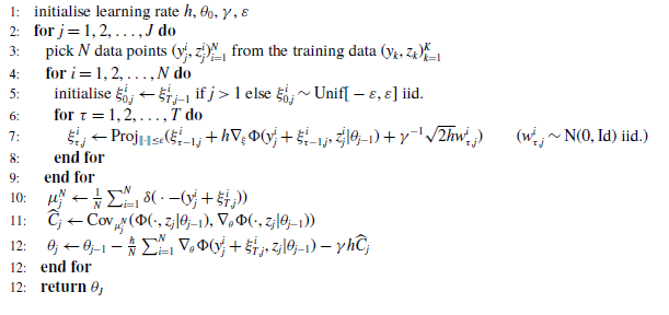
6.2 Discrete Abram with mini-batching
When subsampling in machine learning practice, it is usually advisable to choose mini-batches of data points rather than single data points. Here, we pick a mini-batch
 $\{y_{k'}, z_{k'}\}_{k' \in K'} \subseteq \{y_k, z_k\}_{k=1}^K$
, with
$\{y_{k'}, z_{k'}\}_{k' \in K'} \subseteq \{y_k, z_k\}_{k=1}^K$
, with
 $\#K ' \ll K$
and perform the gradient step with all elements with index in
$\#K ' \ll K$
and perform the gradient step with all elements with index in
 $K'$
rather than a single element in the whole data set
$K'$
rather than a single element in the whole data set
 $\{y_k, z_k\}_{k=1}^K$
. Abram would then require a set of
$\{y_k, z_k\}_{k=1}^K$
. Abram would then require a set of
 $N$
particles for each of the elements in the batch, i.e.
$N$
particles for each of the elements in the batch, i.e.
 $NK'$
particles in total. In practice,
$NK'$
particles in total. In practice,
 $N$
and
$N$
and
 $K'$
are both likely to be large, leading to Abram becoming computationally infeasible. Based on an idea discussed in a different context in [Reference Hanu, Latz and Schillings17], we propose the following method: in every time step
$K'$
are both likely to be large, leading to Abram becoming computationally infeasible. Based on an idea discussed in a different context in [Reference Hanu, Latz and Schillings17], we propose the following method: in every time step
 $j = 1,\ldots, J$
we choose an identical number of particles
$j = 1,\ldots, J$
we choose an identical number of particles
 $(\xi ^{i}_{T,j})_{i=1}^N$
and data points
$(\xi ^{i}_{T,j})_{i=1}^N$
and data points
 $(y^{i}_j,z^{i}_j)_{i=1}^N$
in the mini-batch, i.e.
$(y^{i}_j,z^{i}_j)_{i=1}^N$
in the mini-batch, i.e.
 $\# K' = N$
. Then, we employ the Abram dynamics, but equip each particle
$\# K' = N$
. Then, we employ the Abram dynamics, but equip each particle
 $\xi ^{i}_{T,j}$
with a different data point
$\xi ^{i}_{T,j}$
with a different data point
 $(y^{i}_j,z^{i}_j)$
 $(i = 1,\ldots, N)$
. As opposed to Abram with separate particles per data point, we here compute the sampling covariance throughout all subsampled data points rather than separately for every data point. The resulting dynamics are then only close to (3.1), if we assume that the adversarial attacks for each data point are not too dissimilar of each other. However, the dynamics may also be successful, if this is not the case. We summarise the resulting method in Algorithm2.
$(i = 1,\ldots, N)$
. As opposed to Abram with separate particles per data point, we here compute the sampling covariance throughout all subsampled data points rather than separately for every data point. The resulting dynamics are then only close to (3.1), if we assume that the adversarial attacks for each data point are not too dissimilar of each other. However, the dynamics may also be successful, if this is not the case. We summarise the resulting method in Algorithm2.
6.3 Bayesian attacks
The mechanism used to approximate the Bayesian adversary in Algorithm1 can naturally be used as a Bayesian attack. We propose two different attacks:
-
1. We use the projected Euler–Maruyama method to sample from the Bayesian adversarial distribution
$\pi ^{\gamma, \varepsilon }$
corresponding to an input dataset
$y \in Y$
and model parameter
$\theta ^*$
. We summarise this attack in Algorithm3. -
2. Instead of attacking with a sample from
$\pi ^{\gamma, \varepsilon }$
, we can attack with the mean of said distribution. From Proposition 5.6, we know that the particle system
$(\widehat {\xi }_t)_{t \geq 0}$
that is based on a fixed parameter
$\theta _*$
, is exponentially ergodic. Thus, we approximate the mean of
$\pi ^{\gamma, \varepsilon }$
, by sampling
$(\widehat {\xi }_t)_{t \geq 0}$
using projected Euler–Maruyama and approximate the mean by computing the sample mean throughout the sampling path. We summarise this method in Algorithm4.


Algorithm 3 Bayesian sample attack
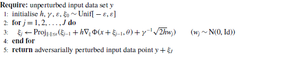
Algorithm 4 Bayesian mean attack

7 Deep learning experiments
We now study the application of Abram in deep learning. The model parameter
 $\theta$
is updated with batch size/number of particles
$\theta$
is updated with batch size/number of particles
 $N$
. For each particle in the ensemble, the perturbation parameter
$N$
. For each particle in the ensemble, the perturbation parameter
 $\xi$
is updated for
$\xi$
is updated for
 $T$
steps. Each experimental run is conducted on a single Nvidia A6000 GPU.
$T$
steps. Each experimental run is conducted on a single Nvidia A6000 GPU.
7.1 MNIST
We test Algorithm1 and Algorithm2 on the classification benchmark data set MNIST [Reference LeCun and Cortes30] against different adversarial attacks and compare the results with the results after an FGSM-based [Reference Wong, Rice and Kolter57] adversarial training. We utilise the Adversarial Robustness Toolbox (ART) for the experiments, see [Reference Nicolae, Sinn, Tran, Buesser, Rawat, Wistuba, Zantedeschi, Baracaldo, Chen, Ludwig, Molloy and Edwards37] for more details. ART is a Python library for adversarial robustness that provides various APIs for defence and attack. We use a neural network with two convolution layers each followed by a max pooling. In Algorithm1, we set
 $\gamma =1, h=\varepsilon, \varepsilon =0.2$
. In Algorithm2, we set
$\gamma =1, h=\varepsilon, \varepsilon =0.2$
. In Algorithm2, we set
 $\gamma =1, h=10\varepsilon, \varepsilon =0.2$
. We observe that setting larger noise scale for the attack during training helps Abram’s final evaluation performance. We train the neural network for 30 epochs (i.e. 30 full iterations through the data set) for each method. The number of particles (and batch size) is
$\gamma =1, h=10\varepsilon, \varepsilon =0.2$
. We observe that setting larger noise scale for the attack during training helps Abram’s final evaluation performance. We train the neural network for 30 epochs (i.e. 30 full iterations through the data set) for each method. The number of particles (and batch size) is
 $N=128$
, and the inner loop is trained for
$N=128$
, and the inner loop is trained for
 $T=10$
times. To better understand how Abram responds to different attacks, we test against six attack methods: PGD [Reference Madry, Makelov, Schmidt, Tsipras and Vladu32], Auto-PGD [Reference Croce and Hein9], Carlini and Wagner [Reference Carlini and Wagner6], Wasserstein Attack [Reference Wong, Schmidt and Kolter56], as well as the Bayesian attacks introduced in this paper – see Algorithms3 and 4. We also test the method’s accuracy in the case of benign (non-attacked) input data. For the Bayesian sample attack and Bayesian mean attack, we set
$T=10$
times. To better understand how Abram responds to different attacks, we test against six attack methods: PGD [Reference Madry, Makelov, Schmidt, Tsipras and Vladu32], Auto-PGD [Reference Croce and Hein9], Carlini and Wagner [Reference Carlini and Wagner6], Wasserstein Attack [Reference Wong, Schmidt and Kolter56], as well as the Bayesian attacks introduced in this paper – see Algorithms3 and 4. We also test the method’s accuracy in the case of benign (non-attacked) input data. For the Bayesian sample attack and Bayesian mean attack, we set
 $\gamma =1000$
. See Table 2 for the comparison. The results are averaged over three random seeds. We observe that Abram performs similarly to FGSM under Wasserstein, Bayesian sample and Bayesian mean attack. FGSM outperforms Abram under Auto-PGD, PGD and Carlini & Wagner attack. We conclude that Abram is as effective as FGSM under certain weaker attacks, but can usually not outperform the conventional FGSM.
$\gamma =1000$
. See Table 2 for the comparison. The results are averaged over three random seeds. We observe that Abram performs similarly to FGSM under Wasserstein, Bayesian sample and Bayesian mean attack. FGSM outperforms Abram under Auto-PGD, PGD and Carlini & Wagner attack. We conclude that Abram is as effective as FGSM under certain weaker attacks, but can usually not outperform the conventional FGSM.
Table 2. Comparison of test accuracy (%) on MNIST with different adversarial attack after Abram, mini-batching Abram, and FGSM [Reference Wong, Rice and Kolter57] adversarial training

Another observation is that mini-batching Abram outperforms Abram significantly. Recall that in Abram we have used
 $128$
particles for each data point which can be viewed as SGD with batch size
$128$
particles for each data point which can be viewed as SGD with batch size
 $1$
, whereas the mini-batching Abram is similar to the mini-batching SGD. Mini-batching Abram has the freedom to set the batch size which helps to reduce the variance in the stochastic optimisation and, thus, gives more stable results. In particular, with mini-batching Abram, gradients are approximated by multiple data points instead of one data point which is the case in Abram. Having a larger batch size also increases computation efficiency by doing matrix multiplication on GPUs, which is important in modern machine learning applications as the datasets can be expected to be large.
$1$
, whereas the mini-batching Abram is similar to the mini-batching SGD. Mini-batching Abram has the freedom to set the batch size which helps to reduce the variance in the stochastic optimisation and, thus, gives more stable results. In particular, with mini-batching Abram, gradients are approximated by multiple data points instead of one data point which is the case in Abram. Having a larger batch size also increases computation efficiency by doing matrix multiplication on GPUs, which is important in modern machine learning applications as the datasets can be expected to be large.
7.2 CIFAR10
Similarly, we test Algorithm2 on the classification benchmark dataset CIFAR10 [Reference Krizhevsky23] by utilising ART. The dataset is pre-processed by random crop and random horizontal flip following [Reference Krizhevsky23] for data augmentation. The neural network uses the Pre-act ResNet-18 [Reference He, Zhang, Ren and Sun18] architecture. For Abram, we set
 $\gamma =1, h=\varepsilon, \varepsilon =16/255$
. Similar as in the MNIST experiments, practically we find that setting larger noise scale for attack in training Abram helps to obtain a better final evaluation performance. The batch size
$\gamma =1, h=\varepsilon, \varepsilon =16/255$
. Similar as in the MNIST experiments, practically we find that setting larger noise scale for attack in training Abram helps to obtain a better final evaluation performance. The batch size
 $N=128$
and the inner loop is simulated for
$N=128$
and the inner loop is simulated for
 $T=10$
times. We train both mini-batching Abram and FGSM for 30 epochs. Due to its worse performance for MNIST and the large size of CIFAR10, we have not used the non-mini-batching version of Abram in this second problem. For the Bayesian sample attack and the Bayesian mean attack, we set
$T=10$
times. We train both mini-batching Abram and FGSM for 30 epochs. Due to its worse performance for MNIST and the large size of CIFAR10, we have not used the non-mini-batching version of Abram in this second problem. For the Bayesian sample attack and the Bayesian mean attack, we set
 $\gamma =1000$
. We present the results in Table 3. There, we observe that mini-batching Abram outperforms FGSM under Wasserstein and the Bayesian attacks, but not in any of the other cases.
$\gamma =1000$
. We present the results in Table 3. There, we observe that mini-batching Abram outperforms FGSM under Wasserstein and the Bayesian attacks, but not in any of the other cases.
Table 3. Comparison of test accuracy (%) on CIFAR10 with different adversarial attack after mini-batching Abram and FGSM [Reference Wong, Rice and Kolter57] adversarial training

8 Conclusions
We have introduced the Bayesian adversarial robustness problem. This problem can be interpreted as either a relaxation of the usual minmax problem in adversarial learning or as learning methodology that is able to counter Bayesian adversarial attacks. To solve the Bayesian adversarial robustness problem, we introduce Abram – the Adversarially Bayesian Particle Sampler. Under restrictive assumptions, we prove that Abram approximates a McKean–Vlasov SDE and that this McKean–Vlasov SDE is able to find the minimiser of certain (simple) Bayesian adversarial robustness problems. Thus, at least for a certain class of problems, we give a mathematical justification for the use of Abram. We propose two ways to discretise Abram: a direct Euler–Maruyama discretisation of the Abram dynamics and an alternative method that is more suitable when training with respect to large data sets. We apply Abram in two deep learning problems. There we see that Abram can effectively prevent certain adversarial attacks (especially Bayesian attacks), but is overall not as strong as classical optimisation-based heuristics.
Competing interests
The authors declare none.


 Open access