


1 Introduction and motivations
The interaction between monochromatic, propagating, linear electromagnetic waves with obstructing boundaries is key to many topical scattering problems which arise in modern applications of wave theory. In order to understand these phenomena, entire theories such as Keller’s geometric theory of diffraction [Reference Keller7, Reference Keller8], relevant in the high-frequency domain, have been developed and applied with success (by James [Reference James6], for example).
Friedlander & Keller [Reference Friedlander and Keller5] extended the idea of using ray theory to solve the scalar Helmholtz equation. One aim of this paper is to develop an equivalent method for Maxwell’s equations of electromagnetism for time-harmonic waves in the high-frequency limit. As per Friedlander & Keller, there are specific applications for which classic ray theory must be amended in order to accommodate them; this amendment comes in the Wentzel Kramers Brillouin-Jeffreys (WKBJ)-type expansion of the assumed solutions.
The second aim of this paper is to provide, in full detail, a set of canonical applications of waves radiating from boundaries that conform to a wave-front. The theory presented in this paper will then be used to determine the phase structure and the leading-order amplitude solutions to these specific problems.
As Maxwell’s equations can, in certain circumstances, be reduced to satisfy two decoupled vectorial Helmholtz equations (one each for the electric and magnetic fields), it makes sense that motivation for the studies conducted here is rooted in the literature of the study of the scalar Helmholtz equation. In fact, Keller [Reference Keller, Lewis and Seckler10] even considered the individual components of the electric vector and said they must each satisfy their own Helmholtz equation. This idea was later used by Radjen et al. [Reference Radjen, Gradoni and Tew15].
The scalar Helmholtz equation is
 \begin{eqnarray}\left(\nabla^2+k^2\right)\!\phi&=&0.\end{eqnarray}
Many authors attempted to solve this in the high-frequency limit
 $k\rightarrow\infty$
. Keller [Reference Keller, Lewis and Seckler10] gave an explanation of the method used and then provided some practical applications for it. Similarly, Luneburg [Reference Luneburg12] considered an identical asymptotic expansion for components of Maxwell’s equations. The idea is to take the asymptotic solution
$k\rightarrow\infty$
. Keller [Reference Keller, Lewis and Seckler10] gave an explanation of the method used and then provided some practical applications for it. Similarly, Luneburg [Reference Luneburg12] considered an identical asymptotic expansion for components of Maxwell’s equations. The idea is to take the asymptotic solution
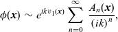 \begin{eqnarray}\phi(\boldsymbol{{x}})&\sim&e^{ikv_1(\boldsymbol{{x}})}\sum_{n=0}^\infty\;\frac{A_n(\boldsymbol{{x}})}{\left(ik\right)^n},\end{eqnarray}
in order to derive field equations for the exponential ‘phase’ term, the leading-order amplitude function
 $A_0$
, as well as higher-order corrections. Substitution of ansatz (1.2) into the Helmholtz equation (1.1) and comparing the different values of k gives
$A_0$
, as well as higher-order corrections. Substitution of ansatz (1.2) into the Helmholtz equation (1.1) and comparing the different values of k gives
 \begin{eqnarray}\boldsymbol{\nabla}v_1\boldsymbol{\cdot}\boldsymbol{\nabla}v_1&=&1,\end{eqnarray}
 \begin{eqnarray}2\!\left(\boldsymbol{\nabla}A_n\boldsymbol{\cdot}\boldsymbol{\nabla}v_1\right)+A_n\nabla^2v_1+\nabla^2A_{n-1}&=&0,\end{eqnarray}
in which
 $A_{-1}\equiv 0$
is understood, allowing the transport equation for the leading-order term to be incorporated with those for the higher-order corrections. Equation (1.3) is the eikonal equation of geometric optics. At leading order, this completely decouples from the amplitude functions. Equation (1.4) is a recursive set of equations for the amplitude functions. In order to provide solutions to these equations, Keller et al. adopted a curvilinear ‘ray’ coordinate system, which used parameters
$A_{-1}\equiv 0$
is understood, allowing the transport equation for the leading-order term to be incorporated with those for the higher-order corrections. Equation (1.3) is the eikonal equation of geometric optics. At leading order, this completely decouples from the amplitude functions. Equation (1.4) is a recursive set of equations for the amplitude functions. In order to provide solutions to these equations, Keller et al. adopted a curvilinear ‘ray’ coordinate system, which used parameters
 $\boldsymbol{{s}}$
to describe a wave-front, and a parameter
$\boldsymbol{{s}}$
to describe a wave-front, and a parameter
 $\tau$
to denote length along an individual ray emitting from that wave-front. Solutions were then found for the amplitude functions in terms of integrals
$\tau$
to denote length along an individual ray emitting from that wave-front. Solutions were then found for the amplitude functions in terms of integrals
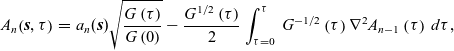 \begin{eqnarray}A_n\!\left(\boldsymbol{{s}},\tau\right)&=&a_n(\boldsymbol{{s}})\sqrt{\frac{G\left(\tau\right)}{G\left(0\right)}}-\frac{G^{1/2}\left(\tau\right)}{2}\int_{\tau=0}^\tau\;G^{-1/2}\left(\tau\right)\nabla^2A_{n-1}\left(\tau\right)\;d\tau,\end{eqnarray}
where
 $a_n$
is the value of
$a_n$
is the value of
 $A_n$
along the wave-front and
$A_n$
along the wave-front and
 $G\left(\tau\right)$
denoting the Gaussian curvature of the wave-front. These geometric results will be significant in the derivation of the electromagnetic equivalent. Keller et al. then went on to analyse these equations for specified wave-fronts and then to use these to determine the dynamics of the scattered field when incident rays encountered certain geometries.
$G\left(\tau\right)$
denoting the Gaussian curvature of the wave-front. These geometric results will be significant in the derivation of the electromagnetic equivalent. Keller et al. then went on to analyse these equations for specified wave-fronts and then to use these to determine the dynamics of the scattered field when incident rays encountered certain geometries.
Levy & Keller [Reference Levy and Keller11] took this further and found a ‘ray solution’ to the eikonal equation (1.3)
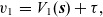 \begin{eqnarray}v_1&=&V_1(\boldsymbol{{s}})+\tau,\end{eqnarray}
where
 $V_1(\boldsymbol{{s}})$
is the imposed boundary data (i.e.
$V_1(\boldsymbol{{s}})$
is the imposed boundary data (i.e.
 $V_1(\boldsymbol{{s}})=v_1\!\left(\boldsymbol{{s}},0\right)$
). The important result here was that the rays are, in fact, straight lines. By using an energy conservation principle, they examined the flux through a cross-sectional area of a tube of rays (which they note as being simple owing to the rays being straight lines), and they found that the solution to the Helmholtz equation (1.1), correct to leading order, is
$V_1(\boldsymbol{{s}})=v_1\!\left(\boldsymbol{{s}},0\right)$
). The important result here was that the rays are, in fact, straight lines. By using an energy conservation principle, they examined the flux through a cross-sectional area of a tube of rays (which they note as being simple owing to the rays being straight lines), and they found that the solution to the Helmholtz equation (1.1), correct to leading order, is
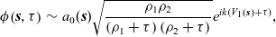 \begin{eqnarray}\phi\!\left(\boldsymbol{{s}},\tau\right)&\sim&a_0(\boldsymbol{{s}})\sqrt{\frac{\rho_1\rho_2}{\left(\rho_1+\tau\right)\left(\rho_2+\tau\right)}}e^{ik\left(V_1(\boldsymbol{{s}})+\tau\right)},\end{eqnarray}
where
 $\rho_1$
and
$\rho_1$
and
 $\rho_2$
are the radii of curvature of the wave-front in the two principal directions. Later in that paper, the authors used this result to obtain solutions to electromagnetic problems by compartmentalising the electric field vector into three individual scalar components, each of which satisfies their own (scalar) Helmholtz equation. Of course, this is an argument which only holds true in a Cartesian frame and is not true generally.
$\rho_2$
are the radii of curvature of the wave-front in the two principal directions. Later in that paper, the authors used this result to obtain solutions to electromagnetic problems by compartmentalising the electric field vector into three individual scalar components, each of which satisfies their own (scalar) Helmholtz equation. Of course, this is an argument which only holds true in a Cartesian frame and is not true generally.
The vectorial form of ansatz (1.2) for the electric and magnetic fields was taken and applied by Keller & Lewis [Reference Keller and Lewis9] to obtain field equations for the exponent term and the amplitudes of the two electromagnetic fields. They did not solve these equations (or even decouple the two fields). Later, Molinet et al. [Reference Molinet, Andronov and Bouche13] used Keller’s geometric theory of diffraction to provide the leading-order solution to the electric field.
It quickly became apparent that modifications to this ‘classical’ approach were required. Friedlander & Keller [Reference Friedlander and Keller5] mentioned several diffraction problems which have additional exponent terms proportional to a power of the wave-number k. Although some specific research had been conducted on some of these problems ([Reference Bremmer2] and [Reference Friedlander4]), there was not any widely available theory. Therefore, they sought to modify this ray ansatz to accommodate a broader range of these problems and took the solution to the Helmholtz equation as
 \begin{eqnarray}\phi(\boldsymbol{{x}})&\sim&e^{ikv_1+ik^{\alpha}v_2}\sum_{n=0}^\infty\;\frac{A_n(\boldsymbol{{x}})}{k^{\lambda_n}},\end{eqnarray}
in which
 $\lambda_1<\lambda_2<\cdots$
were to be determined. Their analysis showed that if
$\lambda_1<\lambda_2<\cdots$
were to be determined. Their analysis showed that if
 $\displaystyle{\alpha>\frac{1}{2}}$
, then the additional exponent term
$\displaystyle{\alpha>\frac{1}{2}}$
, then the additional exponent term
 $v_2$
was necessarily constant. In that case, the
$v_2$
was necessarily constant. In that case, the
 $\exp\left(ik^{\alpha}v_2\right)$
term was amalgamable into the amplitude profile, essentially reducing ansatz (1.8) to a slightly altered but fundamentally unchanged form of ansatz (1.2). If
$\exp\left(ik^{\alpha}v_2\right)$
term was amalgamable into the amplitude profile, essentially reducing ansatz (1.8) to a slightly altered but fundamentally unchanged form of ansatz (1.2). If
 $\alpha\le 0$
, then the expansion of the
$\alpha\le 0$
, then the expansion of the
 $\exp\left(ik^{\alpha}v_2\right)$
term proceeds in decreasing powers of k. Again, those terms are amalgamable into the amplitude profile, so a choice of
$\exp\left(ik^{\alpha}v_2\right)$
term proceeds in decreasing powers of k. Again, those terms are amalgamable into the amplitude profile, so a choice of
 $\alpha$
in that range would also reduce ansatz (1.8) to a fundamentally unchanged form of ansatz (1.2). Therefore, the authors demonstrated that the additional exponent term at
$\alpha$
in that range would also reduce ansatz (1.8) to a fundamentally unchanged form of ansatz (1.2). Therefore, the authors demonstrated that the additional exponent term at
 $O\!\left(k^{\alpha}\right)$
is variable if and only if
$O\!\left(k^{\alpha}\right)$
is variable if and only if
 $\alpha$
has a value in the range
$\alpha$
has a value in the range
 $0<\alpha\le \displaystyle{\frac{1}{2}}$
. With this range fixed, they found that
$0<\alpha\le \displaystyle{\frac{1}{2}}$
. With this range fixed, they found that
 $v_1$
still obeyed the eikonal equation (1.3) . They also found that the field equation for
$v_1$
still obeyed the eikonal equation (1.3) . They also found that the field equation for
 $v_2$
is
$v_2$
is
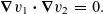 \begin{eqnarray}\boldsymbol{\nabla}v_1\boldsymbol{\cdot}\boldsymbol{\nabla}v_2&=&0.\end{eqnarray}
A little further into their investigation, they determined that there were two field equations for the leading-order amplitude:
 \begin{eqnarray}2\!\left(\boldsymbol{\nabla}A_0\boldsymbol{\cdot}\boldsymbol{\nabla}v_1\right)+A_0\nabla^2v_1&=&0,\ \ \mbox{for}\ \ 0<\alpha<\frac{1}{2},\end{eqnarray}
 \begin{eqnarray}2\!\left(\boldsymbol{\nabla}A_0\boldsymbol{\cdot}\boldsymbol{\nabla}v_1\right)+A_0\!\left(\nabla^2v_1+i\left(\boldsymbol{\nabla}v_2\boldsymbol{\cdot}\boldsymbol{\nabla}v_2\right)\right)&=&0,\ \ \mbox{for}\ \ \alpha=\frac{1}{2}.\end{eqnarray}
Equation (1.10) is exactly the same as equation (1.4) . However, if
 $\displaystyle{\alpha=\frac{1}{2}}$
, then there is an additional term in the transport equation, and it is this change that they originally sought. Additionally, Engineer et al. [Reference Engineer, King and Tew3] also showed, by presenting geometric arguments, that
$\displaystyle{\alpha=\frac{1}{2}}$
, then there is an additional term in the transport equation, and it is this change that they originally sought. Additionally, Engineer et al. [Reference Engineer, King and Tew3] also showed, by presenting geometric arguments, that
 $k^{1/2}$
is an isolated case of exceptional importance. Thus, the value of
$k^{1/2}$
is an isolated case of exceptional importance. Thus, the value of
 $\displaystyle{\alpha=\frac{1}{2}}$
is canonical as it is the only value of
$\displaystyle{\alpha=\frac{1}{2}}$
is canonical as it is the only value of
 $\alpha$
for which precisely one additional exponent term leads to a modified transport equation at leading order.
$\alpha$
for which precisely one additional exponent term leads to a modified transport equation at leading order.
Tew [Reference Tew17] aimed to solve a new class of two-dimensional scattering problems which were the scattering of an acoustic wave upon a ‘perturbed’ boundary. These perturbed boundaries were acoustically soft and of the form
 $\boldsymbol{{x}}_0(s)+k^{-1/2}\boldsymbol{\hat{x}}_0(s)$
, where
$\boldsymbol{{x}}_0(s)+k^{-1/2}\boldsymbol{\hat{x}}_0(s)$
, where
 $\boldsymbol{{x}}_0$
was a boundary of arbitrary
$\boldsymbol{{x}}_0$
was a boundary of arbitrary
 $O\!\left(1\right)$
curvature parametrised by arc-length s and on which small scale undulations were imposed and given by
$O\!\left(1\right)$
curvature parametrised by arc-length s and on which small scale undulations were imposed and given by
 $\boldsymbol{\hat{x}}_0$
. It followed that when a ‘classic’ wave (i.e. one exponent term) appearing at
$\boldsymbol{\hat{x}}_0$
. It followed that when a ‘classic’ wave (i.e. one exponent term) appearing at
 $O\!\left(k\right)$
encountered this boundary, then there would be an additional term appearing at
$O\!\left(k\right)$
encountered this boundary, then there would be an additional term appearing at
 $O\!\left(k^{1/2}\right)$
in the exponent. Therefore, the scattered field must then take the form of a Friedlander–Keller ray expansion (with
$O\!\left(k^{1/2}\right)$
in the exponent. Therefore, the scattered field must then take the form of a Friedlander–Keller ray expansion (with
 $\displaystyle{\alpha=\frac{1}{2}}$
). Through this research, Tew obtained the solutions to equations (1.9) and (1.11):
$\displaystyle{\alpha=\frac{1}{2}}$
). Through this research, Tew obtained the solutions to equations (1.9) and (1.11):
 \begin{eqnarray}v_2(s,\tau)&=&V_2(s),\end{eqnarray}
 \begin{eqnarray}A_0(s,\tau)&=&a_0(s)\sqrt{\frac{a_2(s)}{a(s)+\tau}}\exp\left(-\frac{ib_2(s)\tau}{2a_2\!\left(a_2(s)+\tau\right)}\right),\end{eqnarray}
where
 $a_2$
and
$a_2$
and
 $b_2$
are known functions which are specific to the two-dimensional boundaries (hence the subscription ‘2’) and are defined as
$b_2$
are known functions which are specific to the two-dimensional boundaries (hence the subscription ‘2’) and are defined as
 \begin{eqnarray}a_2(s)&=&\frac{q_0(s)x_0^{\prime}(s)-p_0(s)y_0^{\prime}(s)}{q_0(s)p_0^{\prime}(s)-p_0(s)q_0^{\prime}(s)}\nonumber\\[4pt]b_2(s)&=&\left(\frac{V_2^{\prime}(s)}{q_0(s)p_0^{\prime}(s)-p_0(s)q_0^{\prime}(s)}\right)^2,\end{eqnarray}
in which
 $p_0$
and
$p_0$
and
 $q_0$
specify the ray directions, and their ratio
$q_0$
specify the ray directions, and their ratio
 $\displaystyle{\frac{q_0}{p_0}}$
describes the gradient of the associated ray. The boundary
$\displaystyle{\frac{q_0}{p_0}}$
describes the gradient of the associated ray. The boundary
 $\boldsymbol{{x}}_0(s)$
has components
$\boldsymbol{{x}}_0(s)$
has components
 $x_0(s)$
and
$x_0(s)$
and
 $y_0(s)$
; these are relative to a traditional Cartesian frame.
$y_0(s)$
; these are relative to a traditional Cartesian frame.
Many topical areas of diffraction theory relate to creeping waves which include additional exponent terms proportional to
 $k^{1/3}$
and are discussed at length by various authors ([Reference Engineer, King and Tew3], [Reference Molinet, Andronov and Bouche13], and [Reference Tew, Chapman, King, Ockendon, Smith and Zafarullah19], for example). This particular exponent term correlates to assigning the value
$k^{1/3}$
and are discussed at length by various authors ([Reference Engineer, King and Tew3], [Reference Molinet, Andronov and Bouche13], and [Reference Tew, Chapman, King, Ockendon, Smith and Zafarullah19], for example). This particular exponent term correlates to assigning the value
 $\displaystyle{\alpha=\frac{1}{3}}$
in the Friedlander–Keller ansatz (1.8). Andronov & Bouche [Reference Molinet, Andronov and Bouche13], for example, aimed to provide the leading-order and first-order correction solutions to the creeping rays arising from the diffraction of an electromagnetic wave incident upon a smooth convex object. Keller [Reference Keller7, Reference Keller8] demonstrated that diffracted rays act as ordinary rays when far enough away from the diffracting object. Thus, Andronov & Bouche [Reference Molinet, Andronov and Bouche13] assumed a solution for the electric and magnetic fields in the form of Friedlander–Keller ansatz (1.8) with
$\displaystyle{\alpha=\frac{1}{3}}$
in the Friedlander–Keller ansatz (1.8). Andronov & Bouche [Reference Molinet, Andronov and Bouche13], for example, aimed to provide the leading-order and first-order correction solutions to the creeping rays arising from the diffraction of an electromagnetic wave incident upon a smooth convex object. Keller [Reference Keller7, Reference Keller8] demonstrated that diffracted rays act as ordinary rays when far enough away from the diffracting object. Thus, Andronov & Bouche [Reference Molinet, Andronov and Bouche13] assumed a solution for the electric and magnetic fields in the form of Friedlander–Keller ansatz (1.8) with
 $\displaystyle{\alpha=\frac{1}{3}}$
for the far-field solution and matched this asymptotically to the solution in the boundary layer.
$\displaystyle{\alpha=\frac{1}{3}}$
for the far-field solution and matched this asymptotically to the solution in the boundary layer.
In general, the value of
 $\displaystyle{\alpha=\frac{1}{3}}$
in ansatz (1.8) does not lead to a different transport equation than the classic case, as demonstrated by Friedlander & Keller [Reference Friedlander and Keller5]. The value of
$\displaystyle{\alpha=\frac{1}{3}}$
in ansatz (1.8) does not lead to a different transport equation than the classic case, as demonstrated by Friedlander & Keller [Reference Friedlander and Keller5]. The value of
 $\displaystyle{\alpha=\frac{1}{2}}$
is canonical for the reasons cited above. However, this value of
$\displaystyle{\alpha=\frac{1}{2}}$
is canonical for the reasons cited above. However, this value of
 $\alpha$
is a direct consequence of including only one additional term in the exponent (that appearing at
$\alpha$
is a direct consequence of including only one additional term in the exponent (that appearing at
 $O\!\left(k^{\alpha}\right)$
). It is possible to include a further exponent term in ansatz (1.8), say at
$O\!\left(k^{\alpha}\right)$
). It is possible to include a further exponent term in ansatz (1.8), say at
 $O\!\left(k^{\beta}\right)$
, and proceeding in a derivation akin to that performed by Friedlander & Keller [Reference Friedlander and Keller5]. Doing so yields that the two canonical values of
$O\!\left(k^{\beta}\right)$
, and proceeding in a derivation akin to that performed by Friedlander & Keller [Reference Friedlander and Keller5]. Doing so yields that the two canonical values of
 $\alpha$
and
$\alpha$
and
 $\beta$
would be
$\beta$
would be
 $\displaystyle{\alpha=\frac{1}{3}}$
and
$\displaystyle{\alpha=\frac{1}{3}}$
and
 $\displaystyle{\beta=\frac{2}{3}}$
(without loss of generality). This approach was generalised by Tew [Reference Tew18], who developed the generalised Friedlander–Keller ray expansion of fractional order. The idea is to assume an arbitrary number of exponent terms in decreasing fractional powers of k and include a suitably altered WKBJ expansion of the amplitude. Thus, the solution of Helmholtz equation (1.1)
$\displaystyle{\beta=\frac{2}{3}}$
(without loss of generality). This approach was generalised by Tew [Reference Tew18], who developed the generalised Friedlander–Keller ray expansion of fractional order. The idea is to assume an arbitrary number of exponent terms in decreasing fractional powers of k and include a suitably altered WKBJ expansion of the amplitude. Thus, the solution of Helmholtz equation (1.1)
 $\phi$
has the expansion
$\phi$
has the expansion
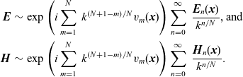
 \begin{eqnarray}\phi(\boldsymbol{{x}})&\sim&\exp\!\left(i\sum_{m=1}^N\;k^{\left(N+1-m\right)/N}v_m(\boldsymbol{{x}})\right)\sum_{n=0}^\infty\;\frac{A_n(\boldsymbol{{x}})}{k^{n/N}},\end{eqnarray}
for an arbitrary positive integer N (setting
 $N=2$
essentially repeating the work of Friedlander & Keller [Reference Friedlander and Keller5]).
$N=2$
essentially repeating the work of Friedlander & Keller [Reference Friedlander and Keller5]).
Without repeating the derivation performed by Tew [Reference Tew18] in full, the main results were that
 $v_1$
(which appears at leading-order k in the exponent) still obeys the eikonal equation (1.3), and the remaining phase terms
$v_1$
(which appears at leading-order k in the exponent) still obeys the eikonal equation (1.3), and the remaining phase terms
 $v_2,\cdots,v_N$
obey the system of partial differential equations
$v_2,\cdots,v_N$
obey the system of partial differential equations
 \begin{eqnarray}\sum_{j=0}^n\!\left(\boldsymbol{\nabla}v_{n+1-j}\boldsymbol{\cdot}\boldsymbol{\nabla}v_{j+1}\right)&=&0,\ \ \mbox{for}\ \ n=1,2,\cdots,N-1.\end{eqnarray}
The additional
 $N-1$
exponent terms in Tew’s ansatz (1.15) gave rise to a further set of terms appearing in the transport equation, all of which have an i coefficient (which is expected as they come from the exponent). The modified transport equation being
$N-1$
exponent terms in Tew’s ansatz (1.15) gave rise to a further set of terms appearing in the transport equation, all of which have an i coefficient (which is expected as they come from the exponent). The modified transport equation being
 \begin{align}&\sum_{n=1}^N\left[2\!\left(\boldsymbol{\nabla}v_{N+1-n}\boldsymbol{\cdot}\boldsymbol{\nabla}A_{n+q}\right)+\nabla^2v_{N+1-n}A_{n+q}\right]\nonumber\\&\quad +iA_{N+q}\sum_{n=2}^N\left(\boldsymbol{\nabla}v_{N+2-n}\boldsymbol{\cdot}\boldsymbol{\nabla}v_n\right)+i\sum_{n=3}^N\left[A_{N+2+q-n}\sum_{j=n}^N\left(\boldsymbol{\nabla}v_{N+m-j}\boldsymbol{\cdot}\boldsymbol{\nabla}v_j\right)\right]\nonumber\\&\quad -i\nabla^2A_q=0,\end{align}
where
 $A_{-i}\equiv 0\;\left(i=1,2,\cdots,N\right)$
is understood.
$A_{-i}\equiv 0\;\left(i=1,2,\cdots,N\right)$
is understood.
Radjen et al. [Reference Radjen, Gradoni and Tew15] extended the work of Tew [Reference Tew17] by considering boundaries of the same profile but were penetrable rather than acoustically soft. Beyond that boundary was a different homogeneous medium supporting Helmholtz equation (1.1) with
 $k\rightarrow k\gamma^{-1}$
, where
$k\rightarrow k\gamma^{-1}$
, where
 $\gamma^{-1}$
(the refractive index in optical terms) is an
$\gamma^{-1}$
(the refractive index in optical terms) is an
 $O\!\left(1\right)$
constant describing the ratio of the wave-speeds of the two media. Those conditions for
$O\!\left(1\right)$
constant describing the ratio of the wave-speeds of the two media. Those conditions for
 $\gamma$
did not significantly change the theory used. One main point in that paper was the attempt to obtain asymptotic solutions to Maxwell’s equations when an electric field was incident upon this class of boundary. However, as those were two-dimensional problems, an argument was made that the electric field could be scalarised by using the Maxwell equation
$\gamma$
did not significantly change the theory used. One main point in that paper was the attempt to obtain asymptotic solutions to Maxwell’s equations when an electric field was incident upon this class of boundary. However, as those were two-dimensional problems, an argument was made that the electric field could be scalarised by using the Maxwell equation
 $\left(\boldsymbol{\nabla}\boldsymbol{\cdot}\boldsymbol{{E}}\right)=0$
, in standard notation, which, to leading order, gives that
$\left(\boldsymbol{\nabla}\boldsymbol{\cdot}\boldsymbol{{E}}\right)=0$
, in standard notation, which, to leading order, gives that
 \begin{eqnarray}\boldsymbol{{E}}&\sim&E_0\left[-\frac{\partial v_1}{\partial y},\frac{\partial v_1}{\partial x}\right]+O\!\left(k^{-1/2}\right),\end{eqnarray}
for a single scalar unknown variable
 $E_0$
, which satisfies the Helmholtz equation (1.1) inside the boundary (and another Helmholtz equation outside).
$E_0$
, which satisfies the Helmholtz equation (1.1) inside the boundary (and another Helmholtz equation outside).
As stated at the outset, this paper aims to derive a generalised Friedlander–Keller ray expansion for Maxwell’s equations of electromagnetism, in the style of Friedlander & Keller [Reference Friedlander and Keller5] and Tew [Reference Tew18]. This derivation considers Maxwell’s equations in complete vectorial form. Furthermore, it does not assign an initial coordinate system, allowing the results to have freedom of generality. This work complements Radjen et al. [Reference Radjen, Gradoni and Tew15], who restricted their attention to a two-dimensional Cartesian frame, allowing them to reduce Maxwell’s equations to a scalar Helmholtz equation. Although many authors have studied the scalar and vectorial Helmholtz equations geometrically by wave-front data ([Reference Engineer, King and Tew3, Reference Keller and Lewis9, Reference Keller, Lewis and Seckler10, Reference Levy and Keller11, Reference Molinet, Andronov and Bouche13], and others), this investigation will adopt a partial differential equation approach. The key benefit of doing so is to obtain solutions that are widely applicable to modern wave scattering problems, such as the diffraction theory cited above.
2 Generalised Friedlander–Keller ray expansions of Maxwell’s equations
As mentioned from the outset, the aim here is to determine asymptotic solutions to Maxwell’s equations. As presented in standard by form by many authors ([Reference James6, Reference Keller and Lewis9, Reference Molinet, Andronov and Bouche13, Reference Rothwell and Cloud16], for examples), an electric field
 $\boldsymbol{{E}}$
and a magnetic field
$\boldsymbol{{E}}$
and a magnetic field
 $\boldsymbol{{H}}$
in a charge-free vacuum satisfy
$\boldsymbol{{H}}$
in a charge-free vacuum satisfy
 \begin{eqnarray}\left(\boldsymbol{\nabla}{\times}\boldsymbol{{E}}\right)=ik\sqrt{\frac{\mu}{\epsilon}}\boldsymbol{{H}}&\mbox{ and }&\left(\boldsymbol{\nabla}{\times}\boldsymbol{{H}}\right)=-ik\sqrt{\frac{\epsilon}{\mu}}\boldsymbol{{E}},\end{eqnarray}
 \begin{eqnarray}\boldsymbol{\nabla}\boldsymbol{\cdot}\boldsymbol{{E}}=0&\mbox{ and }&\boldsymbol{\nabla}\boldsymbol{\cdot}\boldsymbol{{H}}=0,\end{eqnarray}
in which k is the large wave-number. Here, a time-harmonic,
 $e^{-i\omega t}$
, form is assumed yet suppressed and is related to the wave-number by
$e^{-i\omega t}$
, form is assumed yet suppressed and is related to the wave-number by
 $k=\omega\sqrt{\epsilon\mu}$
. The scalar quantities
$k=\omega\sqrt{\epsilon\mu}$
. The scalar quantities
 $\epsilon$
and
$\epsilon$
and
 $\mu$
represent the permittivity and permeability of the medium and are both
$\mu$
represent the permittivity and permeability of the medium and are both
 $O\!\left(1\right)$
constants – they relate to the speed of light by
$O\!\left(1\right)$
constants – they relate to the speed of light by
 $\displaystyle{c=\frac{1}{\sqrt{\epsilon\mu}}}$
, but they will be kept separate here for the sake of generalisation. Although it is possible to consider a pair of decoupled vectorial forms of Helmholtz equation (1.1), the two fields will deliberately remain coupled until the end of the derivation, which is merely for computational convenience.
$\displaystyle{c=\frac{1}{\sqrt{\epsilon\mu}}}$
, but they will be kept separate here for the sake of generalisation. Although it is possible to consider a pair of decoupled vectorial forms of Helmholtz equation (1.1), the two fields will deliberately remain coupled until the end of the derivation, which is merely for computational convenience.
The classical approach, as presented by Keller & Lewis [Reference Keller and Lewis9] and Molinet et al. [Reference Molinet, Andronov and Bouche13], seeks solutions to Maxwell’s equations (2.1) and (2.2) in the singularly perturbed, high-frequency limit
 $k\rightarrow\infty$
with the WKBJ form
$k\rightarrow\infty$
with the WKBJ form
 \begin{eqnarray}\boldsymbol{{E}}(\boldsymbol{{x}})\sim e^{ikv_1(\boldsymbol{{x}})}\sum_{n=0}^\infty\;\frac{\boldsymbol{{E}}_n(\boldsymbol{{x}})}{\left(ik\right)^n}&\mbox{ and }&\boldsymbol{{H}}(\boldsymbol{{x}})\sim e^{ikv_1(\boldsymbol{{x}})}\sum_{n=0}^\infty\;\frac{\boldsymbol{{H}}_n(\boldsymbol{{x}})}{\left(ik\right)^n}.\end{eqnarray}
Without diving too deep into the details of the derivation (as this is given below), substituting these ansätze into Maxwell’s equations (2.1) and (2.2) quickly gives that
 $v_1$
obeys the eikonal equation (1.3) and, after a little algebraic patience, the transport equations for the
$v_1$
obeys the eikonal equation (1.3) and, after a little algebraic patience, the transport equations for the
 $\boldsymbol{{E}}_n$
and
$\boldsymbol{{E}}_n$
and
 $\boldsymbol{{H}}_n$
fields decouple and are given as
$\boldsymbol{{H}}_n$
fields decouple and are given as
 \begin{eqnarray}2\!\left(\boldsymbol{\nabla}v_1\boldsymbol{\cdot}\boldsymbol{\nabla}\right)\boldsymbol{{E}}_n+\nabla^2v_1\boldsymbol{{E}}_n&=&-\nabla^2\boldsymbol{{E}}_{n-1},\end{eqnarray}
 \begin{eqnarray}2\!\left(\boldsymbol{\nabla}v_1\boldsymbol{\cdot}\boldsymbol{\nabla}\right)\boldsymbol{{H}}_n+\nabla^2v_1\boldsymbol{{H}}_n&=&-\nabla^2\boldsymbol{{H}}_{n-1}.\end{eqnarray}
Note how the eikonal equation (1.3) decouples entirely from the electric and magnetic fields and then feeds into those latter equations. Therefore, the eikonal equation needs solving first by using Charpit’s method of characteristics as presented by Zauderer [Reference Zauderer20] and Ockendon et al. [Reference Ockendon, Howison, Lacey and Movchan14]. Detailed solutions are presented elsewhere by Tew [Reference Tew17, Reference Tew18] and Radjen et al. [Reference Radjen, Gradoni and Tew15]; those are directly relevant to the purposes of this paper. Introducing characteristic curves
 $\Gamma\!\left(\tau\right)$
as the rays and defined as
$\Gamma\!\left(\tau\right)$
as the rays and defined as
 $\displaystyle{\frac{d\boldsymbol{{x}}}{d\tau}=\boldsymbol{\nabla}v_1}$
which emanate from a generic boundary
$\displaystyle{\frac{d\boldsymbol{{x}}}{d\tau}=\boldsymbol{\nabla}v_1}$
which emanate from a generic boundary
 $\boldsymbol{{x}}_0$
then, along the ray
$\boldsymbol{{x}}_0$
then, along the ray
 $\Gamma$
, several results hold. Firstly, the eikonal equation (1.3) becomes
$\Gamma$
, several results hold. Firstly, the eikonal equation (1.3) becomes
 $\displaystyle{\frac{d\boldsymbol{{x}}}{d\tau}\boldsymbol{\cdot}\frac{d\boldsymbol{{x}}}{d\tau}=1}$
, so that
$\displaystyle{\frac{d\boldsymbol{{x}}}{d\tau}\boldsymbol{\cdot}\frac{d\boldsymbol{{x}}}{d\tau}=1}$
, so that
 $\tau$
measures the arc-length of the rays. Second,
$\tau$
measures the arc-length of the rays. Second,
 $\boldsymbol{\nabla}\!\left(\boldsymbol{\nabla}v_1\boldsymbol{\cdot}\boldsymbol{\nabla}v_1\right)=\textbf{0}$
, which implies that
$\boldsymbol{\nabla}\!\left(\boldsymbol{\nabla}v_1\boldsymbol{\cdot}\boldsymbol{\nabla}v_1\right)=\textbf{0}$
, which implies that
 $\displaystyle{\left(\boldsymbol{\nabla}v_1\boldsymbol{\cdot}\boldsymbol{\nabla}\right)\boldsymbol{\nabla}v_1}=\textbf{0}$
, in turn implying that
$\displaystyle{\left(\boldsymbol{\nabla}v_1\boldsymbol{\cdot}\boldsymbol{\nabla}\right)\boldsymbol{\nabla}v_1}=\textbf{0}$
, in turn implying that
 $\displaystyle{\frac{d\boldsymbol{\nabla}v_1}{d\tau}=\textbf{0}}$
. Thus, the ray
$\displaystyle{\frac{d\boldsymbol{\nabla}v_1}{d\tau}=\textbf{0}}$
. Thus, the ray
 $\Gamma$
is a straight line. Third, the eikonal equation is equivalent to
$\Gamma$
is a straight line. Third, the eikonal equation is equivalent to
 $\displaystyle{\frac{d\boldsymbol{{x}}}{d\tau}\boldsymbol{\cdot}\boldsymbol{\nabla}v_1}=1$
. Therefore, solution (1.6) holds, and
$\displaystyle{\frac{d\boldsymbol{{x}}}{d\tau}\boldsymbol{\cdot}\boldsymbol{\nabla}v_1}=1$
. Therefore, solution (1.6) holds, and
 $V_1$
is some given data on
$V_1$
is some given data on
 $\tau=0$
along the ray
$\tau=0$
along the ray
 $\Gamma$
. This location lies on a hyper-surface (curve in two dimensions, surface in three dimensions) which is described as
$\Gamma$
. This location lies on a hyper-surface (curve in two dimensions, surface in three dimensions) which is described as
 $\boldsymbol{{x}}_0$
. As a result of all of this, the equation describing the ray
$\boldsymbol{{x}}_0$
. As a result of all of this, the equation describing the ray
 $\Gamma$
is
$\Gamma$
is
 \begin{eqnarray}\boldsymbol{{x}}&=&\boldsymbol{{x}}_0(\boldsymbol{{s}})+\tau\boldsymbol{{p}}_0(\boldsymbol{{s}}),\end{eqnarray}
where
 $\boldsymbol{{p}}_0(\boldsymbol{{s}})$
is a constant vector describing the direction of the rays and is the value of
$\boldsymbol{{p}}_0(\boldsymbol{{s}})$
is a constant vector describing the direction of the rays and is the value of
 $\boldsymbol{\nabla}v_1$
on the boundary
$\boldsymbol{\nabla}v_1$
on the boundary
 $\boldsymbol{{x}}_0$
, that is,
$\boldsymbol{{x}}_0$
, that is,
 $\boldsymbol{{p}}_0=\left[\boldsymbol{\nabla}v_1\right]_{\boldsymbol{{x}}=\boldsymbol{{x}}_0}$
.
$\boldsymbol{{p}}_0=\left[\boldsymbol{\nabla}v_1\right]_{\boldsymbol{{x}}=\boldsymbol{{x}}_0}$
.
Parametrising the generic surface
 $\boldsymbol{{x}}_0$
by
$\boldsymbol{{x}}_0$
by
 $s_1$
and
$s_1$
and
 $s_2$
which are orthogonal coordinates and with
$s_2$
which are orthogonal coordinates and with
 $s_i$
measuring the arc-length of that curve in the
$s_i$
measuring the arc-length of that curve in the
 $i{\rm th}$
principal direction allows local two independent tangential,
$i{\rm th}$
principal direction allows local two independent tangential,
 $\boldsymbol{{t}}_i$
(with
$\boldsymbol{{t}}_i$
(with
 $i=1,2$
), and normal,
$i=1,2$
), and normal,
 $\boldsymbol{{n}}$
, vectors to be introduced and defined as
$\boldsymbol{{n}}$
, vectors to be introduced and defined as
 \begin{eqnarray}\frac{\partial\boldsymbol{{x}}_0}{\partial s_i}=\boldsymbol{{t}}_i\mbox{, }\boldsymbol{{n}}=\boldsymbol{{t}}_1{\times}\boldsymbol{{t}}_2\mbox{, and }\boldsymbol{{t}}_i\boldsymbol{\cdot}\boldsymbol{{t}}_j=\delta_{ij},\end{eqnarray}
with
 $\delta$
acting as the Kronecker delta. With this boundary described, the value of
$\delta$
acting as the Kronecker delta. With this boundary described, the value of
 $\boldsymbol{{p}}_0$
appearing the ray equation (2.6) can be expressed in terms of the geometry of
$\boldsymbol{{p}}_0$
appearing the ray equation (2.6) can be expressed in terms of the geometry of
 $\boldsymbol{{x}}_0$
by differentiating the boundary data of
$\boldsymbol{{x}}_0$
by differentiating the boundary data of
 $V_1$
(which would either be known or calculable) and considering the eikonal equation (1.3) itself:
$V_1$
(which would either be known or calculable) and considering the eikonal equation (1.3) itself:
 \begin{eqnarray}\boldsymbol{{p}}_0&=&\frac{\partial V_1}{\partial s_1}\boldsymbol{{t}}_1+\frac{\partial V_1}{\partial s_2}\boldsymbol{{t}}_2\pm\boldsymbol{{n}}\sqrt{1-\left(\frac{\partial V_1}{\partial s_1}\right)^2-\left(\frac{\partial V_1}{\partial s_2}\right)^2},\end{eqnarray}
where the ambiguity in sign arises from the eikonal equation (1.3) being second degree. This ambiguity is resolved in the applications of this paper by fixing a ray direction (either incoming or outgoing, depending on the particular problem). Also, the ray equations (2.6) can be used to obtain the useful derivative relationships
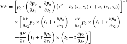 \begin{eqnarray}\boldsymbol{\nabla}F&=&\left[\boldsymbol{{p}}_0\boldsymbol{\cdot}\left(\frac{\partial\boldsymbol{{p}}_0}{\partial s_1}\times\frac{\partial\boldsymbol{{p}}_0}{\partial s_2}\right)\left(\tau^2+b_3\left(s_1,s_2\right)\tau+a_3\left(s_1,s_2\right)\right)\right]^{-1}\nonumber\\[3pt]&&\times\left[\frac{\partial F}{\partial s_2}\boldsymbol{{p}}_0\times\left(\boldsymbol{{t}}_1+\tau \frac{\partial\boldsymbol{{p}}_0}{\partial s_1}\right)-\frac{\partial F}{\partial s_1}\boldsymbol{{p}}_0\times\left(\boldsymbol{{t}}_2+\tau \frac{\partial\boldsymbol{{p}}_0}{\partial s_2}\right)\right.\nonumber\\[3pt]&&\left.+\frac{\partial F}{\partial \tau}\left(\boldsymbol{{t}}_1+\tau \frac{\partial\boldsymbol{{p}}_0}{\partial s_1}\right)\times\left(\boldsymbol{{t}}_2+\tau \frac{\partial\boldsymbol{{p}}_0}{\partial s_2}\right)\right]\end{eqnarray}
for any scalar function F and
 $a_3(\boldsymbol{{s}})$
and
$a_3(\boldsymbol{{s}})$
and
 $b_3(\boldsymbol{{s}})$
are known functions that are specific to this three-dimensional analysis (hence the subscription of ‘3’). These functions are
$b_3(\boldsymbol{{s}})$
are known functions that are specific to this three-dimensional analysis (hence the subscription of ‘3’). These functions are
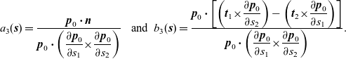 \begin{eqnarray}a_3(\boldsymbol{{s}})=\frac{\boldsymbol{{p}}_0\boldsymbol{\cdot}\boldsymbol{{n}}}{\displaystyle{\boldsymbol{{p}}_0\boldsymbol{\cdot}\left(\frac{\partial\boldsymbol{{p}}_0}{\partial s_1}{\times}\frac{\partial\boldsymbol{{p}}_0}{\partial s_2}\right)}}&\ \ \mbox{and}\ \ b_3(\boldsymbol{{s}})=\frac{\displaystyle{\boldsymbol{{p}}_0\boldsymbol{\cdot}\left[\left(\boldsymbol{{t}}_1{\times}\frac{\partial\boldsymbol{{p}}_0}{\partial s_2}\right)-\left(\boldsymbol{{t}}_2{\times}\frac{\partial\boldsymbol{{p}}_0}{\partial s_1}\right)\right]}}{\displaystyle{\boldsymbol{{p}}_0\boldsymbol{\cdot}\left(\frac{\partial\boldsymbol{{p}}_0}{\partial s_1}{\times}\frac{\partial\boldsymbol{{p}}_0}{\partial s_2}\right)}}.\end{eqnarray}
As noted above, the differential operator
 $\boldsymbol{\nabla}v_1\boldsymbol{\cdot}\boldsymbol{\nabla}$
is equivalent to
$\boldsymbol{\nabla}v_1\boldsymbol{\cdot}\boldsymbol{\nabla}$
is equivalent to
 $\displaystyle{\frac{d\;}{d\tau}}$
. Therefore, the leading-order transport equation (2.4) (with
$\displaystyle{\frac{d\;}{d\tau}}$
. Therefore, the leading-order transport equation (2.4) (with
 $n=0$
) reduces to a first-order ordinary differential equation along each ray
$n=0$
) reduces to a first-order ordinary differential equation along each ray
 \begin{eqnarray}\frac{d\boldsymbol{{E}}_0}{d\tau}+\frac{\left(2\tau+b_3(\boldsymbol{{s}})\right)\boldsymbol{{E}}_0}{2\!\left(\tau^2+b_3(\boldsymbol{{s}})\tau+a_3(\boldsymbol{{s}})\right)}&=&\textbf{0}.\end{eqnarray}
Equation (2.11) can easily be solved to give the general solution
 \begin{eqnarray}\boldsymbol{{E}}_0\left(\boldsymbol{{s}},\tau\right)&=&\boldsymbol{{e}}_0(\boldsymbol{{s}})\sqrt{\frac{a_3}{\tau^2+b_3\tau+a_3}},\end{eqnarray}
where
 $\boldsymbol{{e}}_0(\boldsymbol{{s}})$
is some given data for
$\boldsymbol{{e}}_0(\boldsymbol{{s}})$
is some given data for
 $\boldsymbol{{E}}_0$
at the point
$\boldsymbol{{E}}_0$
at the point
 $\tau=0$
. This process may be repeated to obtain an equivalent solution for
$\tau=0$
. This process may be repeated to obtain an equivalent solution for
 $\boldsymbol{{H}}_0$
. The leading-order solution is now determined; in principle, it is possible to obtain higher-order corrections in a recursive manner by using equations (2.4) and (2.5) .
$\boldsymbol{{H}}_0$
. The leading-order solution is now determined; in principle, it is possible to obtain higher-order corrections in a recursive manner by using equations (2.4) and (2.5) .
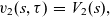
Modifications are required to ansätze (2.3) when, for instance, the rays associated with the incoming field contain additional terms in the exponent (for example, Tew’s work [Reference Tew17, Reference Tew18] on perturbed boundaries). It is possible to modify ansätze to include one additional term in the exponent proportional to
 $k^{\alpha}$
akin to the Friedlander–Keller ansatz (1.8). Doing so, however, quickly leads to the same conclusions that Friedlander & Keller [Reference Friedlander and Keller5] and Tew [Reference Tew17] came to – that power of
$k^{\alpha}$
akin to the Friedlander–Keller ansatz (1.8). Doing so, however, quickly leads to the same conclusions that Friedlander & Keller [Reference Friedlander and Keller5] and Tew [Reference Tew17] came to – that power of
 $\alpha$
must be
$\alpha$
must be
 $\displaystyle{\frac{1}{2}}$
in order to produce a leading-order change and the same arguments about the term appearing at
$\displaystyle{\frac{1}{2}}$
in order to produce a leading-order change and the same arguments about the term appearing at
 $O\!\left(k^{\alpha}\right)$
being constant if
$O\!\left(k^{\alpha}\right)$
being constant if
 $\displaystyle{\alpha>\frac{1}{2}}$
. It is clear from the work by Tew [Reference Tew18] that the Friedlander–Keller ansatz (1.8) must be generalised to accommodate a broader range of wave phenomena. Therefore, if N terms are present in the exponent (ranging from
$\displaystyle{\alpha>\frac{1}{2}}$
. It is clear from the work by Tew [Reference Tew18] that the Friedlander–Keller ansatz (1.8) must be generalised to accommodate a broader range of wave phenomena. Therefore, if N terms are present in the exponent (ranging from
 $O\!\left(k\right)$
,
$O\!\left(k\right)$
,
 $O\!\left(k^{\left(N-1\right)/N}\right)$
,
$O\!\left(k^{\left(N-1\right)/N}\right)$
,
 $\cdots O\!\left(k^{1/N}\right)$
), then Maxwell’s equations (2.1) and (2.2) will also contain terms starting at
$\cdots O\!\left(k^{1/N}\right)$
), then Maxwell’s equations (2.1) and (2.2) will also contain terms starting at
 $O\!\left(k\right)$
and decreasing in powers of
$O\!\left(k\right)$
and decreasing in powers of
 $k^{1/N}$
. This motivates the ansätze
$k^{1/N}$
. This motivates the ansätze
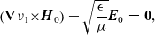
 \begin{eqnarray}\boldsymbol{{E}}&\sim&\exp\left(i\sum_{m=1}^N\;k^{\left(N+1-m\right)/N}v_m(\boldsymbol{{x}})\right)\sum_{n=0}^\infty\;\frac{\boldsymbol{{E}}_n(\boldsymbol{{x}})}{k^{n/N}}\mbox{, and }\nonumber\\\boldsymbol{{H}}&\sim&\exp\left(i\sum_{m=1}^N\;k^{\left(N+1-m\right)/N}v_m(\boldsymbol{{x}})\right)\sum_{n=0}^\infty\;\frac{\boldsymbol{{H}}_n(\boldsymbol{{x}})}{k^{n/N}}.\end{eqnarray}
Substitution of ansätze (2.13) into Maxwell’s equations (2.2) yields the following set of relations, which will be called upon regularly throughout the derivation. These relations are
 \begin{eqnarray}ik\left(\boldsymbol{\nabla}v_1\boldsymbol{\cdot}\boldsymbol{{E}}_0\right)+i\sum_{m=1}^{N-1}k^{\left(N-m\right)/N}\sum_{n=0}^m\left(\boldsymbol{\nabla}v_{m+1-n}\boldsymbol{\cdot}\boldsymbol{{E}}_n\right)&&\nonumber\\+\sum_{p=0}^\infty k^{-p/N}\left[\left(\boldsymbol{\nabla}\boldsymbol{\cdot}\boldsymbol{{E}}_p\right)+i\sum_{n=1}^N\left(\boldsymbol{\nabla}v_{N+1-n}\boldsymbol{\cdot}\boldsymbol{{E}}_{n+p}\right)\right]&=&0,\end{eqnarray}
which have been deliberately expressed in this way so that the first term appears is at
 $O\!\left(k\right)$
, the second term contains all terms between
$O\!\left(k\right)$
, the second term contains all terms between
 $O\!\left(k^{\left(N-1\right)/N}\right)$
and
$O\!\left(k^{\left(N-1\right)/N}\right)$
and
 $O\!\left(k^{1/N}\right)$
, and the final term contains all terms appearing at
$O\!\left(k^{1/N}\right)$
, and the final term contains all terms appearing at
 $O\!\left(1\right)$
and lower. A similar set of equations appear for the magnetic field.
$O\!\left(1\right)$
and lower. A similar set of equations appear for the magnetic field.
It is Maxwell’s equations (2.1) that will give the sought after field equations for the exponent terms and the transport equations. Applying the ansätze gives
 \begin{eqnarray}&&ik\left[\left(\boldsymbol{\nabla}v_1{\times}\boldsymbol{{E}}_0\right)-\sqrt{\frac{\mu}{\epsilon}}\boldsymbol{{H}}_0\right]+i\sum_{m=1}^{N-1}\;k^{\left(N-m\right)/N}\left[\sum_{n=0}^m\left(\boldsymbol{\nabla}v_{m+1-n}{\times}\boldsymbol{{E}}_n\right)-\sqrt{\frac{\mu}{\epsilon}}\boldsymbol{{H}}_m\right]\nonumber\\&&+\sum_{p=0}^\infty\;k^{-p/N}\left[\sum_{n=1}^N i\left(\boldsymbol{\nabla}v_{N+1-p}{\times}\boldsymbol{{E}}_{n+p}\right)+\left(\boldsymbol{\nabla}{\times}\boldsymbol{{E}}_p\right)-i\sqrt{\frac{\mu}{\epsilon}}\boldsymbol{{H}}_{N+p}\right]=\textbf{0},\end{eqnarray}
 \begin{eqnarray}&&ik\left[\left(\boldsymbol{\nabla}v_1{\times}\boldsymbol{{H}}_0\right)+\sqrt{\frac{\epsilon}{\mu}}\boldsymbol{{E}}_0\right]+i\sum_{m=1}^{N-1}\;k^{\left(N-m\right)/N}\left[\sum_{n=0}^m\left(\boldsymbol{\nabla}v_{m+1-n}{\times}\boldsymbol{{H}}_n\right)+\sqrt{\frac{\epsilon}{\mu}}\boldsymbol{{E}}_m\right]\nonumber\\&&+\sum_{p=0}^\infty\;k^{-p/N}\left[\sum_{n=1}^N i\left(\boldsymbol{\nabla}v_{N+1-p}{\times}\boldsymbol{{H}}_{n+p}\right)+\left(\boldsymbol{\nabla}{\times}\boldsymbol{{H}}_p\right)+i\sqrt{\frac{\epsilon}{\mu}}\boldsymbol{{E}}_{N+p}\right]=\textbf{0}.\end{eqnarray}
Again, these have been expressed so that the first term appears is at
 $O\!\left(k\right)$
, the second term contains all terms between
$O\!\left(k\right)$
, the second term contains all terms between
 $O\!\left(k^{\left(N-1\right)/N}\right)$
and
$O\!\left(k^{\left(N-1\right)/N}\right)$
and
 $O\!\left(k^{1/N}\right)$
, and the final term contains all terms appearing at
$O\!\left(k^{1/N}\right)$
, and the final term contains all terms appearing at
 $O\!\left(1\right)$
and lower. Comparing the terms at
$O\!\left(1\right)$
and lower. Comparing the terms at
 $O\!\left(k\right)$
in equations (2.15) and (2.16) gives that
$O\!\left(k\right)$
in equations (2.15) and (2.16) gives that
 \begin{eqnarray}\left(\boldsymbol{\nabla}v_1{\times}\boldsymbol{{H}}_0\right)+\sqrt{\frac{\epsilon}{\mu}}\boldsymbol{{E}}_0&=&\textbf{0},\end{eqnarray}
 \begin{eqnarray}\left(\boldsymbol{\nabla}v_1{\times}\boldsymbol{{E}}_0\right)-\sqrt{\frac{\mu}{\epsilon}}\boldsymbol{{H}}_0&=&\textbf{0}.\end{eqnarray}
Taking scalar products of
 $\boldsymbol{\nabla}v_1$
with either of equations (2.17) or (2.18) quickly gives that
$\boldsymbol{\nabla}v_1$
with either of equations (2.17) or (2.18) quickly gives that
 $\left[\boldsymbol{{E}}_0,\boldsymbol{{H}}_0,\boldsymbol{\nabla}v_1\right]$
for an orthogonal set. Moreover, eliminating
$\left[\boldsymbol{{E}}_0,\boldsymbol{{H}}_0,\boldsymbol{\nabla}v_1\right]$
for an orthogonal set. Moreover, eliminating
 $\boldsymbol{{H}}_0$
in these equations reveals that
$\boldsymbol{{H}}_0$
in these equations reveals that
 $v_1$
still satisfies the eikonal equation (1.3) . Therefore, solution (1.6) and the arguments surrounding it are still valid.
$v_1$
still satisfies the eikonal equation (1.3) . Therefore, solution (1.6) and the arguments surrounding it are still valid.
The following derivations are highly non-trivial and, as such, are provided in full detail in the Appendix to this paper. The main idea is to use equation (2.15) to express the various magnetic vectors as products of electric vectors and the gradient of the various exponent terms. Equation (2.16) then gives sets of equations involving only
 $\boldsymbol{\nabla}v$
and
$\boldsymbol{\nabla}v$
and
 $\boldsymbol{{E}}$
functions. It is the second set of terms in equations (2.15) and (2.16) (i.e. all terms appearing between
$\boldsymbol{{E}}$
functions. It is the second set of terms in equations (2.15) and (2.16) (i.e. all terms appearing between
 $O\!\left(k^{\left(N-1\right)/N}\right)$
and
$O\!\left(k^{\left(N-1\right)/N}\right)$
and
 $O\!\left(k^{1/N}\right)$
) that yield the field partial differential equations for the exponent terms; these are
$O\!\left(k^{1/N}\right)$
) that yield the field partial differential equations for the exponent terms; these are
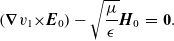
 \begin{eqnarray}\sum_{j=0}^n\!\left(\boldsymbol{\nabla}v_{n+1-j}\boldsymbol{\cdot}\boldsymbol{\nabla}v_{j+1}\right)&=&0,\mbox{ for }n=1,2,\cdots,N-1.\end{eqnarray}
Combining equations (1.3) and (2.19) yields a single recursive system of partial differential equations for all N exponent terms.
 \begin{eqnarray}\sum_{p=1}^n\!\left(\boldsymbol{\nabla}v_{n+1-p}\boldsymbol{\cdot}\boldsymbol{\nabla}v_p\right)&=&\delta_{1,n},\mbox{ for }n=1,2,\cdots N,\end{eqnarray}
with
 $\delta$
acting as the Kronecker delta.
$\delta$
acting as the Kronecker delta.
Following a similar methodology, it is the final group of terms in equations (2.15) and (2.16) that will provide the transport equations for the electric
 $\boldsymbol{{E}}$
vectors. The transport equation for a single electric vector
$\boldsymbol{{E}}$
vectors. The transport equation for a single electric vector
 $\boldsymbol{{E}}_q$
is
$\boldsymbol{{E}}_q$
is
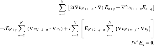 \begin{eqnarray}\sum_{n=1}^N\;\left[2\!\left(\boldsymbol{\nabla}v_{N+1-n}\boldsymbol{\cdot}\boldsymbol{\nabla}\right)\boldsymbol{{E}}_{n+q}+\nabla^2v_{N+1-n}\boldsymbol{{E}}_{n+q}\right]&&\nonumber\\&&\nonumber\\+i\boldsymbol{{E}}_{N+q}\sum_{n=2}^N\;\left(\boldsymbol{\nabla}v_{N+2-n}\boldsymbol{\cdot}\boldsymbol{\nabla}v_n\right)+i\sum_{n=3}^N\;\left[\boldsymbol{{E}}_{N+2+q-n}\sum_{j=n}^N\;\left(\boldsymbol{\nabla}v_{N+m-j}\boldsymbol{\cdot}\boldsymbol{\nabla}v_j\right)\right]&&\nonumber\\-i\nabla^2\boldsymbol{{E}}_q=\textbf{0}.&&\end{eqnarray}
This is a generic transport equation for
 $q\geq -N$
, as long as the vectors
$q\geq -N$
, as long as the vectors
 $\boldsymbol{{E}}_{-i}$
(
$\boldsymbol{{E}}_{-i}$
(
 $i=1,\cdots,N$
) are interpreted as null vectors. This is a recursive set of equations that is kick-started by the leading-order transport equation, which is
$i=1,\cdots,N$
) are interpreted as null vectors. This is a recursive set of equations that is kick-started by the leading-order transport equation, which is
 \begin{eqnarray}\frac{d\boldsymbol{{E}}_0}{d\tau}+\frac{1}{2}\left[\nabla^2v_1+i\sum_{n=2}^N\left(\boldsymbol{\nabla}v_{N+2-n}\boldsymbol{\cdot}\boldsymbol{\nabla}v_n\right)\right]\boldsymbol{{E}}_0&=&0,\end{eqnarray}
where the ray derivative relation
 $\displaystyle{\boldsymbol{\nabla}v_1\boldsymbol{\cdot}\boldsymbol{\nabla}=\frac{d\;}{d\tau}}$
has been used. This is a simple, first-order ordinary differential equation along a ray
$\displaystyle{\boldsymbol{\nabla}v_1\boldsymbol{\cdot}\boldsymbol{\nabla}=\frac{d\;}{d\tau}}$
has been used. This is a simple, first-order ordinary differential equation along a ray
 $\Gamma$
and has the integral solution
$\Gamma$
and has the integral solution
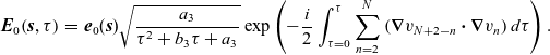 \begin{eqnarray}\boldsymbol{{E}}_0\!\left(\boldsymbol{{s}},\tau\right)&=&\boldsymbol{{e}}_0(\boldsymbol{{s}})\sqrt{\frac{a_3}{\tau^2+b_3\tau+a_3}}\exp\left(-\frac{i}{2}\int_{\tau=0}^\tau\sum_{n=2}^N\left(\boldsymbol{\nabla}v_{N+2-n}\boldsymbol{\cdot}\boldsymbol{\nabla}v_n\right)d\tau\right).\end{eqnarray}
It is possible to start from the beginning and repeat the procedure by eliminating the electric field to obtain a transport equation for each magnetic vector. Alternatively, as equations (2.15) and (2.16) are symmetric under the replacement of
 $\left[\boldsymbol{{E}},\boldsymbol{{H}},\epsilon,\mu\right]$
with
$\left[\boldsymbol{{E}},\boldsymbol{{H}},\epsilon,\mu\right]$
with
 $\left[\boldsymbol{{H}},\boldsymbol{{E}},-\mu,-\epsilon\right]$
, the magnetic transport equation to be written directly as
$\left[\boldsymbol{{H}},\boldsymbol{{E}},-\mu,-\epsilon\right]$
, the magnetic transport equation to be written directly as
 \begin{eqnarray}\sum_{n=1}^N\;\left[2\!\left(\boldsymbol{\nabla}v_{N+1-n}\boldsymbol{\cdot}\boldsymbol{\nabla}\right)\boldsymbol{{H}}_{n+q}+\nabla^2v_{N+1-n}\boldsymbol{{H}}_{n+q}\right]&&\nonumber\\&&\nonumber\\+i\boldsymbol{{H}}_{N+q}\sum_{n=2}^N\;\left(\boldsymbol{\nabla}v_{N+2-n}\boldsymbol{\cdot}\boldsymbol{\nabla}v_n\right)+i\sum_{n=3}^N\;\left[\boldsymbol{{H}}_{N+2+q-n}\sum_{j=n}^N\;\left(\boldsymbol{\nabla}v_{N+m-j}\boldsymbol{\cdot}\boldsymbol{\nabla}v_j\right)\right]&&\nonumber\\-i\nabla^2\boldsymbol{{H}}_q=\textbf{0}.&&\end{eqnarray}
Similarly,
 $\boldsymbol{{H}}_0$
has an identical leading-order transport equation and solution to that for the leading-order electric vector
$\boldsymbol{{H}}_0$
has an identical leading-order transport equation and solution to that for the leading-order electric vector
 $\boldsymbol{{E}}_0$
:
$\boldsymbol{{E}}_0$
:
 \begin{eqnarray}\boldsymbol{{H}}_0\!\left(\boldsymbol{{s}},\tau\right)&=&\boldsymbol{{h}}_0(\boldsymbol{{s}})\sqrt{\frac{a_3}{\tau^2+b_3\tau+a_3}}\exp\left(-\frac{i}{2}\int_{\tau=0}^\tau\sum_{n=2}^N\left(\boldsymbol{\nabla}v_{N+2-n}\boldsymbol{\cdot}\boldsymbol{\nabla}v_n\right)d\tau\right).\end{eqnarray}
Here,
 $\boldsymbol{{h}}_0$
is some given/calculable boundary data on
$\boldsymbol{{h}}_0$
is some given/calculable boundary data on
 $\tau=0$
and is related to
$\tau=0$
and is related to
 $\boldsymbol{{e}}_0$
by equation (2.18), and the integral is solved by using identity (2.9). Note that the ‘square-root’ pre-factor is identical to the classical case appearing in solution (2.12). In the context of waves, this shows that the presence of additional exponent terms in the original ansätze does not change the leading-order amplitude, but it is now accompanied by an
$\boldsymbol{{e}}_0$
by equation (2.18), and the integral is solved by using identity (2.9). Note that the ‘square-root’ pre-factor is identical to the classical case appearing in solution (2.12). In the context of waves, this shows that the presence of additional exponent terms in the original ansätze does not change the leading-order amplitude, but it is now accompanied by an
 $O\!\left(1\right)$
phase correction. Naturally, fixing
$O\!\left(1\right)$
phase correction. Naturally, fixing
 $v_2,\cdots,v_N\equiv 0$
reduces solution (2.23) to the classic solution (2.12), and similarly for
$v_2,\cdots,v_N\equiv 0$
reduces solution (2.23) to the classic solution (2.12), and similarly for
 $\boldsymbol{{H}}_0$
.
$\boldsymbol{{H}}_0$
.
Although it is possible to continue developing the ‘general N’ method and find generic applications for this theory, it is more illustrative to specify the value of N in a variety of problems and then demonstrate the method surrounding these problems. Two distinct situations are of natural importance. The first is to have the geometry of the wave-front prescribed with ‘natural’ wave-fronts (planar or spherical, for instance), which is mathematically similar to prescribing the value of
 $v_1$
. The other situation is when data are imposed on a generic surface that may or may not conform to a wave-front. The theory presented above will now be used to address both of these sets of problems.
$v_1$
. The other situation is when data are imposed on a generic surface that may or may not conform to a wave-front. The theory presented above will now be used to address both of these sets of problems.
3 Solutions to prescribed wave-front problems
Fixing the value of
 $v_1(\boldsymbol{{x}})$
is equivalent to having the geometry of the wave-front prescribed, so this will now be done for
$v_1(\boldsymbol{{x}})$
is equivalent to having the geometry of the wave-front prescribed, so this will now be done for
 $\left(i\right)$
spherical wave-fronts,
$\left(i\right)$
spherical wave-fronts,
 $\left(ii\right)$
planar wave-fronts, and
$\left(ii\right)$
planar wave-fronts, and
 $\left(iii\right)$
arbitrary wave-fronts, each for a different arbitrarily chosen value of N to illustrate the diversity of the above theory.
$\left(iii\right)$
arbitrary wave-fronts, each for a different arbitrarily chosen value of N to illustrate the diversity of the above theory.
3.1 Spherical wave-fronts
Starting with an
 $N=2$
problem, equations (2.20) and (2.21) give three equations:
$N=2$
problem, equations (2.20) and (2.21) give three equations:
 \begin{eqnarray}\boldsymbol{\nabla}v_1\boldsymbol{\cdot}\boldsymbol{\nabla}v_1&=&1,\end{eqnarray}
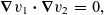
 \begin{eqnarray}\boldsymbol{\nabla}v_1\boldsymbol{\cdot}\boldsymbol{\nabla}v_2&=&0,\end{eqnarray}
 \begin{eqnarray}2\!\left(\boldsymbol{\nabla}v_1\boldsymbol{\cdot}\boldsymbol{\nabla}\right)\boldsymbol{{E}}_0+\boldsymbol{{E}}_0\left[\nabla^2v_1+i\left(\boldsymbol{\nabla}v_2\boldsymbol{\cdot}\boldsymbol{\nabla}v_2\right)\right]&=&0.\end{eqnarray}
Working with radially symmetric wave-fronts, which have an initial wave-front on
 $r=a$
, the leading-order exponent term is set to
$r=a$
, the leading-order exponent term is set to
 \begin{eqnarray}v_1\!\left(r,\theta,\psi\right)&=&r,\end{eqnarray}
which satisfies the eikonal equation (3.1) . The aim now is to construct expressions for
 $v_2$
and
$v_2$
and
 $\boldsymbol{{E}}_0$
in conjunction with this fixed value of
$\boldsymbol{{E}}_0$
in conjunction with this fixed value of
 $v_1$
. Continuing with spherical-polar coordinates, equation (3.2) becomes
$v_1$
. Continuing with spherical-polar coordinates, equation (3.2) becomes
 \begin{eqnarray}\frac{\partial v_2}{\partial r}&=&0,\end{eqnarray}
which easily shows that
 $v_2$
depends only on
$v_2$
depends only on
 $\theta$
and
$\theta$
and
 $\psi$
and so has the general form
$\psi$
and so has the general form
 \begin{eqnarray}v_2\!\left(r,\theta,\psi\right)&=&V_2\!\left(\theta,\psi\right),\end{eqnarray}
for some arbitrary function
 $V_2$
. Equation (3.3) now yields the leading-order amplitude equation for
$V_2$
. Equation (3.3) now yields the leading-order amplitude equation for
 $\boldsymbol{{E}}_0$
:
$\boldsymbol{{E}}_0$
:
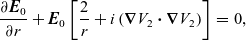 \begin{eqnarray}\frac{\partial\boldsymbol{{E}}_0}{\partial r}+\boldsymbol{{E}}_0\left[\frac{2}{r}+i\left(\boldsymbol{\nabla}V_2\boldsymbol{\cdot}\boldsymbol{\nabla}V_2\right)\right]&=&0,\end{eqnarray}
which is easily solved by introducing an integrating factor, and the solution is
 \begin{eqnarray}\boldsymbol{{E}}_0\!\left(r,\theta,\psi\right)&=&\frac{a}{r}\boldsymbol{{e}}_0\left(\theta,\psi\right)\exp\left(\frac{ir\left(a-r\right)}{2a}\left(\boldsymbol{\nabla}V_2\boldsymbol{\cdot}\boldsymbol{\nabla}V_2\right)\right).\end{eqnarray}
This completely solves, to leading order, the
 $N=2$
problem for spherical wave-front initially valid on
$N=2$
problem for spherical wave-front initially valid on
 $r=a$
. The
$r=a$
. The
 $\boldsymbol{{e}}_0$
appearing in solution (3.8) is the same as that which would appear in the application of standard ray theory (in which
$\boldsymbol{{e}}_0$
appearing in solution (3.8) is the same as that which would appear in the application of standard ray theory (in which
 $v_2\equiv 0$
).
$v_2\equiv 0$
).
3.2 Planar wave-fronts
Focusing now on an
 $N=3$
problem and fixing this value in equations (2.20) and (2.21) gives four field equations to consider, which are
$N=3$
problem and fixing this value in equations (2.20) and (2.21) gives four field equations to consider, which are
 \begin{eqnarray}\boldsymbol{\nabla}v_1\boldsymbol{\cdot}\boldsymbol{\nabla}v_1&=&1,\end{eqnarray}
 \begin{eqnarray}\boldsymbol{\nabla}v_1\boldsymbol{\cdot}\boldsymbol{\nabla}v_2&=&0,\end{eqnarray}
 \begin{eqnarray}2\!\left(\boldsymbol{\nabla}v_1\boldsymbol{\cdot}\boldsymbol{\nabla}v_3\right)+\left(\boldsymbol{\nabla}v_2\boldsymbol{\cdot}\boldsymbol{\nabla}v_2\right)&=&0,\end{eqnarray}
 \begin{eqnarray}2\!\left(\boldsymbol{\nabla}v_1\boldsymbol{\nabla}\right)\boldsymbol{{E}}_0+\boldsymbol{{E}}_0\left[\nabla^2v_1+2i\left(\boldsymbol{\nabla}v_2\boldsymbol{\cdot}\boldsymbol{\nabla}v_3\right)\right]&=&\textbf{0}.\end{eqnarray}
Working with planar wave-fronts, which are initially on the surface
 $z=0$
, the leading-order phase term is fixed to
$z=0$
, the leading-order phase term is fixed to
 \begin{eqnarray}v_1\!\left(x,y,z\right)&=&z,\end{eqnarray}
which satisfies eikonal equation (3.9) automatically. Similarly to before, the aim is to construct expressions for the additional exponent terms
 $v_2$
,
$v_2$
,
 $v_3$
, and
$v_3$
, and
 $\boldsymbol{{E}}_0$
in conjunction with this prescribed value of
$\boldsymbol{{E}}_0$
in conjunction with this prescribed value of
 $v_1$
. Equation (3.10) now becomes
$v_1$
. Equation (3.10) now becomes
 \begin{eqnarray}\frac{\partial v_2}{\partial z}&=&0;\end{eqnarray}
it is easily observed that
 $v_2$
is independent of z and so has the solution
$v_2$
is independent of z and so has the solution
 \begin{eqnarray}v_2\!\left(x,y,z\right)&=&V_2\!\left(x,y\right),\end{eqnarray}
for an arbitrary function
 $V_2$
. Equation (3.11) then simplifies to
$V_2$
. Equation (3.11) then simplifies to
 \begin{eqnarray}2\frac{\partial v_3}{\partial z}+\left(\boldsymbol{\nabla}V_2\boldsymbol{\cdot}\boldsymbol{\nabla}V_2\right)&=&0,\end{eqnarray}
which is easily solved by direct integration as
 $V_2$
is independent of z. Thus,
$V_2$
is independent of z. Thus,
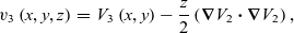 \begin{eqnarray}v_3\left(x,y,z\right)&=&V_3\left(x,y\right)-\frac{z}{2}\left(\boldsymbol{\nabla}V_2\boldsymbol{\cdot}\boldsymbol{\nabla}V_2\right),\end{eqnarray}
for some arbitrary function
 $V_3$
. Turning now to the leading-order transport equation (3.12), which simplifies as
$V_3$
. Turning now to the leading-order transport equation (3.12), which simplifies as
 $\nabla^2v_1=0$
,
$\nabla^2v_1=0$
,
 $\boldsymbol{{E}}_0$
satisfies the field partial differential equation
$\boldsymbol{{E}}_0$
satisfies the field partial differential equation
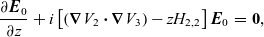 \begin{eqnarray}\frac{\partial\boldsymbol{{E}}_0}{\partial z}+i\left[\left(\boldsymbol{\nabla}V_2\boldsymbol{\cdot}\boldsymbol{\nabla}V_3\right)-zH_{2,2}\right]\boldsymbol{{E}}_0&=&\textbf{0},\end{eqnarray}
where
 $H_{2,2}$
is given as
$H_{2,2}$
is given as
 \begin{eqnarray}H_{2,2}&=&\left(\frac{\partial V_2}{\partial x}\right)^2\frac{\partial^2 V_2}{\partial x^2}+2\frac{\partial V_2}{\partial x}\frac{\partial V_2}{\partial y}\frac{\partial^2 V_2}{\partial x\partial y}+\left(\frac{\partial V_2}{\partial y}\right)^2\frac{\partial^2 V_2}{\partial y^2}.\end{eqnarray}
Equation (3.18) is easily solved with an integrating factor; the solution is
 \begin{eqnarray}\boldsymbol{{E}}_0\left(x,y,z\right)&=&\boldsymbol{{e}}_0\left(x,y\right)\exp\left(iz\left[\frac{z}{2}H_{2,2}-\left(\boldsymbol{\nabla}V_2\boldsymbol{\cdot}\boldsymbol{\nabla}V_3\right)\right]\right).\end{eqnarray}
This solution of the
 $N=3$
for planar wave-fronts is now fully constructed, and the
$N=3$
for planar wave-fronts is now fully constructed, and the
 $\boldsymbol{{e}}_0$
appearing in the solution (3.20) is the same that would appear in the application of classic ray theory in which
$\boldsymbol{{e}}_0$
appearing in the solution (3.20) is the same that would appear in the application of classic ray theory in which
 $v_2\equiv 0$
and
$v_2\equiv 0$
and
 $v_3\equiv 0$
.
$v_3\equiv 0$
.
3.3 Arbitrary wave-fronts
Unlike those wave-fronts considered before, which were simple geometries (a regular sphere and a flat plane), this particular investigation focuses on any initial surface that conforms to a wave-front. This particular surface is described parametrically as that considered in Section 2, so the geometric equations (2.7) hold. The content there specified rays
 $\Gamma$
, along which solutions were constructed. However, as rays are everywhere normal to wave-fronts, many simplifications can be made. Firstly, the ray direction
$\Gamma$
, along which solutions were constructed. However, as rays are everywhere normal to wave-fronts, many simplifications can be made. Firstly, the ray direction
 $\boldsymbol{{p}}_0$
is now normal. Hence, solution (2.8) now reduces to
$\boldsymbol{{p}}_0$
is now normal. Hence, solution (2.8) now reduces to
 \begin{eqnarray}\boldsymbol{{p}}_0&=&\boldsymbol{{n}}.\end{eqnarray}
This is an extremely useful result as the derivatives of
 $\boldsymbol{{p}}_0$
appearing in, for example, identity (2.9), will become derivatives of the normal vector. Defining the parameters
$\boldsymbol{{p}}_0$
appearing in, for example, identity (2.9), will become derivatives of the normal vector. Defining the parameters
 $s_1$
and
$s_1$
and
 $s_2$
as arc-length along their respective curves (leading to the arguments surrounding equations (2.7) ) will now allow a set of Frenet–Serret formulae to be used, which relate the normal vector
$s_2$
as arc-length along their respective curves (leading to the arguments surrounding equations (2.7) ) will now allow a set of Frenet–Serret formulae to be used, which relate the normal vector
 $\boldsymbol{{n}}$
to the two independent tangential vectors
$\boldsymbol{{n}}$
to the two independent tangential vectors
 $\boldsymbol{{t}}_i$
(for
$\boldsymbol{{t}}_i$
(for
 $i=1,2$
) by
$i=1,2$
) by
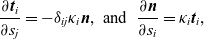 \begin{eqnarray}\frac{\partial\boldsymbol{{t}}_i}{\partial s_j}=-\delta_{ij}\kappa_i\boldsymbol{{n}},&\mbox{ and }&\frac{\partial\boldsymbol{{n}}}{\partial s_i}=\kappa_i\boldsymbol{{t}}_i,\end{eqnarray}
for
 $j=1,2$
and in which
$j=1,2$
and in which
 $\kappa_i$
denotes the curvature of a curve in the
$\kappa_i$
denotes the curvature of a curve in the
 $i{\rm th}$
principle direction. With this frame now fully established, identity (2.9) now reduces to
$i{\rm th}$
principle direction. With this frame now fully established, identity (2.9) now reduces to
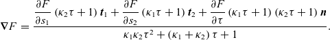 \begin{eqnarray}\boldsymbol{\nabla}F&=&\frac{\displaystyle{\frac{\partial F}{\partial s_1}\left(\kappa_2\tau+1\right)\boldsymbol{{t}}_1+\frac{\partial F}{\partial s_2}\left(\kappa_1\tau+1\right)\boldsymbol{{t}}_2+\frac{\partial F}{\partial \tau}\left(\kappa_1\tau+1\right)\left(\kappa_2\tau+1\right)\boldsymbol{{n}}}}{\kappa_1\kappa_2\tau^2+\left(\kappa_1+\kappa_2\right)\tau+1}.\end{eqnarray}
The scalar products of the gradients of the various exponent terms appearing in equation (2.20), for example, are now given simply as
 \begin{eqnarray}\boldsymbol{\nabla}v_p\boldsymbol{\cdot}\boldsymbol{\nabla}v_j&=&\left[\kappa_1\kappa_2\tau^2+\left(\kappa_1+\kappa_2\right)\tau+1\right]^{-2}\left(\frac{\partial v_p}{\partial \tau}\frac{\partial v_j}{\partial \tau}\left(\kappa_1\tau+1\right)^2\!\left(\kappa_2\tau+1\right)^2\right.\nonumber\\&&\left.+\frac{\partial v_p}{\partial s_1}\frac{\partial v_j}{\partial s_1}\left(\kappa_2\tau+1\right)^2+\frac{\partial v_p}{\partial s_2}\frac{\partial v_j}{\partial s_2}\left(\kappa_1\tau+1\right)^2\right).\end{eqnarray}
As the leading-order phase term,
 $v_1$
still satisfies the eikonal equation (1.3), then
$v_1$
still satisfies the eikonal equation (1.3), then
 $v_1$
is still satisfied by solution (1.6); the argument surrounding it also applies. Therefore, the differential operator
$v_1$
is still satisfied by solution (1.6); the argument surrounding it also applies. Therefore, the differential operator
 $\left(\boldsymbol{\nabla}v_1\boldsymbol{\cdot}\boldsymbol{\nabla}\right)$
is the ordinary derivative along any ray
$\left(\boldsymbol{\nabla}v_1\boldsymbol{\cdot}\boldsymbol{\nabla}\right)$
is the ordinary derivative along any ray
 $\Gamma\left(\tau\right)$
. Hence, the solution to the remaining exponent terms is expressed as the integral equation
$\Gamma\left(\tau\right)$
. Hence, the solution to the remaining exponent terms is expressed as the integral equation
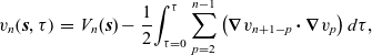 \begin{eqnarray}v_n\!\left(\boldsymbol{{s}},\tau\right)&=&V_n(\boldsymbol{{s}})-\frac{1}{2}\displaystyle{\int_{\tau=0}^\tau\sum_{p=2}^{n-1}\left(\boldsymbol{\nabla}v_{n+1-p}\boldsymbol{\cdot}\boldsymbol{\nabla}v_p\right)d\tau},\end{eqnarray}
for
 $n=2,\cdots,N$
and where
$n=2,\cdots,N$
and where
 $V_n(\boldsymbol{{s}})$
is the value of
$V_n(\boldsymbol{{s}})$
is the value of
 $v_n$
at the point
$v_n$
at the point
 $\tau=0$
, which is on the initial wave-front
$\tau=0$
, which is on the initial wave-front
 $\boldsymbol{{x}}_0$
.
$\boldsymbol{{x}}_0$
.
As a direct result of this Frenet–Serret frame, the known surface functions
 $a_3$
and
$a_3$
and
 $b_3$
in equation (2.10) reduce to the simple expressions
$b_3$
in equation (2.10) reduce to the simple expressions
 \begin{eqnarray}a_3=\frac{1}{\kappa_1 \kappa_2},&\mbox{ and }&b_3=\frac{\kappa_1+\kappa_2}{\kappa_1 \kappa_2},\end{eqnarray}
so that
 $a_3$
is the inverse of the Gaussian curvature of
$a_3$
is the inverse of the Gaussian curvature of
 $\boldsymbol{{x}}_0$
and
$\boldsymbol{{x}}_0$
and
 $b_3$
is twice the ratio of the mean and Gaussian curvatures of
$b_3$
is twice the ratio of the mean and Gaussian curvatures of
 $\boldsymbol{{x}}_0$
. Hence, the leading-order solution (2.23) now becomes
$\boldsymbol{{x}}_0$
. Hence, the leading-order solution (2.23) now becomes
 \begin{eqnarray}\boldsymbol{{E}}_0\left(\boldsymbol{{s}},\tau\right)&=&\frac{\boldsymbol{{e}}_0(\boldsymbol{{s}})}{\sqrt{\left(\kappa_1\tau+1\right)\left(\kappa_2\tau+1\right)}}\exp\left(-\frac{i}{2}\int_{\tau=0}^\tau\sum_{n=2}^N\left(\boldsymbol{\nabla}v_{N+2-n}\boldsymbol{\cdot}\boldsymbol{\nabla}v_n\right)\right).\end{eqnarray}
Fixing
 $v_i\equiv 0$
 $\left(i=2,3,\cdots,N\right)$
, to conform with the classical theory and using the fact that curvature is related to the radius of curvature by
$\left(i=2,3,\cdots,N\right)$
, to conform with the classical theory and using the fact that curvature is related to the radius of curvature by
 $\kappa_i=\rho_i^{-1}$
, solution (3.27) reduces to the vectorial form of Levy & Keller’s solution (1.7) [Reference Levy and Keller11] and also conforms to the wave-front solutions obtained by Molinet et al. [Reference Molinet, Andronov and Bouche13].
$\kappa_i=\rho_i^{-1}$
, solution (3.27) reduces to the vectorial form of Levy & Keller’s solution (1.7) [Reference Levy and Keller11] and also conforms to the wave-front solutions obtained by Molinet et al. [Reference Molinet, Andronov and Bouche13].
This solution method will be illustrated by picking a specific value of
 $N=3$
. In this case, the equations to solve are identical to those appearing in equations (3.9)–(3.12) . As this is now a generic wave-front, there is no specified form of
$N=3$
. In this case, the equations to solve are identical to those appearing in equations (3.9)–(3.12) . As this is now a generic wave-front, there is no specified form of
 $v_1$
, so the general solution for this term is given by solution (1.6). Owing to the differential operator
$v_1$
, so the general solution for this term is given by solution (1.6). Owing to the differential operator
 $\left(\boldsymbol{\nabla}v_1\boldsymbol{\cdot}\boldsymbol{\nabla}\right)$
being the ordinary derivative along any ray, equation (3.10) gives that
$\left(\boldsymbol{\nabla}v_1\boldsymbol{\cdot}\boldsymbol{\nabla}\right)$
being the ordinary derivative along any ray, equation (3.10) gives that
 $v_2$
is constant along each ray and depends solely on the point from which that ray emanates. Thus,
$v_2$
is constant along each ray and depends solely on the point from which that ray emanates. Thus,
 \begin{eqnarray}v_2\!\left(\boldsymbol{{s}},\tau\right)&=&V_2(\boldsymbol{{s}}).\end{eqnarray}
Given this solution, equation (3.11) becomes
 \begin{eqnarray}2\frac{d v_3}{d\tau}+\left(\frac{1}{1+\kappa_1\tau}\right)^2\!\left(\frac{\partial V_2}{\partial s_1}\right)^2+\left(\frac{1}{1+\kappa_2\tau}\right)^2\!\left(\frac{\partial V_2}{\partial s_2}\right)^2&=&0.\end{eqnarray}
This can be solved by directly integrating along the rays to give the solution
 \begin{eqnarray}v_3\!\left(\boldsymbol{{s}},\tau\right)&=&V_3(\boldsymbol{{s}})-\frac{\tau}{2}\left[\frac{1}{1+\kappa_1\tau}\left(\frac{\partial V_2}{\partial s_1}\right)^2+\frac{1}{1+\kappa_2\tau}\left(\frac{\partial V_2}{\partial s_2}\right)^2\right].\end{eqnarray}
With these solutions known, attention now is on the transport equation (3.12) for
 $\boldsymbol{{E}}_0$
; this becomes
$\boldsymbol{{E}}_0$
; this becomes
 \begin{eqnarray}2\frac{d\boldsymbol{{E}}_0}{d\tau}+\boldsymbol{{E}}_0\left[\frac{2\tau+b_3}{\tau^2+b_3\tau+a_3}+2i\sum_{i=1}^2\left[\frac{\partial V_2}{\partial s_i}\frac{\partial V_3}{\partial s_i}\left(1+\kappa_i\tau\right)^{-2}\right.\right.&&\nonumber\\\left.\left.-\tau\left(\left(\frac{\partial V_2}{\partial s_i}\right)^2\frac{\partial^2 V_2}{\partial s_i^2}\left(1+\kappa_i\tau\right)^{-3}\right.\right.\right.&&\nonumber\\\left.\left.\left.+\frac{\partial V_2}{\partial s_i}\frac{\partial V_2}{\partial s_{3-i}}\frac{\partial^2 V_2}{\partial s_i\partial s_{3-i}}\left(1+\kappa_i\tau\right)^2\!\left(1+\kappa_{3-i}\tau\right)\right)\right]\right]&=&\textbf{0}.\end{eqnarray}
This can be solved by introducing an integrating factor, and the solution can be expressed in the compact form
 \begin{eqnarray}\boldsymbol{{E}}_0\!\left(\boldsymbol{{s}},\tau\right)&=&\frac{\boldsymbol{{e}}_0(\boldsymbol{{s}})}{\sqrt{\left(\kappa_1\tau+1\right)\left(\kappa_2\tau+1\right)}}\exp\!\left(\frac{i\tau}{2}\left[\tau H_{2,2}-2H_{1,3}\right]\right),\end{eqnarray}
in which
 \begin{eqnarray}H_{1,3}&=&\frac{1}{\kappa_1\tau+1}\frac{\partial V_2}{\partial s_1}\frac{\partial V_3}{\partial s_1}+\frac{1}{\kappa_2\tau+1}\frac{\partial V_2}{\partial s_2}\frac{\partial V_3}{\partial s_2},\end{eqnarray}
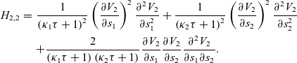 \begin{eqnarray}H_{2,2}&=&\frac{1}{\left(\kappa_1\tau+1\right)^2}\left(\frac{\partial V_2}{\partial s_1}\right)^2\frac{\partial^2 V_2}{\partial s_1^2}+\frac{1}{\left(\kappa_2\tau+1\right)^2}\left(\frac{\partial V_2}{\partial s_2}\right)^2\frac{\partial^2 V_2}{\partial s_2^2}\nonumber\\&&+\frac{2}{\left(\kappa_1\tau+1\right)\left(\kappa_2\tau+1\right)}\frac{\partial V_2}{\partial s_1}\frac{\partial V_2}{\partial s_2}\frac{\partial^2 V_2}{\partial s_1 \partial s_2}.\end{eqnarray}
This completes the example of the arbitrary wave-front
 $N=3$
problem to leading order.
$N=3$
problem to leading order.
One specific example here is to assign the wave-front the parametrisation
 $\boldsymbol{{x}}_0=\left[s_1,s_2,0\right]$
, that is, a flat plane, so that the two curvatures
$\boldsymbol{{x}}_0=\left[s_1,s_2,0\right]$
, that is, a flat plane, so that the two curvatures
 $\kappa_1$
and
$\kappa_1$
and
 $\kappa_2$
are both equal to zero. The associated waves are, therefore, planar. In this case,
$\kappa_2$
are both equal to zero. The associated waves are, therefore, planar. In this case,
 $V_1$
is simply 0, so that
$V_1$
is simply 0, so that
 $v_1=\tau$
. Moreover, the gradient operator (3.23) becomes
$v_1=\tau$
. Moreover, the gradient operator (3.23) becomes
 \begin{eqnarray}\boldsymbol{\nabla}F&=&\left[\frac{\partial F}{\partial s_1},\frac{\partial F}{\partial s_2},\frac{\partial F}{\partial \tau}\right].\end{eqnarray}
The second exponent term
 $v_2$
is given by solution (3.28), and the final exponent term
$v_2$
is given by solution (3.28), and the final exponent term
 $v_3$
now reduces to
$v_3$
now reduces to
 \begin{eqnarray}v_3\left(\boldsymbol{{s}},\tau\right)&=&V_3(\boldsymbol{{s}})-\frac{\tau}{2}\left[\left(\frac{\partial V_2}{\partial s_1}\right)^2+\left(\frac{\partial V_2}{\partial s_2}\right)^2\right].\end{eqnarray}
Finally, the leading-order amplitude becomes
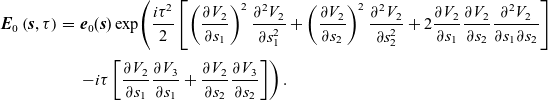 \begin{eqnarray}\boldsymbol{{E}}_0\left(\boldsymbol{{s}},\tau\right)&=&\boldsymbol{{e}}_0(\boldsymbol{{s}})\exp\!\left(\frac{i\tau^2}{2}\left[\left(\frac{\partial V_2}{\partial s_1}\right)^2\frac{\partial^2 V_2}{\partial s_1^2}+\left(\frac{\partial V_2}{\partial s_2}\right)^2\frac{\partial^2 V_2}{\partial s_2^2}+2\frac{\partial V_2}{\partial s_1}\frac{\partial V_2}{\partial s_2}\frac{\partial^2 V_2}{\partial s_1\partial s_2}\right]\right.\nonumber\\[3pt]&&\left.-i\tau\left[\frac{\partial V_2}{\partial s_1}\frac{\partial V_3}{\partial s_1}+\frac{\partial V_2}{\partial s_2}\frac{\partial V_3}{\partial s_2}\right]\right).\end{eqnarray}
As a result of this parametrisation and operator (3.35), ray equations (2.6) now become
 $\boldsymbol{{x}}=\left[s_1,s_2,0\right]+\tau\left[0,0,1\right]$
, which allow the obtained results to be transformed back into Cartesian variables. Doing so returns the results obtained in subsection (3.2), as expected.
$\boldsymbol{{x}}=\left[s_1,s_2,0\right]+\tau\left[0,0,1\right]$
, which allow the obtained results to be transformed back into Cartesian variables. Doing so returns the results obtained in subsection (3.2), as expected.
4 Summary, conclusions, and discussion
This paper has focused on generalised Friedlander–Keller ray expansions in which the exponent terms of the ray ansatz contain all terms proportional to
 $k^{1/N}$
between
$k^{1/N}$
between
 $k^{1/N}$
and k, for a positive integer N. This follows on from the work of Tew [Reference Tew18], who considered an equivalent ray ansatz for scalar waves. Tew’s work is a generalisation of the original Friedlander–Keller ray expansion, which contained only one additional term in the exponent (a term in addition to that appearing at
$k^{1/N}$
and k, for a positive integer N. This follows on from the work of Tew [Reference Tew18], who considered an equivalent ray ansatz for scalar waves. Tew’s work is a generalisation of the original Friedlander–Keller ray expansion, which contained only one additional term in the exponent (a term in addition to that appearing at
 $O\!\left(k\right)$
) proportional to
$O\!\left(k\right)$
) proportional to
 $k^{\alpha}$
. Although their analysis showed that a non-constant additional exponent term requires
$k^{\alpha}$
. Although their analysis showed that a non-constant additional exponent term requires
 $\alpha$
to have a specific value in the range
$\alpha$
to have a specific value in the range
 $\displaystyle{0<\alpha\le \frac{1}{2}}$
, there were no restrictions on what value
$\displaystyle{0<\alpha\le \frac{1}{2}}$
, there were no restrictions on what value
 $\alpha$
could be in that range (rational or otherwise). Both the work here and that of Tew specified
$\alpha$
could be in that range (rational or otherwise). Both the work here and that of Tew specified
 $\alpha$
to be a rational number of the form
$\alpha$
to be a rational number of the form
 $\displaystyle{\alpha=\frac{n}{N}}$
, for a particular integer n in the range
$\displaystyle{\alpha=\frac{n}{N}}$
, for a particular integer n in the range
 $1\le n\le N-1$
.
$1\le n\le N-1$
.
Although the examples presented here specify the values
 $N=2$
and 3, the theory and methods apply to any value of N. However, it seems there is no generic solution for the exponent terms for an arbitrary value of N, beyond those given by integral solutions (3.25), and each value of N requires individual consideration. Nevertheless, when comparing the cases of
$N=2$
and 3, the theory and methods apply to any value of N. However, it seems there is no generic solution for the exponent terms for an arbitrary value of N, beyond those given by integral solutions (3.25), and each value of N requires individual consideration. Nevertheless, when comparing the cases of
 $N=N_0$
and
$N=N_0$
and
 $N=N_0+m$
(for arbitrary positive integers
$N=N_0+m$
(for arbitrary positive integers
 $N_0$
and m), equation (2.20) and solution (3.25) demonstrate that the first
$N_0$
and m), equation (2.20) and solution (3.25) demonstrate that the first
 $N_0$
exponent terms would be identical in both cases.
$N_0$
exponent terms would be identical in both cases.
One application of the findings in this paper is the scattering of an electric field which is incident upon a conducting surface. One of the many scattering examples which have been considered in the literature (Keller [Reference Keller, Lewis and Seckler10], for example) is a point source located at the focal point of a paraboloid. Suppose the point source is disturbed by
 $k^{-1/N}$
displacement, then the incident field will necessarily be of the generalised Friedlander–Keller form, which necessitates the scattered field also be of that form. If the surface is not a perfect conductor and is penetrable, then an extension to the theory contained in this paper is to boundaries that do not prevent the incident field from transmitting through, that is, a boundary which separates two distinct wave-bearing media which would give rise to refracted rays which would also be amenable to the theory presented here. This was briefly considered by Radjen et al. [Reference Radjen, Gradoni and Tew15], where the incident electric field encountered a ‘perturbed’ boundary (in the style of the language used there) which was penetrable and so resulted in a newly formed electric field outside of that boundary. This problem would involve two wave-numbers (one for each media); both total fields would each satisfy their own Maxwell’s equations (2.1) and (2.2) . The difference in wave-number would result in fundamental changes to, for example, the key eikonal equation, which would now have the solution
$k^{-1/N}$
displacement, then the incident field will necessarily be of the generalised Friedlander–Keller form, which necessitates the scattered field also be of that form. If the surface is not a perfect conductor and is penetrable, then an extension to the theory contained in this paper is to boundaries that do not prevent the incident field from transmitting through, that is, a boundary which separates two distinct wave-bearing media which would give rise to refracted rays which would also be amenable to the theory presented here. This was briefly considered by Radjen et al. [Reference Radjen, Gradoni and Tew15], where the incident electric field encountered a ‘perturbed’ boundary (in the style of the language used there) which was penetrable and so resulted in a newly formed electric field outside of that boundary. This problem would involve two wave-numbers (one for each media); both total fields would each satisfy their own Maxwell’s equations (2.1) and (2.2) . The difference in wave-number would result in fundamental changes to, for example, the key eikonal equation, which would now have the solution
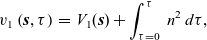 \begin{eqnarray}v_1\left(\boldsymbol{{s}},\tau\right)&=&V_1(\boldsymbol{{s}})+\int_{\tau=0}^\tau\;n^2\;d\tau,\end{eqnarray}
with n describing the relation between the two wave-numbers.
The study of two wave-bearing media gives rise to an entirely new application to the vectorial theory presented here – Navier’s equations of elasticity. It is well known that a wave travelling through an elastic medium and incident upon a boundary gives rise to two types of reflected wave motion – ‘longitudinal’ and ‘shear’, each of which would have their own wave-speed, so each of these would require a generalised Friedlander–Keller ray ansatz of their own. Of course, this is different to the two fields considered in this paper as both electric and magnetic fields have the same wave-speed (the speed of light).
Returning to the electromagnetic case, Maxwell’s equations (2.1) and (2.2) are only valid in a homogeneous media, that is, for constant,
 $O\!\left(1\right)$
scalar quantities
$O\!\left(1\right)$
scalar quantities
 $\epsilon$
and
$\epsilon$
and
 $\mu$
(describing the permittivity and permeability of the medium). If the medium is no longer homogeneous, then equations (2.2) become
$\mu$
(describing the permittivity and permeability of the medium). If the medium is no longer homogeneous, then equations (2.2) become
 \begin{eqnarray}\boldsymbol{\nabla}\boldsymbol{\cdot}\left(\epsilon\boldsymbol{{E}}\right)=0,\ \ \mbox{and}\ \ \boldsymbol{\nabla}\boldsymbol{\cdot}\left(\mu\boldsymbol{{H}}\right)=0,\end{eqnarray}
and the subsequent theory would be different from the start. As the medium is no longer homogeneous, this would change the form of the leading-order exponent term, and this would be another example of solution (4.1) being relevant. In addition to this, and the following exponent terms being different, there would be differences in the subsequent transport equations also, as the various
 $\epsilon$
and
$\epsilon$
and
 $\mu$
terms can no longer be cancelled like they were in the derivations in Section 2. In turn, this motivates the study of generalised Friedlander–Keller ray expansions in which there are corrections to the scalar quantities, for example, if
$\mu$
terms can no longer be cancelled like they were in the derivations in Section 2. In turn, this motivates the study of generalised Friedlander–Keller ray expansions in which there are corrections to the scalar quantities, for example, if
 $\epsilon\sim \epsilon_0+k^{-1/N}\epsilon_1$
, and similarly for
$\epsilon\sim \epsilon_0+k^{-1/N}\epsilon_1$
, and similarly for
 $\mu$
. Such examples may arise in the ‘perturbed’ boundary cases considered by Tew [Reference Tew17, Reference Tew18]. This particular analysis is well underway and will be reported on shortly.
$\mu$
. Such examples may arise in the ‘perturbed’ boundary cases considered by Tew [Reference Tew17, Reference Tew18]. This particular analysis is well underway and will be reported on shortly.
One final extension worthy of mention pertains to the case of waves that do not conform to a time-harmonic form. It was stated that the electric and magnetic fields here assumed (and suppressed) a time-harmonic dependency,
 $e^{-i\omega t}$
. If this assumption were to be removed, so the electric and magnetic fields now take the generic form
$e^{-i\omega t}$
. If this assumption were to be removed, so the electric and magnetic fields now take the generic form
 $\boldsymbol{{E}}\left(\boldsymbol{{x}},t\right)$
and
$\boldsymbol{{E}}\left(\boldsymbol{{x}},t\right)$
and
 $\boldsymbol{{H}}\left(\boldsymbol{{x}},t\right)$
, respectively, then the leading-order exponent term,
$\boldsymbol{{H}}\left(\boldsymbol{{x}},t\right)$
, respectively, then the leading-order exponent term,
 $v_1$
, would no longer satisfy eikonal equation (1.3) . Instead, it would become the time-dependent version:
$v_1$
, would no longer satisfy eikonal equation (1.3) . Instead, it would become the time-dependent version:
 \begin{eqnarray}\boldsymbol{\nabla}v_1\boldsymbol{\cdot}\boldsymbol{\nabla}v_1&=&\left(\frac{\partial v_1}{\partial t}\right)^2.\end{eqnarray}
This aspect would result in a fundamental change to the geometry of the solutions – the first comment on this is that the rays would no longer necessarily be straight lines. This difference (along with any others which may arise) would propagate through and fundamentally change the solution types to
 $v_i$
(for
$v_i$
(for
 $i=2,3,\cdots,N$
) and the transport equations for the electric/magnetic fields. This example, together with all of those mentioned in this section, is currently under investigation and will be reported on separately.
$i=2,3,\cdots,N$
) and the transport equations for the electric/magnetic fields. This example, together with all of those mentioned in this section, is currently under investigation and will be reported on separately.
Acknowledgement
One of the authors (A. M. R. Radjen) is grateful to the University of Nottingham for providing a fully funded Ph.D. scholarship during the course of this research.
Appendix A Derivation of Field Equations
Here, a full derivation of the equations (2.19)–(2.24) is given. It has already been noted that
 $v_1$
satisfies the eikonal equation (1.3), so the first aim is to determine the field partial differential equations for the remaining
$v_1$
satisfies the eikonal equation (1.3), so the first aim is to determine the field partial differential equations for the remaining
 $N-1$
exponent terms. This is done by focusing on the second set of terms in equations (2.15) and (2.16) . The idea is to manipulate these terms so that they appear as a summation of scalars multiplying the electric vectors. For now, the two equations to consider are
$N-1$
exponent terms. This is done by focusing on the second set of terms in equations (2.15) and (2.16) . The idea is to manipulate these terms so that they appear as a summation of scalars multiplying the electric vectors. For now, the two equations to consider are
 \begin{eqnarray}\sum_{n=0}^m\;\left(\boldsymbol{\nabla}v_{m+1-n}{\times}\boldsymbol{{E}}_n\right)-\sqrt{\frac{\mu}{\epsilon}}\boldsymbol{{H}}_m&=&\textbf{0},\end{eqnarray}
 \begin{eqnarray}\sum_{n=0}^m\;\left(\boldsymbol{\nabla}v_{m+1-n}{\times}\boldsymbol{{H}}_n\right)+\sqrt{\frac{\epsilon}{\mu}}\boldsymbol{{E}}_m&=&\textbf{0},\end{eqnarray}
where the m summation limit is valid for
 $m=1,2,\cdots N-1$
. The magnetic fields need to be eliminated between these equations. Firstly, equation (2.18) gives
$m=1,2,\cdots N-1$
. The magnetic fields need to be eliminated between these equations. Firstly, equation (2.18) gives
 $\boldsymbol{{H}}_0$
in terms of
$\boldsymbol{{H}}_0$
in terms of
 $\boldsymbol{{E}}_0$
and
$\boldsymbol{{E}}_0$
and
 $\boldsymbol{\nabla}v_1$
, and expressions for
$\boldsymbol{\nabla}v_1$
, and expressions for
 $\boldsymbol{{H}}_1,\boldsymbol{{H}}_2,\cdots,\boldsymbol{{H}}_{N-1}$
can be obtained from equation (A2). As the m in equation (A1) is valid for
$\boldsymbol{{H}}_1,\boldsymbol{{H}}_2,\cdots,\boldsymbol{{H}}_{N-1}$
can be obtained from equation (A2). As the m in equation (A1) is valid for
 $m=1,2,\cdots,N-1$
, this can be used to express
$m=1,2,\cdots,N-1$
, this can be used to express
 $\boldsymbol{{H}}_1,\boldsymbol{{H}}_2,\cdots,\boldsymbol{{H}}_{N-1}$
in terms of
$\boldsymbol{{H}}_1,\boldsymbol{{H}}_2,\cdots,\boldsymbol{{H}}_{N-1}$
in terms of
 $\boldsymbol{\nabla}v_1,\boldsymbol{\nabla}v_2,\cdots,\boldsymbol{\nabla}v_N$
and
$\boldsymbol{\nabla}v_1,\boldsymbol{\nabla}v_2,\cdots,\boldsymbol{\nabla}v_N$
and
 $\boldsymbol{{E}}_1,\boldsymbol{{E}}_2,\cdots,\boldsymbol{{E}}_{N_1}$
. Doing so, then taking the product
$\boldsymbol{{E}}_1,\boldsymbol{{E}}_2,\cdots,\boldsymbol{{E}}_{N_1}$
. Doing so, then taking the product
 $\boldsymbol{\nabla}v_1{\times}$
(A1)
$\boldsymbol{\nabla}v_1{\times}$
(A1)
 $+\displaystyle{\sqrt{\frac{\mu}{\epsilon}}}$
(A2) gives the one equation
$+\displaystyle{\sqrt{\frac{\mu}{\epsilon}}}$
(A2) gives the one equation
 \begin{eqnarray}\sum_{n=0}^m\;\left[\boldsymbol{\nabla}v_1{\times}\left(\boldsymbol{\nabla}v_{m+1-n}{\times}\boldsymbol{{E}}_n\right)\right]+\boldsymbol{{E}}_m&&\nonumber\\[3pt]+\sum_{n=0}^m\sum_{j=0}^n\;\left[\boldsymbol{\nabla}v_{m+1-n}{\times}\left(\boldsymbol{\nabla}v_{n+1-j}{\times}\boldsymbol{{E}}_j\right)\right]&=&\textbf{0}.\end{eqnarray}
This has entirely decoupled the magnetic field, leaving one equation containing the electric field. Expanding out the various triple vector products in equation (A3) gives
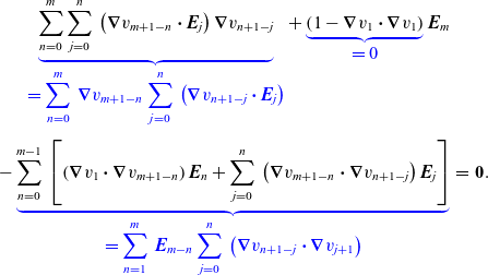
The first comment to make here is that the lowest-order electric field
 $\boldsymbol{{E}}_m$
has now vanished as a result of the eikonal equation (1.3) . Moreover, the two double summations can be combined to give the result
$\boldsymbol{{E}}_m$
has now vanished as a result of the eikonal equation (1.3) . Moreover, the two double summations can be combined to give the result
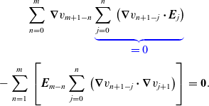
Equation (A5) can be simplified further – the first term contains an inner summation which is scalar and is identical to the second term in divergence equation (2.14) . As a result, the
 $\boldsymbol{\nabla}v_{m+1-n}$
vector is always multiplied by a zero coefficient. Thus, as the various
$\boldsymbol{\nabla}v_{m+1-n}$
vector is always multiplied by a zero coefficient. Thus, as the various
 $\boldsymbol{{E}}_i$
vectors are taken to be non-zero, it follows that the scalar inner summation of the second term of equation (A5) must be zero. Hence,
$\boldsymbol{{E}}_i$
vectors are taken to be non-zero, it follows that the scalar inner summation of the second term of equation (A5) must be zero. Hence,
 $v_2,\cdots,v_{N}$
satisfy the recursive system of partial differential equations given by equation (2.19) .
$v_2,\cdots,v_{N}$
satisfy the recursive system of partial differential equations given by equation (2.19) .
The next group of terms to consider is the final set summations equations (2.15) and (2.16) (i.e. the terms appearing at
 $O\!\left(1\right)$
and lower). The idea is to decouple these two equations and obtain an equation for one single electric vector
$O\!\left(1\right)$
and lower). The idea is to decouple these two equations and obtain an equation for one single electric vector
 $\boldsymbol{{E}}_q$
 $\left(q\ge 0\right)$
. This is done by setting the p index in equations (2.15) and (2.16) to
$\left(q\ge 0\right)$
. This is done by setting the p index in equations (2.15) and (2.16) to
 $p=N+q$
to ensure that all terms appearing in those equations contribute to the sought after transport equation. With this value of p, equations (2.15) and (2.16) become
$p=N+q$
to ensure that all terms appearing in those equations contribute to the sought after transport equation. With this value of p, equations (2.15) and (2.16) become
 \begin{eqnarray}i\sum_{n=1}^N\;\left(\boldsymbol{\nabla}v_{N+1-n}{\times}\boldsymbol{{E}}_{N+n+q}\right)+\left(\boldsymbol{\nabla}{\times}\boldsymbol{{E}}_{N+q}\right)-i\sqrt{\frac{\mu}{\epsilon}}\boldsymbol{{H}}_{2N+q}&=&\textbf{0},\end{eqnarray}
 \begin{eqnarray}i\sum_{n=1}^N\;\left(\boldsymbol{\nabla}v_{N+1-n}{\times}\boldsymbol{{H}}_{N+n+q}\right)+\left(\boldsymbol{\nabla}{\times}\boldsymbol{{H}}_{N+q}\right)+i\sqrt{\frac{\epsilon}{\mu}}\boldsymbol{{E}}_{2N+q}&=&\textbf{0}.\end{eqnarray}
To decouple these two equations, the magnetic field needs to be removed. Fortunately, the third terms in equation (2.15) give a relation between
 $\boldsymbol{{H}}_{N+p}$
in terms of higher-order
$\boldsymbol{{H}}_{N+p}$
in terms of higher-order
 $\boldsymbol{{E}}$
terms and the gradients of the various v functions:
$\boldsymbol{{E}}$
terms and the gradients of the various v functions:
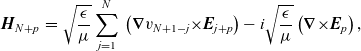 \begin{eqnarray}\boldsymbol{{H}}_{N+p}&=&\sqrt{\frac{\epsilon}{\mu}}\sum_{j=1}^N\;\left(\boldsymbol{\nabla}v_{N+1-j}{\times}\boldsymbol{{E}}_{j+p}\right)-i\sqrt{\frac{\epsilon}{\mu}}\left(\boldsymbol{\nabla}{\times}\boldsymbol{{E}}_p\right),\end{eqnarray}
which equation (2.16) guarantees is valid for
 $p\ge 0$
. Inserting equation (A8) into the first and second terms in equation (A7) (once with
$p\ge 0$
. Inserting equation (A8) into the first and second terms in equation (A7) (once with
 $p=n+q$
and once with
$p=n+q$
and once with
 $p=q$
, respectively) yields an equation containing only electric vectors
$p=q$
, respectively) yields an equation containing only electric vectors
 $\boldsymbol{{E}}_N,\boldsymbol{{E}}_{N+1},\cdots,\boldsymbol{{E}}_{N+q}$
and gradients of the exponent terms. Taking the vector product
$\boldsymbol{{E}}_N,\boldsymbol{{E}}_{N+1},\cdots,\boldsymbol{{E}}_{N+q}$
and gradients of the exponent terms. Taking the vector product
 $\boldsymbol{\nabla}v_1{\times}$
(A6)
$\boldsymbol{\nabla}v_1{\times}$
(A6)
 $+\displaystyle{\sqrt{\frac{\mu}{\epsilon}}}$
(A7) then gives the following single equation:
$+\displaystyle{\sqrt{\frac{\mu}{\epsilon}}}$
(A7) then gives the following single equation:
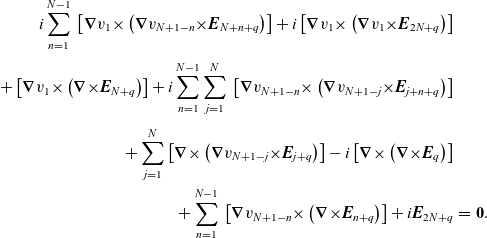 \begin{eqnarray}i\sum_{n=1}^{N-1}\;\left[\boldsymbol{\nabla}v_1{\times}\left(\boldsymbol{\nabla}v_{N+1-n}{\times}\boldsymbol{{E}}_{N+n+q}\right)\right]+i\left[\boldsymbol{\nabla}v_1{\times}\left(\boldsymbol{\nabla}v_1{\times}\boldsymbol{{E}}_{2N+q}\right)\right]&&\nonumber\\[3pt] +\left[\boldsymbol{\nabla}v_1{\times}\left(\boldsymbol{\nabla}{\times}\boldsymbol{{E}}_{N+q}\right)\right]+i\sum_{n=1}^{N-1}\sum_{j=1}^N\;\left[\boldsymbol{\nabla}v_{N+1-n}{\times}\left(\boldsymbol{\nabla}v_{N+1-j}{\times}\boldsymbol{{E}}_{j+n+q}\right)\right]&&\nonumber\\[3pt]+\sum_{j=1}^N\left[\boldsymbol{\nabla}{\times}\left(\boldsymbol{\nabla}v_{N+1-j}{\times}\boldsymbol{{E}}_{j+q}\right)\right]-i\left[\boldsymbol{\nabla}{\times}\left(\boldsymbol{\nabla}{\times}\boldsymbol{{E}}_q\right)\right]&&\nonumber\\+\sum_{n=1}^{N-1}\;\left[\boldsymbol{\nabla}v_{N+1-n}{\times}\left(\boldsymbol{\nabla}{\times}\boldsymbol{{E}}_{n+q}\right)\right]+i\boldsymbol{{E}}_{2N+q}&=&\textbf{0}.\end{eqnarray}
Expanding out the various vector triple products and double summations then gives, in full

The first comment to make here is that an additional set of terms has been added here. As the exponent terms are scalar, it follows by vector calculus that
 $\boldsymbol{\nabla}{\times}\boldsymbol{\nabla}v_n=\textbf{0}$
is always true. This means that the vector triple-product
$\boldsymbol{\nabla}{\times}\boldsymbol{\nabla}v_n=\textbf{0}$
is always true. This means that the vector triple-product
 $\boldsymbol{{E}}_{n+q}{\times}\left(\boldsymbol{\nabla}{\times}\boldsymbol{\nabla}v_{N+q-n}\right)$
can be added N times without invalidating the equality. The purpose of doing so is to allow the vector identity
$\boldsymbol{{E}}_{n+q}{\times}\left(\boldsymbol{\nabla}{\times}\boldsymbol{\nabla}v_{N+q-n}\right)$
can be added N times without invalidating the equality. The purpose of doing so is to allow the vector identity
 \begin{eqnarray}&&\left[\boldsymbol{\nabla}{\times}\left(\boldsymbol{{a}}{\times}\boldsymbol{{b}}\right)\right]+\left[\boldsymbol{{a}}{\times}\left(\boldsymbol{\nabla}{\times}\boldsymbol{{b}}\right)\right]+\left[\boldsymbol{{b}}{\times}\left(\boldsymbol{\nabla}{\times}\boldsymbol{{a}}\right)\right]\nonumber\\&=&-2\!\left(\boldsymbol{{a}}\boldsymbol{\cdot}\boldsymbol{\nabla}\right)\boldsymbol{{b}}-\left(\boldsymbol{\nabla}\boldsymbol{\cdot}\boldsymbol{{a}}\right)\boldsymbol{{b}}+\left(\boldsymbol{\nabla}\boldsymbol{\cdot}\boldsymbol{{b}}\right)\boldsymbol{{a}}+\boldsymbol{\nabla}\left(\boldsymbol{{a}}\boldsymbol{\cdot}\boldsymbol{{b}}\right),\end{eqnarray}
valid for any vectors
 $\boldsymbol{{a}}$
and
$\boldsymbol{{a}}$
and
 $\boldsymbol{{b}}$
to be used. Also, the expanded summations appearing in equation (A10) can be regrouped, so they appear as a single inner summation of scalars multiplying an outer summation of vectors.
$\boldsymbol{{b}}$
to be used. Also, the expanded summations appearing in equation (A10) can be regrouped, so they appear as a single inner summation of scalars multiplying an outer summation of vectors.

Note that the single scalar summation
 $\displaystyle{\sum_{m=0}^n\left(\boldsymbol{\nabla}v_{n+1-m}\boldsymbol{\cdot}\boldsymbol{\nabla}v_{m+1}\right)}$
immediately vanishes as a direct consequence of the ‘exponent’ equations (2.19) (as the upper limit in the summation is
$\displaystyle{\sum_{m=0}^n\left(\boldsymbol{\nabla}v_{n+1-m}\boldsymbol{\cdot}\boldsymbol{\nabla}v_{m+1}\right)}$
immediately vanishes as a direct consequence of the ‘exponent’ equations (2.19) (as the upper limit in the summation is
 $n=1,2,\cdots,N-1$
). Moreover, the final term in divergence equation (2.14) can be used to replace the
$n=1,2,\cdots,N-1$
). Moreover, the final term in divergence equation (2.14) can be used to replace the
 $\boldsymbol{\nabla}\boldsymbol{\cdot}\boldsymbol{{E}}_p$
term, allowing the third summation in equation (A12) to be simplified. Next, the fourth summation in equation (A12) can be simplified by taking the gradient of divergence equation (2.14) . Finally, applying the vector identity
$\boldsymbol{\nabla}\boldsymbol{\cdot}\boldsymbol{{E}}_p$
term, allowing the third summation in equation (A12) to be simplified. Next, the fourth summation in equation (A12) can be simplified by taking the gradient of divergence equation (2.14) . Finally, applying the vector identity
 $\left[\boldsymbol{\nabla}{\times}\left(\boldsymbol{\nabla}{\times}\boldsymbol{{E}}_q\right)\right]=\boldsymbol{\nabla}\left(\boldsymbol{\nabla}\boldsymbol{\cdot}\boldsymbol{{E}}_q\right)-\nabla^2\boldsymbol{{E}}_q$
all yields the sought-after transport equation for each electric vector. The result being equation (2.21) .
$\left[\boldsymbol{\nabla}{\times}\left(\boldsymbol{\nabla}{\times}\boldsymbol{{E}}_q\right)\right]=\boldsymbol{\nabla}\left(\boldsymbol{\nabla}\boldsymbol{\cdot}\boldsymbol{{E}}_q\right)-\nabla^2\boldsymbol{{E}}_q$
all yields the sought-after transport equation for each electric vector. The result being equation (2.21) .


 Open access