


Introduction
Adolescence is a risk period for mental health. The onset of any mental disorder peaks at 14.5 years (Solmi et al., Reference Solmi, Radua, Olivola, Croce, Soardo, Salazar de Pablo, Il Shin, Kirkbride, Jones, Kim, Kim, Carvalho, Seeman, Correll and Fusar-Poli2022), encompassing 25% of the mental disorder burden across their entire lives (Kieling et al., Reference Kieling, Buchweitz, Caye, Silvani, Ameis, Brunoni, Cost, Courtney, Georgiades, Merikangas, Henderson, Polanczyk, Rohde, Salum and Szatmari2024). Globally, the number of adolescents suffering from depression, anxiety and other mental conditions is rising at alarming rates. The prevalence of depression and anxiety was 6% and 3%, respectively, in 2010–13 (Erskine et al., Reference Erskine, Baxter, Patton, Moffitt, Patel, Whiteford and Scott2017), doubled during the COVID-19 pandemic (Racine et al., Reference Racine, McArthur, Cooke, Eirich, Zhu and Madigan2021) and is persistently high (Agency for Healthcare Research and Quality, 2022). Mental health problems can severely disrupt their health and mortality in adolescence and adulthood. In adolescence, 20% of all disease-related disability are attributable to mental disorders (Kieling et al., Reference Kieling, Buchweitz, Caye, Silvani, Ameis, Brunoni, Cost, Courtney, Georgiades, Merikangas, Henderson, Polanczyk, Rohde, Salum and Szatmari2024). Adolescent mental health problems are linked to harmful behaviours such as suicidal attempts, substance misuse and alcohol overconsumption, increasing associated premature death (Yu et al., Reference Yu, Goulter, Godwin and McMahon2023). We are in an urgent need to identify effective interventions to mitigate adolescent mental health problems.
Household poverty is one of the prominent risk factors for mental health problems, with a large body of evidence of the causal associations from natural experiments and randomized trials (Ridley et al., Reference Ridley, Rao, Schilbach and Patel2020). The associations are also reported in adolescents (Dashiff et al., Reference Dashiff, DiMicco, Myers and Sheppard2009; Zaneva et al., Reference Zaneva, Guzman-Holst, Reeves and Bowes2022). Household poverty entails experiences of threat, deprivation and unpredictability (Rakesh et al., Reference Rakesh, Whittle, Sheridan and McLaughlin2023), resulting in worse adolescent mental health via various mechanisms, including physical ill-health, less appropriate parenting, toxic neighbourhood environment, low social status and stigma (Dashiff et al., Reference Dashiff, DiMicco, Myers and Sheppard2009; Ridley et al., Reference Ridley, Rao, Schilbach and Patel2020). Notably, children are disproportionately affected by poverty; around 16% of children in the world experience absolute poverty, which shows an increase due to the COVID-19 pandemic (Salmeron-Gomez et al., Reference Salmeron-Gomez, Engilbertsdottir, Cuesta Leiva, Newhouse and Stewart2023). Even in high-income countries such as Japan, the child poverty rate is 12% (Household Statistics Office, Ministry of Health Labour and Welfare, 2022). Therefore, many children in high-income countries may be at risk of adolescent mental health problems due to poverty. However, randomized trials are predominately conducted in low- and middle-income countries, which target children who are exposed to absolute poverty (Zaneva et al., Reference Zaneva, Guzman-Holst, Reeves and Bowes2022). This sampling bias may make it difficult to generalize the results to children exposed to poverty in high-income countries.
Another important knowledge gap is the effective timing of intervention in childhood poverty. It is reasonable to conceive different effects by the timing of exposure (the timing hypothesis), as the child’s socio-emotional influence of environmental input is uniquely strong when tremendous developmental changes occur, especially in neural architecture and circuits (Knudsen, Reference Knudsen2004). As the brain undergoes significant change during early life (Bethlehem et al., Reference Bethlehem, Seidlitz, White, Vogel, Anderson, Adamson, Adler, Alexopoulos, Anagnostou, Areces-Gonzalez, Astle, Auyeung, Ayub, Bae, Ball, Baron-Cohen, Beare, Bedford, Benegal, Beyer, Blangero, Blesa Cábez, Boardman, Borzage, Bosch-Bayard, Bourke, Calhoun, Chakravarty, Chen, Chertavian, Chetelat, Chong, Cole, Corvin, Costantino, Courchesne, Crivello, Cropley, Crosbie, Crossley, Delarue, Delorme, Desrivieres, Devenyi, Di Biase, Dolan, Donald, Donohoe, Dunlop, Edwards, Elison, Ellis, Elman, Eyler, Fair, Feczko, Fletcher, Fonagy, Franz, Galan-Garcia, Gholipour, Giedd, Gilmore, Glahn, Goodyer, Grant, Groenewold, Gunning, Gur, Gur, Hammill, Hansson, Hedden, Heinz, Henson, Heuer, Hoare, Holla, Holmes, Holt, Huang, Im, Ipser, Jack, Jackowski, Jia, Johnson, Jones, Jones, Kahn, Karlsson, Karlsson, Kawashima, Kelley, Kern, Kim, Kitzbichler, Kremen, Lalonde, Landeau, Lee, Lerch, Lewis, Li, Liao, Liston, Lombardo, Lv, Lynch, Mallard, Marcelis, Markello, Mathias, Mazoyer, McGuire, Meaney, Mechelli, Medic, Misic, Morgan, Mothersill, Nigg, Ong, Ortinau, Ossenkoppele, Ouyang, Palaniyappan, Paly, Pan, Pantelis, Park, Paus, Pausova, Paz-Linares, Pichet Binette, Pierce, Qian, Qiu, Qiu, Raznahan, Rittman, Rodrigue, Rollins, Romero-Garcia, Ronan, Rosenberg, Rowitch, Salum, Satterthwaite, Schaare, Schachar, Schultz, Schumann, Schöll, Sharp, Shinohara, Skoog, Smyser, Sperling, Stein, Stolicyn, Suckling, Sullivan, Taki, Thyreau, Toro, Traut, Tsvetanov, Turk-Browne, Tuulari, Tzourio, Vachon-Presseau, Valdes-Sosa, Valdes-Sosa, Valk, van Amelsvoort, Vandekar, Vasung, Victoria, Villeneuve, Villringer, Vértes, Wagstyl, Wang, Warfield, Warrier, Westman, Westwater, Whalley, Witte, Yang, Yeo, Yun, Zalesky, Zar, Zettergren, Zhou, Ziauddeen, Zugman, Zuo, Bullmore and Alexander-Bloch2022), the particularly strong effect of exposure may lie in early childhood. Seminal research on socio-emotional outcomes of institutionalized children supported the importance of the early childhood environment, suggesting the first 2 years of life as the sensitive period (Gabard-Durnam and McLaughlin, Reference Gabard-Durnam and McLaughlin2020; van Ijzendoorn et al., Reference van Ijzendoorn, Bakermans-Kranenburg, Duschinsky, Fox, Goldman, Gunnar, Johnson, Nelson, Reijman, Skinner, Zeanah and Sonuga-Barke2020). While institutionalization can be a more severe form of adversity than poverty, children in poor households are also exposed to deprivation and threat experiences, implying that poverty in early childhood may uniquely impact a child’s socio-emotional development. Likewise, Heckman’s innovative experimental studies and the following observational studies collectively indicated that financial investment may be most effective in early childhood (Cunha et al., Reference Cunha, Heckman, Lochner, Masterov, Hanushek and Welch2006).
However, the poverty’s timing effects on child and adolescent mental health have been uncertain. A study with repeated measures of poverty during pregnancy, infancy (6 months), early childhood (5 years) and adolescence (14 years) found no evidence for the timing effects after adjusting for poverty at other phases; yet, it suggested the cumulative effect, which was operationalized as the cumulative times experiencing household poverty from pregnancy to adolescence (Najman et al., Reference Najman, Hayatbakhsh, Clavarino, Bor, O’Callaghan and Williams2010b). A study examining the associations between poverty trajectories from early (9 months to 7 years) to late childhood (11–14 years) and problem behaviours at age 14 years identified comparable impacts of poverty in late childhood and chronic poverty (Lai et al., Reference Lai, Wickham, Law, Whitehead, Barr and Taylor-Robinson2019). Another study suggested the cumulative effect of poverty by using mediation analysis (Evans and Cassells, Reference Evans and Cassells2014). A study using a structured life course approach supported this cumulative effect of poverty from ages 0–5, 6–10 to 11–15 years but also implied the sensitive period in early childhood (6–10 years) (Green et al., Reference Green, Stritzel, Smith, Popham and Crosnoe2018). Collectively, it is still unclear whether exposure in early childhood or accumulation of exposure over time is important.
Furthermore, investigating the timing effects needs a more robust study design and statistical method to properly account for confounding. First, the same exposure at an earlier time is a plausible confounder (Schwartz and Glymour, Reference Schwartz and Glymour2023), as past exposure often causes the current exposure. Second, the past outcome is an important time-varying confounder when associations are bidirectional. In the associations between household poverty and adolescent mental health, not only does poverty cause mental health problems among adolescents but also adolescent mental health problems may lead to poverty – adolescent mental health problems may decrease the amount of social, cognitive and financial resources available to parents, ending up in poverty (Ridley et al., Reference Ridley, Rao, Schilbach and Patel2020). Thus, adolescent mental health can be both a confounder and mediator in a longitudinal setting. This exposure-confounder feedback loop or time-varying confounding affected by exposure can produce biased estimation under the conventional regression-adjustment method (Schwartz and Glymour, Reference Schwartz and Glymour2023). We need robust causal inference methods that accommodate time-varying confounders, especially g-methods (Naimi et al., Reference Naimi, Cole and Kennedy2016). Yet, g-methods are underutilized to examine the timing effects.
We aimed to examine the longitudinal associations between household poverty across childhood and adolescent mental health and investigate the timing effects of poverty. To this end, we used the longitudinal Japanese community-based cohort of school-aged children with a total of five repeated assessments of household poverty from grade 1 (ages 6–7 years) to grade 8 (ages 13–14 years) and measures of subsequent mental health status and leveraged a causal inference method. We hypothesized that household poverty was associated with adolescent mental health problems, and this association is stronger in early childhood compared to later childhood.
Methods
Participants
We analysed the data from the longitudinal community-based cohort, the Adachi Health Impact of Living Difficulty (A-CHILD) study (Ochi et al., Reference Ochi, Isumi, Kato, Doi and Fujiwara2021). This study initially recruited all the first-grade children (ages 6–7 years) in 69 public elementary schools in Adachi, Tokyo, Japan. Subsequently, we followed up with children from the second grade (ages 7–8 years) until the eighth grade (ages 13–14 years) biannually. We only included those with at least one measurement of poverty throughout the observation and adolescent mental health outcomes at the end of the study. We ended up with a total of 5,671 children as an analytical sample. This study was approved by the Ethics Committee at the National Center for Child Health and Development (Study ID: 1147) and Tokyo Medical and Dental University (Study ID: M2016-284). Written informed consent was obtained from all caregivers.
Household poverty
Household poverty was measured in a multifaceted way to capture both income level and deprivation experiences via parent-reported questionnaires in grades 1, 2, 4, 6 and 8. First, low income is a household annual income below Japanese yen 3 million, following the national relative poverty line. Caregivers selected categories that best reflected their household’s income for the past year. Second, we measured experiences of economic hardship, including payment difficulty and material deprivation. Payment difficulty is at least one experience of being unable to afford essential costs, including school trips, extracurricular activities, school meals, housing expenses (rent, loans, utilities), phone bills, insurance and transportation fees. Material deprivation is at least one experience of lacking specific household items due to financial constraints, such as educational materials for children, toys, a dedicated study space, appliances (washing machine, rice cooker, vacuum cleaner, microwave), temperature control options (heater, air conditioner), phone access, bathing facilities, individual beds for children and the savings. We defined household poverty as exposure to any experiences of low income, payment difficulty and material deprivation.
Adolescent mental health
Adolescent mental health was assessed at grade 8 using child- and parent-reported questionnaires. This multi-informant approach can increase the robustness by reducing reporting bias. Also, adolescents may display mental health concerns in particular contexts only; thus, parent and self-reports supplement each other (De Los Reyes et al., Reference De Los Reyes, Augenstein, Wang, Thomas, Drabick, Burgers and Rabinowitz2015).
Child-reported outcomes included depression and self-esteem. Depression was assessed using the Patient Health Questionnaire-9 for adolescents (PHQ-A) (Adachi et al., Reference Adachi, Takahashi, Hirota, Shinkawa, Mori, Saito and Nakamura2020; Johnson et al., Reference Johnson, Harris, Spitzer and Williams2002). We obtained the prorated scores when the number of missing items was less than 3 by dividing the sum score of available items by the number of responded items and multiplying it by the total number of items, 9. The Cronbach’s alpha for the current analytical sample was 0.88. Self-esteem was assessed by the 10-item Children’s Perceived Competence Scale, the Japanese version of the Perceived Competence Scale for Children (Harter, Reference Harter1982; Nagai et al., Reference Nagai, Nomura, Nagata, Kaneko and Uemura2018, Reference Nagai, Nomura, Nagata, Ohgi and Iwasa2015). The Cronbach’s alpha for the current analytical sample was 0.88.
Parent-reported outcomes included internalizing and externalizing problems. Caregivers reported child behaviour problems via the Japanese version of the Strength and Difficulties Questionnaire (SDQ), a 25-item questionnaire (Goodman, Reference Goodman1997; Matsuishi et al., Reference Matsuishi, Nagano, Araki, Tanaka, Iwasaki, Yamashita, Nagamitsu, Iizuka, Ohya, Shibuya, Hara, Matsuda, Tsuda and Kakuma2008). Previous research revealed good convergent but poor discriminant validity within internalizing and externalizing second-order subscales, especially among low-risk populations, and using internalizing and externalizing subscales instead of theoretically supported five subscales is advantageous (Goodman et al., Reference Goodman, Lamping and Ploubidis2010). Therefore, we calculated scores for internalizing (consisting of emotional symptoms and peer relationship problems) and externalizing (consisting of conduct problems and hyperactivity/inattention problems) subscales. Cronbach’s alpha for the current analytical sample were 0.73 and 0.75, respectively.
Covariates
Parent-reported questionnaires assessed various time-varying covariates from grades 1 to 8 and time-invariant covariates at baseline (grade 1). Time-varying covariates included the caregiver’s psychological distress measured with the Kessler Psychological Distress Scale (Furukawa et al., Reference Furukawa, Kawakami, Saitoh, Ono, Nakane, Nakamura, Tachimori, Iwata, Uda, Nakane, Watanabe, Naganuma, Hata, Kobayashi, Miyake, Takeshima and Kikkawa2008; Kessler et al., Reference Kessler, Andrews, Colpe, Hiripi, Mroczek, Normand, Walters and Zaslavsky2002), family size, marital status and child internalizing and externalizing problems measured with SDQ. Time-invariant covariates included child age, child’s biological sex (obtained at a school health checkup), maternal and paternal ages, and household education level. Missing exposures and covariates were imputed using multiple imputations by chained equations (van Buuren S and Groothuis-Oudshoorn, Reference van Buuren S and Groothuis-Oudshoorn2010) including all the exposure, outcome and covariates measures as well as auxiliary variables at all waves (child maltreatment, parent–child interaction, employment status and school dummy) in the imputation model. Imputations were conducted using a predictive mean matching algorithm with a maximum of 25 iterations, producing a total of 30 imputed datasets.
Statistical analysis
We employed g-estimation of structural nested mean modelling using the R package ‘gesttools’ (Keen et al., Reference Keen, Chen, Slopen, Sandel, Copeland and Tiemeier2024; Tompsett et al., Reference Tompsett, Vansteelandt, Dukes and De Stavola2022) to examine the longitudinal associations between household poverty and adolescent mental health (the hypothesized cause-and-effect relationship is mapped out with Directed Acyclic Graph, DAG in Fig. 1). The details can be found in S Text 1. Briefly, g-estimation is a causal inference method that uses a counterfactual framework and can accommodate time-varying confounders. G-estimation can provide unbiased estimates for causal associations when models are correctly specified and the identifiability assumption holds. In the current outcome models, we adjusted for time-invariant covariates, lagged time-varying exposure and covariates, and time-varying propensity scores for being exposed to poverty, weighting for the probability of having poverty measures at each time point. A time-varying propensity score was estimated by regressing poverty at a given age on time-invariant covariates and lagged time-varying covariates and poverty status. Including propensity score in the outcome model helps decrease the influence of residual confounding and model misspecification via doubly robust estimation. Estimates were obtained for each imputed dataset using bootstrapping with 1,000 draws to obtain unbiased standard errors and aggregated across datasets using Rubin’s rule (Rubin, Reference Rubin1987).

Figure 1. Hypothesized longitudinal causal associations between household poverty and mental health. A directed acyclic graph in the current analysis is shown. Arrows in blue indicate associations of interest in the current study and thus were aimed to estimate causal associations. Arrows going back and forth between household poverty and confounders over time suggest the existence of exposure-confounder feedback loops or time-varying confounders. This graph informs us that adjusting confounders at grades 1–4 in the conventional regression-adjustment methods to estimate the joint effects of poverty at grades 2–8 may lead to biased estimation by adjusting for intermediate variables and/or by introducing collider stratification bias in the presence of exposure-confounder feedback loops.
As sensitivity analyses, first, we examined the associations of standardized household income to consider economic inflation over time (S Table 1) and a continuous income measure. Second, we calculated e-values to check the robustness of findings in the face of unmeasured confounding (Mathur et al., Reference Mathur, Ding, Riddell and VanderWeele2018). All the analyses were conducted with the R version 4.3.2 (R core Team, 2023).
Results
Among 5,671 children included in the current analysis, 38% (n = 2,156) of children experienced poverty at any timing throughout the observation. The baseline characteristics who never experienced household poverty (‘never poverty’) and did experience (‘any poverty’) were significantly different in most of the demographic factors and child behaviour problem scores (Table 1). ‘Never poverty’ households had lower socio-economic status and worse mental health for both caregivers and children compared to ‘any poverty’ households. For example, the paternal highest education is junior high school for 4.8% of ‘never poverty’ children and 17.7% of ‘any poverty’ children, while university or higher levels for 49.5% of ‘never poverty’ children and 22.8% of ‘any poverty’ children. Caregiver’s psychological distress scores were 2.7 (SD: 3.5) and 4.7 (SD: 5.1) respectively. The prevalence of child poverty ranged from 22% to 28% across childhood, with some of them having unstable poverty statuses (Fig. 2).

Figure 2. Transition of household poverty status over time. Orange flows indicate children not exposed to household poverty and blue flows indicate children exposed to household poverty. Percentages in bar charts show the prevalence of children exposed/not exposed to household poverty at each grade among the analytical sample.
Table 1. Sample baseline characteristics

Sample characteristics were compared using Welch’s two-sample t-test for continuous values, Pearson’s chi-squared test for parental education, and Pearson’s chi-squared test with Yates’ continuity correction for child sex and marital status.
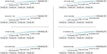
Longitudinal associations between household poverty in childhood and adolescent mental health are shown in Table 2. By properly accounting for time-varying confounders with g-estimation, associations between childhood poverty and adolescent mental health were carefully estimated. On average, adolescents exposed to household poverty at any timing from grades 2 to 8 reported higher levels of depressive symptoms (ψ = 0.32, [95% CI: 0.13; 0.51]) and lower levels of self-esteem (ψ = −0.41, [95% CI: −0.62; −0.21]). Similarly, parents in poor households rated their children as having more internalizing (ψ = 0.19, [95% CI: 0.10; 0.29]) and externalizing (ψ = 0.10, [95% CI: 0.002; 0.19]) problems in adolescence. Further, the effects of the timing of poverty were examined. Household poverty at specific timing was not associated with any adolescent mental health outcomes. Effect size differences, however, indicated potential sensitive periods in earlier childhood compared to later. Adolescents exposed to household poverty in grade 2 (ψ = 0.54, [95% CI: −0.12; 1.19]) showed more depressive symptoms compared to those exposed to poverty in grade 8 (ψ = −0.01, [95% CI: −0.66; 0.64]). Likewise, effect sizes of the associations of household poverty with self-esteem were stronger when exposed in grade 2 (ψ = −0.76, [95% CI: −1.58; 0.05]) compared to in grade 8 (ψ = −0.20, [95% CI: −0.86; 0.45]). However, this trend was not clear for internalizing and externalizing problems. The results are summarized in Fig. 3.

Figure 3. Associations between childhood household poverty and adolescent mental health outcomes. The results of g-estimation of structural nested mean modelling that examines the average of the average treatment effects of household poverty at any grade on mental health outcomes at grade 8 (the upper rows) and age-specific average treatment effects of household poverty at a particular grade on mental health outcomes at grade 8 (the lower rows) are shown. The straight lines indicate statistically significant paths, and the dashed lines indicate statistically non-significant paths.
Table 2. Associations between household poverty in childhood and adolescent mental health

Depression scores range from 0 to 27, with higher scores indicating severe symptoms. Self-esteem scores range from 0 to 30, with higher scores indicating higher levels of self-esteem. Internalizing and externalizing problems scores range from 0 to 20, with higher scores indicating more behavioural problems.
G2 corresponds to ages 7–8 years, G4 ages 9–10 years, G6 ages 11–12 years and G8 ages 13–14 years.
Models adjusted for the past poverty status, time-invariant confounders (child age and sex, maternal and paternal age, and household education level at baseline), time-varying confounders (caregiver’s psychological distress, family size, marital status and child behavioural problems) and propensity score for the current poverty status.
We found similar directions and patterns of the associations of continuous standardized household income (S Table 2), where only the average effects of standardized household income at any childhood age were observed. The e-values are shown in S Table 3. Based on the list of confounders in the main analysis and the magnitude of the associations, unmeasured confounders are unlikely to explain away the observed associations.
Discussion
This is the first longitudinal study that examined the associations between household poverty and adolescent mental health outcomes, focusing on the timing of exposure using a causal inference method, a g-estimation of structural nested mean modelling. We found that household poverty at any age in childhood was averagely associated with worse adolescent mental health – higher levels of depression, lower levels of self-esteem and more behavioural problems. However, we could not find any significant associations of exposure at a specific age. Our findings imply that the effects of household poverty across childhood are not significantly different by the timing of exposure and suggest the cumulative rather than the timing effects.
We found the average effects of childhood household poverty on adolescent mental health. Previous studies consistently demonstrated that household poverty was associated with mental health throughout the lifespan (Ridley et al., Reference Ridley, Rao, Schilbach and Patel2020; Zaneva et al., Reference Zaneva, Guzman-Holst, Reeves and Bowes2022). A meta-analysis of randomized trials of poverty mitigation programmes revealed significantly decreased adolescent mental health problems in response to monetary support (Zaneva et al., Reference Zaneva, Guzman-Holst, Reeves and Bowes2022). However, these randomized trials were mainly conducted in low- and middle-income countries, and studies in high-income countries were mostly observational (Victora et al., Reference Victora, Hartwig, Vidaletti, Martorell, Osmond, Richter, Stein, Barros, Adair, Barros, Bhargava, Horta, Kroker-Lobos, Lee, Menezes, Murray, Norris, Sachdev, Stein, Varghese, Bhutta and Black2022; Zaneva et al., Reference Zaneva, Guzman-Holst, Reeves and Bowes2022). Recently, to establish the causal associations between monetary intervention and child healthy development, a randomized trial of unconditional cash transfer to poor mother–child dyads was launched in the US in 2018 (Noble et al., Reference Noble, Magnuson, Gennetian, Duncan, Yoshikawa, Fox and Halpern-Meekin2021). The intervention up to the first three years of the child’s life brought no differences in the child’s lifestyle and health outcomes between low- and high-cash gift receivers, suggesting the impacts of poverty mitigation might not be visible until later in life (Sperber et al., Reference Sperber, Gennetian, Hart, Kunin-Batson, Magnuson, Duncan, Yoshikawa, Fox, Halpern-Meekin and Noble2023). While a randomized trial is a strong framework to explore the causality, ethical considerations, intervention costs and sampling bias are major limitations (Noble et al., Reference Noble, Magnuson, Gennetian, Duncan, Yoshikawa, Fox and Halpern-Meekin2021; Stuart et al., Reference Stuart, Bradshaw and Leaf2015). Observational studies are often sources of associational evidence but can be likened to randomized trials by using the appropriate statistical approach (Naimi et al., Reference Naimi, Cole and Kennedy2016). Moreover, causal inference approaches utilizing the counterfactual framework can inform the most effective interventions by considering the situation under hypothetical interventions. Our results revealed that if all children were moved from poverty to a non-poverty family environment at any age from 6 to 14 years, at 14 years, their mental health would be improved with reductions in depressive symptoms and behaviour problems and an increase in self-esteem. Although generalizing the findings needs caution, our results suggest the poverty mitigation programme targeting poor households with elementary-school-aged children in high-income countries.
Our findings did not find any childhood age demonstrating statistically significant effects, failing to support the timing hypothesis. So far, several analytical approaches have been taken to test the timing hypothesis. The most conventional approach is to compare the associations of several timings of poverty (i.e., prenatal, infancy, early childhood and adolescence) using a standard regression-adjustment model. This approach found no sensitive periods for internalizing and externalizing problems; rather, it suggested cumulative effects, which were examined as the effects of the number of times being in poverty (Najman et al., Reference Najman, Clavarino, McGee, Bor, Williams and Hayatbakhsh2010a, Reference Najman, Hayatbakhsh, Clavarino, Bor, O’Callaghan and Williams2010b). Another study examining cumulative risk with mediation analysis found the cumulative effects of poverty in childhood (Evans and Cassells, Reference Evans and Cassells2014). Studies exploiting poverty status trajectories during childhood suggested recency effects, i.e., children who experienced the transition into poverty at a later timing and who were exposed to chronic poverty were impacted most strongly (Bøe et al., Reference Bøe, Skogen, Sivertsen, Hysing, Petrie, Dearing and Zachrisson2017; Lai et al., Reference Lai, Wickham, Law, Whitehead, Barr and Taylor-Robinson2019; Pryor et al., Reference Pryor, Strandberg-Larsen, Nybo Andersen, Hulvej Rod and Melchior2019). A structured life-course modelling approach is a theory-based statistical framework that systematically tests multiple life-course models, including sensitive periods (effects of exposure at a specific time point) and accumulation (effects of a sum of times being exposed) (Mishra et al., Reference Mishra, Nitsch, Black, De Stavola, Kuh and Hardy2009; Smith and Dunn, Reference Smith and Dunn2022). Studies using this approach supported the cumulative effects of poverty on general health and externalizing problems in children (Green et al., Reference Green, Stritzel, Smith, Popham and Crosnoe2018; Mazza et al., Reference Mazza, Lambert, Zunzunegui, Tremblay, Boivin and Côté2017). Our causal inference approach is advantageous over these previous approaches in accommodating time-varying confounders (Schwartz and Glymour, Reference Schwartz and Glymour2023).
Importantly, the average effect of household poverty and the lack of evidence of the age-specific effects implied the cumulative rather than the timing effect. Our average effect is not operationalized to indicate the cumulative effect defined in the life-course model, which assessed the dose-response associations of the number of times being in poverty. However, our average effect indicated the significant effect of living in poverty at any childhood age; thus, if children spent more time in poor households, they may show more mental health problems. We confirmed dose–response associations between times being exposed to household poverty and adolescent mental health outcomes using a conventional linear regression approach (S Table 4), where we observed worse mental health among adolescents who were exposed to poverty for longer periods. Biological mechanisms may underlie this potential cumulative effect. Allostatic loads, or physiological damages due to forced adjustment to chronic stress, might partly underlie (Juster et al., Reference Juster, McEwen and Lupien2010). Initially, the body responses to acute stress exposure by adjusting the neural and neuroendocrine systems to maintain stability (allostasis or homeostasis through change), yet extended stress disrupts adjustment abilities (Juster et al., Reference Juster, McEwen and Lupien2010). Another, but not mutually exclusive, explanation is the sensitization model, where the initial stress predisposes the body to subsequent stress exposures, making the later stress a fatal attack (Harkness et al., Reference Harkness, Hayden and Lopez-Duran2015). Understanding the underlying mechanisms essentially requires earlier exposure measurements, as we cannot eliminate the impacts of foetal programming and early-life exposures. Future longitudinal studies should follow up from foetal life onward and repeatedly assess exposures comparably. Furthermore, our results implied that whenever we intervene in household poverty, the negative impacts on adolescent mental health can be alleviated.
While any timing of exposure was not statistically significantly associated, we note that our findings are inconclusive and need further replications. Specifically, earlier-life exposure to adversities can theoretically impact developmental outcomes more strongly (Ho and King, Reference Ho and King2021), and point estimates of earlier exposure were larger than those of the average effects for depression and self-esteem, indicating possible stronger effects of earlier poverty. While the wide-ranged confidence intervals did not support the timing hypothesis, timing effect estimation was basically underpowered compared to the average effect estimation.
Markedly, although we utilized the state-of-the-art causal inference method that leverages a counterfactual framework, the following limitations may prevent us from drawing a strong causal conclusion. First, household income and economic hardship were self-reported. People might not be willing to report actual household income and economic hardship experiences, making extremely high or low income less likely in analytical samples. Recall bias might also be possible. Yet our closed-ended questionnaire may reduce these biases compared to the open-ended form. Future studies should desirably use registry data linked with tax payments. Second, we did not know the participants’ poverty status in early childhood. Although we adjusted for past exposure to poverty as time-varying confounders, this missing information can be an important residual confounder. Future studies should consider a longer period of exposure assessments, including perinatal periods, when a child undergoes tremendous growth thus, a sensitive period might lie. Third, we lacked repeated child-report outcome measures. Considering the bidirectionality between household poverty and child mental health (Ridley et al., Reference Ridley, Rao, Schilbach and Patel2020), we adjusted for parent-report behavioural problems as a time-varying confounder. This time-varying nature would pose further challenges for longitudinal studies that cover formative periods, as transitions between developmental periods may involve changes in mental health measurements and constructs (Murray et al., Reference Murray, Obsuth, Eisner and Ribeaud2019). For example, the Child Behavior Checklist, a widely used questionnaire of emotional and behavioural problems, has separate versions for preschoolers and schoolers, which include different syndrome and clinical diagnostic scales (Maust et al., Reference Maust, Cristancho, Gray, Rushing, Tjoa and Thase2012). Also, there was only a weak but not strong measurement invariance in the emotional subscale of the SDQ (Riglin et al., Reference Riglin, Dennison, Martin, Tseliou, Armitage, Shakeshaft, Heron, Tilling, Thapar and Collishaw2024). We might benefit from using multiple informants by capturing the different contexts and providing deeper and holistic views of a child’s mental health status (De Los Reyes et al., Reference De Los Reyes, Augenstein, Wang, Thomas, Drabick, Burgers and Rabinowitz2015). Fourth, we need caution to generalize the findings outside the current sample, as the participants reside in Adachi, where the proportion of public aid receivers was highest in Tokyo (Tokyo is relatively affluent than other areas in Japan) when the baseline survey was conducted (Ochi et al., Reference Ochi, Isumi, Kato, Doi and Fujiwara2021). Yet, poverty is common worldwide, and biological mechanisms of the psychopathological consequences of poverty should be shared across societies. Thus, some degrees of generalizability may exist. Fifth, we excluded those with no measures of poverty and mental health outcomes, which may introduce further sampling bias. While we were committed to mitigating the sampling bias by imputing variables, utilizing registry data that contain nationally representative income data may further reduce sampling bias.
Conclusions
In conclusion, we found the average effect of household poverty in childhood on adolescent mental health problems. Furthermore, our estimates implied no age-specific effects. These findings indicate that we could mitigate the negative impacts of household poverty at any timing throughout childhood by intervening in households with low-income or economic hardship experiences. Moreover, possible cumulative effects emphasize the benefit of continuous support for those in poverty from early childhood onward. Future studies should properly address time-varying variables, include larger participants, follow up for a longer period and better assess household income to inform effective anti-poverty interventions for improving adolescent mental health.
Supplementary material
The supplementary material for this article can be found at https://doi.org/10.1017/S2045796025000162.
Availability of data and materials
The data and code used for the analysis are not publicly available due to ethical concerns. However, upon reasonable request to the corresponding author, access to the data and code will be provided.
Acknowledgements
We are grateful to the staff members and central office of Adachi City Hall for conducting the survey. Particularly, we thank Mayor Yayoi Kondo, Syuichiro Akiu, Hideaki Otaka, and Yuko Baba of Adachi City Hall, all of whom contributed significantly to the completion of this study.
Financial support
This study was supported by a Health Labour Sciences Research Grant, Comprehensive Research on Lifestyle Disease from the Japanese Ministry of Health, Labour and Welfare (H27-Jyunkankito-ippan-002), Research of Policy Planning and Evaluation from the Japanese Ministry of Health, Labour and Welfare (H29-Seisaku-Shitei-004), Innovative Research Program on Suicide Countermeasures (IRPSC), and Grants-in-Aid for Scientific Research from the Japan Society for the Promotion of Science (JSPS KAKENHI Grant Number 16H03276, 16 K21669, 17 J05974, 17 K13245, 19 K19310, 19 K14029, 19 K19309, 19 K20109, 19 K14172, 19 J01614, 19H04879, 20 K13945, and 21H04848), St. Luke’s Life Science Institute Grants, the Japan Health Foundation Grants, and Research-Aid (Designated Theme), Meiji Yasuda Life Foundation of Health and Welfare. The funder had no role in study design, data collection and analysis, decision to publish, or manuscript preparation.
Competing interests
There is no conflict of interest to declare.
Ethical standards
This study was approved by the Ethics Committee at the National Center for Child Health and Development (Study ID: 1147) and Tokyo Medical and Dental University (Study ID: M2016-284) and complied with the Helsinki Declaration. Written informed consent was obtained from all caregivers.


 Open access