INTRODUCTION
Many common infections like gastrointestinal infections, respiratory infections, malaria and the symptoms associated with these diseases (e.g. diarrhoea, fever, cough, or rapid breathing) occur in recurrent episodes. Disease recurrence and disease clustering in individuals, as well as other characteristics of disease distribution typical for recurrent infections such as seasonality and autocorrelation of subsequent episodes within individuals, have implications for sampling strategies [Reference Schmidt1] and data analysis [Reference Kelly and Lim2]. Disease recurrence can also make it difficult to distinguish between episodes separated by only a few days, especially in settings with high disease incidence [Reference Morris3].
Mathematical models have been used to gain insight into these methodological issues, e.g. to evaluate different disease definitions and sampling strategies. Morris et al. [Reference Morris3] used a simple empirical model to determine the expected distribution of diarrhoea episodes and gaps between episodes. Schmidt et al. [Reference Schmidt1] used a similar model to test different sampling intervals to measure diarrhoea in longitudinal studies.
These empirical models served to generate simulated datasets reflecting the stochastic processes that give rise to the data collected in field studies. In contrast to classic transmission models, such as deterministic compartmental models, these empirical models rarely aim at exploring disease transmission between individuals or the effect of interventions. However, they can be helpful in improving epidemiological methods and tools. The models used previously have been very simple and relied on assumptions that may not be appropriate in certain situations [Reference Schmidt1, Reference Morris3]. For example, they assumed independence between episodes of the same individual (absence of autocorrelation), and no correlation between the number of episodes in an individual and episode duration [Reference Schmidt1, Reference Morris3]. This paper proposes a more flexible model which allows a better description of the stochastic processes that underpin the field data from longitudinal studies of common recurrent diseases. The model can therefore be used to further understanding of the epidemiology of diarrhoea and other episodic diseases, help with the planning of epidemiological studies and programme evaluation, and to compare different statistical methods for data analysis.
BASIC STRUCTURE OF THE MODEL
Our empirical model is based on a concept developed by Morris et al. [Reference Morris3] and represents the daily experience of recurrent infections of a large number of individuals over a specified period of time. The number of diarrhoea episodes in an individual is drawn from a gamma distribution, a distribution suitable to represent skewed random variables [Reference Morris3].
The duration of these episodes (usually also highly skewed) is drawn from a different gamma distribution. Gamma distributions are commonly specified by two parameters: α, the shape parameter and β, the stretch parameter. By varying these two parameters, the simulated data can be made to fit (in the least-squares sense) a wide range of empirical distributions observed in the field.
Similar to previous models, our basic model assumes independence between the number of episodes in an individual and the duration of episodes, and between successive episodes in an individual (i.e. no autocorrelation). The basic model also assumes a constant risk for each individual without seasonal variation. Thus, disease occurrence is specified by only two determinants, each depending on the respective α and β parameters of the specified gamma distributions: (1) the distribution of the number of episodes per individual in the population and (2) the distribution of the durations of these episodes. In further model developments we introduced as additional epidemiological characteristics the dependence of disease occurrence on (3) a correlation between the individual number of episodes and episode duration, (4) previous episodes in an individual (autocorrelation) and (5) seasonality. The parameters of the gamma distributions were fitted to the distributions observed in the field by minimizing the least-squared differences (Excel Solver tool). An outline of the model structure is shown in the Appendix. We implemented the model in Stata version 9.0 (Stata Corp., College Station, TX, USA). The Stata program for the model can be obtained from the authors.
MODEL PARAMETERIZATION
The model was parameterized based on parameter estimates derived from real datasets from field studies conducted in Guatemala, Brazil (2 datasets) and Ghana. The Guatemala data [Reference Reller4] (diarrhoea only) came from a randomized controlled trial of household water treatment (number of study individuals n=1839). One diarrhoea dataset from Brazil (subsequently designated Brazil 1) was collected during a large cohort study in Salvador de Bahia (n=1880) [Reference Strina5], the other (Brazil 2) came from a vitamin A trial in rural northeastern Brazil in a child population with poor nutritional status (n=1180) [Reference Barreto6]. This dataset contains information on diarrhoea, cough and fever. Finally, we included data from the VAST trial in Ghana which was also conducted in a malnourished child population and contains among other conditions data on diarrhoea, rapid breathing (as a sign of lower respiratory infections) and cough (n=1918) [7].
We estimated the distribution of the number of episodes and episode duration from the four real datasets assuming that a new episode started after at least two disease-free days. Only study participants with more than 200 days of observation were included for the parameter estimation. Due to different follow-up times between individuals we calculated the number of episodes as the incidence per 365 days of observation.
In addition, we estimated parameters based on published data. These were restricted to diarrhoea and purposively chosen to cover a broad range of settings. In the following sections we describe the parameterization of the five key characteristics of disease distribution in the model outlined above.
Distribution of number of episodes
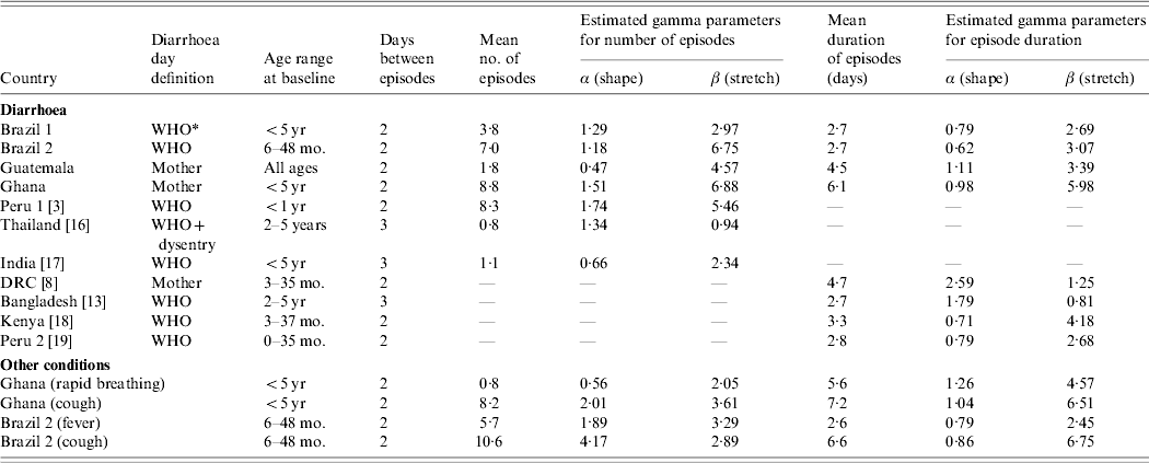
Episodes of many conditions are usually highly clustered in individuals. Figure 1 shows examples of histograms for the distribution of the number of episodes experienced by individuals over 1 year. Each graph contains the observed distribution and the best-fitted gamma distribution. The data show a broad range of distributions. While in Guatemala and Thailand the majority of individuals escaped illness altogether, <7% did so in Ghana and Peru (Fig. 1). The shape of the distribution and the mean number of episodes is likely to be influenced by many factors such as age, study setting, nutritional status and study procedures. The parameter estimation based on the data is summarized in Table 1.

Fig. 1. Distribution of the number of episodes per individual in different settings.■, Observed distributions; □, fitted gamma distributions.
Table 1. Characteristics of the distribution of the number per individual and the duration of episodes
DRC, Democratic Republic of Congo.
* More than 2 loose stools/24 h.
In the model, the number of episodes in an individual is drawn from a gamma distribution with parameters α and β that are estimated from the empirical distributions (Table 1). Previous models have allowed episodes to overlap [Reference Schmidt1, Reference Morris3]. Since overlap increases the duration of episodes and decreases the incidence, it is more appropriate not to allow overlap between episodes, unless overlap is of particular interest [Reference Morris3]. However, the model can be specified either way.
Distribution of illness duration
There are also large differences in the distribution of the episode durations. As shown in Figure 2, episodes lasting for just 1 day predominated in all settings except in a study on children aged <3 years in the Democratic Republic of Congo (DRC) [Reference Haggerty8]. As with incidence, there are likely to be many factors like age and nutritional status affecting episode duration. The data for diarrhoea and cough from Ghana reveal a conspicuous ‘heaping’ of episodes lasting for 7, 14 or 21 days (Fig. 2). It appears that field workers or study participants rounded the episode duration to full weeks. These outliers compromise the parameter estimation for episode durations.
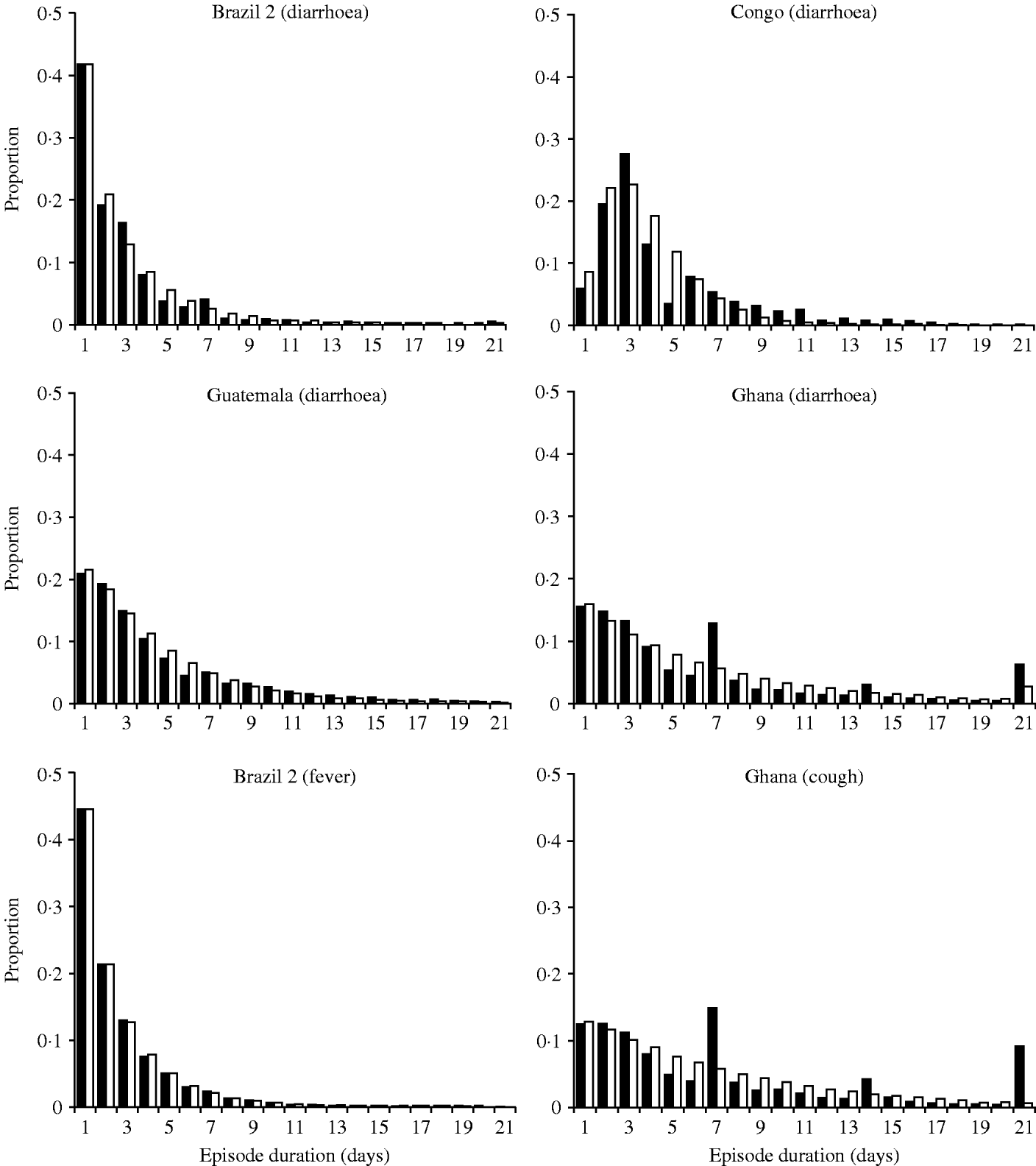
Fig. 2. Distribution of the episode duration in different settings.■, Observed distributions; □, fitted gamma distributions.
In the model, the duration of each diarrhoea episode is drawn from the gamma distribution fitted to the real data, in a way similar to the generation of episode incidence (see Appendix). While we estimated the distribution of the number of episodes at individual level, the estimation of the distribution of the episode durations was episode based, i.e. episodes of all individuals were pooled and then stratified according to their duration regardless of whether some individuals consistently experience longer or shorter episodes. Without further assumptions (see next section) the model randomly allocates episode durations directly to episodes rather than individuals. Thus, the model at this stage ignores the possibility that some individuals may be prone to short or long episodes due to known or unknown risk factors.
Correlation between the individual disease incidence and individual mean episode duration
While in the basic model the episode duration is allocated to each episode at random, this simplified assumption may not reflect reality. The analysis of the available data demonstrated that for conditions like diarrhoea, fever and rapid breathing, individuals with more episodes also suffer from longer episodes (Table 2), presumably due to the effect of age (younger individuals having more and longer episodes) and an underlying nutrient and immune deficiency.
Table 2. The correlation between the number of episodes and episode duration
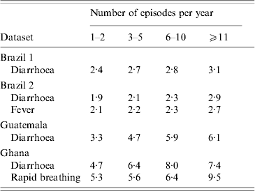
Duration of episodes in days.
The correlation between the number and duration of episodes can be simulated by introducing a linear association between the number of episodes and episode duration, while keeping the mean episode duration as determined by the gamma distribution constant (more complex associations are also possible, but are often not needed). However, comparison of the model simulations and data from the different field sites showed that the association between incidence and duration only partially explained the variation in the mean episode duration between individuals. There was evidence for considerable within-subject correlation of episode duration, with individuals consistently experiencing longer or shorter episodes due to some unknown risk factor unrelated to disease frequency. This intra-subject correlation of episode duration can be incorporated into the model by adding a subject-specific error factor drawn from a normal distribution with mean 1·0. The variance of the normal distribution is increased incrementally until the simulated variance of the mean episode duration between individuals is close to the observed data (see Appendix).
For example, the mean episode duration in the data from Brazil 2 was 2·7 days with a standard deviation of 1·4 days between individuals. In a simulation model based on the parameters from Brazil 2 (Table 1), the mean duration was also 2·7 days. However, without specifying an error factor to account for within-subject correlation of episode duration, the standard deviation of episode durations was only 0·8 days – much lower than observed in the real data. Specifying an error term drawn from a normal distribution with mean 1·0 and variance 0·5 results in a standard deviation of 1·4 between individuals as was observed in the real data. The same approach applied to the other datasets revealed similar values for the variance of the error term: for the Ghana data, the error factor with the best fit had variance of 0·6, in Guatemala of 0·4 (mean 1·0). To illustrate the procedure, Figure 3 shows the association between the number of episodes and the mean duration of episodes in individuals in the data from Brazil 2 (Fig. 3 a), and in the model incorporating a linear association between incidence and duration, as well as within-subject correlation of episode duration, which increases the scatter around the regression line (Fig. 3 b).
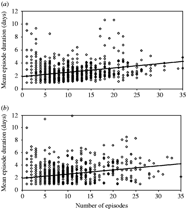
Fig. 3. Correlation between incidence and episode duration: (a) data; (b) model. Diamonds indicate the mean episode duration of individuals according to individual incidence (n=1000). The line indicates the regression line.
Dependence of disease risk on the occurrence of previous episodes (autocorrelation)
As outlined above, specifying a gamma distribution for the individual number of episodes without further assumptions leads to episodes being randomly distributed over time. However, two different populations with the same gamma distribution of the number of episodes may well differ with regard to how these episodes are spread over time, e.g. due to seasonal variation (see next section) or autocorrelation. There is evidence that the risk of a new diarrhoea episode depends on the occurrence of previous episodes [Reference Genser9, Reference Lima10]. The analysis of the available datasets suggests that diarrhoea risk decreased by 50% 4–6 weeks after a previous episode in Brazil 1 (Fig. 4). The diarrhoea data from Ghana and Brazil 2 showed a very similar pattern (results not shown). A dependence of the risk on the time since the last episode was also found for the rapid breathing data from Ghana, and to a lesser extent also for fever in Brazil 2 (Fig. 4). In contrast, the diarrhoea data from Guatemala revealed no clear autocorrelation (results not shown). Overall, the risk of some recurrent infections and conditions appears to level off beyond 4 weeks after the last episode. However, the estimated association also depends on the number of disease-free days assumed to define a new episode. Some episodes occurring in the week after a first episode may belong to the previous one. It is therefore possible that the true association between disease risk and the time since last episode has been overestimated but is unlikely to have been underestimated.
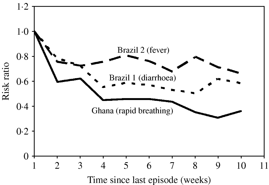
Fig. 4. Disease risk as a function of time elapsed since the last episode. We used binomial regression (log risk) with week 1 after an episode as reference, adjusted for individual incidence rate and seasonal variation.
There are many ways to incorporate into the model a dependency of disease risk on previous episodes. The available data suggest that a negative exponential association between risk and time since last episode may be appropriate. Alternatively, one can simulate discrete steps, e.g. by assuming that the risk of disease is uniformly increased for a defined period after an episode, after which the risk drops to the original risk. As with all models there are trade-offs between using simple assumptions that may not fit the data as well and increasing the complexity of the model.
Seasonality
Diarrhoea and many other recurrent infectious diseases and conditions like malaria-associated fever or respiratory infections are known to strongly depend on season. In most settings, diarrhoea and malaria increase over the wet season, whereas respiratory infections often peak during the cold or dry season. In some regions there is a second peak of diarrhoea in the cold season (as shown in Fig. 5 for Ghana). In contrast to Brazil 2 the peak of respiratory infections seems to coincide with the peak of diarrhoea during summer (Fig. 5). Whereas in the data from Brazil 2 diarrhoea and cough follow a gradual rise and decline, the seasonality in the Ghana study is characterized by a relatively constant baseline risk, interrupted by sudden epidemics.
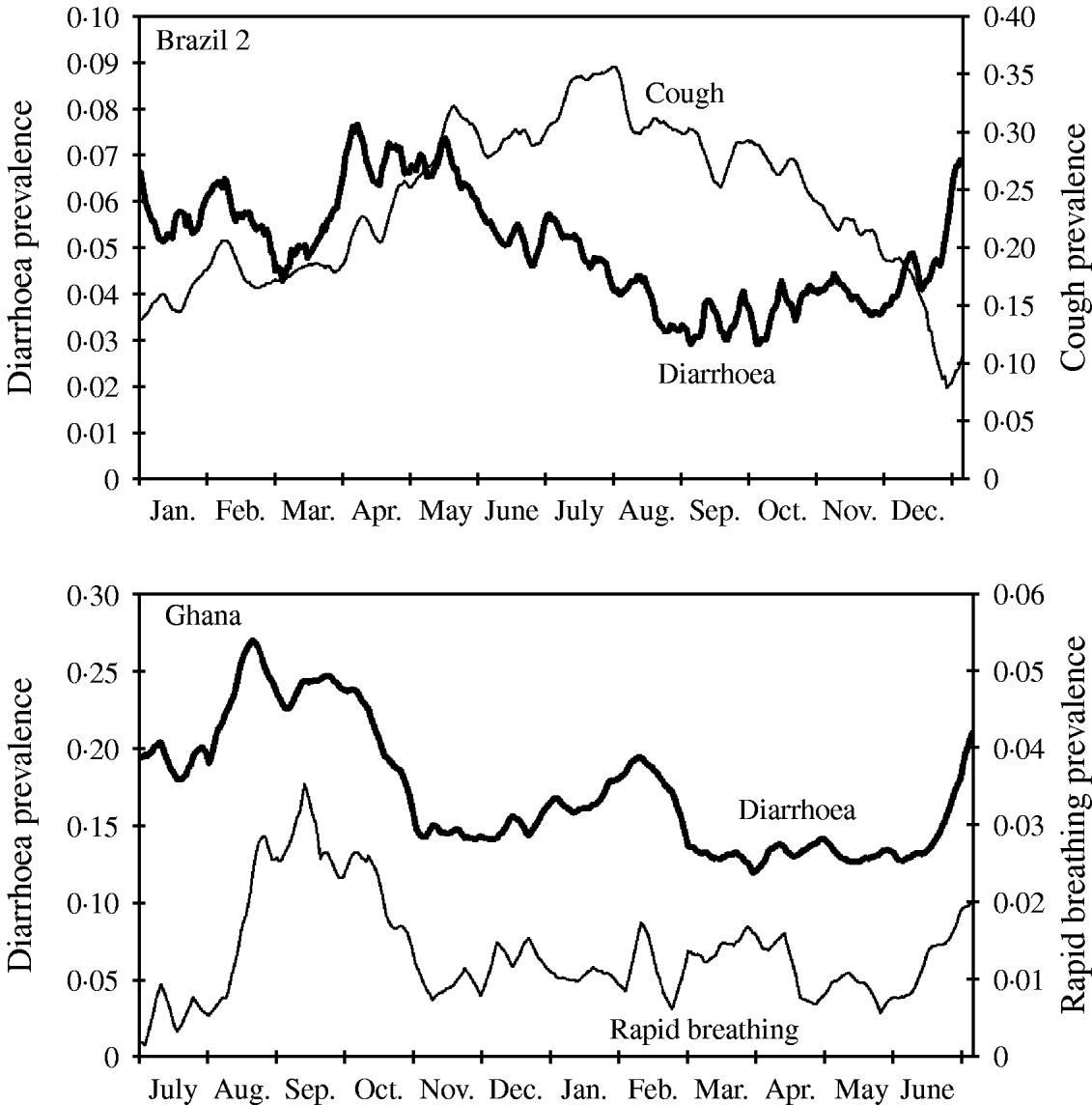
Fig. 5. Seasonal variation of disease shown as weekly moving average of diarrhoea and cough prevalence (Brazil 2), and diarrhoea and rapid breathing (Ghana). Note different time axis in bottom graph (the Ghana study started in summer).
The model can be adapted to generate seasonality with distinct levels (epidemic type) as well as other seasonal patterns, e.g. two peaks of different heights generated by a sinusoidal function to reflect the gradual rise and decline of disease prevalence as observed in Brazil 2.
MODEL APPLICATION
The model may be used for a variety of purposes. It may be particularly helpful to explore different methods of disease surveillance in epidemiological studies or programme evaluation [Reference Schmidt1, Reference Morris3]. For example, many investigators measure the incidence of recurrent infections and conditions by collecting weekly period prevalence data assuming that a new episode starts if there was no disease in the previous week. Models allow the exploration of the extent to which this data collection approach yields imprecise or biased estimates compared to daily data collection. A related modelling approach has been used by Morris et al. [Reference Morris11] and Yoon et al. [Reference Yoon12] to evaluate different surveillance methods for measuring diarrhoea in populations, but instead of simulating the data they only simulated different surveillance schemes directly applied to real data. However, the use of simulated data allows sensitivity analyses to identify key determinants of the simulation results by varying one model parameter at a time while leaving others constant.
The model can also be used to explore the effect of recall error on disease estimates. Recall error can occur in different ways, e.g. by simply forgetting disease occurrence more then a few days ago, or by remembering disease to have occurred closer to the date of a surveillance visit; finally, by field workers rounding disease days to full weeks, which obviously happened in Ghana (Fig. 2).
The model can also provide insights into the epidemiology of diarrhoea and other recurrent diseases by comparing the expected distribution of episodes (or intervals between episodes) under certain assumptions, with the distribution observed in the field [Reference Morris3]. In addition, by making simple assumptions about the dependence of disease risk on a previous episode, one can explore different approaches to estimate the autocorrelation between episodes within individuals. For example, autocorrelation may depend on disease definition (see above) and may also be overestimated unless the analysis is adjusted for confounding factors like the individual number of episodes and seasonality. Unlike real data, autocorrelation can be pre-specified in the model so that one knows what to expect in the analysis.
MODEL LIMITATIONS
Despite introducing additional parameters, the structure of our simulation model is still relatively simple and – as any model – relies on a number of assumptions. For example, the assumed autocorrelation structure is a simplification as the risk of a new episode only depends on the time since the last episode, but not its severity, nor the occurrence of disease prior to this. As with most mathematical models it often pays to start with simple assumptions. In some circumstances it may, however, be necessary to extend the model, e.g. to allow for a more complex autocorrelation pattern, missing data or disease severity. In contrast, some research questions may not require the specification of all parameters described in this paper.
Assuming a gamma distribution for episode incidence and durations does not always result in a good model fit. For example, the gamma distribution underestimated the proportion of individuals with ⩾20 episodes in Brazil 1 (Fig. 1), and also did not fit well the distribution of episode durations observed in DRC (Fig. 2). More complex assumptions would be needed to achieve a better fit in these cases, which may compromise model interpretation. In most cases it may be more appropriate to conduct a sensitivity analysis by simulating a group of outliers to explore whether the conclusions are affected by the lack of fit. Probability distribution functions other than the gamma distribution may also be appropriate to represent skewed data. Since the gamma distribution has been used before in this context and showed a good fit [Reference Schmidt1, Reference Morris3], we used it again for pragmatic reasons.
In conclusion, our simulation model may be primarily useful to improve the methods of measuring recurrent infections and conditions in epidemiological studies, and to explore which statistical approaches are the adequate for data analysis. This paper focuses on diarrhoeal diseases, since many of the parameters like illness duration and autocorrelation of diarrhoeal episodes are of particular public health interest and have therefore been the focus of many studies [Reference Genser9, Reference Baqui14, Reference Victora15]. However, applying the model to other recurrent infections and conditions should be straightforward, as shown by the included examples for other conditions. It is important to note that the use of models does not diminish the need for a sound theoretical basis of a particular research question. Often, appropriate use of statistical theory will allow the prediction of model results. Simulations can then be used to confirm the predictions and provide results applicable to the field.
APPENDIX
Figure A1 is an example of a model structure assuming no seasonality and no overlap between episodes, and a twofold risk of disease during the first 2 weeks after an episode (i.e. two discrete risk levels). The first step in the model generation is the determination of the number of episodes of each simulated individual. This is done (using the method of the inverse cumulative distribution function) [Reference Gentle20] by drawing a uniformly distributed random number between 0 and 1, and applying this number to the inversed cumulative gamma distribution (Fig. A1 a). In this example, the random number results in a value of 5·0, indicating that this individual will have a daily risk of disease of 5·0 episodes per 365 days. Whether this individual will experience an episode on a particular day is decided by drawing another uniformly distributed random number between 0 and 1. If this number is below 5/365, then this day marks the start day of an episode. For every episode, the duration is drawn in a similar manner from the inverse cumulative gamma distribution for episode durations (Fig. A1 b). The allocated duration is then multiplied by the subject-specific error factor to simulate intra-subject correlation, and by a linear function (y=a+bx) to simulate correlation between incidence and duration. The subject-specific error factor is drawn from a normal distribution with mean 1·0. The variance of the normal distribution is incrementally fitted so that the simulated standard deviation of the mean episode durations in individuals is close to that in the observed data. With regard to the linear function, intercept a is the mean duration of episodes in subjects with one episode and slope b the change in episode duration for each additional episode. As there are no episodes lasting for 0 days, the episode durations resulting from this procedure are rounded up to the next whole number. In this case the first episode is allocated a duration of 3 days. The risk of disease is 0 for the duration of the episode, after which the risk rises to 10/365 to simulate the doubled risk after an episode. In this example the individual experiences another episode 3 days after the first episode. The new episode duration (2 days) is again drawn at random from the gamma distribution (Fig. A1 b). During the 14 days after the second episode no further episode occurs. The risk therefore drops to the baseline daily risk of 5/365.
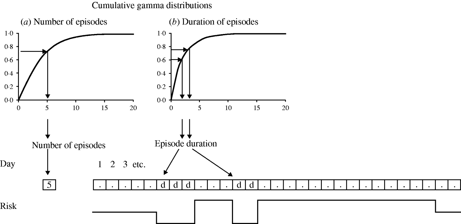
Fig. A1. Model structure.
ACKNOWLEDGEMENTS
The authors are grateful to Mauricio L. Barreto, Stephen P. Luby, Saul Morris, and David Ross for providing datasets for the parameters estimation; and to Thomas Clasen, Sandy Cairncross, Simon Cousens, Clarence Tam, Shakoor Hajat and Lucy Smith for their comments and support. The study was funded by the Wellcome Trust, UK (grant no. WT082569AIA).
DECLARATION OF INTEREST
None.


