


Impact Statement
Supervised deep learning approaches in climate studies, especially in satellite observations, are very limited in application due to the non-conventional nature of the data and the lack of available annotated samples. The present feasibility study on unsupervised domain adaptation aims to increase the compatibility of a deep learning model pre-trained on one satellite to many more with similar physical characteristics. While previous approaches focus on qualitative aspects and classification tasks, the present objective involves a regression task on non-RGB (red, green, and blue) image data. The adaptation results significantly impact the practical perspectives of applying deep learning models to the spatial observation of the earth. In terms of climate studies, this unsupervised transfer learning approach will improve the knowledge of the precipitation evolution over the last 30 years.
1. Introduction
The estimation of precipitation for a given date and location is a very challenging task because rain is very intermittent in time and space. Ground-based observations alone could be very lacking due to the difficulty in obtaining a uniformly calibrated observation with a good spatial resolution over a large region, especially over the oceans (Hou et al., Reference Hou, Kakar, Neeck, Azarbarzin, Kummerow, Kojima, Oki, Nakamura and Iguchi2014). On the other hand, global satellite coverage offers a great advantage in estimating uniform global precipitation. For this exact purpose, the Global Precipitation Measurement (GPM, 2014-present) mission, the successor of the Tropical Rainfall Measuring Mission (TRMM 1997–2015) (Kummerow et al., Reference Kummerow, Barnes, Kozu, Shiue and Simpson1998), has launched a mother satellite called the GPM Core Observatory and a constellation of daughters. Aboard the GPM Core Observatory, a passive microwave radiometer (GPM Microwave Imager or GMI) provides the brightness temperatures, while a dual-frequency precipitation radar (DPR) provides a more direct measurement of the precipitation. The main purpose of the Core Observatory is to serve as the reference for unifying the precipitation estimates from the other satellites in the constellation. The co-located data of brightness temperatures and surface rain rates also open up the opportunity to develop a supervised deep-learning model for rain retrieval. Numerous studies have been done on the subject of rain retrieval, with a list of literature available in Viltard et al. (Reference Viltard, Lepetit, Mallet, Barthès and Martini2020).
Viltard et al. (Reference Viltard, Lepetit, Mallet, Barthès and Martini2020) developed a deep learning model using U-Net for rain retrieval (DRAIN) on the co-located data of the GPM Core Observatory. U-Net is a fully convolutional neural network containing a contraction path, an expansion path, and skip connections (Ronneberger et al., Reference Ronneberger, Fischer and Brox2015). In DRAIN, U-Net is trained to estimate quantiles of rain products with the brightness temperature from the GMI as inputs and the rain rates of the DPR as targets, with further details available in (Viltard et al. (Reference Viltard, Lepetit, Mallet, Barthès and Martini2020)). The next step is to take full advantage of the GPM constellation with this deep learning approach. The GPM constellation, made up of a network of international satellites, can provide up to 80
 $ \% $
of the global coverage in less than 3 hr (Hou et al., Reference Hou, Kakar, Neeck, Azarbarzin, Kummerow, Kojima, Oki, Nakamura and Iguchi2014). Successfully utilizing the whole constellation of GPM will offer a uniform global precipitation map.
$ \% $
of the global coverage in less than 3 hr (Hou et al., Reference Hou, Kakar, Neeck, Azarbarzin, Kummerow, Kojima, Oki, Nakamura and Iguchi2014). Successfully utilizing the whole constellation of GPM will offer a uniform global precipitation map.
GPM official radiometer algorithm is based upon a Bayesian approach in which the GPM core satellite is used to generate an a priori database of observed cloud and precipitation profiles (Passive Microwave Algorithm Team Facility, 2017). One year (September 2014–August 2015) of matched GMI/hydrometeor observations is used to construct the a priori database. The combined product is built with a forward radiative transfer model calculation to compute brightness temperature sets for the different radiometers, that is to say, with different frequency channels and viewing angles. As a description of temperature and water vapor profiles and surface emissivity is needed to perform the simulations, ancillary data coming from Global Climate Models (GCM) reanalysis are associated with each pixel. The variability of the spatial resolution of the different PMRs (Passive Microwave Radiometers) of the constellation is neglected in GPM-V5 (Global Precipitation Measurement Mission Algorithms - version 5). The use of simulated brightness temperatures to develop the retrieval algorithm is an important source of uncertainty, especially in the presence of scattering by hydrometeors. The differences in PMR’s field of view that are not taken into account can also introduce significant errors (Kidd et al., Reference Kidd, Matsui, Chern, Mohr, Kummerow and Randel2016).
As DRAIN is trained on the co-located brightness temperatures and rain rates from the GMI and the DPR, respectively, this model only works for the brightness temperatures of the GPM Core Observatory. This model could not be applied directly to the constellation because, between different satellites, there are differences in viewing angle, frequency band, and spatial resolution. In addition, these other satellites are only equipped with microwave imagers; therefore, there is no co-located data available for a supervised learning approach. To benefit from the frequent revisit time and better coverage of the whole constellation, a method to transfer the knowledge gained from the GPM Core Observatory is required. Transfer learning differs from traditional machine-learning algorithms as it relies on previously trained knowledge. In a traditional machine-learning algorithm, a model is trained on the source domain and is applied to the source domain. Current machine-learning techniques, which have given very good results in the field of computer vision, require a large database to train on and are only valid for this domain. As a result, a new model needs to be trained each time the data are from a different feature space or distribution. On the other hand, in transfer learning, a model is first trained with the source domain. Next, the knowledge is transferred in order to create a model for a new task. This is particularly advantageous in many cases where there is a lack of data for the targeted task but an abundance of data in a similar domain.
The first challenge in transferring the knowledge is, of course, the lack of training data in the target domain. It is possible to co-locate various satellite observations and GPM Core Observatory data. However, due to the highly intermittent nature of rain and the difference in orbit of the satellites, co-located data are very scarce and certainly inefficient for relying on fine-tuning as a method of transfer learning. To use as many satellites data as possible, we have to turn to the transductive transfer learning methods, where the target domain labels are unavailable while the source domain labels are available (Pan and Yang, Reference Pan and Yang2010). With some unsupervised methods, the domain adaptation and regression could be achieved with one model, for example, the Unsupervised Domain Adaptation by Back-propagation (UDA) (Ganin and Lempitsky, Reference Ganin and Lempitsky2015). In UDA, there are three components: the feature extractor, the label predictor, and the domain classifier (Ganin and Lempitsky, Reference Ganin and Lempitsky2015). By integrating the domain classifier within the model, UDA is able to make the two domains as common as possible while providing the predictions at the same time. Though with several modifications tested, this model could not be successfully implemented to this experiment. We have then turned to a domain adaptation method done outside of the rain retrieval model. To perform this domain adaptation task, the CycleGAN was used.
The end goal is to adapt any satellite scans in the GPM Constellation (target domain) to that of the GPM Core Observatory (source domain) in order to be able to use the U-Net for rain retrieval previously trained on the source domain. In the feasibility study presented here, the GMI 89 GHz channels in horizontal and vertical polarization (hereafter 89H and 89 V) are the two domains to be adapted using CycleGAN. In the following text, Section 2 describes the domain adaptation method. Next, Section 3 provides details about the data used for training and testing. Section 4 shows the evaluation of the method in terms of the similarity between the original and adapted domain as well as its performance in rain retrieval. Finally, in Section 5, the next steps and possible improvements will be discussed.
2. Method
The method used in this feasibility study consists of applying an unsupervised domain adaptation on satellite images using a Generative Adversarial Nets (GAN; Goodfellow et al., Reference Goodfellow, Pouget-Abadie, Mirza, Xu, Warde-Farley, Ozair, Courville and Bengio2014) based approach called CycleGAN (Zhu et al., Reference Zhu, Park, Isola and Efros2017a). Then, the newly transformed images are tested on a rain retrieval model that was previously trained with original images.
2.1. CycleGAN
CycleGAN is an image transformation technique that does not require paired images (Zhu et al., Reference Zhu, Park, Isola and Efros2017a). It consists of two GANs working together, each containing a generator and a discriminator (Figure 1). The first generator
 $ G $
takes an image from the source domain
$ G $
takes an image from the source domain
 $ X $
and transforms it into the target domain
$ X $
and transforms it into the target domain
 $ Y $
. The second generator
$ Y $
. The second generator
 $ F $
works the other way around, by transforming an image in
$ F $
works the other way around, by transforming an image in
 $ Y $
into
$ Y $
into
 $ X $
. The discriminators
$ X $
. The discriminators
 $ {D}_X $
and
$ {D}_X $
and
 $ {D}_Y $
try to correctly label if a sample is from its respective domain.
$ {D}_Y $
try to correctly label if a sample is from its respective domain.

Figure 1. (a) The architecture of CycleGAN. (b) and (c) The illustration of cycle-consistency loss (Zhu et al., Reference Zhu, Park, Isola and Efros2017a).
The weights of the two generators are updated by their combined loss. Each generator has three terms of loss: cycle-consistency loss, identity loss, and adversarial loss. Cycle consistency is based on the idea that a complete image translation cycle (from
 $ X $
to
$ X $
to
 $ Y $
and back to
$ Y $
and back to
 $ X $
) as shown in Figure 1a, should be able to bring back a close enough image to the original (Zhu et al., Reference Zhu, Park, Isola and Efros2017a). The identity loss is included since it has previously shown the ability to preserve color when transforming between photos and painting (Zhu et al., Reference Zhu, Park, Isola and Efros2017a). It is the difference between an image and the transformation to its own domain, for example,
$ X $
) as shown in Figure 1a, should be able to bring back a close enough image to the original (Zhu et al., Reference Zhu, Park, Isola and Efros2017a). The identity loss is included since it has previously shown the ability to preserve color when transforming between photos and painting (Zhu et al., Reference Zhu, Park, Isola and Efros2017a). It is the difference between an image and the transformation to its own domain, for example,
 $ \parallel F(x)-x{\parallel}_1 $
. In the presented experiment, without identity loss, the generator is able to reconstruct the form of the structure but unable to reproduce the value of the brightness temperature. The discriminator loss, on the other hand, is calculated upon its ability to distinguish the real images and the fake images generated by the generators. The complete objective function can be found in Zhu et al. (Reference Zhu, Park, Isola and Efros2017a).
$ \parallel F(x)-x{\parallel}_1 $
. In the presented experiment, without identity loss, the generator is able to reconstruct the form of the structure but unable to reproduce the value of the brightness temperature. The discriminator loss, on the other hand, is calculated upon its ability to distinguish the real images and the fake images generated by the generators. The complete objective function can be found in Zhu et al. (Reference Zhu, Park, Isola and Efros2017a).
Zhu et al. (Reference Zhu, Park, Isola and Efros2017a) concluded that the CycleGAN worked best for color and texture changes, for example, transforming between different painting styles. However, it is less successful when geometric transformation is involved, for example, cat-to-dog transfiguration. Furthermore, de Bézenac et al. (Reference de Bézenac, Ayed and Gallinari2019) emphasized CycleGAN’s capacity to only perform well for distributions that are close to one another. In the experiment here, this is not really a problem because the rain cells have similar geometries whatever the selected channel. Zhu et al. (Reference Zhu, Park, Isola and Efros2017a) also highlighted the impossibility of achieving as good performance as in the case of paired data approach and the failure when the characteristic distribution of the training data is not representative enough of the test data.
2.2. Training details
Several architectures of the generator proposed by Zhu et al. (Reference Zhu, Park, Isola and Efros2017a) were tested. With previous success shown by Viltard et al. (Reference Viltard, Lepetit, Mallet, Barthès and Martini2020), U-Net is a very good candidate for working with satellite images, particularly the brightness temperatures. Using U-Net as generator, the generated images are able to better imitate the structure native to the targeted domain. The second challenge is the imbalance in the training loss between the two domains. In the first few attempts, with the learning rate schedulers for both generators evolving the same way as the training progresses, the losses remain very imbalanced. Hence, different learning rates are set for each generator, with higher learning rates for the generator that seems to struggle more. This results in similar losses for both domains, which may be due to the fact that the two generators work together to establish the cycle-consistency loss. It should also be noted that the batch size has an important impact. In this toy experiment, the batch of sizes 1, 4, 8, and 16 were tested. After several initializations of the network, eight images per batch gave the best results in terms of structure within the satellite observation. Smaller or bigger batch size seems to degrade the results. The batch size effect is an empirical remark made equally on the official GitHub depository of CycleGAN (Zhu et al., Reference Zhu, Park and Tongzhou2017b). Therefore, it should warrant careful testing for future application.
3. Toy Experiment Data
The GMI is a multi-channel conically scanning radiometer with a swath of 904 km and channels ranging from 10 GHz to 183 GHz. These channels are measured in both Horizontal (H) and Vertical (V) polarization. In this toy experiment, only the 89-GHz channel is used. This channel has a resolution of 4.4 km by 7.3 km. We aim to transform between the horizontal and vertical polarization of the GMI 89 GHz channel using CycleGAN. In this case,
 $ X $
in Figure 1 represents 89 V while
$ X $
in Figure 1 represents 89 V while
 $ Y $
represents 89H. This choice of toy data set will later allow comparisons of the adapted image and the targeted satellite scan. The training and validation data sets for each domain do not contain overlapping events to properly test the unpaired image domain adaptation method. The difference between 89H and V is mostly due to the surface emissivity difference between the two channels. The V surface emissivity is almost always higher than the H surface emissivity leading to a generally higher V brightness temperature. However, polarization due to scattering by ice might occur in (rare) cases of oriented particles leading to an H brightness temperature higher than V. This is true for both land and ocean situations.
$ Y $
represents 89H. This choice of toy data set will later allow comparisons of the adapted image and the targeted satellite scan. The training and validation data sets for each domain do not contain overlapping events to properly test the unpaired image domain adaptation method. The difference between 89H and V is mostly due to the surface emissivity difference between the two channels. The V surface emissivity is almost always higher than the H surface emissivity leading to a generally higher V brightness temperature. However, polarization due to scattering by ice might occur in (rare) cases of oriented particles leading to an H brightness temperature higher than V. This is true for both land and ocean situations.
The training data set consists of 24,000 images for each domain, making 48,000 images in total of different observations taken between 2015 and 2017. The validation set is made up of 4,000 images for each domain taken from the same period. These images contain
 $ 221\times 256 $
pixels and are chosen with the conditions that they either have at least 100 pixels with more than 10 mm/hr rain or at least 10 pixels with more than 100 mm/hr rain rates. The selection process is essential to obtain enough images with a precipitation event. Next, the training and validation sets undergo the pre-processing step: data normalization, random crop (to
$ 221\times 256 $
pixels and are chosen with the conditions that they either have at least 100 pixels with more than 10 mm/hr rain or at least 10 pixels with more than 100 mm/hr rain rates. The selection process is essential to obtain enough images with a precipitation event. Next, the training and validation sets undergo the pre-processing step: data normalization, random crop (to
 $ 128\times 128 $
pixels) and random rotation. The random crop (cropping randomly within the image) and random rotation (choosing an angle at random to rotate the image) are added as a data augmentation method and to increase the difficulty of the task for the CycleGAN model. An example of training data is given in Figure 2. Note that, though the example given here is of the same event, neither train nor validation images of each domain correspond to each other.
$ 128\times 128 $
pixels) and random rotation. The random crop (cropping randomly within the image) and random rotation (choosing an angle at random to rotate the image) are added as a data augmentation method and to increase the difficulty of the task for the CycleGAN model. An example of training data is given in Figure 2. Note that, though the example given here is of the same event, neither train nor validation images of each domain correspond to each other.

Figure 2. Vertical (89 V) and horizontal (89H) polarization of the 89-GHz channel brightness temperature in Kelvin from the GMI. The image is of 128 by 128 pixels representing roughly (1,024 km by 1,024 km).
4. Results
Figure 3 shows the training and validation losses. As discussed previously, different learning rate schedules for each domain allow the losses of both domains to evolve in the same way and without a gap between them. According to experiments, this could not be achieved if the learning rates for all networks involved had the same learning rate schedules. To evaluate the performance of CycleGAN on domain adaptation between 89 V and 89 V, its ability to reconstruct complex rain structures, as well as its accuracy in terms of brightness temperatures, are discussed.

Figure 3. Training and validation losses for different components of the CycleGAN. The training loss (first plot) plot shows the generator and discriminator loss throughout training. Then, generator loss plot (second plot) and discriminator loss plot (third plot) show the details of each component. Finally, validation loss plot (fourth plot) shows the cycle consistency and identity loss of each domain on validation dataset.
4.1. Results on adapted satellite images
Figure 4 shows the original satellite scans and the adapted images (89 V adapted from 89H and 89H adapted from 89 V) on a case study. CycleGAN can reproduce very well all the precipitation structures in the original images. However, in terms of values, there are differences in brightness temperature between the original and the adapted images that could not be picked up on qualitatively. Hence, after confirming the re-created structure of brightness temperature for a complex precipitation event, the next step is to investigate the accuracy. With the test data consisting of 2 months of observation, including December 2018 and May 2020, Figure 5 shows the comparison between the original normalized data and the adapted results. The original and adapted histograms are almost superimposed though with some inaccuracy. Calculating the Kullback–Leiber divergence (Bishop et al., Reference Bishop1995) also confirms that there is more similarity between the original and adapted domain than without the transformation.

Figure 4. Original, adapted, and their difference of the 89-GHz channel observation from GMI on the 29th May 2017 with latitude 5–15
 $ {}^{\circ } $
N and longitude 96–105
$ {}^{\circ } $
N and longitude 96–105
 $ {}^{\circ } $
E (over parts of Thailand and Cambodia).
$ {}^{\circ } $
E (over parts of Thailand and Cambodia).

Figure 5. Comparison of the histogram of original 89 V data and the adapted 89 V data (left) and original 89H data and the adapted 89H (right).
4.2. Results on rain retrieval
Relying on the previous work by Viltard et al. (Reference Viltard, Lepetit, Mallet, Barthès and Martini2020), a U-Net model is used to train a rain retrieval model with the GMI 89 GHz channel as input. The U-Net model takes two layers as input; the first is the 89 V and the second is the 89H. The target data is the spatially and temporally co-located data from the DPR of the GPM Core Observatory. The DPR surface rain product is the result from the merging of Ka- (13.4 GHz) and Ku-band (35.5 GHz) radars. It has a horizontal resolution of 5 km and a swath of 245 km. Further information about the treatment of this data is available in Viltard et al. (Reference Viltard, Lepetit, Mallet, Barthès and Martini2020).
The rain retrieval is evaluated on three criteria, its ability to distinguish rain and no-rain cases (Tables 1 and 2), the mean absolute error when compared to the DPR rain rates, and its ability to reconstruct the rain structure. Three cases are compared. Case 1 is the best-case scenario, where the rain retrieval model is tested on [89 V, 89H] input data, the correct order on which it was trained. Case 2, on the other hand, is the worst-case scenario, which is using a model trained on [89 V, 89H] inputs and tested on [89H, 89 V] inputs. In the last one, Case 3, the rain retrieval model is tested on the adapted brightness temperature, that is to say, the pair [89 V (adapted from 89 H), 89 H (adapted from 89 V)]. The objective is to situate ideally as close to Case 1 as possible. Figure 6 shows the rain retrieval in the same case study as in the above subsection. Compared to the ideal case (Case 1), the retrieved rain intensity with the adapted data as inputs (Case 3) is much weaker. In other words, Case 3 has approximately the same structure but is very weak in terms of intensity. Case 2, on the other hand, could not reproduce precipitation at all. Next, the classification score in Table 1 shows the ability to distinguish between rain and no rain cases. No-rain cases refer to the prediction below 0.1 mm/hr. With domain adaptation, clear improvement was observed across all scores. We could also observe a small improvement in terms of the mean absolute error score in Table 2.
Table 1. Classification score for rain vs no-rain cases using the two-month test data.

Table 2. Mean absolute errors using the two-month test data.
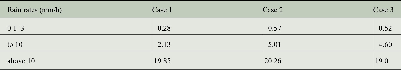

Figure 6. (Same observation as Figure 4) Comparison of retrieved surface rain rates in mm/h in Case 1 (left), Case 2 (middle), and Case 3 (right).
5. Conclusions and Perspectives
Although this domain adaptation method performs very well in terms of qualitative assessment, there is still room for improvement in its application in rain retrieval. Based on the results presented in Section 4, the pre-trained U-Net model is very sensitive to both the structure and, in turn, the gradient, as well as the value of the brightness temperature itself. Nevertheless, the results from this toy experiment present a promising proof of concept. The next step would be to study the real application with the GPM core observatory as the source domain and one of the satellites in the constellation, for example, SSMI/S, as the target domain. This feasibility study also highlights the importance of quantitative assessment in image domain adaptation for a regression task. In order to give a better estimation, a more elegant approach consists of constraining the CycleGAN training process with the loss from the rain retrieval model. Prior works related to this approach include the Conditional Generative Adversarial Nets (Conditional GAN) (Mirza and Osindero, Reference Mirza and Osindero2014) and one of its many variations, Red-GAN (Qasim et al., Reference Qasim, Ezhov, Shit, Schoppe, Paetzold, Sekuboyina, Kofler, Lipkova, Li and Menze2020). In Conditional GAN, additional information, for example, class label, is added to the training of the GANs. Red-GAN is built upon the concept of Conditional GAN with a third-player integrated into the two-player Conditional GAN (generator and discriminator) in order to better favor the final objective. In future applications on rain retrieval, the U-Net could become an extension of the CycleGAN model. The error in rain rate could then be integrated into the training loss in order to update the generators and discriminator’s weights. As a consequence, the domain adaptation process is constrained to best work on the rain retrieval application.
Author Contributions
Conceptualization: V.S., N.V., L.B., A.M., C.M.; Data curation: N.V.; Data visualization: V.S., N.V.; Methodology: V.S., L.B., C.M.; Writing—original draft: V.S. All authors approved the final submitted draft.
Competing Interests
The authors declare no competing interests exist.
Data Availability Statement
The 1C-R.GPM.GMI.XCAL2016-C, 2A.GPM.DPR.V8 and 2A.GPM.GMI.GPROF2017v1 data sets were provided by the NASA/Goddard Space Flight Center and PPS, which develop and compute these data sets as a contribution to GPM, and archived at the NASA GES DISC.
Ethics Statement
The research meets all ethical guidelines, including adherence to the legal requirements of the study country.
Funding Statement
This research was supported by the EUR IPSL and CNES-TOSCA.
Provenance
This article is part of the Climate Informatics 2022 proceedings and was accepted in Environmental Data Science on the basis of the Climate Informatics peer review process.


 Open access