


Impact Statement
PM2.5 pollution poses significant health risks and is responsible for millions of deaths per year. Our work forecasts the PM2.5 concentration at sparse locations and estimates the fire-specific PM2.5 contribution to assess their impact on air quality. Furthermore, prescribed fires, while preventing wildfires, also generate PM2.5, raising concerns about the air quality trade-offs. To the best of our knowledge, our work is the first to apply machine learning to predict the PM2.5 concentration from simulated prescribed fires. We use our forecasting model to conduct novel experiments that can help the fire service better understand and minimize the pollution exposure from prescribed fires.
1. Introduction
Across many parts of the western United States (WUS), wildfire size, severity, and fire season length have increased due to climate change (Williams et al., Reference Williams, Abatzoglou and Gershunov2019). Wildfires across the WUS have led to the largest daily mean PM2.5 (particulate matter <2.5 microns) concentrations observed by ground-based sensors in recent years (Burke et al., Reference Burke, Driscoll and Heft-Neal2021) and exposure to PM2.5 is responsible for 4.2 million premature deaths worldwide per year (World Health Organization, 2022). Within California, additional PM2.5 emissions from extreme wildfires over the past 8 years have reversed nearly two decades of decline in ambient PM
 $ {}_{2.5} $
concentrations (Burke et al., Reference Burke, Childs and de la Cuesta2023).
$ {}_{2.5} $
concentrations (Burke et al., Reference Burke, Childs and de la Cuesta2023).
Due to the numerous severe health consequences from PM2.5 pollution exposure, performing accurate and temporally fine-grained PM
 $ {}_{2.5} $
predictions has become increasingly significant. A recent study by Aguilera et al. (Reference Aguilera, Corringham and Gershunov2021) found the PM2.5 emitted from wildfires to be more toxic than the PM2.5 emitted from ambient sources. Accurate PM2.5 predictions are also important in the context of prescribed fires, or controlled burns, which have been widely accepted as an effective land management tool and could have the potential to reduce the resulting smoke from future wildfires (Kelp et al., Reference Kelp, Carroll and Liu2023). Since air quality is a major public concern surrounding prescribed fires (McCaffrey, Reference McCaffrey and Dickinson2006), land managers conducting these burns require access to robust, near real-time predictions of downwind air pollution, to determine suitable locations and burn windows.
$ {}_{2.5} $
predictions has become increasingly significant. A recent study by Aguilera et al. (Reference Aguilera, Corringham and Gershunov2021) found the PM2.5 emitted from wildfires to be more toxic than the PM2.5 emitted from ambient sources. Accurate PM2.5 predictions are also important in the context of prescribed fires, or controlled burns, which have been widely accepted as an effective land management tool and could have the potential to reduce the resulting smoke from future wildfires (Kelp et al., Reference Kelp, Carroll and Liu2023). Since air quality is a major public concern surrounding prescribed fires (McCaffrey, Reference McCaffrey and Dickinson2006), land managers conducting these burns require access to robust, near real-time predictions of downwind air pollution, to determine suitable locations and burn windows.
However, most data-driven PM2.5 forecasting algorithms do not distinguish between ambient PM2.5 concentration and the additional concentration due to fire emissions. Previous work studying the effect of prescribed fires on pollution used chemical transport models (CTMs) like the Community Multiscale Air Quality (CMAQ) and Goddard Earth Observing System Atmospheric Chemistry (GEOS-Chem) models to calculate the PM2.5 impact of prescribed fires at different locations (Kelp et al., Reference Kelp, Carroll and Liu2023). Jin et al. (Reference Jin, Permar and Selimovic2023) and Schollaert et al. (Reference Schollaert, Marlier and Marshall2024) used CTMs to study prescribed fires in the Western United States. Although CTMs can model the complex chemical processes in PM2.5 transport, their computational expense is a drawback in generating accurate predictions as well as exploring a large parameter space for simulating prescribed burns (Askariyeh et al., Reference Askariyeh, Khreis, Vallamsundar and Khreis2020; Byun and Schere, Reference Byun and Schere2006; Zaini et al., Reference Zaini, Ean and Ahmed2022; Rybarczyk and Zalakeviciute, Reference Rybarczyk and Zalakeviciute2018).
Recent analyses have combined satellite-based observations with meteorological data to derive daily wildfire-specific PM2.5 for all ZIP codes in California (Aguilera et al., Reference Aguilera, Luo and Basu2023) and in 10 km grid cells across the contiguous United States (Childs et al., Reference Childs, Li and Wen2022). Both these studies relied on smoke plume boundaries identified by expert input to identify smoke exposure per day and grid cell, and used the PM2.5 measurements on non-smoke days to estimate the PM2.5 contribution from background sources. Specifically, Childs et al. (2022) (Childs et al., Reference Childs, Li and Wen2022) defined wildfire-specific PM2.5 as anomalies relative to monthly mean PM2.5 concentration in each grid cell and adopted gradient-boosted trees to predict the anomalous PM2.5 as a function of fire-related predictors. On the other hand, Aguilera et al. (Reference Aguilera, Luo and Basu2023) trained an ensemble of machine learning models to first estimate the total PM2.5 concentration for each ZIP code, then obtained the wildfire-specific PM2.5 by subtracting the background PM2.5 imputed from model predictions of PM2.5 for non-smoke days. Meanwhile, Qiu et al. (Reference Qiu, Kelp and Heft-Neal2024) found that CTMs overestimated the PM2.5 concentrations for extreme smoke events in 2020 while the wildfire-specific PM2.5 predictions from the Childs et al. (Reference Childs, Li and Wen2022) machine learning model were in much better agreement with surface PM2.5 measurements.
Our research builds upon the GNN-GRU machine learning model named PM2.5-GNN from Wang et al. (Reference Wang, Li and Zhang2020), which was used to forecast non-wildfire-influenced PM
 $ {}_{2.5} $
pollution in China. In contrast, our work focuses on predicting fire-influenced PM2.5 at different sensor locations across California. The spatio-temporal modeling capabilities of the PM2.5-GNN coupled with domain knowledge make the model especially valuable for PM2.5 prediction with spatially sparse monitor observations, enabling the PM2.5-GNN to outperform baseline machine learning architectures such as random forest (RF), long short-term memory (LSTM), and multilayer perceptron (MLP) models. Our PM2.5-GNN model predicts the PM2.5 pollution at an hourly resolution in California and considers two applications: (1) quantifying fire-specific PM2.5 concentration and (2) forecasting the pollution levels emitted from simulated prescribed fire events. Specifically, we incorporate satellite-derived data on fire intensity within the PM2.5-GNN model to forecast PM2.5 concentration from ambient sources, observed fires, and simulated controlled burns.
$ {}_{2.5} $
pollution in China. In contrast, our work focuses on predicting fire-influenced PM2.5 at different sensor locations across California. The spatio-temporal modeling capabilities of the PM2.5-GNN coupled with domain knowledge make the model especially valuable for PM2.5 prediction with spatially sparse monitor observations, enabling the PM2.5-GNN to outperform baseline machine learning architectures such as random forest (RF), long short-term memory (LSTM), and multilayer perceptron (MLP) models. Our PM2.5-GNN model predicts the PM2.5 pollution at an hourly resolution in California and considers two applications: (1) quantifying fire-specific PM2.5 concentration and (2) forecasting the pollution levels emitted from simulated prescribed fire events. Specifically, we incorporate satellite-derived data on fire intensity within the PM2.5-GNN model to forecast PM2.5 concentration from ambient sources, observed fires, and simulated controlled burns.
Our GNN-based forecasting framework can help policymakers better isolate the PM2.5 concentration emitted from wildfires. While studies like Childs et al. (Reference Childs, Li and Wen2022) and Qiu et al. (Reference Qiu, Kelp and Heft-Neal2024) rely on analyst-derived information, such as plume boundaries, to identify non-smoke days for calculating median PM2.5 values per grid cell and month, our method operates without the need for expert input. This makes it suitable for rapid deployment as a fast and efficient emergency management tool. Additionally, our forecasts can aid forest managers in minimizing the PM2.5 exposure of vulnerable populations during controlled burns and facilitate community discussions of potential locations and burn windows for prescribed fires. Thus, while several studies have used machine learning to forecast air quality (Wang et al., Reference Wang, Li and Zhang2020; Li et al., Reference Li, Wang and Franklin2023) as well as to estimate wildfire-specific PM2.5 (Aguilera et al., Reference Aguilera, Luo and Basu2023; Childs et al., Reference Childs, Li and Wen2022), this is the first paper, to the best of our knowledge, that utilizes machine learning to predict the PM2.5 concentration at sensor locations from simulated prescribed fires. Although we focus on PM2.5 predictions at sparse sensor locations, our method could be extended to predictions over both ZIP codes and a regular grid.
The remainder of the paper is organized as follows: the fire and meteorological data used in our analyses are detailed in Section 2. In Section 3.1, we describe the PM2.5-GNN model and validate its PM2.5 predictions with baseline machine learning models. The model setup for estimating wildfire-specific PM2.5 is outlined in Section 3.2. Sections 4.1 and 4.2 present, respectively, idealized experiments using a framework based on the PM2.5-GNN model to determine the optimal time to implement prescribed fires and to quantify the reduction in air quality impact due to mitigation of larger wildfires. We discuss the paper’s conclusions and potential directions for future work in Section 5.
2. Dataset
Our dataset consists of PM2.5, meteorological, and fire data at an hourly resolution over 5 years (2017–21). The PM2.5 concentration data, at a total of 112 sparse air quality sensor locations in California shown in Figure 9, is collected from both the California Air Resources Board (CARB) as well as the Environmental Protection Agency (EPA) (California Air Resources Board, n.d.; US Environmental Protection Agency, n.d.). The MissForrest algorithm (Stekhoven and Bühlmann, Reference Stekhoven and Bühlmann2011) was used to impute the missing PM2.5 observations from offline sensors. The data for the seven meteorological predictors, which include u and v horizontal components of wind, total precipitation, and air temperature, are retrieved from the ERA5 Reanalysis database (Hersbach et al., Reference Hersbach, Bell and Berrisford2020). We provide the full list of predictors in Table 1. Though the meteorological predictors may capture the diurnal PM2.5 cycles and seasonal patterns, the Julian date and hour of the day are also included as predictors to provide the model with additional context.
Table 1. Dataset predictors and PM2.5-GNN node features

The fire radiative power (FRP) provides information about the fire intensity. The FRP at each fire location is taken from the Visible Infrared Imaging Radiometer Suite (VIIRS) (Schroeder and Giglio, Reference Schroeder and Giglio2017) instrument on board the Suomi satellites. To assess the impact of nearby fires at the location of a PM2.5 monitor, we aggregate the FRP values of all active fires within radii of 25, 50, 100, and 500 km. To emphasize the fires that would likely have a more substantial downwind effect on PM2.5 concentration, we use inverse distance weighting (IDW) and wind-based weighting in the FRP aggregation. For each PM2.5 monitor location, aggregations are performed on radii of 25, 50, 100, and 500 km to derive the wind and inverse-distance weighted (WIDW) FRP using the process described in Figure 1 and
 $$ {F}_{\mathrm{WIDW}}=\sum \limits_{i=1}^n\frac{F_i\left|{V}_i\right|\cos \left(\left|{\alpha}_i\right|\right)}{4\pi {R_i}^2} $$
where
 $ n $
is the number of fire locations within a certain radius of the PM2.5 monitor site,
$ n $
is the number of fire locations within a certain radius of the PM2.5 monitor site,
 $ F $
is the FRP value at the fire location,
$ F $
is the FRP value at the fire location,
 $ \mid V\mid $
is the magnitude of the wind speed at the fire location,
$ \mid V\mid $
is the magnitude of the wind speed at the fire location,
 $ \alpha $
is the relative angle between the wind direction and the direction from the fire to the PM2.5 monitor, and
$ \alpha $
is the relative angle between the wind direction and the direction from the fire to the PM2.5 monitor, and
 $ R $
is the distance between the fire site and PM2.5 monitor. The number of fires within 500 km of a PM2.5 site is also included in the dataset. The prescribed fire latitude, longitude, and duration data retrieved from the California Department of Forestry and Fire Protection (Cal Fire) (Cal Fire, Reference Firen.d.) is not represented as a variable in the training dataset but instead used in Experiments 1 and 2 when simulating prescribed fires.
$ R $
is the distance between the fire site and PM2.5 monitor. The number of fires within 500 km of a PM2.5 site is also included in the dataset. The prescribed fire latitude, longitude, and duration data retrieved from the California Department of Forestry and Fire Protection (Cal Fire) (Cal Fire, Reference Firen.d.) is not represented as a variable in the training dataset but instead used in Experiments 1 and 2 when simulating prescribed fires.

Figure 1. FRP aggregated around a given radius for each PM
 $ {}_{2.5} $
monitor location using wind and distance information.
$ {}_{2.5} $
monitor location using wind and distance information.
3. PM2.5 forecasts
3.1. PM2.5-GNN model
3.1.1. Methods
We trained the spatio-temporal PM2.5-GNN model from Wang et al. (Reference Wang, Li and Zhang2020), to predict PM2.5 concentration at an hourly temporal resolution utilizing spatially sparse observations, as illustrated in Figure 2. In Figure 2,
 $ {v}_i $
,
$ {v}_i $
,
 $ {v}_j $
,
$ {v}_j $
,
 $ {F}^{v_i} $
, and
$ {F}^{v_i} $
, and
 $ {F}^{e_{ij}} $
, respectively, refer to nodes
$ {F}^{e_{ij}} $
, respectively, refer to nodes
 $ i $
and
$ i $
and
 $ j $
, the feature vector for node
$ j $
, the feature vector for node
 $ i $
, and the feature vector for edge
$ i $
, and the feature vector for edge
 $ {e}_{ij} $
. The PM2.5-GNN model consists of two components: a graph neural network (GNN) to learn the PM2.5 spatial propagation between monitor sites and a Gated Recurrent Unit (GRU) to capture the temporal diffusion process. The GNN model has a directed graph, where nodes represent the locations of PM2.5 monitors and edges model the PM2.5 movement and interactions between monitors, making it well-suited to leverage non-homogeneous data. Thus, the node features include all the meteorological and fire-related predictors, as shown in Table 1. The edge attributes consist of the wind speed of the source node, the distance between the source and sink, the wind direction of the source node, the direction from source to sink, and an advection coefficient that quantifies the degree of wind impact on the sink node by the source node. In the graph model of PM2.5 transport, the source node represents the site where the PM2.5 was initially detected at a specific time point and the sink node represents a location downwind of the initial site. Domain knowledge is incorporated in the graph representation through the choice of node and edge attributes, as well as through the choice of the graph connectivity. For instance, the graph explicitly includes wind direction information and considers geographical elevation differences. The GNN only models the transport of PM2.5 between two sites if they are within 300 km of one another and if the elevation difference between the sites is < 1200 m. The altitude threshold was established on the assumption that differences in elevation >1200 m between sites would hinder PM2.5 transport.
$ {e}_{ij} $
. The PM2.5-GNN model consists of two components: a graph neural network (GNN) to learn the PM2.5 spatial propagation between monitor sites and a Gated Recurrent Unit (GRU) to capture the temporal diffusion process. The GNN model has a directed graph, where nodes represent the locations of PM2.5 monitors and edges model the PM2.5 movement and interactions between monitors, making it well-suited to leverage non-homogeneous data. Thus, the node features include all the meteorological and fire-related predictors, as shown in Table 1. The edge attributes consist of the wind speed of the source node, the distance between the source and sink, the wind direction of the source node, the direction from source to sink, and an advection coefficient that quantifies the degree of wind impact on the sink node by the source node. In the graph model of PM2.5 transport, the source node represents the site where the PM2.5 was initially detected at a specific time point and the sink node represents a location downwind of the initial site. Domain knowledge is incorporated in the graph representation through the choice of node and edge attributes, as well as through the choice of the graph connectivity. For instance, the graph explicitly includes wind direction information and considers geographical elevation differences. The GNN only models the transport of PM2.5 between two sites if they are within 300 km of one another and if the elevation difference between the sites is < 1200 m. The altitude threshold was established on the assumption that differences in elevation >1200 m between sites would hinder PM2.5 transport.
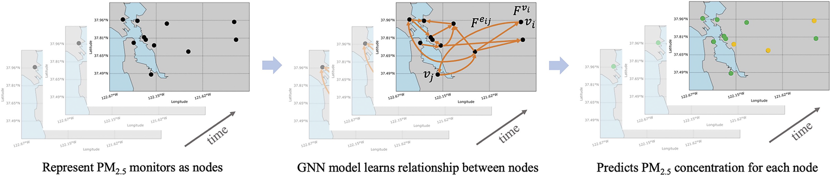
Figure 2. Graph neural network (GNN) used in our PM2.5 forecasting model considers PM2.5 monitors as nodes in the graph and produces node-level predictions.
As shown in Table 2, for the PM2.5-GNN model, 2 years are used for training and 1 year each for validation and testing. In total, we use ~1.96 million samples for training and 0.98 million samples each for validation and testing. The year 2019 is excluded during training, validation, and testing because the 2019 fire season was an outlier and was less damaging than the other years. Validating and testing the model on data from the years 2020 and 2021, respectively, would help us gain a better understanding of the model’s performance during intense fires, as both 2020 and 2021 had severe wildfire seasons. Our model produces PM2.5 forecasts for a prediction window of 48 hours into the future based on a model initialized with PM2.5 observations in a historical window of 240 hours.
Table 2. Training/validation/testing split

3.1.2. Results
For the evaluation of the PM2.5-GNN’s performance, we analyzed heat maps of the observed versus predicted PM2.5 concentrations for various future time points (1-hour, 12-hour, and 48-hour forecasts), as shown in Figure 3. The color scale represents the density of points within a bin, with bin boundaries selected on a logarithmic scale. Perfect predictions would align along the 1:1 line, while deviations from this line in specific directions indicate prediction errors. Similar heat map graphs of observed versus predicted PM2.5 were presented in Considine et al. (2023) (Considine et al., Reference Considine, Hao and de Souza2023). For our 1-hour forecasts, there is a high density of points along the identity (y = x) line, indicating the model’s ability to predict PM2.5 levels close to the observed values. However, the heat maps also reveal that the model begins to underpredict more severely for observed PM2.5 concentrations exceeding
 $ \approx $
200 μg/m3. The PM2.5-GNN model’s
$ \approx $
200 μg/m3. The PM2.5-GNN model’s
 $ {R}^2 $
value is lower than those reported in Considine et al. (Reference Considine, Hao and de Souza2023) and Qiu et al. (Reference Qiu, Kelp and Heft-Neal2024), which both studied PM2.5 predictions using machine learning, because our predictions are at an hourly resolution, whereas theirs are at a daily resolution. As the PM2.5-GNN model predicts further into the future, the
$ {R}^2 $
value is lower than those reported in Considine et al. (Reference Considine, Hao and de Souza2023) and Qiu et al. (Reference Qiu, Kelp and Heft-Neal2024), which both studied PM2.5 predictions using machine learning, because our predictions are at an hourly resolution, whereas theirs are at a daily resolution. As the PM2.5-GNN model predicts further into the future, the
 $ {R}^2 $
value and the density of the points along the identity line for elevated concentrations decrease. The decreasing accuracy of predictions for time steps further into the future is a challenge inherent to prediction tasks.
$ {R}^2 $
value and the density of the points along the identity line for elevated concentrations decrease. The decreasing accuracy of predictions for time steps further into the future is a challenge inherent to prediction tasks.

Figure 3. Heat maps illustrating the observed PM2.5 concentrations versus the PM2.5-GNN model predictions for 1-, 12-, and 48-hour forecasts, with log-transformed axes and color scale. Also indicated is the identity line (dotted black) and
 $ {R}^2 $
values of the best-fit linear model.
$ {R}^2 $
values of the best-fit linear model.
To further evaluate the PM2.5-GNN model, its performance was compared to three baseline models, the random forest (RF), long short-term memory (LSTM), and multilayer perceptron (MLP) models. The PM2.5-GNN model had the lowest mean absolute error (MAE) and root mean squared error (RMSE) values, as shown in Table 3. As a reference for the error, the US Air QualityIndex (AQI) very unhealthy and hazardous PM2.5 levels are
 $ \ge $
150.5 μg/m3. Heat maps of the observed versus predicted PM2.5 concentrations for all baseline models are given in Appendix A.
$ \ge $
150.5 μg/m3. Heat maps of the observed versus predicted PM2.5 concentrations for all baseline models are given in Appendix A.
Table 3. Results of the PM2.5-GNN, RF, LSTM, and MLP models

Additionally, the time series results of the PM
 $ {}_{2.5} $
-GNN, RF, LSTM, and MLP were graphed to analyze the results. Figure 4 displays predictions 1 hour into the future from the testing results of two example sites. These sites were selected due to observed PM
$ {}_{2.5} $
-GNN, RF, LSTM, and MLP were graphed to analyze the results. Figure 4 displays predictions 1 hour into the future from the testing results of two example sites. These sites were selected due to observed PM
 $ {}_{2.5} $
levels reaching the US AQI’s very unhealthy (
$ {}_{2.5} $
levels reaching the US AQI’s very unhealthy (
 $ \ge $
150.5 μg/m3) levels and demonstrate typical performance of the models for elevated PM2.5. The graphs showed that the PM2.5-GNN was better able to predict elevated concentrations in comparison to the RF, MLP, and LSTM. Although Table 3 shows that the PM2.5-GNN model’s MAE and RMSE metrics surpass those of the other three models by <1 μg/m3, comparing Figure 3 with Figure 10 from the Appendix demonstrates that the PM2.5-GNN significantly outperforms the other methods in predicting elevated PM2.5 levels. At longer time horizons, although the performance of all models declines for the 12- and 48-hour forecasts, the PM2.5-GNN model, with its recurrent neural network component, achieves the highest
$ \ge $
150.5 μg/m3) levels and demonstrate typical performance of the models for elevated PM2.5. The graphs showed that the PM2.5-GNN was better able to predict elevated concentrations in comparison to the RF, MLP, and LSTM. Although Table 3 shows that the PM2.5-GNN model’s MAE and RMSE metrics surpass those of the other three models by <1 μg/m3, comparing Figure 3 with Figure 10 from the Appendix demonstrates that the PM2.5-GNN significantly outperforms the other methods in predicting elevated PM2.5 levels. At longer time horizons, although the performance of all models declines for the 12- and 48-hour forecasts, the PM2.5-GNN model, with its recurrent neural network component, achieves the highest
 $ {R}^2 $
values due to both its spatial and temporal inductive biases. The LSTM ranks second, whereas the RF and MLP, lacking temporal inductive bias, exhibit a more significant decrease in prediction skills for forecasts further into the future. The small differences in MAE and RMSE can be attributed to the distribution of the observed PM2.5 data from the testing set with a 99th percentile of only 50.70 μg/m3. However, from the graphs of all three models, it was evident that there was a tendency for the model to output a value close to the observed value at the previous time point as its prediction. This issue is also prevalent in other studies in this area and the broader machine-learning field.
$ {R}^2 $
values due to both its spatial and temporal inductive biases. The LSTM ranks second, whereas the RF and MLP, lacking temporal inductive bias, exhibit a more significant decrease in prediction skills for forecasts further into the future. The small differences in MAE and RMSE can be attributed to the distribution of the observed PM2.5 data from the testing set with a 99th percentile of only 50.70 μg/m3. However, from the graphs of all three models, it was evident that there was a tendency for the model to output a value close to the observed value at the previous time point as its prediction. This issue is also prevalent in other studies in this area and the broader machine-learning field.

Figure 4. PM2.5 predictions 1 hour into the future from a temporal subset of testing results for example sites. The PM2.5-GNN (Column 1), Random Forest, LSTM, and MLP all use the WIDW FRP predictor, while the PM2.5-GNN with IDW FRP (Column 2) uses the IDW FRP predictor.
The PM2.5-GNN’s performance was also compared to the performance of a PM2.5-GNN trained on a dataset with only inverse-distance weighted (IDW) FRP, not wind and inverse-distance weighted (WIDW). The PM2.5-GNN with WIDW FRP has slightly higher MAE and RMSE, as seen in Table 4. However, the graphs of the results showed that the PM2.5-GNN with WIDW FRP was better able to predict elevated PM2.5 values. This is significant, as current prediction models under-predict fire-influenced PM2.5 concentration (Reid et al., Reference Reid, Considine and Maestas2021). The reason for the slightly higher MAE and RMSE for the PM2.5-GNN with WIDW FRP seems to be that the model tends to overpredict low concentration values.
Table 4. Results of the PM2.5-GNN with WIDW FRP and IDW FRP

3.2. Fire-specific PM 2.5 forecasts
3.2.1. Methods
For the task of distinguishing the pollution emitted from wildfires, a two-step process is used. A PM
 $ {}_{2.5} $
-GNN model is first trained to predict the total PM2.5 concentration and a second PM2.5-GNN is trained to predict the PM2.5 emitted from ambient sources. The predictions from the ambient-focused PM2.5-GNN are subtracted from the forecasts from the first PM2.5-GNN to produce an estimate of the fire-specific PM2.5. This is similar to the methodology of Aguilera et al. (Reference Aguilera, Luo and Basu2023), which also subtracts the predicted non-smoke PM2.5 concentrations from the net PM2.5 predictions to estimate the fire-specific PM2.5. Our process is outlined in Figure 5.
$ {}_{2.5} $
-GNN model is first trained to predict the total PM2.5 concentration and a second PM2.5-GNN is trained to predict the PM2.5 emitted from ambient sources. The predictions from the ambient-focused PM2.5-GNN are subtracted from the forecasts from the first PM2.5-GNN to produce an estimate of the fire-specific PM2.5. This is similar to the methodology of Aguilera et al. (Reference Aguilera, Luo and Basu2023), which also subtracts the predicted non-smoke PM2.5 concentrations from the net PM2.5 predictions to estimate the fire-specific PM2.5. Our process is outlined in Figure 5.

Figure 5. Conceptual diagram of the methodology for distinguishing fire-specific and ambient PM2.5 concentrations.
The detailed methodology for the first PM2.5-GNN model, which is trained to predict the total PM
 $ {}_{2.5} $
concentration, is outlined in Section 3.1.1. This PM2.5-GNN model is trained on all meteorological and fire-related predictors. The second PM2.5-GNN model, on the other hand, focuses only on predicting the ambient PM2.5 and is thus trained only on the meteorological data. For this model, fire predictors are excluded during training to prevent the model from learning the effect of fires on PM2.5 concentration. All the data during fire events are also excluded because including time points during fires would allow the model to learn the influence of fires from meteorological predictors like temperature. Therefore, for the second PM2.5-GNN model to only predict ambient pollution, the model should only be trained on meteorological data and non-fire-influenced time points. However, selecting time points without fire events is challenging, as PM2.5 particles emitted by a fire can persist in the air for weeks and secondary aerosol formation resulting from fires can also impact PM2.5 concentrations for several days following a fire (World Health Organization, 2006). Our analysis revealed that relatively high FRP values continued to affect the PM2.5 concentration for over a week. Thus, during training, all time points with WIDW FRP 500 km values >0.15 within a 12-day window (240 hours before and 48 hours after the time point) are excluded, resulting in the model being trained on 21% of the data from the original training set. However, the training set remains balanced. When analyzing the percentage distribution of the training set by month, the mean percentage is 8.33% and the standard deviation is 0.91%. The second PM2.5-GNN is then validated and tested at all time points to obtain ambient PM2.5 predictions, which is necessary to quantify the fire-specific PM2.5.
$ {}_{2.5} $
concentration, is outlined in Section 3.1.1. This PM2.5-GNN model is trained on all meteorological and fire-related predictors. The second PM2.5-GNN model, on the other hand, focuses only on predicting the ambient PM2.5 and is thus trained only on the meteorological data. For this model, fire predictors are excluded during training to prevent the model from learning the effect of fires on PM2.5 concentration. All the data during fire events are also excluded because including time points during fires would allow the model to learn the influence of fires from meteorological predictors like temperature. Therefore, for the second PM2.5-GNN model to only predict ambient pollution, the model should only be trained on meteorological data and non-fire-influenced time points. However, selecting time points without fire events is challenging, as PM2.5 particles emitted by a fire can persist in the air for weeks and secondary aerosol formation resulting from fires can also impact PM2.5 concentrations for several days following a fire (World Health Organization, 2006). Our analysis revealed that relatively high FRP values continued to affect the PM2.5 concentration for over a week. Thus, during training, all time points with WIDW FRP 500 km values >0.15 within a 12-day window (240 hours before and 48 hours after the time point) are excluded, resulting in the model being trained on 21% of the data from the original training set. However, the training set remains balanced. When analyzing the percentage distribution of the training set by month, the mean percentage is 8.33% and the standard deviation is 0.91%. The second PM2.5-GNN is then validated and tested at all time points to obtain ambient PM2.5 predictions, which is necessary to quantify the fire-specific PM2.5.
3.2.2. Results
The PM2.5-GNN model trained to predict only ambient PM2.5 had an MAE of 5.66 μg/m3 and RMSE of 6.85 μg/m3 for its predictions at time points without fire influence (i.e., times where no WIDW FRP within 500 km values exceeds 0.15 within a 12-day window–240 hours before and 48 hours after the time point). Analysis of the ambient-focused model indicates a tendency to underpredict at time points classified as non-fire-influenced. This underprediction is likely due to limitations in the criteria used to define fire influence, as many elevated, unhealthy PM2.5 observations are still present during periods categorized as not fire-influenced. Figure 6 visually distinguishes the ambient and fire-specific PM2.5 forecasts. Since there is no ground truth value to validate the attribution of PM2.5 concentration produced by ambient and wildfire sources (Aguilera et al., Reference Aguilera, Luo and Basu2023), there is no metric to describe the accuracy of our fire-specific predictions. However, as shown in Figure 6, the result aligns with expectations, as there are significant levels of PM2.5 attributed to fires during elevated PM2.5 concentrations.
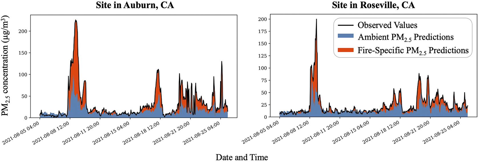
Figure 6. Ambient and fire-specific PM2.5 predictions 1 hour into the future from a temporal subset of testing results for example sites.
4. Prescribed fire simulations
A major contribution of this work is the novel framework integrating simulations of prescribed fires with GNN-based predictions of the resulting PM2.5 concentrations. The prescribed fires are simulated by transposing historical prescribed fires to target times. The Cal Fire (Cal Fire, Reference Firen.d.) latitude, longitude, and duration data for the prescribed burns are matched with the VIIRS FRP data. The transposed prescribed fire FRP information is combined with the observed meteorological data at the target times and input into the PM2.5-GNN model, which produces the PM2.5 predictions.
Using this framework, we perform two model experiments. Experiment 1 demonstrates how the PM2.5-GNN forecasting model can determine the optimal time to implement prescribed fires and focuses on the short-term pollution effect of prescribed fires. Experiment 2, on the other hand, focuses on quantifying the pollution impact of prescribed fires across months. In the rest of the section, we discuss each experiment in more detail:
4.1. Experiment 1: minimizing prescribed fire PM2.5 impact
4.1.1. Methods
To determine the optimal time to implement prescribed fires, we consider the immediate effect of prescribed fires. In effect, this experiment simulates historically prescribed fires and predicts the resulting PM2.5 pollution under different meteorological and fire conditions. That is, we transpose the FRP values from actual prescribed fire events to target time points and add them to the observed FRP values at those points. As these FRP values are combined, they are weighted using inverse distance and wind (both direction and magnitude), as outlined in Section 2.
In this experiment, we transpose a window of time containing prescribed fires (1/3/21–1/15/21) to target times throughout the year 2021 at 24-hour time steps to simulate the air quality impacts of controlled burns, as shown in Figure 7. This window contains 10 prescribed fires with burned areas above 100 acres.
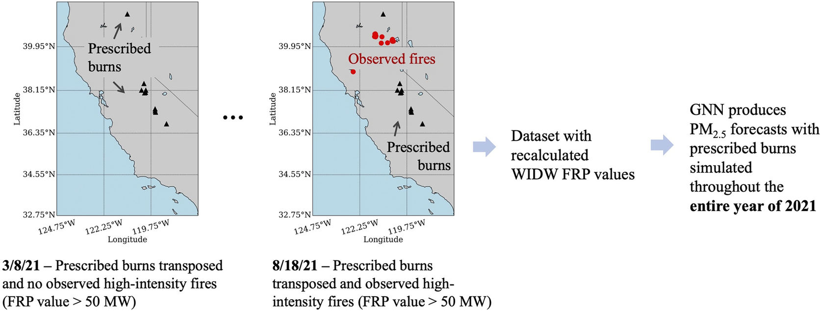
Figure 7. Schematic illustration of the methodology used in Experiment 1 to generate PM
 $ {}_{2.5} $
predictions based on simulated prescribed burns and observed fire events throughout 2021.
$ {}_{2.5} $
predictions based on simulated prescribed burns and observed fire events throughout 2021.
4.1.2. Results
As shown in Table 5, the month of August was the least optimal time to implement prescribed fires since it resulted in the most significant PM2.5 concentration. As August is during the peak wildfire season, implementing prescribed fires would only exacerbate the already hazardous air quality. August’s mean PM2.5 was 29.61% greater than the average mean of other months and August’s maximum was 44.27% greater than the average maximum of other months. On the other hand, March, which had the lowest mean value, was found to be the most optimal month to implement prescribed fires. The mean and maximum values were calculated by averaging the mean and maximum PM2.5 predictions of the locations whose PM2.5 observations were
 $ \ge $
50 μg/m3 during the window 1/3/21–1/15/21. As the PM2.5 observations at those locations were elevated during 1/3/21–1/15/21, they were likely influenced by the fire events transposed across the year 2021.
$ \ge $
50 μg/m3 during the window 1/3/21–1/15/21. As the PM2.5 observations at those locations were elevated during 1/3/21–1/15/21, they were likely influenced by the fire events transposed across the year 2021.
Table 5. Comparing the results of PM2.5 predictions based on simulated prescribed fires in Experiment 1 (see text for more details) for each month of 2021

4.2. Experiment 2: quantifying prescribed fire PM2.5 trade-off
4.2.1. Methods
This idealized experiment aims to quantify the pollution trade-off of implementing larger prescribed fires to mitigate emissions from the Caldor Fire, one of the largest Californian wildfires in 2021. Specifically, we use the PM2.5-GNN model to simulate the counterfactual scenario of performing scaled-up controlled burns in 2021 at the location of the Caldor Fire as shown in Figure 8. We employ two simulation techniques: one corresponding to the immediate air quality impact of more intense prescribed fires and the other to the longer-term effect of prescribed burning, related to mitigating the emissions from a larger wildfire such as the Caldor Fire.

Figure 8. Schematic illustration of the methodology used in Experiment 2 for simulating prescribed burns during spring and the absence of the Caldor Fire during the wildfire season.
For the first case, we simulated the effect of three historical prescribed fires, which were all within 20 km of the 2021 Caldor Fire, were active from 3/21 to 5/31 in 2018, 2019, and 2020, respectively, and burned around 6300 acres each. Since the Caldor Fire burned around 221,835 acres (Cal Fire, Reference Firen.d.), we assume that preventing a fire of that scale would require a larger controlled burn. Thus, when creating the fire-related input predictors, the FRP values from the prescribed fires are artificially increased by a factor of 100 and transposed together to 2021, thereby simulating large prescribed fires from 3/21/21 to 5/31/21. As described in Section 4.1, the prescribed fires are transposed by combining the FRP values of the prescribed fires with the observed FRP values from other fires at the target time point, followed by aggregating those values using inverse distance weighting and wind information.
In the latter case, we simulate the effect of controlled burns later in the year by excluding all FRP values within 25 km of the Caldor Fire between 8/14/21 and 10/21/21, assuming that a prescribed fire implemented earlier in the year (or even during the previous one to two fire seasons) could effectively mitigate a large fire in the same location a few months later. Since we use PM2.5 observations from the previous 10 days to initialize each 48-hour window of PM2.5 predictions, using the PM2.5 data from 2021 would implicitly include the Caldor Fire’s influence. To avoid this bias in our counterfactual scenario, we used as input the average of PM2.5 observations on the same date and hour from 8/14 to 10/2 in 2017, 2018, 2019, and 2020. Thus, the inputs will be fire-influenced but do not include the impact of the Caldor Fire. Limitations of our methodology are discussed in Section 4.2.3.
The PM2.5 predictions from this experiment’s counterfactual scenario are compared to baseline predictions derived using observed meteorological and fire inputs from 2021 without any prescribed fires around the Caldor Fire locations.
4.2.2. Results
The results support that although prescribed fires slightly increase PM2.5 in the short term, they reduce future PM2.5 resulting from wildfires. As shown in Table 6, the simulated prescribed burns led the mean of the PM2.5 predictions to be increased by an average of 0.31 μg/m3 and the maximum PM2.5 prediction to be increased by 3.07%. The mean and maximum values were calculated by averaging the mean and maximum PM2.5 predictions of the 13 PM2.5 monitor locations within 100 km of the Caldor Fire. Table 6 also quantifies that the maximum of the predictions with the Caldor Fire’s influence removed was 54.32% lower than the maximum of the baseline predictions. Thus, the magnitude of the immediate PM2.5 increase from the prescribed fire was significantly lower than the magnitude of the PM2.5 decrease experienced during the fire season. Furthermore, excluding the influence of the Caldor Fire reduced the number of days with an unhealthy daily average PM2.5 concentration from a mean of 3.54 days to 0.80 days. The reduction in PM2.5 pollution after excluding the Caldor Fire influence is illustrated in Figure 9, where the PM2.5 monitoring sites are color-coded depending on the PM2.5 pollution’s US AQI level.
Table 6. Comparing the predicted PM2.5 effect of simulated prescribed burns in Experiment 2 (see text for more details) with baseline PM2.5 predictions
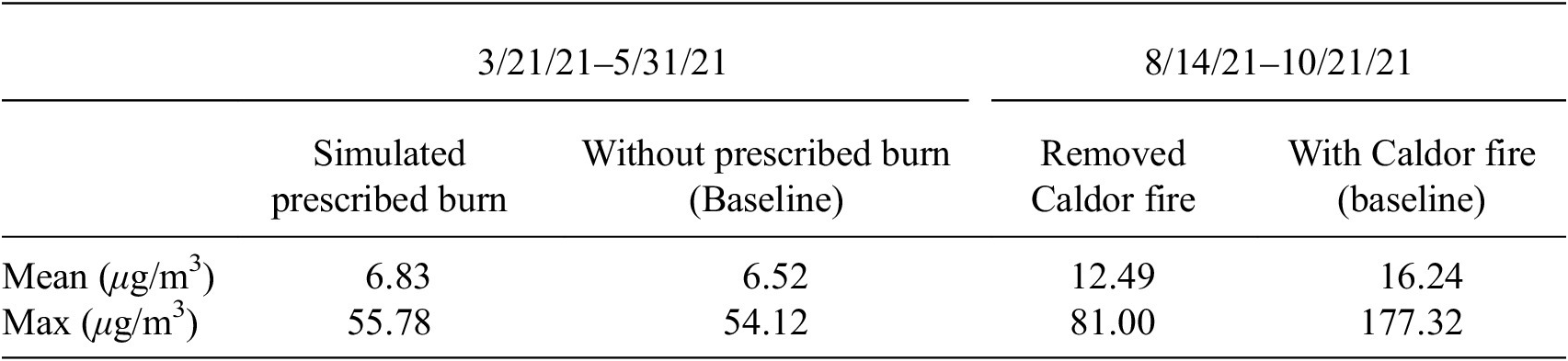

Figure 9. Maximum PM2.5 predictions per site from 8/14/21–12/31/21 under conditions (a) with prescribed burns at the Caldor Fire location during the spring and without Caldor Fire during the wildfire season and (b) without prescribed burns at the Caldor Fire location and with the Caldor Fire during the wildfire season.
4.2.3. Discussion
A limitation of our prescribed fire simulation methodology is the absence of ground truth PM2.5 data for counterfactual or simulated prescribed fire scenarios. This creates challenges in both defining PM2.5 inputs for the model and evaluating the accuracy of the simulation. Although no direct solution currently exists, our results can be compared to and validated against CTMs.
5. Conclusion and future work
This work generated hourly PM2.5 predictions for California using a PM2.5-GNN model and demonstrated that due to its spatio-temporal modeling capabilities, the PM2.5-GNN outperformed other machine learning models like the Random Forest, LSTM, and MLP. The temporally fine-grained, hourly PM2.5 predictions can help people better plan their outdoor activities to stay healthy. Additionally, our work focused on exploring two novel applications of the PM2.5-GNN model: (1) estimating the fire-specific contribution in PM2.5 forecasts and (2) predicting the PM2.5 for simulated fire events. Our work demonstrates the versatility of the PM2.5-GNN: the model can be applied to real-time prediction tasks, the GNN-based simulations from Experiment 1 can assess optimal windows for future prescribed fires, and the GNN-based simulations from Experiment 2 can be used for retrospective analysis.
Following previous machine learning-based studies (Aguilera et al., Reference Aguilera, Luo and Basu2023; Childs et al., Reference Childs, Li and Wen2022), we apply GNNs to the task of distinguishing the PM2.5 pollutant concentration emitted from fires versus ambient sources. This is significant as machine learning has higher computational efficiency than chemical transport models (CTMs) and the PM2.5-GNN model has been shown to outperform other machine learning models for pollution forecasting. Our hourly PM2.5-GNN predictions may also be a promising method to improve the skill of 2-day air quality forecasts. For the 48-hour prediction window that we considered here, the PM2.5-GNN model was shown to outperform other machine learning-based air quality forecasts due to its spatio-temporal inductive bias. Although we focused here on predictions at 112 sparse air quality sensor locations where there are historical PM2.5 measurements available, the PM2.5-GNN model has the ability to make predictions at sites that were not included in the original training dataset because of the spatiotemporal inductive bias of the PM2.5-GNN model.
To the best of our knowledge, this is the first research paper to apply machine learning for simulating the PM2.5 impact of prescribed fires, which is significant given the limitations of CTMs. A major contribution of this work is the prescribed fire simulation framework, which integrates prescribed fire simulations with GNN-based PM2.5 predictions. Future work will focus on improving the air quality simulations by incorporating fire risk models (Buch et al., Reference Buch, Williams and Juang2023; Langlois et al., Reference Langlois, Buch and Darbon2024) and physics-based smoke plume dynamics (Mallia and Kochanski, Reference Mallia and Kochanski2023) in the PM2.5-GNN model. Another promising direction is developing an auxiliary GNN model that incorporates the impact of individual fires and obviates the need to aggregate FRP values in the vicinity of each PM2.5 monitor, thereby making it easier to remove or add specific fire influences. Our framework provides land managers and the fire service with a useful tool to minimize the PM2.5 exposure of vulnerable populations, while also informing local communities of potential air quality impacts and beneficial trade-offs when implementing controlled burns.
Open peer review
To view the open peer review materials for this article, please visit http://doi.org/10.1017/eds.2025.4.
Author contribution
Conceptualization: Kyleen Liao; Jatan Buch; Kara Lamb; Pierre Gentine. Methodology: Kyleen Liao; Jatan Buch; Kara Lamb; Pierre Gentine. Data curation: Kyleen Liao. Data visualization: Kyleen Liao. Writing original draft: Kyleen Liao. All authors approved the final submitted draft.
Competing interest
None.
Data availability statement
Data and code for reproducing all the results can be found on GitHub: https://github.com/kyleenliao/PM2.5_Forecasting_GNN/tree/main
Funding statement
We acknowledge funding from NSF through the Learning the Earth with Artificial Intelligence and Physics (LEAP) Science and Technology Center (STC) (Award #2019625). Jatan Buch, Kara Lamb, and Pierre Gentine were also supported in part by the Zegar Family Foundation.
Ethical standard
The research meets all ethical guidelines, including adherence to the legal requirements of the study country.
A. Appendix
Comparing the heat maps of the baseline models in Figure 10 with those of the PM2.5-GNN in Figure 3 illustrates that the PM2.5-GNN performs best as indicated by the high
 $ {R}^2 $
values and density of points along the identity (y = x) line.
$ {R}^2 $
values and density of points along the identity (y = x) line.

Figure 10. Heat maps illustrating the observed versus predicted PM2.5 concentrations for 1-hour, 12-hour, and 48-hour forecasts, with log-transformed axes and color scale, for the Random Forest, LSTM, and MLP models. Also indicated are the identity line (dotted black) and
 $ {R}^2 $
values of the best-fit linear model.
$ {R}^2 $
values of the best-fit linear model.


 Open access
Comments
With climate change driving increasingly large and severe wildfires, dangerous levels of PM<sub>2.5</sub> pollution are being produced, posing significant health risks and causing millions of deaths annually. Our research applies machine learning to forecast PM<sub>2.5</sub> concentrations in California and estimate fire-specific PM<sub>2.5</sub> contributions.
Furthermore, our work quantifies the impact of prescribed burns, which while preventing wildfires also generate PM<sub>2.5</sub> pollution, leading to air quality concerns in nearby communities. To the best of our knowledge, our work is the first to use machine learning to predict the PM<sub>2.5</sub> concentrations from prescribed fires. We developed a novel framework and conducted experiments, which can assist the fire services in better understanding and minimizing the pollution exposure from prescribed fires.
We believe that our research is well-suited for publication in the Environmental Data Science (EDS) Special Collection for Tackling Climate Change with Machine Learning. Our work leverages machine learning to forecast PM<sub>2.5</sub> pollution during wildfires and prescribed burns, addressing both a critical environmental issue and a mechanism for its mitigation in a warmer, drier future.