Impact statement
There is a significant opportunity to reduce economic costs across a fleet of assets through optimization of the control policies under which assets operate. Reduction of economic costs is particularly important for high-value assets. A framework for the optimization of control policies is presented that considers both asset-level behavior and the fleet-level behavior that arises through the interaction between the assets. The framework is demonstrated for economic criteria relating to resource usage, component lifing, and maintenance scheduling, but is generically extensible. Results from a real-world case study are given that show the reduction in economic costs across a fleet of aerospace gas turbine engines. The framework has wide applicability, particularly in vehicular fleets such as aerospace, marine, and haulage industries as well as military fleets.
1. Introduction
An intelligent approach to the management of fleets can lead to a reduction in both operating costs and emissions while also increasing sustainability. Fleet management is particularly pertinent in the case of fleets containing complex, high-value assets with many degrees of freedom. Such assets tend to be expensive to operate and generate a large carbon footprint. The fleet management problem has been widely studied (Bielli et al., Reference Biell, Bielli and Rossi2011), examples include; vehicle routing (Bruglieri et al., Reference Bruglieri, Mancini, Pezzella and Pisacane2019), fleet composition (Yıldırım and Yıldız, Reference Yıldırım and Yıldız2021) and maintenance scheduling (Sanchez et al., Reference Sanchez, Boyacı and Zografos2020). In general, it is a challenging task, even in a static context, due to its combinatorial nature, that is combinations of behaviors across assets. The problem becomes more challenging when uncertainties such as future operation conditions, asset faults, resource availability, and uncertain future demands, are introduced.
One approach for fleet management is to use optimization routines to determine the optimal fleet behavior with respect to a set of objectives that represent an economic or environmental (or both) cost. Different problem formulations aim to optimize fleet behavior with respect to different costs, for example; increased fleet availability (Gavranis and Kozanidis, Reference Gavranis and Kozanidis2015; Vos et al., Reference Vos, Peng, Lee and Wang2023), reduction of operational costs (List et al., Reference List, Wood, Nozick, Turnquist, Jones, Kjeldgaard and Lawton2003; Militão and Tirachini, Reference Militão and Tirachini2021), reduction of carbon emission (Sawik et al., Reference Sawik, Faulin and Pérez-Bernabeu2017; Sheng et al., Reference Sheng, Meng and Li2019), etc.
It is often not feasible to construct these optimization problems analytically due to the highly complex nature of modern engineering assets, leading to many works choosing to use simulation-based approaches (Turan et al., Reference Turan, Elsawah and Ryan2020) and digital twins of assets (Kraft and Kuntzagk, Reference Kraft and Kuntzagk2017).
A fleet commonly contains groups of similar assets, but which are unique with respect to their operational and build history, i.e., when, where, and how they have been operated, current health state, original manufacture variability, and so forth each asset has many control variables and operating parameters which influence how the asset operates, see Figure 1. In this paper, it is assumed that every asset has the same control variables. However, the proposed framework can handle assets with different control variables. The chosen configuration of the control variables, named the policy, may have a large degree of redundancy with respect to the output of the asset, but have significant implications on resource usage and component lifing–and therefore on the economy of operation. The term lifing refers to the estimation of the remaining useful life of an asset or component. Due to the unique state of each asset and operating parameters, the optimal policy choice is different for each asset and may be constrained by external elements such as commercial contracts, operation costs, acceptable failure rates, asset maintenance, etc.

Figure 1. Interaction between elements in fleet operation.
The problem of finding optimal policies to extend the life of the assets, across these degrees of freedom, has been previously investigated at the asset level (Zheng et al., Reference Zheng, Zhang, Miao and Sun2017; Chen and Guo, Reference Chen and Guo2007). However, these solutions do not consider economic benefits that can be made at the fleet level. At the fleet level, the solution needs to consider the current state of all the assets and their interactions. For example, naively extending the life of multiple assets may lead to low availability or high maintenance shop occupancy during a later period. The optimal solution at the asset level may therefore be sub-optimal at the fleet level. Moreover, trade-offs between different objectives at the fleet level might exist. Performing the optimization at the fleet level has the potential to make significant economic and environmental savings but, to the best of the authors’ knowledge, has not been addressed in the existing literature.
In this work, we present a computationally tractable framework for fleet-level optimal policy selection. The proposed framework, referred to as an economic-based controller, generates optimal control policies for each of the fleet’s assets that improve expected life across the fleet while reducing operating costs and satisfying constraints such as fleet availability and maintenance shop capacity. The developed approach is demonstrated using a real-world case study targeting the optimal operation of a fleet of aerospace gas turbine engines. Asset lifing models are developed to find the relationship between policies and lifing. A fleet-level model is also developed and used to capture fleet-level behaviors. We demonstrate how such models can be used within common optimization frameworks to provide optimal solutions to fleet-level economic control. The main contributions of the proposed approach are: (1) a framework for economic policy optimization at the fleet level, (2) an approach for direct optimization of lifing models that remove the need for discrete event simulation of rare events, and (3) a demonstration of the developed methods in a real-world case study.
2. Fleet optimization
In this paper, we aim to find the optimal control policies across a fleet of complex assets. By finding an optimal policy for each asset, and considering their interactions, economic benefits can be obtained at the fleet level. Optimal policies can be found to increase the availability of the assets, restrict the number of assets simultaneously under maintenance, and so forth For example, for an asset close to planned maintenance, where a subset of its components are to be replaced, a control policy might be selected that can improve the asset performance at the cost of severe component usage–in order to exploit the otherwise wasted remaining life of these components. Alternatively, the fleet-level objective might encourage the selection of a policy that extends the maintenance interval in order to maintain workshop capacity. We are interested in minimizing multiple objectives such as reducing the probability of failure or minimizing the total fuel burn. A multi-objective optimization problem is therefore considered.
2.1. Problem definition
The problem is to find a set of policies for each of the
![]() $ H $
assets,
$ H $
assets,
![]() $ \boldsymbol{X}=\left\{{\boldsymbol{x}}_1,{\boldsymbol{x}}_2,\cdots, {\boldsymbol{x}}_H\right\} $
, where
$ \boldsymbol{X}=\left\{{\boldsymbol{x}}_1,{\boldsymbol{x}}_2,\cdots, {\boldsymbol{x}}_H\right\} $
, where
![]() $ {\boldsymbol{x}}_h=\left[{x}_{h,1},{x}_{h,2},\cdots, {x}_{h,M}\right] $
is the policy for the
$ {\boldsymbol{x}}_h=\left[{x}_{h,1},{x}_{h,2},\cdots, {x}_{h,M}\right] $
is the policy for the
![]() $ h $
’th asset which possesses
$ h $
’th asset which possesses
![]() $ M $
settings of the control system. The control setting
$ M $
settings of the control system. The control setting
![]() $ {x}_{h,m} $
could be, for example, an indexed control scheme or control parameterization, a control objective, or a valve state.
$ {x}_{h,m} $
could be, for example, an indexed control scheme or control parameterization, a control objective, or a valve state.
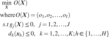
In order to optimize for multiple competing objectives at a different level, a multi-objective optimization problem is considered. The problem is formulated as:
 $$ {\displaystyle \begin{array}{l}\hskip0.36em \underset{\boldsymbol{X}}{\min}\hskip0.36em O\left(\boldsymbol{X}\right)\\ {}\mathrm{where}\;O\left(\boldsymbol{X}\right)=\left({o}_1,{o}_2,\dots, {o}_I\right)\\ {}\hskip0.72em s.t\hskip0.24em {g}_j\left(\boldsymbol{X}\right)\le 0,\hskip1em j=1,2,\dots, J\;\\ {}\hskip2.24em {d}_k\left({\boldsymbol{x}}_h\right)\le 0,\hskip1em k=1,2,\dots, K;h\in \left\{1,\dots, H\right\}\end{array}} $$
where
![]() $ {o}_i\left(\boldsymbol{X}\right) $
is
$ {o}_i\left(\boldsymbol{X}\right) $
is
![]() $ i $
’th objective function,
$ i $
’th objective function,
![]() $ {g}_j\left(\boldsymbol{X}\right) $
is
$ {g}_j\left(\boldsymbol{X}\right) $
is
![]() $ j $
’th fleet-level constraint,
$ j $
’th fleet-level constraint,
![]() $ {d}_k\left({\boldsymbol{x}}_h\right) $
is
$ {d}_k\left({\boldsymbol{x}}_h\right) $
is
![]() $ k $
’th asset level constraint and
$ k $
’th asset level constraint and
![]() $ I $
,
$ I $
,
![]() $ J $
, and
$ J $
, and
![]() $ K $
are the number of objective functions, fleet-level constraints, and asset-level constraints, respectively.
$ K $
are the number of objective functions, fleet-level constraints, and asset-level constraints, respectively.
The problem formulation is generic and accepts different types of objectives and constraints. Here, the objective is chosen with an aim to reduce economic costs through extending the life of the assets while minimizing resource usage under constraints on asset availability. As such, we consider an objective function of the form:
where
 $$ R\left(\boldsymbol{X}\right)=\frac{1}{H}\sum \limits_{h=1}^Hr\left({\boldsymbol{x}}_h\right), $$
 $$ L\left(\boldsymbol{X}\right)=-\frac{1}{H}\sum \limits_{h=1}^Hl\left({\boldsymbol{x}}_h\right), $$
 $$ {P}_{\mathrm{fail}}\left(\boldsymbol{X}\right)=\frac{1}{H}\sum \limits_{h=1}^HP\left({T}_{\mathrm{fail},h}<{T}_{L,h}\left({\boldsymbol{x}}_h\right)\right), $$
 $$ W\left(\boldsymbol{X}\right)=\frac{1}{H}\sum \limits_{h=1}^Hw\left({\boldsymbol{x}}_h,s\right), $$
where
![]() $ r\left({\boldsymbol{x}}_h\right) $
is a function that quantifies resource usage of the
$ r\left({\boldsymbol{x}}_h\right) $
is a function that quantifies resource usage of the
![]() $ h $
’th asset,
$ h $
’th asset,
![]() $ l\left({\boldsymbol{x}}_h\right) $
is a function that quantifies a lifing cost associate with component usage/degradation,
$ l\left({\boldsymbol{x}}_h\right) $
is a function that quantifies a lifing cost associate with component usage/degradation,
![]() $ {T}_{L,h}\left({\boldsymbol{x}}_h\right) $
is the usage limit (or hard life) of the
$ {T}_{L,h}\left({\boldsymbol{x}}_h\right) $
is the usage limit (or hard life) of the
![]() $ h $
’th asset (defined as the time at which the asset must be removed for maintenance as defined by the manufacturer or regulatory body),
$ h $
’th asset (defined as the time at which the asset must be removed for maintenance as defined by the manufacturer or regulatory body),
![]() $ {T}_{\mathrm{fail},h} $
is the failure time of the
$ {T}_{\mathrm{fail},h} $
is the failure time of the
![]() $ h $
’th asset,
$ h $
’th asset,
![]() $ w\left({\boldsymbol{x}}_h,s\right) $
is a function that quantifies economic costs associated with asset maintenance and depends on the state of the maintenance shop
$ w\left({\boldsymbol{x}}_h,s\right) $
is a function that quantifies economic costs associated with asset maintenance and depends on the state of the maintenance shop
![]() $ s $
. Maintenance costs could include the cost of replacement components, labor costs, or as demonstrated later, cost associated with occupancy. The objective function,
$ s $
. Maintenance costs could include the cost of replacement components, labor costs, or as demonstrated later, cost associated with occupancy. The objective function,
![]() $ O\left(\boldsymbol{X}\right) $
is therefore trying to minimize resource usage through
$ O\left(\boldsymbol{X}\right) $
is therefore trying to minimize resource usage through
![]() $ R\left(\boldsymbol{X}\right) $
, maximize asset life through
$ R\left(\boldsymbol{X}\right) $
, maximize asset life through
![]() $ L\left(\boldsymbol{X}\right) $
, minimize the the failure probabilities through
$ L\left(\boldsymbol{X}\right) $
, minimize the the failure probabilities through
![]() $ {P}_{\mathrm{fail}}\left(\boldsymbol{X}\right) $
and reduce maintenance costs through
$ {P}_{\mathrm{fail}}\left(\boldsymbol{X}\right) $
and reduce maintenance costs through
![]() $ W\left(\boldsymbol{X}\right) $
.
$ W\left(\boldsymbol{X}\right) $
.
Note that the objective
![]() $ W\left(\boldsymbol{X}\right) $
may introduce a coupling between the assets such that the optimization cannot be performed solely at the asset level.
$ W\left(\boldsymbol{X}\right) $
may introduce a coupling between the assets such that the optimization cannot be performed solely at the asset level.
2.2. Optimization with fleet simulators
In this section, the use of a fleet simulator is introduced as well as an overview of the optimization method used. A fleet simulator is required in order to evaluate the effect of the policies,
![]() $ \boldsymbol{X} $
, on the objective
$ \boldsymbol{X} $
, on the objective
![]() $ O\left(\boldsymbol{X}\right) $
. The simulator must therefore be able to estimate resource usage and model lifing effects to estimate asset hard lives and probabilities of failure.
$ O\left(\boldsymbol{X}\right) $
. The simulator must therefore be able to estimate resource usage and model lifing effects to estimate asset hard lives and probabilities of failure.
Under competing objectives, it is not always possible to find a solution that minimizes all objectives simultaneously. The variability of the fleet and the external influences, e.g., the current fuel price, may influence the priority of each of the objectives, but these can be difficult to quantify into weights. Therefore, we require an approach that returns a set of non-dominated solutions, called the Pareto optimal set, so the decision maker has the option of selecting a solution according to the context.
Formally, a point
![]() $ {x}^{\ast}\in X $
is Pareto optimal if there does not exist another point,
$ {x}^{\ast}\in X $
is Pareto optimal if there does not exist another point,
![]() $ x\in X $
, such that
$ x\in X $
, such that
![]() $ {o}_i(x)\le {o}_i\left({x}^{\ast}\right) $
for all
$ {o}_i(x)\le {o}_i\left({x}^{\ast}\right) $
for all
![]() $ i\in \left\{1,2,\dots, I\right\} $
and
$ i\in \left\{1,2,\dots, I\right\} $
and
![]() $ {o}_i(x)<{o}_i\left({x}^{\ast}\right) $
for at least one objective function.
$ {o}_i(x)<{o}_i\left({x}^{\ast}\right) $
for at least one objective function.
Multiple methods have been proposed to solve the multi-objective optimization problem (Gunantara, Reference Gunantara2018). Here, a genetic algorithm (GA) is used since it is a generic approach commonly used for the optimization of complex systems because it does not require an analytical model, which in many cases is impractical to obtain. Moreover, we consider a lightweight objective model (instead of a discrete event simulator) which lowers the benefits of constructing an optimization approach that could exploit additional information such as the objective’s gradient.
A GA takes a set, or population, of possible solutions and recombines and mutates them iteratively to produce new solutions. At each iteration, each candidate solution, here, equivalent to a policy set
![]() $ \boldsymbol{X} $
, is assigned a fitness value based on the achieved objective function. The best candidates are given a higher probability of being used in the next iteration. In this manner, solutions iteratively “evolve” to generate better candidates until a stopping criterion, e.g., the maximum number of iterations or minimum improvement, is satisfied.
$ \boldsymbol{X} $
, is assigned a fitness value based on the achieved objective function. The best candidates are given a higher probability of being used in the next iteration. In this manner, solutions iteratively “evolve” to generate better candidates until a stopping criterion, e.g., the maximum number of iterations or minimum improvement, is satisfied.
To find an optimal solution, the GA evaluates the quality of all the candidate solutions (policies) by passing each of the policies to the fleet simulator. Figure 2 shows the interaction between the GA optimizer and the different modules of the fleet simulator. The optimizer passes a candidate solution
![]() $ X $
to the simulator (blue lines). Each of the modules returns an objective evaluation (green lines) or constraint (red lines) to the optimizer. The optimizer then generates a new set of candidate solutions and the process is repeated. A detailed description of fleet simulator modules is presented in Section 3.
$ X $
to the simulator (blue lines). Each of the modules returns an objective evaluation (green lines) or constraint (red lines) to the optimizer. The optimizer then generates a new set of candidate solutions and the process is repeated. A detailed description of fleet simulator modules is presented in Section 3.
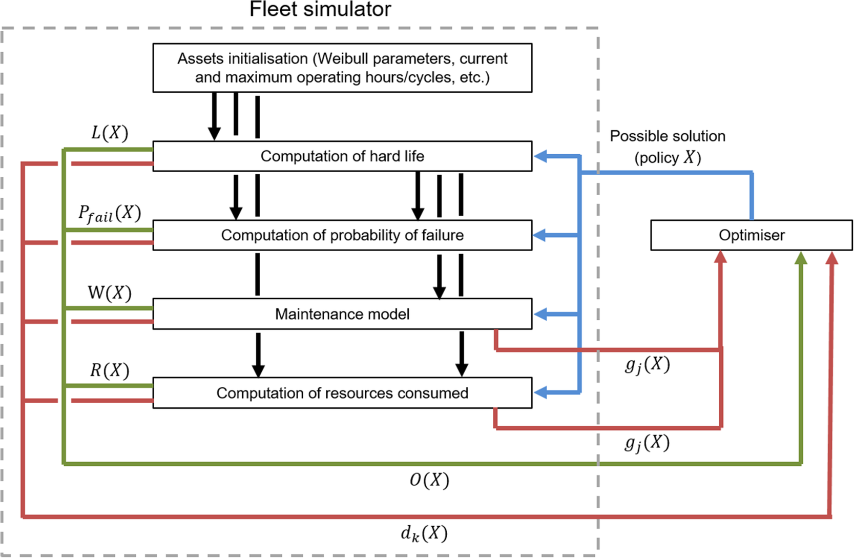
Figure 2. Interaction between optimizer and fleet simulator. The simulator’s modules receive a policy
![]() $ X $
from the optimizer. The modules return an objective evaluation and constraints that are used by the optimizer to assess the quality of the policy.
$ X $
from the optimizer. The modules return an objective evaluation and constraints that are used by the optimizer to assess the quality of the policy.
The optimal policies found after the optimization are based on the current condition of the fleet. A re-optimization is therefore required after an event that changes the fleet condition, e.g., asset maintenance or failure. After such an event, a new optimal policy for the whole fleet is computed under the new fleet condition by initializing the assets to reflect the new condition.
3. Asset life modeling
To understand the effects of different policies on the life of the asset, lifing models are required. Two aspects of asset lifing are considered. First, the usage limit of the asset,
![]() $ {T}_{L,h}\left(\boldsymbol{X}\right) $
, which we assume to be a function of the selected policy. Secondly, the asset’s probability of failure before its usage limit,
$ {T}_{L,h}\left(\boldsymbol{X}\right) $
, which we assume to be a function of the selected policy. Secondly, the asset’s probability of failure before its usage limit,
![]() $ {P}_{\mathrm{fail}}\left(\boldsymbol{X}\right) $
, which again is a function of the selected policy. In both cases, the mapping from the policy to the lifing effects is performed using a set of severity factors. In the remainder of this section, the estimation of severity factors under different policy choices is first described. This is followed by a description of how the severity factors can be used to evaluate the objectives
$ {P}_{\mathrm{fail}}\left(\boldsymbol{X}\right) $
, which again is a function of the selected policy. In both cases, the mapping from the policy to the lifing effects is performed using a set of severity factors. In the remainder of this section, the estimation of severity factors under different policy choices is first described. This is followed by a description of how the severity factors can be used to evaluate the objectives
![]() $ L\left(\boldsymbol{X}\right) $
and
$ L\left(\boldsymbol{X}\right) $
and
![]() $ {P}_{\mathrm{fail}}\left(\boldsymbol{X}\right) $
.
$ {P}_{\mathrm{fail}}\left(\boldsymbol{X}\right) $
.
3.1. Component life and severity factors
The set of severity factors associated with the
![]() $ h $
’th asset is defined as
$ h $
’th asset is defined as
![]() $ {\boldsymbol{c}}_h=\left[{c}_{1,h},{c}_{2,h},\dots, {c}_{N,h}\right] $
, where
$ {\boldsymbol{c}}_h=\left[{c}_{1,h},{c}_{2,h},\dots, {c}_{N,h}\right] $
, where
![]() $ N $
is the number of considered components belonging to the asset. The severity factors provide a mechanism to model changes in the life of the assets under different control policies. An overview of the procedure to compute the severity factors for different policies is presented below. It outlines a holistic framework that involves the asset performance calculation, models of the asset’s components, and computation of the oxidation, creep, and fatigue life.
$ N $
is the number of considered components belonging to the asset. The severity factors provide a mechanism to model changes in the life of the assets under different control policies. An overview of the procedure to compute the severity factors for different policies is presented below. It outlines a holistic framework that involves the asset performance calculation, models of the asset’s components, and computation of the oxidation, creep, and fatigue life.
Models of asset performance are used to simulate the asset performance under different operating conditions and policies. As shown in Figure 3, data from performance simulations under variable operating parameters are combined with thermal and mechanical damage models of individual components to perform a lifing analysis (1 and 2 in Figure 3). The analysis returns the damage suffered by each of the components (3 in Figure 3) which is compared to a reference mission to obtain a severity factor based on the policy used during the asset simulation. Coupling the performance and the lifing analysis process with an optimizer is complex and computationally expensive, if not infeasible in practice. For this reason, a Design of Experiment is performed with the policies as the independent variables, and the output performance and life consumption parameters are fitted to the analytical functions of the independent variables (4 in Figure 3). The data sets generated from the lifing analysis are used within a simple, yet novel, framework for the probabilistic modeling of system failure rates under different policies.
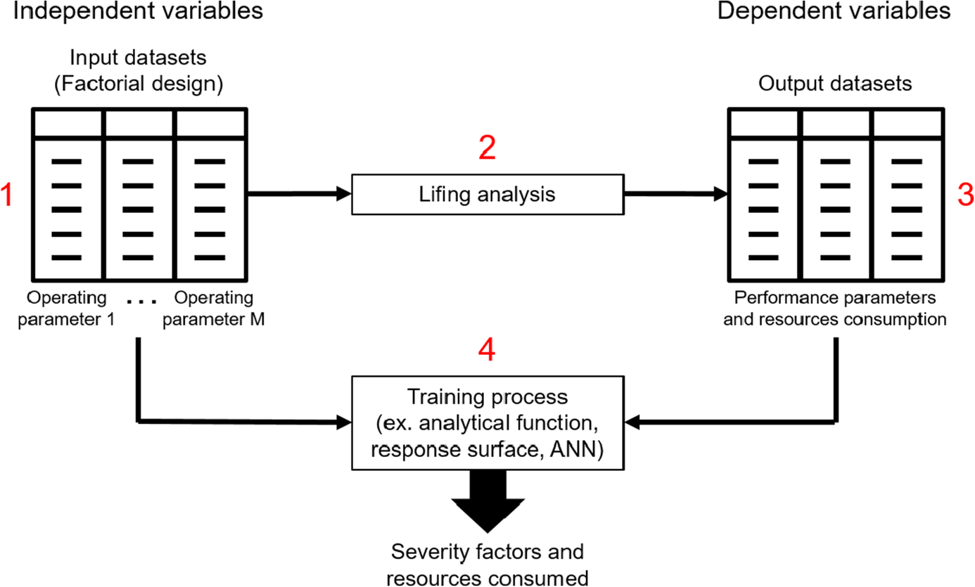
Figure 3. Computation of analytical models.
3.2. Time to maintenance model
The lifing characteristics of an asset or its sub-components can be described with a lifetime distribution. This approach is used in reliability engineering to describe the probability of failure, and other derived statistics, over a component’s life. The most commonly used lifetime distribution is the Weibull distribution due to its versatility and mathematical tractability (Life Data Analysis, Reference Analysis2024). These distributions can be obtained by fitting a statistical distribution to data collected during the asset’s operation under a nominal control policy. Here, Weibull analysis is extended to describe an asset comprised of a system of components with varying initial lives. The concept of component ‘severity’ is then introduced and it is shown how this acts on each component of the system through the parameters of the Weibull distribution.
As presented in Section 2.1, one optimization objective is to extend the life of the asset. That is, to increase the amount of operating hours available before a maintenance action is required. Maintenance is required in order to replace a subset of usage-limited components that reach the end of their life. Such components are termed life-limited components, and their life is defined in terms of a certain number of standard operating cycles or hours. The usage limit of the
![]() $ h $
’th asset must therefore be the minimum component usage limit for the components possessed by the assets,
$ h $
’th asset must therefore be the minimum component usage limit for the components possessed by the assets,
![]() $ {T}_{L,h}^0=\min \left\{{T}_{1,h}^0,{T}_{2,h}^0,\dots, {T}_{N,h}^0\right\} $
, where
$ {T}_{L,h}^0=\min \left\{{T}_{1,h}^0,{T}_{2,h}^0,\dots, {T}_{N,h}^0\right\} $
, where
![]() $ {T}_{i,h}^0 $
is the usage limit of the
$ {T}_{i,h}^0 $
is the usage limit of the
![]() $ i $
’th component of the
$ i $
’th component of the
![]() $ h $
’th asset. The severity factors are estimated such that they act as a multiplicative constant on the component usage limit, i.e.,
$ h $
’th asset. The severity factors are estimated such that they act as a multiplicative constant on the component usage limit, i.e.,
![]() $ {T}_i\left({c}_{i,h}\right)={c}_{i,h}{T}_i^0 $
. The asset usage limit is then given by;
$ {T}_i\left({c}_{i,h}\right)={c}_{i,h}{T}_i^0 $
. The asset usage limit is then given by;
3.3. Asset failure model
In this section, an expression for
![]() $ {P}_{\mathrm{fail}}\left(\boldsymbol{X}\right) $
is derived. Crucially, this formulation does not require Monte-Carlo simulation of a discrete event model in order to evaluate it, rather the probability is computed analytically allowing it to be directly minimized. The lifing characteristics of an asset or sub-component can be described with a lifetime distribution. This approach is used in reliability engineering to describe the probability of failure, and other derived statistics, over a component’s life. Weibull distributions are usually obtained by fitting to data collected during the asset’s operation or lifing analysis of individual components. Here, Weibull analysis is extended to describe an asset comprised of a system of components with varying initial lives. We make the assumption that component expected life changes depending on the policy and that this can be approximated using severity factors that act on each component through the parameters of the Weibull distribution.
$ {P}_{\mathrm{fail}}\left(\boldsymbol{X}\right) $
is derived. Crucially, this formulation does not require Monte-Carlo simulation of a discrete event model in order to evaluate it, rather the probability is computed analytically allowing it to be directly minimized. The lifing characteristics of an asset or sub-component can be described with a lifetime distribution. This approach is used in reliability engineering to describe the probability of failure, and other derived statistics, over a component’s life. Weibull distributions are usually obtained by fitting to data collected during the asset’s operation or lifing analysis of individual components. Here, Weibull analysis is extended to describe an asset comprised of a system of components with varying initial lives. We make the assumption that component expected life changes depending on the policy and that this can be approximated using severity factors that act on each component through the parameters of the Weibull distribution.
The probability density function of the Weibull distribution for the
![]() $ i $
’th component in the system is given by:
$ i $
’th component in the system is given by:
 $$ {f}_i(t)={f}_i\left(t|{k}_i,{\lambda}_i\right)=\frac{k_i}{\lambda_i}{\left(\frac{t}{\lambda_i}\right)}^{k_i-1}{e}^{-{\left(t/{\lambda}_i\right)}_i^k}, $$
for
![]() $ t\ge 0 $
, and
$ t\ge 0 $
, and
![]() $ 0 $
otherwise, where
$ 0 $
otherwise, where
![]() $ {\lambda}_i $
and
$ {\lambda}_i $
and
![]() $ {k}_i $
are the scale and shape parameters respectively.
$ {k}_i $
are the scale and shape parameters respectively.
![]() $ t $
is the time at which the Weibull is evaluated. This could be, for instance, the component life in hours or cycles.
$ t $
is the time at which the Weibull is evaluated. This could be, for instance, the component life in hours or cycles.
The cumulative distribution function for the
![]() $ i $
’th components in the system are
$ i $
’th components in the system are
It is also useful to define the survival function,
![]() $ {S}_i(z)=1-{F}_i(z) $
, which is the probability that the component
$ {S}_i(z)=1-{F}_i(z) $
, which is the probability that the component
![]() $ i $
survives beyond time
$ i $
survives beyond time
![]() $ z $
.
$ z $
.
To consider multiple components with non-zero initial lives, denoting the initial life of the
![]() $ i $
th component as
$ i $
th component as
![]() $ {z}_{i,0} $
, then, from Equation 9:
$ {z}_{i,0} $
, then, from Equation 9:
 $$ {F}_i^{\ast }(z)={\int}_{z_{i,0}}^{z+{z}_{i,0}}\frac{f_i(t)}{\int_{z_{i,0}}^{\mathrm{inf}}{f}_i(z) dz} dt $$
See Appendix F for a derivation of Equation 12.
Considering an asset comprised of a system of
![]() $ N $
components with varying initial lives,
$ N $
components with varying initial lives,
![]() $ {z}_{i,0} $
. The survival function of the system is:
$ {z}_{i,0} $
. The survival function of the system is:
 $$ {S}_{sys}(z)=\prod \limits_{i=1}^N\left[1-{F}_i(z)\right] $$
From Equations 12 and 14 the cumulative distribution of the system is described by:
where
![]() $ \boldsymbol{k}=\left[{k}_1,{k}_2,\dots, {k}_N\right] $
and
$ \boldsymbol{k}=\left[{k}_1,{k}_2,\dots, {k}_N\right] $
and
![]() $ \lambda =\left[{\lambda}_1,{\lambda}_2,\dots, {\lambda}_N\right] $
. The Weibull distribution has the useful property that, for a constant
$ \lambda =\left[{\lambda}_1,{\lambda}_2,\dots, {\lambda}_N\right] $
. The Weibull distribution has the useful property that, for a constant
![]() $ {c}_i $
:
$ {c}_i $
:
and this can be trivially extended to the system’s cumulative distribution function
This formulation of the cumulative distribution function provides a useful mechanism to model changes in the life of the asset under operating conditions and control policies that have different effects on the lifing characteristics of individual components. As can be seen from Equation 18, the severity factor acts as a multiplicative constant on the component’s expected failure time. It is used as the mechanism to modify the lifetime distributions based on the policy choice. The mapping between the policy and the severity factor is acquired by using first principles physics models of the component and is discussed in the next section.
By modifying the Weibull distribution based on a policy, i.e., applying different severity factors
![]() $ \boldsymbol{c} $
, the probability of failure for different policies can be computed. When rare and stochastic events associated with a low probability of failure are considered as objectives in an optimization problem, evaluating the effects of different policies can be challenging and might require thousands of simulations (Chen and Guo, Reference Chen and Guo2007). The computation of the probability of failure presented in this section is crucial to reducing the time required to solve the fleet optimization problem.
$ \boldsymbol{c} $
, the probability of failure for different policies can be computed. When rare and stochastic events associated with a low probability of failure are considered as objectives in an optimization problem, evaluating the effects of different policies can be challenging and might require thousands of simulations (Chen and Guo, Reference Chen and Guo2007). The computation of the probability of failure presented in this section is crucial to reducing the time required to solve the fleet optimization problem.
3.4. Maintenance model
A model of the maintenance process is required to estimate which components are replaced during maintenance based on the asset’s state. This procedure is entirely problem-specific and will depend on the cost of replacing components, the remaining life of all other components, the cost associated with workshop occupancy, and so forth The maintenance model also estimates the time required to repair the asset based on the state of the asset. This model is required to generate maintenance-based constraints as presented in Figure 2 and demonstrated in the next section.
4. Case study and results
The proposed approach is demonstrated using a real-world case study in which economic optimization for a fleet of aerospace gas turbine engines is performed. Gas turbine engines have many control variables and configurations that can be modified to affect their performance. They are subject to many constraints and external stimuli at the asset and fleet level, e.g., flight routes, contractually obliged maintenance, engine availability, and so forth By finding optimal control policies, that are specific to fleet operating conditions, we show that we can improve asset availability, i.e., reducing the time that assets are not available for use, while simultaneously reducing fuel burn.
The high-pressure turbine (HPT) of the modeled aerospace gas turbine engine (GTE) in this case study is temperature-regulated with independent cooling air valves. The setting of the cooling air valves are control variables that modulate the HPT blade cooling and, therefore, the HPT blade temperature. Increasing the level of cooling air decreases the blade temperature which reduces degradation through effects such as oxidation and creep. However, it requires air to be diverted from the main gas path causing an increase in gas path temperature and fuel burn to achieve the required thrust and therefore a decrease in the fuel efficiency. In the engine performance model, the cooling flow is simulated as high-pressure compressor (HPC) bleed air being mixed at the HPT inlet (for external cooling) and at the HPT outlet (for internal blade cooling) as shown in Figure 4. The amount of the modulated HPT internal blade cooling is then used in the blade temperature calculations and life consumption estimations as described by Pontika et al. (Reference Pontika, Laskaridis, Montana Gonzalez, Jacobs and Mills2023). The aim of this study is to find an optimal policy that defines a setting for the cooling air control variables across a fleet of engines. The level of cooling will affect the lives of the components of the HPT and the intermediate pressure turbine (IPT) differently depending on their location, material composition, etc., as well as the flight phase, e.g., take-off, climb, and cruise. Other components without active cooling, e.g., IPT blades, will be adversely affected by the rise in gas path temperature caused by the additional fuel burn. Therefore, a component-level model is important to assess the lifing impact of control policies with optimization results depending on the relative initial lives of all components. The optimizer finds a policy, for each engine, that sets control variables differently for each phase. Hence,
![]() $ \boldsymbol{X}\in {\mathrm{\mathbb{Z}}}^{M\times H} $
with
$ \boldsymbol{X}\in {\mathrm{\mathbb{Z}}}^{M\times H} $
with
![]() $ M=3 $
. For this case, discrete decision variables are considered. A case with continuous decision variables is presented later.
$ M=3 $
. For this case, discrete decision variables are considered. A case with continuous decision variables is presented later.
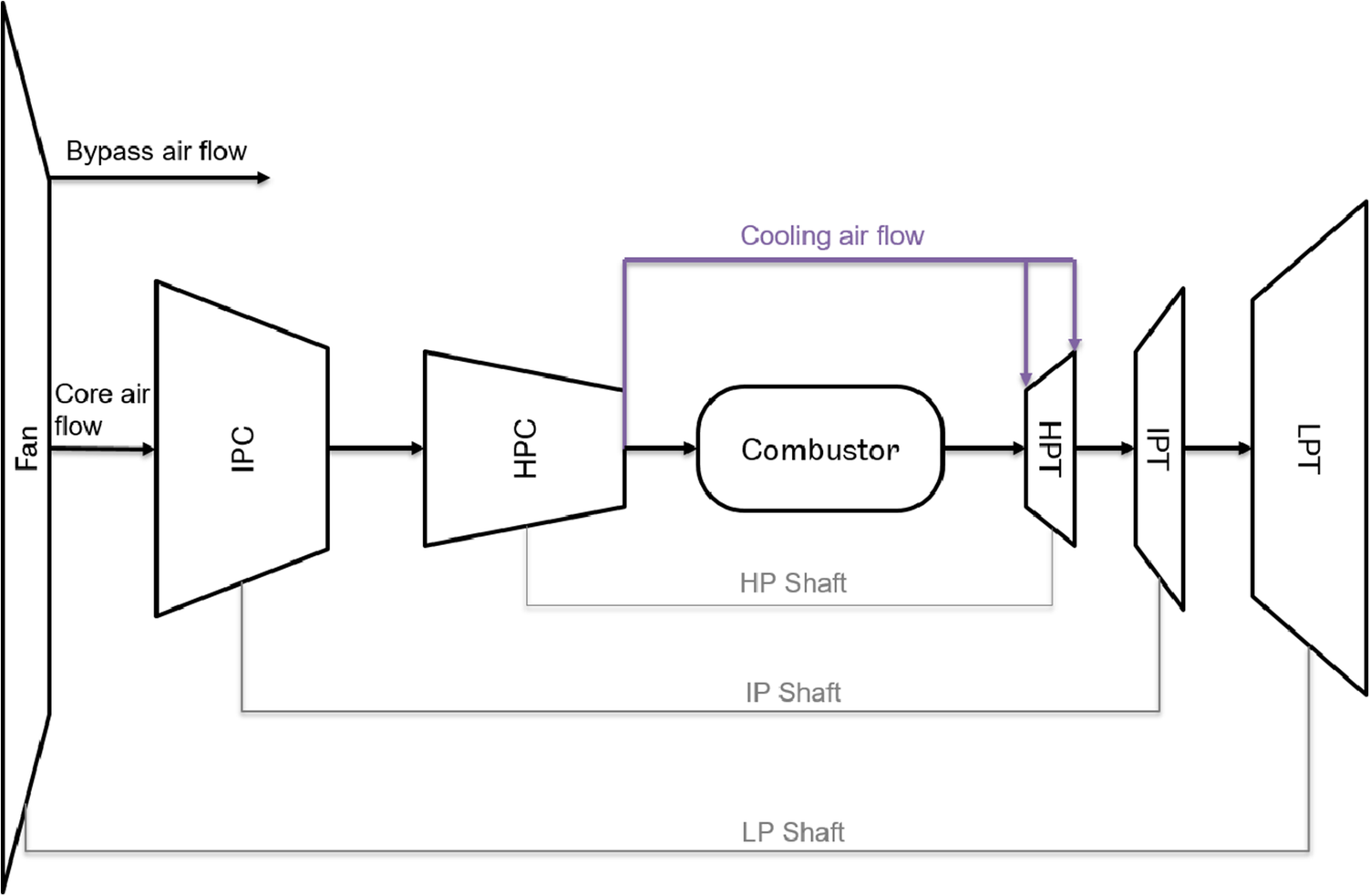
Figure 4. Illustration of cooling flow applied to the high-pressure turbine in the engine performance model. Air from the high-pressure compressor (HPC) is diverted to the high-pressure turbine (HPT).
4.1. GTE modeling
The engine performance modeling under variable policies is performed in Turbomatch (Giannakakis et al., Reference Giannakakis, Laskaridis, Nikolaidis and Kalfas2015; Macmillan, Reference Macmillan1974), an in-house component-based gas turbine performance simulation tool at Cranfield University. The aircraft performance and flight analysis, including the mission fuel burn, is performed in Hermes (Laskaridis et al., Reference Laskaridis, Pilidis and Kotsiopoulos2005), another in-house aircraft performance tool, which is coupled with Turbomatch to obtain the engine performance analysis. A generic three-spool turbofan engine model and a typical long-range wide-body aircraft model are considered. The Larson-Miller Parameter (Schneider et al., Reference Schneider, Mughrabi and Hammer1992) and Basquin/Coffing-Manson (Fuchs, Reference Fuchs1981) models together with the Arrhenius equation (Meier et al., Reference Meier, Nissley, Sheffler and Cruse1991) are used to calculate the effects of policies on the engine components’ lives and estimate the severity factors. An overview of the process is shown in Figure 5A and the interested reader is referred to Pontika et al. (Reference Pontika, Laskaridis, Montana Gonzalez, Jacobs and Mills2023) for a detailed description. The result of the modeling is a mapping between the policy and the severity factor and fuel burn in the form of a look-up table, graphed in Figure 5B. This mapping shows the sensitivity of the fuel burn and HPT/IPT severities to the different control variables. For example, it can be seen that the fuel consumption is highly sensitive to the cooling flow during cruise and relatively insensitive during take-off and climb.
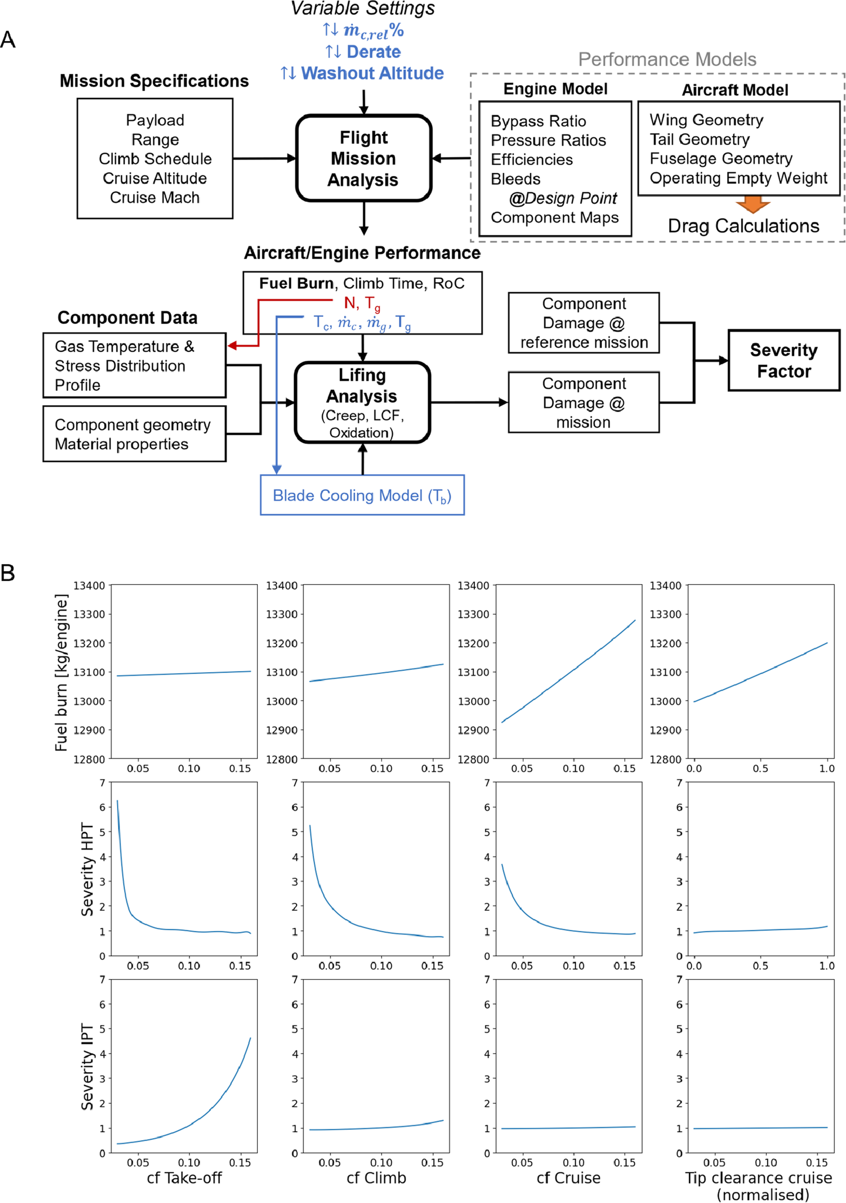
Figure 5. Estimation of severity factors. (A) Framework for performance and lifing analysis of future advanced aerospace engines. (B) Effects of cooling flow (cf) and tip clearance change at take-off, climb, and cruise.
4.2. Life of components and fuel trade-off
There is a trade-off between fuel consumption and the component life usage. Therefore, a Pareto front can be found from which a user can select a desirable policy for each of the engines. A fleet-level objective function is chosen which consists of the mean probability of failure (before maintenance) and mean fuel consumption across the fleet:
 $$ R\left(\boldsymbol{X}\right)=\frac{1}{H}\sum \limits_{h=1}^H\sum \limits_{m=1}^M{FC}_m\left({\boldsymbol{c}}_h\right), $$
 $$ {P}_{\mathrm{fail}}\left(\boldsymbol{X}\right)=\frac{1}{H}\sum \limits_{h=1}^H{F}_{sys}\left({T}_{L,h}\left({\boldsymbol{c}}_h\right)|{\boldsymbol{c}}_h,{\boldsymbol{k}}_h,{\boldsymbol{\lambda}}_h\right) $$
where
![]() $ H=50 $
and the function
$ H=50 $
and the function
![]() $ {FC}_m $
is a function that estimates the fuel consumption over the
$ {FC}_m $
is a function that estimates the fuel consumption over the
![]() $ m $
’th flight phase under policy
$ m $
’th flight phase under policy
![]() $ {\boldsymbol{x}}_h $
obtained through the framework presented in Section 3.1 and with the relationship shown in Figure 5B. The severity factors
$ {\boldsymbol{x}}_h $
obtained through the framework presented in Section 3.1 and with the relationship shown in Figure 5B. The severity factors
![]() $ {\boldsymbol{c}}_h $
and hence the asset’s hard lives
$ {\boldsymbol{c}}_h $
and hence the asset’s hard lives
![]() $ {T}_{L,h}\left({\boldsymbol{c}}_h\right) $
are implicitly a function of the policy
$ {T}_{L,h}\left({\boldsymbol{c}}_h\right) $
are implicitly a function of the policy
![]() $ {\boldsymbol{x}}_h $
. The probability of failure
$ {\boldsymbol{x}}_h $
. The probability of failure
![]() $ {P}_{\mathrm{fail}}\left(\boldsymbol{X}\right) $
is derived from Equation 18. Reducing the probability of engine maintenance through
$ {P}_{\mathrm{fail}}\left(\boldsymbol{X}\right) $
is derived from Equation 18. Reducing the probability of engine maintenance through
![]() $ {P}_{\mathrm{fail}}\left(\boldsymbol{X}\right) $
also reduces the cost associated with wasted life components replaced during maintenance. For simplicity, we therefore choose to exclude
$ {P}_{\mathrm{fail}}\left(\boldsymbol{X}\right) $
also reduces the cost associated with wasted life components replaced during maintenance. For simplicity, we therefore choose to exclude
![]() $ L\left(\boldsymbol{X}\right) $
from the cost. Objectives based on maintenance are considered in the next section. These objectives are computed by using the fleet simulator presented in Section 2.2. The fleet simulator was validated against a proprietary agent-based discrete event simulator provided by our industrial collaborator.
$ L\left(\boldsymbol{X}\right) $
from the cost. Objectives based on maintenance are considered in the next section. These objectives are computed by using the fleet simulator presented in Section 2.2. The fleet simulator was validated against a proprietary agent-based discrete event simulator provided by our industrial collaborator.
The agent-based discrete event simulator is tuned heuristically by subject matter experts with real data from gas turbine engines. A high-level description is now presented. The simulator starts by initializing every asset of the fleet. This initialization considers the type of components, e.g., model, of each asset and their initial life. After the initialization, information about the control policy to be applied and the conditions in which each asset is going to operate, e.g., route, is used to compute the maximum number of hours before maintanance (hard life). Then, given an operating schedule for each asset, e.g., number of hours to be operated, the life of the assets is simulated until maintance is required. The resources consumed until that point and the time required to repair the asset are computed. During maintenance, the model of the components can change based on an scheduled campaign. Therefore, the simulator updates the information of each repaired asset before repeating the process described above.
Our simulator, used for optimization problems in this section, runs 600 times faster than the proprietary software, allowing optimization within a reasonable time frame. The Python toolbox Pymoo (Blank and Deb, Reference Blank and Deb2020) was used to perform the optimization. Specifically, the non-dominated sorting GA NSGA-III (Deb and Jain, Reference Deb and Jain2013), which is efficient for many-objective optimization problems, was used. The solution is found in approximately 340 seconds on a laptop with a 2.30 GHz processor i7 and 16 GB of RAM. The stopping criterion is based on a threshold for objective improvement.
In the obtained Pareto front, each point represents a policy set for the whole fleet, i.e., a possibly different policy for each engine and each flight phase (take-off, climb, and cruise), see Figure 6A. In the Pareto front, the left-most and right-most policy sets are the solutions to the optimization problems with a single objective.
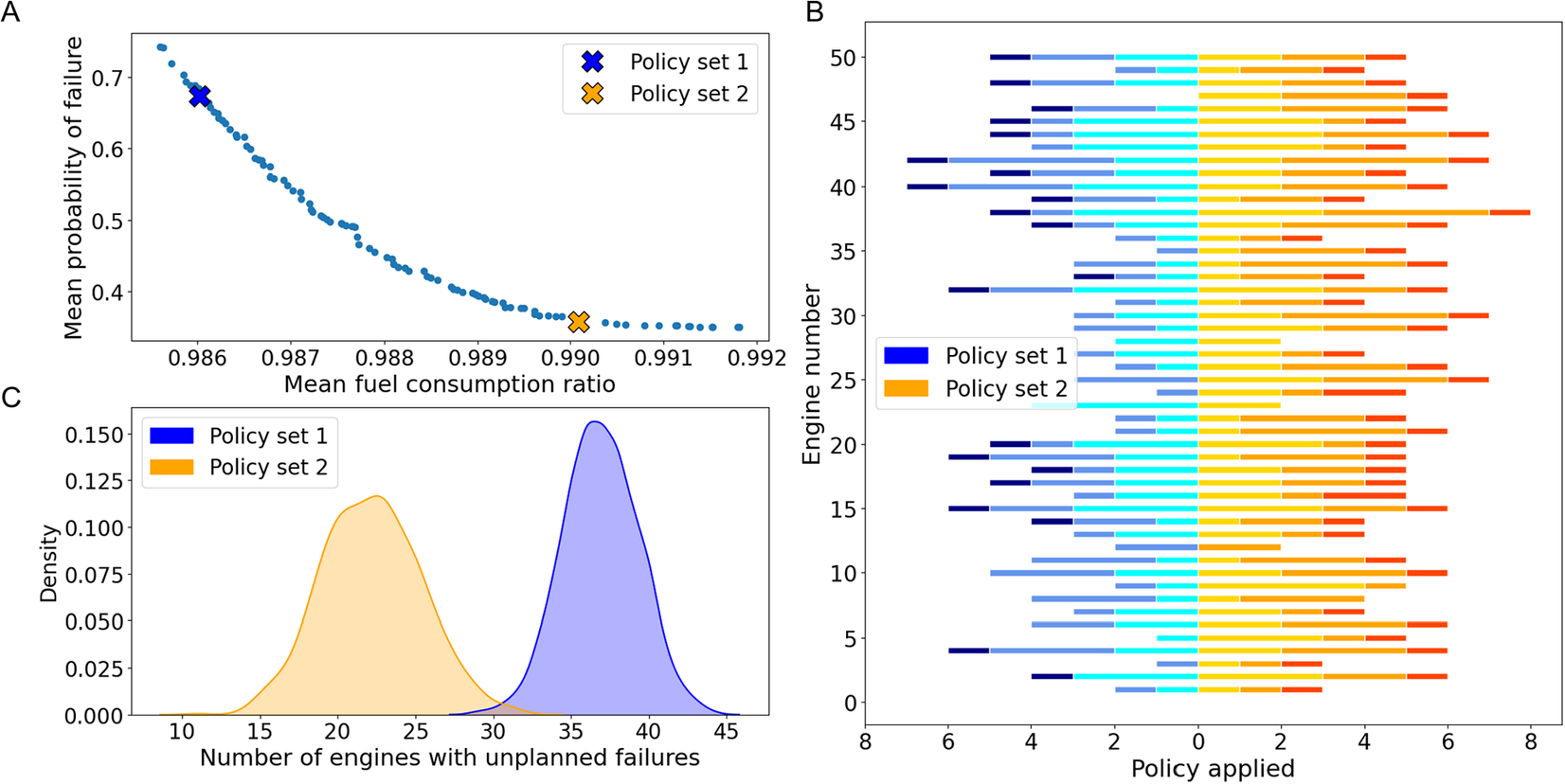
Figure 6. (A) Pareto front returned by the optimizer. A single solution can be selected by a user based on the current conditions. Policy set 1 can be selected to save fuel while policy set 2 reduces the probability of failure at the cost of higher fuel consumption. (B) Cooling flow levels applied to each engine. The stacked bars show the cooling flow level applied to each of the flight phases, i.e., take-off (light blue/orange), climb (blue/orange), and cruise (dark blue/orange). C) Distribution of unplanned failures after applying policies 1 and 2.
A user can select a single policy set, based on conditions such as fuel price, from the Pareto optimal policies returned by the optimizer. For instance, a policy that reduces the probability of failure at the cost of fuel consumption can be chosen when the fuel price is low. To demonstrate the effects of applying different policies, two policy sets are selected from the Pareto front. Policy set 1 is selected to reduce the fuel consumption across the fleet while policy set 2 is selected to reduce the probability of failure. The cooling flow levels for the selected policies are shown in Figure 6B. It is possible to see that, in general, higher levels of cooling are applied with policy set 2 to reduce the probability of failure. For example, for engine number 1, cooling flow is applied for only two phases (two bars) while for policy set 2 cooling flow is applied during every phase. The additional cooling flow has a negative effect on the fuel consumption, i.e., higher fuel consumption. To see how the selected policies affect the life of the engines, the policies are applied to the fleet in a Monte-Carlo simulation under the initial conditions used for the the optimization. The distribution of the number of engines that fail before their usage limit for each policy set is shown in Figure 6C. As expected, applying policy 2 reduces the number of unplanned failures at the cost of higher fuel consumption.
Note that because there are no constraints, the mean of the solutions obtained by solving the multi-objective optimization of each engine individually lies in the Pareto front presented in 6A. However, this is not true once constraints that affect the fleet are added to the problem as in the next section.
4.3. Maintenance scheduling
The results presented in the previous section do not consider any constraints. Besides constraints on the asset-level probability of failure and fuel consumption, constraints on the number of engines in the workshop can be considered with the proposed approach. These constraints can be used, for instance, to limit the simultaneous number of engines in the workshop (to conform to workshop capacity) or to increase the availability of engines during busy periods.
Recall that an engine is sent to the workshop when it reaches its usage limit, i.e., a maximum number of cycles. As presented in Section 3.2, some policies such as the cooling air can affect the component usage limit. Hence, it is possible to find policies where the number of engines in the workshop, within a period of time, is constrained. To satisfy such a constraint, the date when each engine would reach its usage limit, based on a policy, is computed by considering the flight schedules, i.e., the number of planned operating hours. The workshop model predicts the time required to repair the engine. This computation is performed during the fleet optimization cycle presented in Section 2.2. For this example, we aim to set the maximum number of engines in the workshop during July and August to zero, i.e.,
![]() $ {g}_1\left(\boldsymbol{X}\right)=S\left(\boldsymbol{X}\right)=0 $
, where
$ {g}_1\left(\boldsymbol{X}\right)=S\left(\boldsymbol{X}\right)=0 $
, where
![]() $ S\left(\boldsymbol{X}\right) $
is a function that returns the number of engines in a shop in this period. However, a better approach is to treat this constraint as an additional objective during the optimization to increase the number of feasible solutions. That is,
$ S\left(\boldsymbol{X}\right) $
is a function that returns the number of engines in a shop in this period. However, a better approach is to treat this constraint as an additional objective during the optimization to increase the number of feasible solutions. That is,
![]() $ W\left(\boldsymbol{X}\right)=S\left(\boldsymbol{X}\right) $
. This allows more solutions to be considered by relaxing the workshop requirement and increases the likelihood of finding feasible solutions. In addition, the probability of failure during the busy period can also be added as an objective to reduce the probability of unplanned maintenance during these months,
$ W\left(\boldsymbol{X}\right)=S\left(\boldsymbol{X}\right) $
. This allows more solutions to be considered by relaxing the workshop requirement and increases the likelihood of finding feasible solutions. In addition, the probability of failure during the busy period can also be added as an objective to reduce the probability of unplanned maintenance during these months,
![]() $ {\hat{P}}_{\mathrm{fail}}=P\left({T}_1<{T}_{\mathrm{fail},h}<{T}_2\right) $
, where
$ {\hat{P}}_{\mathrm{fail}}=P\left({T}_1<{T}_{\mathrm{fail},h}<{T}_2\right) $
, where
![]() $ {T}_1 $
and
$ {T}_1 $
and
![]() $ {T}_2 $
are the time points at the start and end of this period, i.e., start July and end August. Hence, in this example, we minimize
$ {T}_2 $
are the time points at the start and end of this period, i.e., start July and end August. Hence, in this example, we minimize
![]() $ O\left(\boldsymbol{X}\right)=\left(R,{P}_{\mathrm{fail}},W,{\hat{P}}_{\mathrm{fail}}\right) $
. Note that for this computation, the initial operating hours are considered from the beginning of the considered period, i.e., July.
$ O\left(\boldsymbol{X}\right)=\left(R,{P}_{\mathrm{fail}},W,{\hat{P}}_{\mathrm{fail}}\right) $
. Note that for this computation, the initial operating hours are considered from the beginning of the considered period, i.e., July.
To present the evaluated objectives for all the policies found during the constrained optimization, we use a parallel coordinate plot, see Figure 7A. In this plot, each color represents a policy set, i.e., a point in the 2D Pareto presented in Figure 6A. As in the previous case, the trade-off between probabilities of failure and fuel consumption can be observed. The result shows that it is not always possible to find optimal policies with zero maintenance during the busy period. Given these policy sets, the decision maker can select a set with an acceptable level of assets in maintenance if necessary.

Figure 7. (A) Parallel coordinate plot of Pareto front. (B) Maintenance dates for an optimal policy without constraints. (C) Maintenance of engines with a constraint on the number of engines in the workshop. Maintenance during the busy period (highlighted region) is avoided by repairing four engines early and three engines after this period. (D) Cooling flow level applied to each engine. The policies of the engines that are repaired during the busy period in the unconstrained problem are highlighted.
Figure 7B, C shows the number of engines in the workshop on different dates for two selected policies with similar fuel consumption, one for the unconstrained solution and the other for the constrained one. In the constrained solution, the optimizer returns policies that avoid the maintenance of engines during summer, see Figure 7D.
It is not always possible to find optimal policies with zero planned maintenance during a specific period, see Figure 7. To improve the flexibility of the obtained policies, an extra decision variable,
![]() $ {x}_e $
, representing early maintenance can be added to the optimization problem. By sending an engine to the workshop before its scheduled maintenance, based on the new decision variable, policies that satisfy tighter constraints can be found. Sending an engine to the workshop before its scheduled maintenance incurs an economic cost through, for example, wasted component life. For simplicity, we do not consider a specific cost, instead, the mean time before maintenance (in months) is considered in the cost function. This objective can be defined as
$ {x}_e $
, representing early maintenance can be added to the optimization problem. By sending an engine to the workshop before its scheduled maintenance, based on the new decision variable, policies that satisfy tighter constraints can be found. Sending an engine to the workshop before its scheduled maintenance incurs an economic cost through, for example, wasted component life. For simplicity, we do not consider a specific cost, instead, the mean time before maintenance (in months) is considered in the cost function. This objective can be defined as
![]() $ l\left({\boldsymbol{x}}_h\right)={\boldsymbol{x}}_{h,e} $
. Because the additional decision variable increases the number of policies where the number of engines in shop during the busy period is zero, we remove the objective
$ l\left({\boldsymbol{x}}_h\right)={\boldsymbol{x}}_{h,e} $
. Because the additional decision variable increases the number of policies where the number of engines in shop during the busy period is zero, we remove the objective
![]() $ W\left(\boldsymbol{X}\right) $
and add the constraint
$ W\left(\boldsymbol{X}\right) $
and add the constraint
![]() $ {g}_1\left(\boldsymbol{X}\right)=S\left(\boldsymbol{X}\right)=0 $
. Hence, the objectives considered in this example are
$ {g}_1\left(\boldsymbol{X}\right)=S\left(\boldsymbol{X}\right)=0 $
. Hence, the objectives considered in this example are
![]() $ O\left(\boldsymbol{X}\right)=\left(R,L,{P}_{\mathrm{fail}},{\hat{P}}_{\mathrm{fail}}\right) $
. Figure 8 shows the parallel coordinate of each solution obtained after the optimization. It is possible to see that, in contrast to the previous results, a richer set of policies that meet the condition of zero maintenance during the busy period is obtained.
$ O\left(\boldsymbol{X}\right)=\left(R,L,{P}_{\mathrm{fail}},{\hat{P}}_{\mathrm{fail}}\right) $
. Figure 8 shows the parallel coordinate of each solution obtained after the optimization. It is possible to see that, in contrast to the previous results, a richer set of policies that meet the condition of zero maintenance during the busy period is obtained.

Figure 8. Parallel coordinate plot of Pareto front obtained with an extra decision variable representing early maintenance. A rich set of policies that meet the condition of zero maintenance during the busy period are obtained.
The result in this section demonstrates that the proposed approach can be used for maintenance scheduling in two manners. Firstly, to find optimal policies given a predefined maintenance preference as demonstrated above. Secondly, to plan the maintenance after selecting a policy obtained from an unconstrained optimization.
4.4. Tip clearance control
This section presents how the proposed framework can be used for different control variables. Specifically, tip clearance is considered in addition to the cooling flow presented in the previous sections. Tip clearance is the radial distance between the blade tip of a turbine and the casing, see Figure 9. Increasing the tip clearance directly decreases the efficiency of the engine Holeski and Futral (Reference Holeski and Futral1969) resulting in higher fuel consumption. This is because the power that a turbine can provide depends on the airflow flow through the area where the blade is located. In the presented case study, the relative change in tip clearance is translated into a relative change in component efficiency using the empirical correlation provided by Kurzke and Halliwell (Reference Kurzke and Halliwell2018) for shrouded turbine blades.
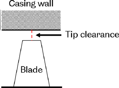
Figure 9. Illustration of the blade–casing clearance.
A small tip clearance is desirable to improve the engine efficiency but increases the risk of the turbine blade making contact with, and abrading, the case lining (shroud), named a tip rub event. The variable conditions under which the engine operates, e.g., variable temperatures, pressures, and vibration change the gap between the blade tip and the shroud (clearance) which changes the probability of a tip rub occurring. The abrasion of the shroud after the tip rub event permanently increases the tip clearance until the engine is repaired, see Figure 10. Hence, an engine will have a higher fuel consumption following a tip rub event. This suggests that there may be a benefit in applying a smaller tip clearance when the engine is nearing maintenance as the future loss of fuel efficiency is less. Tip clearance can be modulated by cooling the case, again using cooling air which is controlled using the turbine case cooling valve. Cooling the case causes it to contract which decreases the tip clearance. The tip clearance is controlled in a closed loop, the target clearance is a further control variable that can be added to the policy.

Figure 10. Illustration of the effect of tip rub event. The gap between the blades and the casing increases after a tip rub until the engine is repaired. This results in an increment in fuel consumption.
In addition to affecting fuel consumption, the tip clearance also affects the probability of failure. If an engine runs less efficiently, more power, and as a consequence, more heat is generated to reach the required operation point. Therefore, the life of the engine components is reduced. The gas turbine modeling presented in Section 4.1 was used to estimate the effects of the tip clearance in cruise and cooling flow in the fuel consumption and severity factors of the HPT and IPT. Given this model, three different problems were solved:
-
1. The decision variable of the
 $ {h}^{\prime } $
th engine,
 $ {x}_h $
, is defined as the change or delta in the tip clearance (compared to the tip clearance without control).
 -
2. The decision variable
 $ {\boldsymbol{x}}_h=\left[{x}_{h,1},{x}_{h,2},{x}_{h,3}\right] $
is defined as the cooling flow for each of the flight phases. This is equivalent to the problem solved in Section 4.2 but with continuous decision variables and the severity factor models obtained by modeling the effects of tip clearance and cooling flow.
 -
3. The decision variable
 $ {\boldsymbol{x}}_h=\left[{x}_{h,1},{x}_{h,2},\cdots, {x}_{h,4}\right] $
is defined as the delta of the tip clearance and the cooling flow for each of the flight phases.
For these problems, a fleet of 20 engines was considered. Moreover, no constraints were considered and the objection function presented in Section 4.2 was minimized.
The solution to the first problem is presented in Figure 11. As shown in Figure 11A, the tip clearance delta applied to the engine has a direct correlation with the time to maintenance. As presented above, this result is expected because the effect of a tip rub is minimized when the engine is closed to be repaired. Figure 11B shows how the fuel consumption is reduced as the tip clearance delta increases until it reaches a point where a tip rub happens. Because the tip clearance increases after this point, the efficiency of the engine is affected. This results in a higher fuel consumption. Because of the correlation between tip clearance and hours to maintenance, for this problem, a single optimal solution can be found.
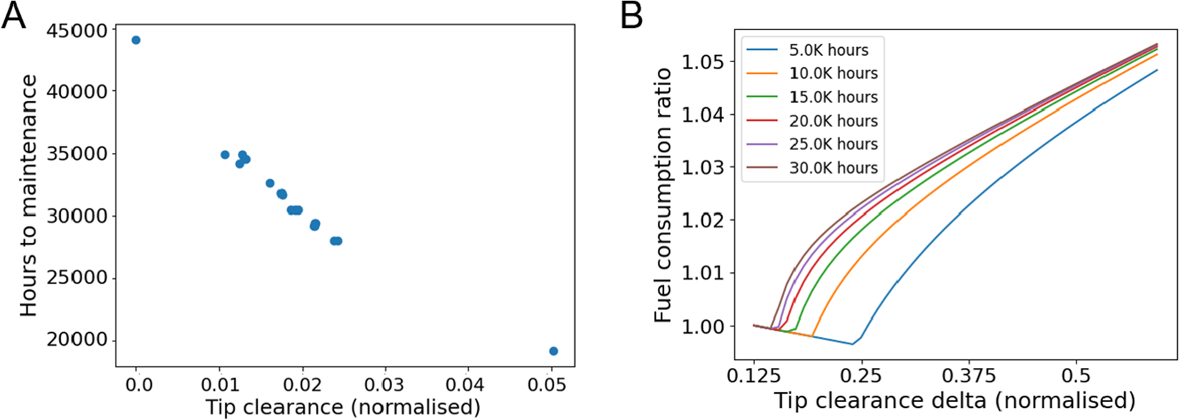
Figure 11. A: Tip clearance delta applied to the engines. B: Total fuel consumption before maintenance for different tip clearance policies.
The Pareto fronts for the second and third problems are presented in Figure 12. It is possible to see that the addition of an extra degree of freedom improves the solution obtained, i.e., a lower probability of failure and fuel consumption can be achieved.
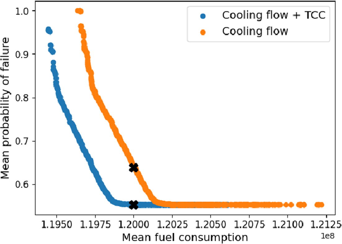
Figure 12. Pareto front returned by optimizer after solving the problem with tip clearance delta as decision variable and tip clearance with cooling flow, respectively. Two policy sets with similar fuel consumption are selected for comparison.
From these Pareto fronts, two policy sets are selected for comparison. This comparison can be seen in Figure 13. This figure shows that, in general, more cooling flow is applied to the engines when the tip clearance is also controlled. From Figure 5, it can be seen that as the cooling flow applied to the engine increases the fuel consumption also increases. On the other hand, the fuel consumption is reduced when a small tip clearance is applied. Therefore, by running an engine more efficiently (and reducing fuel consumption) by applying a tip clearance policy, more cooling flow can be applied without having high levels of fuel consumption. Therefore, more cooling flow can be applied compared to the case where the tip clearance is not changed.

Figure 13. Cooling flow policies applied to engines based on the the policy sets selected in 12.
When cooling flow and tip clearance are considered as a control policy, the clear correlation between hours to maintenance and tip clearance disappears, see Figure 14. Therefore, selecting an optimal policy without solving a multi-objective optimization problem is not trivial. Understanding what factors, e.g., route and component’s model, determine the optimal policies is future work.
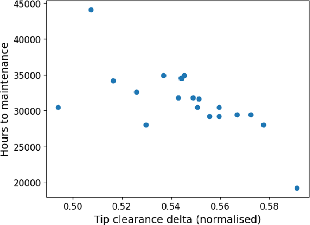
Figure 14. Tip clearance delta applied to the engines.
5. Conclusions
Fleet management has been widely studied in different settings due to its potential to reduce both operating costs and emissions while also increasing sustainability. This paper presents a novel framework for multi-objective fleet optimization to find optimal control policies with the objective of increasing the life of the fleet’s assets and/or minimizing the resources required for the fleet operation. The proposed framework consists of engine lifing models for mapping control policies to the life of engine components and a fleet model developed to reduce the number of simulations required to evaluate candidate solutions. Results show that based on the selected policy, the probability of unplanned maintenance or fuel consumption across the fleet can be reduced. Moreover, they show how, by considering constraints such as the maximum number of assets in maintenance during busy periods, the framework can be used to schedule the maintenance of the fleet assets. Different types of control policies as well as different optimization scenarios and constraints are considered in the examples to demonstrate the framework flexibility.
Data availability statement
To get access to research data, please contact one corresponding author.
Author contributions
Conceptualization: W.J, A.M; Data curation: F.M, M.G; Formal analysis: F.M, W.J; Funding acquisition: V.K, P.B, D.W, A.M, P.L; Investigation: F.M, E.P; Methodology: F.M, W.J, A.M, E.P; Project administration: P.B, D.W, V.K, A.M, P.L; Resources: M.G, P.B; Software: F.M, W.J; Supervision: W.J, P.B, D.W, A.M, P.L; Validation: F.M, W.J, M.G, A.M; Visualization: F.M, W.J, E.P; Writing original draft: F.M, W.J, E.P, A.M; Writing review & editing: F.M, A.M, E.P, V.K,
Funding statement
This research was supported by Innovate UK–113,263 PINES (2020). University of Sheffield Institutional Open Access Fund: for the purpose of open access, the author has applied a Creative Commons Attribution (CC BY) licence to any Author Accepted Manuscript version arising.
Competing interest
The authors declare no competing interests exist.
Ethical standards
The research meets all ethical guidelines, including adherence to the legal requirements of the study country.
Appendix 1
Derivation of Equation 12
 $$ {\displaystyle \begin{array}{c}{F}_0={\int}_{z_{i,0}}^{\infty }{f}_i(z)\; dz\\ {}={\int}_{z_{i,0}}^{\infty }{\left(\frac{z}{\lambda}\right)}^{k-1}{e}^{-{\left(\frac{z}{\lambda}\right)}^k}\; dz\end{array}} $$
making the substitution
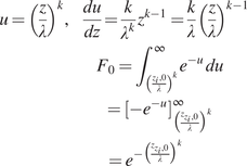 $$ {\displaystyle \begin{array}{l}u={\left(\frac{z}{\lambda}\right)}^k,\hskip1em \frac{du}{dz}=\frac{k}{\lambda^k}{z}^{k-1}=\frac{k}{\lambda }{\left(\frac{z}{\lambda}\right)}^{k-1}\\ {}\hskip9em {F}_0={\int}_{{\left(\frac{z_i,0}{\lambda}\right)}^k}^{\infty }{e}^{-u}\; du\\ {}\hskip10em ={\left[-{e}^{-u}\right]}_{{\left(\frac{z_{z_i,0}}{\lambda}\right)}^k}^{\infty}\\ {}\hskip10.12em ={e}^{-{\left(\frac{z_{z_i,0}}{\lambda}\right)}^k}\end{array}} $$
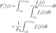 $$ {\displaystyle \begin{array}{c}{F}_i^{\ast }(z)={\int}_{z_{i,0}}^{z+{z}_{i,0}}\frac{f_i(t)}{\int_{z_{i,0}}^{\infty }{f}_i(z) dz}\; dt\\ {}=\frac{1}{F_0}{\int}_{z_{i,0}}^{z+{z}_{i,0}}{f}_i(t)\; dt\end{array}} $$
making the same substitution given in Equation 23
 $$ {\displaystyle \begin{array}{c}{F}_i^{\ast }(z)={e}^{{\left(\frac{z_{z_i,0}}{\lambda}\right)}^k}{\left[-{e}^{-u}\right]}_{{\left(\frac{z_{z_i,0}}{\lambda}\right)}^k}^{{\left(\frac{z+{z}_{x_i,0}}{\lambda}\right)}^k}\\ {}={e}^{{\left(\frac{z_{z_i,0}}{\lambda}\right)}^k}\left[-{e}^{-{\left(\frac{z+{z}_{z_i,0}}{\lambda}\right)}^k}+{e}^{-{\left(\frac{+{z}_{z_i,0}}{\lambda}\right)}^k}\right]\\ {}=1-{e}^{-{\left(\frac{z+{z}_{0,i}}{\lambda_i}\right)}^{k_i}+{\left(\frac{z_{0,i}}{\lambda_i}\right)}^{k_i}}\end{array}} $$


Comments
No Comments have been published for this article.