


1 Introduction
Electrical resistor networks are modeled by undirected graphs whose edges are given positive weights, and have been studied for two centuries. The physical axioms governing such networks, Ohm’s Law and Kirchhoff’s Law, were discovered in the 19th century. In the last few decades, planar resistor networks have been studied from a modern perspective in the works of Curtis–Ingerman–Morrow [Reference Curtis, Ingerman and MorrowCIM98], de Verdière–Gitler–Vertigan [Reference Colin de Verdière, Gitler and VertiganCdVGV96], Kenyon–Wilson [Reference Kenyon and WilsonKW11], Lam–Pylyavskyy [Reference Lam and PylyavskyyLP15], Lam [Reference LamLam18], Chepuri–George–Speyer [Reference Chepuri, George and SpeyerCGS21], and Bychkov–Gorbounov–Kazakov–Talalaev [Reference Bychkov, Gorbounov, Kazakov and TalalaevBGKT21], and others.
1.1 Grove coordinates
In Kirchhoff’s classical work, he gave formulae for the effective resistance of an electrical network by counting spanning trees. We formalize the tree enumeration in terms of groves [Reference Kenyon and WilsonKW11]. Let
 $\Gamma $
be a planar electrical network with n boundary nodes. A grove in
$\Gamma $
be a planar electrical network with n boundary nodes. A grove in
 $\Gamma $
is a spanning forest F such that every connected component contains a boundary node. Each grove has a noncrossing boundary partition
$\Gamma $
is a spanning forest F such that every connected component contains a boundary node. Each grove has a noncrossing boundary partition
 $\sigma (F)$
.
$\sigma (F)$
.
The grove coordinates
 $L_\sigma (\Gamma )$
count groves in
$L_\sigma (\Gamma )$
count groves in
 $\Gamma $
with chosen boundary partition
$\Gamma $
with chosen boundary partition
 $\sigma $
and determine
$\sigma $
and determine
 $\Gamma $
up to electrical equivalence (series–parallel and
$\Gamma $
up to electrical equivalence (series–parallel and
 $Y-\Delta $
moves). In [Reference LamLam18], the second author constructed a compactification of the space of planar electrical networks with n boundary vertices, using the grove coordinates
$Y-\Delta $
moves). In [Reference LamLam18], the second author constructed a compactification of the space of planar electrical networks with n boundary vertices, using the grove coordinates
 $(L_\sigma )$
. Furthermore, an embedding of this compactification into the Grassmannian
$(L_\sigma )$
. Furthermore, an embedding of this compactification into the Grassmannian
 $\operatorname {\mathrm {Gr}}(n-1,2n)$
is constructed; we denote the image of this compactification by
$\operatorname {\mathrm {Gr}}(n-1,2n)$
is constructed; we denote the image of this compactification by
 $\mathcal {X}_{n,\geq 0}$
and let
$\mathcal {X}_{n,\geq 0}$
and let
 $\mathcal {X}_n \subset \operatorname {\mathrm {Gr}}(n-1,2n)$
denote its Zariski-closure, an irreducible subvariety of the Grassmannian.
$\mathcal {X}_n \subset \operatorname {\mathrm {Gr}}(n-1,2n)$
denote its Zariski-closure, an irreducible subvariety of the Grassmannian.
The starting point of our work is the analogy between the Grassmannian
 $\operatorname {\mathrm {Gr}}(k,n)$
and the variety
$\operatorname {\mathrm {Gr}}(k,n)$
and the variety
 $\mathcal {X}_n$
, and between the Plücker coordinates
$\mathcal {X}_n$
, and between the Plücker coordinates
 $\Delta _I$
and the grove coordinates
$\Delta _I$
and the grove coordinates
 $L_\sigma $
. See Figure 1 for details of this comparison.
$L_\sigma $
. See Figure 1 for details of this comparison.
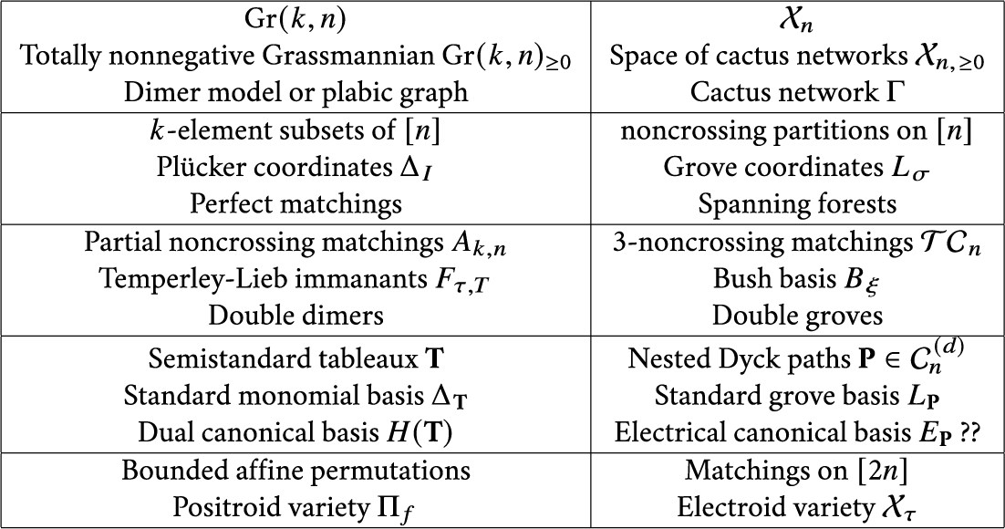
Figure 1: Parallels between
 $\mathcal {X}_n$
and
$\mathcal {X}_n$
and
 $\operatorname {\mathrm {Gr}}(k,n)$
.
$\operatorname {\mathrm {Gr}}(k,n)$
.
1.2 Plücker algebra and grove algebra
The Plücker algebra is the homogeneous coordinate ring
 $R(k,n):={\mathbb C}[\operatorname {\mathrm {Gr}}(k,n)]$
of the Grassmannian. It can be identified with the quotient of the polynomial ring
$R(k,n):={\mathbb C}[\operatorname {\mathrm {Gr}}(k,n)]$
of the Grassmannian. It can be identified with the quotient of the polynomial ring
 ${\mathbb C}[\Delta _I]$
generated by the Plücker coordinates
${\mathbb C}[\Delta _I]$
generated by the Plücker coordinates
 $\Delta _I$
, labeled by k-element subsets
$\Delta _I$
, labeled by k-element subsets
 $I \subset \binom {[n]}{k}$
, modulo the Plücker ideal generated by the Plücker relations. The Plücker algebra
$I \subset \binom {[n]}{k}$
, modulo the Plücker ideal generated by the Plücker relations. The Plücker algebra
 $R(k,n)$
is also isomorphic to the ring of
$R(k,n)$
is also isomorphic to the ring of
 $\operatorname {\mathrm {SL}}(k)$
-invariants in the polynomial functions on a
$\operatorname {\mathrm {SL}}(k)$
-invariants in the polynomial functions on a
 $k\times n$
matrix. In this latter setting, the description of
$k\times n$
matrix. In this latter setting, the description of
 $R(k,n)$
in terms of Plücker coordinates and Plücker relations are known as the first and second fundamental theorems of invariant theory.
$R(k,n)$
in terms of Plücker coordinates and Plücker relations are known as the first and second fundamental theorems of invariant theory.
We recall the following classical theorem regarding the basis for the Plücker ideal and the Plücker ring (see [Reference Sturmfels and WhiteSW89]).
Theorem 1.1
-
(1) The Plücker relations form a quadratic Gröbner basis for the Plücker ideal.
-
(2) The degree d homogeneous piece
 $R(k,n)_d$
of the Plücker ring has basis the set of standard monomials
$\Delta _{\mathbf {T}} = \Delta _{T_1}\Delta _{T_2} \cdots \Delta _{T_d}$
as
$(T_1,\ldots ,T_d)$
varies over the columns of a semistandard Young tableaux
${\mathbf {T}}$
with rectangular shape
$k \times d$
and entries in
$\{1,2,\ldots ,n\}$
.
$R(k,n)_d$
of the Plücker ring has basis the set of standard monomials
$\Delta _{\mathbf {T}} = \Delta _{T_1}\Delta _{T_2} \cdots \Delta _{T_d}$
as
$(T_1,\ldots ,T_d)$
varies over the columns of a semistandard Young tableaux
${\mathbf {T}}$
with rectangular shape
$k \times d$
and entries in
$\{1,2,\ldots ,n\}$
.


In analogy to the objects involved in Theorem 1.1, we define the grove algebra
 $G_{n}:={\mathbb C}[\mathcal {X}_n]$
to be homogeneous coordinate ring of
$G_{n}:={\mathbb C}[\mathcal {X}_n]$
to be homogeneous coordinate ring of
 $\mathcal {X}_n$
and use
$\mathcal {X}_n$
and use
 $G_{d,n}$
denote the degree d homogeneous piece of
$G_{d,n}$
denote the degree d homogeneous piece of
 $G_n$
. There is a natural bijection
$G_n$
. There is a natural bijection
 $P \mapsto \sigma (P)$
(see Section 2.4) from Dyck paths of semilength
$P \mapsto \sigma (P)$
(see Section 2.4) from Dyck paths of semilength
 $2n$
to noncrossing partitions of
$2n$
to noncrossing partitions of
 $[n]$
. We abuse notation by writing
$[n]$
. We abuse notation by writing
 $L_P$
for
$L_P$
for
 $L_{\sigma (P)}$
. Let
$L_{\sigma (P)}$
. Let
 $\mathcal {C}^{(d)}_n$
denote the set of d-tuples of nested Dyck paths (see Section 2.4). For
$\mathcal {C}^{(d)}_n$
denote the set of d-tuples of nested Dyck paths (see Section 2.4). For
 ${\mathbf {P}} = (P_1,\ldots ,P_d) \in \mathcal {C}^{(d)}_n$
, we define the standard grove monomials
${\mathbf {P}} = (P_1,\ldots ,P_d) \in \mathcal {C}^{(d)}_n$
, we define the standard grove monomials
 $$ \begin{align*}L_{\mathbf{P}}:= L_{P_1}L_{P_2} \dots L_{P_d}. \end{align*} $$
In this work, we present a result analogous to Theorem 1.1 for the grove algebra, stated as follows.
Theorem 1.2 (Theorem 6.11 and Proposition 6.4)
-
(1) The grove algebra
$G_n$
is generated by the grove coordinates
$L_\sigma $
modulo the ideal
$\mathfrak {I}_n$
generated by the quadratic relations
$r_{P,Q}$
described in Definition 6.2. The relations
$r_{P,Q}$
give a Gröbner basis of the ideal
$\mathfrak {I}_n$
, with respect to a term order described in Section 6. -
(2) We have
$\dim (G_{d,n}) = \prod _{1 \leq i \leq j \leq n-1} \frac {i+j+2d}{i+j}$
and
$G_{d,n}$
has basis the set of standard grove monomials
$L_{\mathbf {P}}$
,
${\mathbf {P}} \in \mathcal {C}^{(d)}_n$
.


Chepuri, George, and Speyer [Reference Chepuri, George and SpeyerCGS21] and Bychkov, Gorbounov, Kazakov, and Talalaev [Reference Bychkov, Gorbounov, Kazakov and TalalaevBGKT21] have shown that the variety
 $\mathcal {X}_n$
is isomorphic to the Lagrangian Grassmannian
$\mathcal {X}_n$
is isomorphic to the Lagrangian Grassmannian
 $\operatorname {\mathrm {LG}}(n-1,2n-2)$
, extending earlier work of Lam and Pylyavskyy [Reference Lam and PylyavskyyLP15] relating electrical networks to the symplectic group. By Borel–Weil theory, each homogeneous piece
$\operatorname {\mathrm {LG}}(n-1,2n-2)$
, extending earlier work of Lam and Pylyavskyy [Reference Lam and PylyavskyyLP15] relating electrical networks to the symplectic group. By Borel–Weil theory, each homogeneous piece
 $G_{d,n}$
of
$G_{d,n}$
of
 $G_n$
is isomorphic to an irreducible representation of the symplectic group
$G_n$
is isomorphic to an irreducible representation of the symplectic group
 $\operatorname {\mathrm {Sp}}(2n-2)$
(see Section 6.2). The relation between our description of
$\operatorname {\mathrm {Sp}}(2n-2)$
(see Section 6.2). The relation between our description of
 $G_{d,n}$
, including the standard grove basis
$G_{d,n}$
, including the standard grove basis
 $\{L_{\mathbf {P}}\}$
, and the usual constructions from highest weight theory of
$\{L_{\mathbf {P}}\}$
, and the usual constructions from highest weight theory of
 $\operatorname {\mathrm {Sp}}(2n-2)$
is far from being clear. It is an interesting problem to compare these approaches.
$\operatorname {\mathrm {Sp}}(2n-2)$
is far from being clear. It is an interesting problem to compare these approaches.
1.3 Electrical canonical basis
Recall that the standard monomial basis
 $\Delta _{{\mathbf {T}}}$
is not compatible with the cyclic symmetry of
$\Delta _{{\mathbf {T}}}$
is not compatible with the cyclic symmetry of
 $\operatorname {\mathrm {Gr}}(k,n)$
. Lusztig’s dual canonical basis of
$\operatorname {\mathrm {Gr}}(k,n)$
. Lusztig’s dual canonical basis of
 $R(k,n)$
is compatible with cyclic symmetry and exhibits remarkable positivity properties. See [Reference LamLam19] for the following result.
$R(k,n)$
is compatible with cyclic symmetry and exhibits remarkable positivity properties. See [Reference LamLam19] for the following result.
Theorem 1.3 The space
 $R(k,n)_d$
has a dual canonical basis
$R(k,n)_d$
has a dual canonical basis
 $H({\mathbf {T}})$
with the following properties:
$H({\mathbf {T}})$
with the following properties:
-
(1) For
$d=1$
, we have
$H({\mathbf {T}})= \Delta _I$
, where I is the set of entries in the one-column tableau
${\mathbf {T}}$
. -
(2) For
$d=2$
, the set
$\{H({\mathbf {T}})\}$
is exactly the set of Temperley–Lieb immanants [Reference LamLam15]
$\{F_{\tau ,T} \mid (\tau , T)\in A_{k,n}\}$
which we describe in Section 5. -
(3) For any semistandard tableau
${\mathbf {T}}$
, the function
$H({\mathbf {T}})$
is a nonnegative function on the totally nonnegative Grassmannian
$\operatorname {\mathrm {Gr}}(k,n)_{\geq 0}$
. -
(4) For any
${\mathbf {T}}$
, we have
$\chi ^*(H({\mathbf {T}})) = H(\chi ({\mathbf {T}}))$
where
$\chi ^*$
denotes the pullback map induced by the signed cyclic symmetry
$\chi :\operatorname {\mathrm {Gr}}(k, n)\to \operatorname {\mathrm {Gr}}(k, n)$
, and
$\chi ({\mathbf {T}})$
is the promotion of
${\mathbf {T}}$
.


In [Reference LamLam19] (see also [Reference LamLam16]), it is further shown that the dual canonical basis
 $H({\mathbf {T}})$
is compatible with restrictions to the homogeneous coordinate ring of positroid varieties
$H({\mathbf {T}})$
is compatible with restrictions to the homogeneous coordinate ring of positroid varieties
 $\Pi _f$
[Reference Knutson, Lam and SpeyerKLS13].
$\Pi _f$
[Reference Knutson, Lam and SpeyerKLS13].
Similar to the standard monomial basis for
 $\operatorname {\mathrm {Gr}}(k,n)$
, the standard grove basis
$\operatorname {\mathrm {Gr}}(k,n)$
, the standard grove basis
 $L_{\mathbf {P}}$
is not compatible with the cyclic symmetry of planar electrical networks (or that of
$L_{\mathbf {P}}$
is not compatible with the cyclic symmetry of planar electrical networks (or that of
 $\mathcal {X}_n$
). Therefore, we conjecture that there exists a canonical basis for the space
$\mathcal {X}_n$
). Therefore, we conjecture that there exists a canonical basis for the space
 $G_{d,n}$
analogous to the dual canonical basis
$G_{d,n}$
analogous to the dual canonical basis
 $H({\mathbf {T}})$
for
$H({\mathbf {T}})$
for
 $R(k_n)_d$
in Theorem 1.3.
$R(k_n)_d$
in Theorem 1.3.
Conjecture 1.4 The space
 $G_{d,n}$
has an electrical canonical basis
$G_{d,n}$
has an electrical canonical basis
 $E_{\mathbf {P}}$
,
$E_{\mathbf {P}}$
,
 ${\mathbf {P}} \in \mathcal {C}^{(d)}_n$
with the following properties:
${\mathbf {P}} \in \mathcal {C}^{(d)}_n$
with the following properties:
-
(1) For
$d = 1$
, we have
$E_P = L_P$
. -
(2) The electrical canonical basis takes nonnegative values on the compactification of the space of electrical networks
$\mathcal {X}_{n,\geq 0}$
. -
(3) Any monomial in the grove coordinates
$L_\sigma $
expands positively into the electrical canonical basis
$E_P$
. -
(4) There are actions of the cyclic group
$\mathbb {Z}/2n\mathbb {Z} = \langle \chi \rangle $
on
$\mathcal {C}^{(d)}_n$
and on
$\mathcal {X}_n$
, preserving
$\mathcal {X}_{n,\geq 0}$
, such that
$\chi ^*(E_{\mathbf {P}}) = E_{\chi ({\mathbf {P}})}$
, where
$\chi ^*$
denotes the pullback on
$\mathcal {X}_n$
induced by
$\chi $
.Footnote
1


The action of
 $\chi $
on
$\chi $
on
 $\mathcal {C}^{(d)}_n$
is an electrical analog of promotion on tableaux. For
$\mathcal {C}^{(d)}_n$
is an electrical analog of promotion on tableaux. For
 $d=1$
, it corresponds to rotation on noncrossing matchings, under the bijection between Dyck paths and noncrossing matchings (Section 2.4).
$d=1$
, it corresponds to rotation on noncrossing matchings, under the bijection between Dyck paths and noncrossing matchings (Section 2.4).
Lusztig has defined a totally nonnegative part
 $\operatorname {\mathrm {LG}}(n-1,2n-2)_{\geq 0}$
of
$\operatorname {\mathrm {LG}}(n-1,2n-2)_{\geq 0}$
of
 $\operatorname {\mathrm {LG}}(n-1, 2n-2)$
(see [Reference KarpmanKar18]). The spaces
$\operatorname {\mathrm {LG}}(n-1, 2n-2)$
(see [Reference KarpmanKar18]). The spaces
 $\mathcal {X}_{n,\geq 0}$
and
$\mathcal {X}_{n,\geq 0}$
and
 $\operatorname {\mathrm {LG}}(n-1,2n-2)_{\geq 0}$
are both “totally positive” versions of the Lagrangian Grassmannian. However, they are quite different. For example, they are cell complexes with a different number of cells. We expect the analogy between
$\operatorname {\mathrm {LG}}(n-1,2n-2)_{\geq 0}$
are both “totally positive” versions of the Lagrangian Grassmannian. However, they are quite different. For example, they are cell complexes with a different number of cells. We expect the analogy between
 $\operatorname {\mathrm {LG}}(n-1,2n-2)_{\geq 0}$
and
$\operatorname {\mathrm {LG}}(n-1,2n-2)_{\geq 0}$
and
 $\mathcal {X}_{n,\geq 0}$
to parallel the analogy between Lusztig’s dual canonical basis and the electrical canonical basis.
$\mathcal {X}_{n,\geq 0}$
to parallel the analogy between Lusztig’s dual canonical basis and the electrical canonical basis.
In [Reference LamLam18], a stratification of
 $\mathcal {X}_n$
by electroid varieties
$\mathcal {X}_n$
by electroid varieties
 $\mathcal {X}_\tau $
is constructed, indexed by matchings
$\mathcal {X}_\tau $
is constructed, indexed by matchings
 $\tau $
on
$\tau $
on
 $2n$
points. We conjecture the electrical canonical basis to have the following properties with respect to
$2n$
points. We conjecture the electrical canonical basis to have the following properties with respect to
 $\mathcal {X}_\tau $
.
$\mathcal {X}_\tau $
.
Conjecture 1.5
-
(1) For a matching
$\tau $
, the electrical canonical basis elements
$E_{\mathbf {P}}$
that do not restrict to 0 on
$\mathcal {X}_\tau $
form a basis of the homogeneous coordinate ring
${\mathbb C}[\mathcal {X}_\tau ]$
. -
(2) For a matching
$\tau $
, if
$E_{\mathbf {P}}$
is not identically 0 on
$\mathcal {X}_\tau $
, then it takes strictly positive values on
$\mathcal {X}_{\tau ,>0} = \mathcal {X}_\tau \cap \mathcal {X}_{n,\geq 0}$
.


1.4 Electrical canonical basis in degree two
Using the combinatorics of electrical networks, we construct the electrical canonical basis in degree two, which we call the Bush basis. As a consequence, we discover some remarkable combinatorial properties of double groves.
There is a bijection between the set
 $\mathcal {C}^{(2)}_n$
of pairs of nested Dyck paths of semilength
$\mathcal {C}^{(2)}_n$
of pairs of nested Dyck paths of semilength
 $2n$
, and the set of
$2n$
, and the set of
 $3$
-noncrossing matchings on
$3$
-noncrossing matchings on
 $2n$
points, defined in Section 3. We construct the Bush basis
$2n$
points, defined in Section 3. We construct the Bush basis
 $B_\xi $
of
$B_\xi $
of
 $G_{2,n}$
labeled by
$G_{2,n}$
labeled by
 $3$
-noncrossing matchings
$3$
-noncrossing matchings
 $\xi $
, defined by (Definition 4.3)
$\xi $
, defined by (Definition 4.3)
 $$ \begin{align*}B_\xi(\Gamma):= \sum_{H \subset 2\Gamma} \alpha(H)_\xi \operatorname{\mathrm{wt}}(H), \end{align*} $$
where the summation is over double groves in
 $\Gamma $
, and
$\Gamma $
, and
 $\alpha (H)_\xi $
are certain nonnegative integers. This definition is compatible with the natural rotation action on 3-noncrossing matchings. In Theorem 4.4, we give a positive expansion of the quadratic monomials
$\alpha (H)_\xi $
are certain nonnegative integers. This definition is compatible with the natural rotation action on 3-noncrossing matchings. In Theorem 4.4, we give a positive expansion of the quadratic monomials
 $L_\sigma L_{\sigma '}$
into the Bush basis
$L_\sigma L_{\sigma '}$
into the Bush basis
 $B_\xi $
.
$B_\xi $
.
The relation between
 $L_\sigma $
and
$L_\sigma $
and
 $\Delta _I$
is more than an analogy. In [Reference LamLam18], it is shown that the embedding
$\Delta _I$
is more than an analogy. In [Reference LamLam18], it is shown that the embedding
 $\iota :\mathcal {X}_n \hookrightarrow \operatorname {\mathrm {Gr}}(n-1,2n)$
is given by the formula
$\iota :\mathcal {X}_n \hookrightarrow \operatorname {\mathrm {Gr}}(n-1,2n)$
is given by the formula
 $$ \begin{align*}\iota^*(\Delta_I) = \sum_I M_{I\sigma} L_\sigma, \end{align*} $$
where
 $M_{I \sigma }$
is the concordance matrix defined in [Reference LamLam18] which we recall in Section 6.1. Likewise, we give in Section 5, a positive formula expanding the Temperley–Lieb immanants
$M_{I \sigma }$
is the concordance matrix defined in [Reference LamLam18] which we recall in Section 6.1. Likewise, we give in Section 5, a positive formula expanding the Temperley–Lieb immanants
 $F_{\tau ,T}$
in terms of the Bush basis
$F_{\tau ,T}$
in terms of the Bush basis
 $B_\xi $
. This produces a commutative square of positive expansions:
$B_\xi $
. This produces a commutative square of positive expansions:

It would also be interesting to carry out our program in the setting of the Ising model and orthogonal Grassmannian [Reference Galashin and PylyavskyyGP20].
2 Background
In this section, we introduce relevant background, following conventions in [Reference LamLam18].
2.1 Electrical networks and cactus networks
A circular planar electrical network, is a finite weighted undirected graph
 $\Gamma $
embedded into a disk, with boundary vertices labeled
$\Gamma $
embedded into a disk, with boundary vertices labeled
 $\bar 1,\bar 2,\ldots ,\bar n$
in clockwise order. From now on, we will simply refer to circular planar electrical networks as electrical networks.
$\bar 1,\bar 2,\ldots ,\bar n$
in clockwise order. From now on, we will simply refer to circular planar electrical networks as electrical networks.
Cactus networks are introduced by the second author [Reference LamLam18] in order to study the compactification of the space of electrical networks. Let S be a circle with boundary vertices
 $\bar 1,\ldots ,\bar n$
, and let
$\bar 1,\ldots ,\bar n$
, and let
 $\zeta $
be a noncrossing partition of
$\zeta $
be a noncrossing partition of
 $[\bar n]$
. Identifying the boundary vertices according to the parts of
$[\bar n]$
. Identifying the boundary vertices according to the parts of
 $\zeta $
gives a hollow cactus
$\zeta $
gives a hollow cactus
 $S_{\zeta }$
, which can be viewed as a union of circles glued at some points. A cactus is
$S_{\zeta }$
, which can be viewed as a union of circles glued at some points. A cactus is
 $S_{\zeta }$
together with its interior and a cactus network
$S_{\zeta }$
together with its interior and a cactus network
 $\Gamma $
is a weighted graph embedded into a cactus, which can be intuitively thought of as an electrical network where boundary vertices are identified in a manner given by
$\Gamma $
is a weighted graph embedded into a cactus, which can be intuitively thought of as an electrical network where boundary vertices are identified in a manner given by
 $\zeta $
. In particular, an electrical network is a cactus network with
$\zeta $
. In particular, an electrical network is a cactus network with
 $\zeta =(\bar 1|\bar 2|\cdots |\bar {n})$
. See Figure 2 for an example.
$\zeta =(\bar 1|\bar 2|\cdots |\bar {n})$
. See Figure 2 for an example.
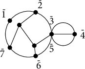
Figure 2: An example of a cactus network for
 $\zeta =(\bar 1|\bar 2|\bar 3,\bar 5|\bar 4|\bar 6|\bar 7)$
.
$\zeta =(\bar 1|\bar 2|\bar 3,\bar 5|\bar 4|\bar 6|\bar 7)$
.
We can define a weight function
 $\operatorname {\mathrm {wt}}$
on the edges in a network
$\operatorname {\mathrm {wt}}$
on the edges in a network
 $\Gamma $
, where we typically treat each value
$\Gamma $
, where we typically treat each value
 $\operatorname {\mathrm {wt}}(e)$
as an indeterminate. For a subgraph
$\operatorname {\mathrm {wt}}(e)$
as an indeterminate. For a subgraph
 $F\subset \Gamma $
, define
$F\subset \Gamma $
, define
 $$\begin{align*}\operatorname{\mathrm{wt}}(F)=\prod_{e\in F}\operatorname{\mathrm{wt}}(e).\end{align*}$$
We call the underlying unweighted graph of a cactus network a cactus graph.
2.2 Groves
A grove F on a cactus network
 $\Gamma $
is a spanning forest, such that each component is connected to the boundary. The boundary partition
$\Gamma $
is a spanning forest, such that each component is connected to the boundary. The boundary partition
 $\sigma (F)$
is a set partition of
$\sigma (F)$
is a set partition of
 $[\bar n]$
that records which boundary vertices are in the same connected components of F. Note that since our network is planar,
$[\bar n]$
that records which boundary vertices are in the same connected components of F. Note that since our network is planar,
 $\sigma (F)$
must be a noncrossing partition of
$\sigma (F)$
must be a noncrossing partition of
 $[\bar n]$
that coarsens
$[\bar n]$
that coarsens
 $\zeta $
, if
$\zeta $
, if
 $\Gamma $
lies in the cactus
$\Gamma $
lies in the cactus
 $S_{\zeta }$
. For a noncrossing partition
$S_{\zeta }$
. For a noncrossing partition
 $\sigma $
, we define the grove measurement as
$\sigma $
, we define the grove measurement as
 $$\begin{align*}L_{\sigma}(\Gamma):=\sum_{F\:|\: \sigma(F)=\sigma}\operatorname{\mathrm{wt}}(F),\end{align*}$$
where the summation is over all groves with boundary partition
 $\sigma $
.
$\sigma $
.
2.3 Medial graph and medial pairing
Given a cactus network
 $\Gamma $
, we define its medial graph
$\Gamma $
, we define its medial graph
 $G(\Gamma )$
as follows. The vertices of
$G(\Gamma )$
as follows. The vertices of
 $G(\Gamma )$
consist of vertices
$G(\Gamma )$
consist of vertices
 $t_1,t_2,\ldots ,t_{2n}$
on the boundary in clockwise order such that the original boundary vertex
$t_1,t_2,\ldots ,t_{2n}$
on the boundary in clockwise order such that the original boundary vertex
 $\bar i$
lies between
$\bar i$
lies between
 $t_{2i-1}$
and
$t_{2i-1}$
and
 $t_{2i}$
, and vertices
$t_{2i}$
, and vertices
 $t_e$
’s for each edge e in the network. The edges of
$t_e$
’s for each edge e in the network. The edges of
 $G(\Gamma )$
are joined as follows: we first join
$G(\Gamma )$
are joined as follows: we first join
 $t_e$
with
$t_e$
with
 $t_{e'}$
if e and
$t_{e'}$
if e and
 $e'$
share a vertex of
$e'$
share a vertex of
 $\Gamma $
and are incident to the same face. Then for each boundary vertex
$\Gamma $
and are incident to the same face. Then for each boundary vertex
 $\bar i$
of
$\bar i$
of
 $\Gamma $
, let the edges incident to
$\Gamma $
, let the edges incident to
 $\bar i$
be
$\bar i$
be
 $e_1,\ldots ,e_k$
in counterclockwise order, i.e.,
$e_1,\ldots ,e_k$
in counterclockwise order, i.e.,
 $t_{2i-1}$
is closest to
$t_{2i-1}$
is closest to
 $e_1$
while
$e_1$
while
 $t_{2i}$
is closest to
$t_{2i}$
is closest to
 $e_{k}$
, and join
$e_{k}$
, and join
 $t_{2i-1}$
with
$t_{2i-1}$
with
 $t_{e_1}$
and
$t_{e_1}$
and
 $t_{2i}$
with
$t_{2i}$
with
 $t_{e_k}$
; in the case of
$t_{e_k}$
; in the case of
 $k=0$
, i.e., there are no edges incident to
$k=0$
, i.e., there are no edges incident to
 $\bar i$
in
$\bar i$
in
 $\Gamma $
, we join
$\Gamma $
, we join
 $t_{2i-1}$
with
$t_{2i-1}$
with
 $t_{2i}$
instead. Note that in
$t_{2i}$
instead. Note that in
 $G(\Gamma )$
, each
$G(\Gamma )$
, each
 $t_e$
has degree
$t_e$
has degree
 $4$
for
$4$
for
 $e\in E(\Gamma )$
, and each
$e\in E(\Gamma )$
, and each
 $t_i$
has degree
$t_i$
has degree
 $1$
for
$1$
for
 $i\in [2n]$
.
$i\in [2n]$
.
We then define the medial pairing
 $\tau (\Gamma )$
on a medial graph
$\tau (\Gamma )$
on a medial graph
 $G(\Gamma )$
. From a boundary vertex
$G(\Gamma )$
. From a boundary vertex
 $t_i$
, which has degree
$t_i$
, which has degree
 $1$
of
$1$
of
 $G(\Gamma )$
, we trace through edges such that whenever we encounter a degree
$G(\Gamma )$
, we trace through edges such that whenever we encounter a degree
 $4$
vertex
$4$
vertex
 $t_e$
, we go straight through, ending at another boundary vertex
$t_e$
, we go straight through, ending at another boundary vertex
 $t_j$
. This procedure forms n strands or wires which naturally results in a matching
$t_j$
. This procedure forms n strands or wires which naturally results in a matching
 $\tau (\Gamma )$
of
$\tau (\Gamma )$
of
 $[2n]$
. See Figure 3 for an example.
$[2n]$
. See Figure 3 for an example.
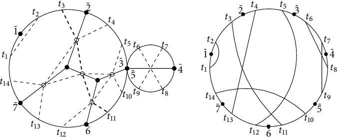
Figure 3: A cactus network
 $\Gamma $
with its medial graph
$\Gamma $
with its medial graph
 $G(\Gamma )$
(left) and medial pairing
$G(\Gamma )$
(left) and medial pairing
 $\tau (\Gamma )=\{(1,2),(3,11),(4,13),(5,12),(6,8),(7,9),(10,14)\}$
(right).
$\tau (\Gamma )=\{(1,2),(3,11),(4,13),(5,12),(6,8),(7,9),(10,14)\}$
(right).
For later sections, it might be more convenient to think about medial graphs and medial pairings to be on a circle instead of on a cactus. To reconstruct
 $\Gamma $
from its medial graph
$\Gamma $
from its medial graph
 $G(\Gamma )$
, either drawn on a cactus or drawn on a circle, we first place a boundary vertex
$G(\Gamma )$
, either drawn on a cactus or drawn on a circle, we first place a boundary vertex
 $\bar i$
between
$\bar i$
between
 $t_{2i-1}$
and
$t_{2i-1}$
and
 $t_{2i}$
for
$t_{2i}$
for
 $i\in [n]$
. Note that the graph G divides the interior of the disk or the cactus into regions. We color the regions with black and white so that adjacent regions have different colors, and that the regions with boundary vertices
$i\in [n]$
. Note that the graph G divides the interior of the disk or the cactus into regions. We color the regions with black and white so that adjacent regions have different colors, and that the regions with boundary vertices
 $\bar i$
’s are colored white. Contract the boundary vertices inside the same regions to form a cactus. Place a vertex in each white interior region and connect two vertices if the two corresponding regions in G share a vertex.
$\bar i$
’s are colored white. Contract the boundary vertices inside the same regions to form a cactus. Place a vertex in each white interior region and connect two vertices if the two corresponding regions in G share a vertex.
A medial graph is lensless if no wire has a self intersection, and no two wires cross twice, i.e., there are no lens that look like ![]() . A cactus network
. A cactus network
 $\Gamma $
is critical, or reduced, if its medial graph is lensless. In this case, the number of crossings in the medial pairing
$\Gamma $
is critical, or reduced, if its medial graph is lensless. In this case, the number of crossings in the medial pairing
 $\tau (\Gamma )$
equals the number of edges in
$\tau (\Gamma )$
equals the number of edges in
 $\Gamma $
. We note that for any matching
$\Gamma $
. We note that for any matching
 $\tau $
on
$\tau $
on
 $[2n]$
, there exists a reduced cactus network
$[2n]$
, there exists a reduced cactus network
 $\Gamma $
such that
$\Gamma $
such that
 $\tau (\Gamma )=\tau $
, by drawing
$\tau (\Gamma )=\tau $
, by drawing
 $\tau $
in a reduced way on a disk, viewing it as a medial graph and applying the procedure above. More specifically, we recall the following Proposition 2.1 from [Reference LamLam18].
$\tau $
in a reduced way on a disk, viewing it as a medial graph and applying the procedure above. More specifically, we recall the following Proposition 2.1 from [Reference LamLam18].
Proposition 2.1 (Proposition 2.12 of [Reference LamLam18])
We have:
-
(1) any matching on
$[2n]$
can be realized as a medial pairing of some reduced cactus graph; -
(2) any two reduced cactus graphs with the same medial pairing can be obtained from each other via
$Y-\Delta $
moves.


Given a cactus network
 $\Gamma $
with its medial graph
$\Gamma $
with its medial graph
 $G(\Gamma )$
, we define its dual network
$G(\Gamma )$
, we define its dual network
 $\Gamma ^\vee $
as follows: we keep only the information of
$\Gamma ^\vee $
as follows: we keep only the information of
 $G(\Gamma )$
, put
$G(\Gamma )$
, put
 $\bar i$
between
$\bar i$
between
 $t_{2i}$
and
$t_{2i}$
and
 $t_{2i+1}$
in clockwise order where the indices are taken modulo
$t_{2i+1}$
in clockwise order where the indices are taken modulo
 $2n$
, and recover a cactus network
$2n$
, and recover a cactus network
 $\Gamma ^{\vee }$
via the procedure described above, called the dual network of
$\Gamma ^{\vee }$
via the procedure described above, called the dual network of
 $\Gamma $
. See Figure 4 for an example. If we take the dual twice,
$\Gamma $
. See Figure 4 for an example. If we take the dual twice,
 $(\Gamma ^{\vee })^{\vee }$
will be
$(\Gamma ^{\vee })^{\vee }$
will be
 $\Gamma $
with indices shifted by
$\Gamma $
with indices shifted by
 $1$
in the clockwise order.
$1$
in the clockwise order.

Figure 4: A network
 $\Gamma $
and its dual
$\Gamma $
and its dual
 $\Gamma ^{\vee }$
.
$\Gamma ^{\vee }$
.
The dual graphs
 $\Gamma $
and
$\Gamma $
and
 $\Gamma ^{\vee }$
have the same number of edges. Furthermore, each edge of
$\Gamma ^{\vee }$
have the same number of edges. Furthermore, each edge of
 $\Gamma $
intersects a unique edge of
$\Gamma $
intersects a unique edge of
 $\Gamma ^\vee $
(and vice-versa), inducing a natural bijection between the edges of
$\Gamma ^\vee $
(and vice-versa), inducing a natural bijection between the edges of
 $\Gamma $
and of
$\Gamma $
and of
 $\Gamma ^\vee $
. Each pair of intersecting edges corresponds to an intersection in the medial graph
$\Gamma ^\vee $
. Each pair of intersecting edges corresponds to an intersection in the medial graph
 $G(\Gamma )$
.
$G(\Gamma )$
.
2.4 Catalan objects and their bijections
We need to use all of the following objects: Dyck paths, noncrossing matchings and noncrossing partitions, all of which are enumerated by the Catalan numbers
 $C_n$
. For easier reference, we summarize the notations we use in the following:
$C_n$
. For easier reference, we summarize the notations we use in the following:
-
-
$\mathcal {C}_n$
:= the set of Dyck paths of semilength n. -
-
$\mathcal {M}_n$
:= the set of matchings on
$1,2,\ldots ,2n$
. -
-
$\mathcal {NM}_n$
:= the set of noncrossing matchings on
$1,2,\ldots ,2n$
. -
-
$\mathcal {TC}_n$
:= the set of
$3$
-noncrossing matchings on
$1,2,\ldots ,2n$
. -
-
$\mathcal {NP}_n$
:= the set of noncrossing partitions of
$[\bar {n}] = \{\bar {1}, \bar {2},\dots , \bar {n}\}$
.


Now we start our discussion on these Catalan objects.
Definition 2.1 A Dyck path of semilength n is a walk from
 $(0,0)$
to
$(0,0)$
to
 $(2n,0)$
consisting of n upsteps
$(2n,0)$
consisting of n upsteps
 $(1,1)$
and n downsteps
$(1,1)$
and n downsteps
 $(1,-1)$
that stays above the x-axis.
$(1,-1)$
that stays above the x-axis.
We denote the set of Dyck paths of semilength n by
 $\mathcal {C}_n$
. There is a natural poset structure on Dyck paths: for two Dyck paths of semilength n, we say that
$\mathcal {C}_n$
. There is a natural poset structure on Dyck paths: for two Dyck paths of semilength n, we say that
 $P\leq Q$
if the path P stays weakly below Q. We can also represent a Dyck path P by a vector
$P\leq Q$
if the path P stays weakly below Q. We can also represent a Dyck path P by a vector
 $v(P)\in \{0,1\}^{2n}$
such that
$v(P)\in \{0,1\}^{2n}$
such that
 $v(P)_j=1$
if the jth step of P is an upstep and
$v(P)_j=1$
if the jth step of P is an upstep and
 $v(P)_j=0$
if the jth step of P is a downstep. Then there are always as many
$v(P)_j=0$
if the jth step of P is a downstep. Then there are always as many
 $1$
’s as
$1$
’s as
 $0$
’s within
$0$
’s within
 $v(P)_1,\ldots ,v(P)_j$
for all
$v(P)_1,\ldots ,v(P)_j$
for all
 $j=1,\ldots ,2n$
. We write
$j=1,\ldots ,2n$
. We write
 $P\preccurlyeq Q$
if
$P\preccurlyeq Q$
if
 $v(P)$
is lexicographically (weakly) smaller than
$v(P)$
is lexicographically (weakly) smaller than
 $v(Q)$
. Note that
$v(Q)$
. Note that
 $\preccurlyeq $
is a total order and that if
$\preccurlyeq $
is a total order and that if
 $P\leq Q$
then
$P\leq Q$
then
 $P\preccurlyeq Q$
.
$P\preccurlyeq Q$
.
For a positive integer k, let
 $$\begin{align*}\mathcal{C}_n^{(k)}=\{P_1\leq P_2\leq\cdots\leq P_k\}\subset \mathcal{C}_n^{k}\end{align*}$$
be the set of chains of length k in the poset on Dyck paths of semilength n. In particular,
 $\mathcal {C}_n^{(1)}=\mathcal {C}_n$
and
$\mathcal {C}_n^{(1)}=\mathcal {C}_n$
and
 $\mathcal {C}_n^{(2)}$
is the set of pairs of comparable Dyck paths
$\mathcal {C}_n^{(2)}$
is the set of pairs of comparable Dyck paths
 $(P\leq Q)$
.
$(P\leq Q)$
.
Another important family of combinatorial objects that we need is matchings. Denote the set of matchings on
 $1,2,\ldots ,2n$
by
$1,2,\ldots ,2n$
by
 $\mathcal {M}_n$
. For a pair
$\mathcal {M}_n$
. For a pair
 $(i,j)$
in a matching M with
$(i,j)$
in a matching M with
 $i<j$
, we say that i is the left endpoint and j is the right endpoint. Let
$i<j$
, we say that i is the left endpoint and j is the right endpoint. Let
 $\mathrm {cr}(M)$
denote the set of crossings of M, given by
$\mathrm {cr}(M)$
denote the set of crossings of M, given by
 $$\begin{align*}\mathrm{cr}(M)=\{(a,b,c,d)\:|\: a<b<c<d,\ (a,c),(b,d)\in M\}.\end{align*}$$
A strand diagram of a matching
 $M\in \mathcal {M}_n$
is a drawing of M by n arcs, called strands or wires, either on a disk or a straight line such that no two strands cross twice. We consider the strand diagrams up to homotopy so for example, if
$M\in \mathcal {M}_n$
is a drawing of M by n arcs, called strands or wires, either on a disk or a straight line such that no two strands cross twice. We consider the strand diagrams up to homotopy so for example, if
 $M=\{(1,2),(3,4),\ldots ,(2n-1,2n)\}$
, then there is a unique strand diagram of M.
$M=\{(1,2),(3,4),\ldots ,(2n-1,2n)\}$
, then there is a unique strand diagram of M.
Definition 2.2 A matching M of
 $1,2,\ldots ,2n$
is called k-noncrossing if there do not exist k pairs in M that cross pairwise. Denote the set of
$1,2,\ldots ,2n$
is called k-noncrossing if there do not exist k pairs in M that cross pairwise. Denote the set of
 $2$
-noncrossing matchings, i.e., noncrossing matchings by
$2$
-noncrossing matchings, i.e., noncrossing matchings by
 $\mathcal {NM}_n$
and the set of
$\mathcal {NM}_n$
and the set of
 $3$
-noncrossing matchings by
$3$
-noncrossing matchings by
 $\mathcal {TC}_n$
.
$\mathcal {TC}_n$
.
We now describe a bijection between Dyck paths
 $\mathcal {C}_n$
and noncrossing matchings
$\mathcal {C}_n$
and noncrossing matchings
 $\mathcal {NM}_n$
. For a Dyck path
$\mathcal {NM}_n$
. For a Dyck path
 $P\in \mathcal {C}_n$
, label its steps (edges) by
$P\in \mathcal {C}_n$
, label its steps (edges) by
 $1,2,\ldots ,2n$
from left to right and pair up the upsteps with downsteps of the same height with no steps in between to obtain a noncrossing matching
$1,2,\ldots ,2n$
from left to right and pair up the upsteps with downsteps of the same height with no steps in between to obtain a noncrossing matching
 $M\in \mathcal {NM}_n$
. For the inverse, given a noncrossing matching M, construct a Dyck path P so that the ith step is a upstep if i is a left endpoint in M, and a downstep if i is a right endpoint in M. See Figure 5 for an example.
$M\in \mathcal {NM}_n$
. For the inverse, given a noncrossing matching M, construct a Dyck path P so that the ith step is a upstep if i is a left endpoint in M, and a downstep if i is a right endpoint in M. See Figure 5 for an example.
Figure 5: Example of a Dyck path of semilength 5 and its corresponding noncrossing matching under the bijection described above.
Th cover relations in the poset structure on Dyck paths can be described as follows:
 $P\lessdot P'$
if
$P\lessdot P'$
if
 $P'$
can be obtained from P by changing an upstep followed by a downstep, to a downstep followed by an upstep. The poset structure on noncrossing matchings is inherited from that on Dyck paths. And the cover relations can be described similarly:
$P'$
can be obtained from P by changing an upstep followed by a downstep, to a downstep followed by an upstep. The poset structure on noncrossing matchings is inherited from that on Dyck paths. And the cover relations can be described similarly:
 $M\lessdot M'$
if we can change two pairs
$M\lessdot M'$
if we can change two pairs
 $(a,b)$
and
$(a,b)$
and
 $(b+1,c)$
in M to
$(b+1,c)$
in M to
 $(a,c)$
and
$(a,c)$
and
 $(b,b+1)$
in
$(b,b+1)$
in
 $M'$
, where
$M'$
, where
 $a<b<b+1<c$
.
$a<b<b+1<c$
.
Our third Catalan object is the set of noncrossing partitions.
Definition 2.3 A partition
 $\sigma $
of
$\sigma $
of
 $[\bar n]=\{\bar 1,\bar 2,\ldots ,\bar n\}$
is called noncrossing if there do not exist
$[\bar n]=\{\bar 1,\bar 2,\ldots ,\bar n\}$
is called noncrossing if there do not exist
 $a<b<c<d$
such that
$a<b<c<d$
such that
 $\bar a$
and
$\bar a$
and
 $\bar c$
are in one part of
$\bar c$
are in one part of
 $\sigma $
while
$\sigma $
while
 $\bar b$
and
$\bar b$
and
 $\bar d$
are in another. Denote the set of noncrossing partitions as
$\bar d$
are in another. Denote the set of noncrossing partitions as
 $\mathcal {NP}_n$
.
$\mathcal {NP}_n$
.
The natural bijections between
 $\mathcal {NP}_n$
and
$\mathcal {NP}_n$
and
 $\mathcal {NM}_n$
and
$\mathcal {NM}_n$
and
 $\mathcal {C}_n$
are also easy to describe.
$\mathcal {C}_n$
are also easy to describe.
We first start by describing the bijection between
 $\mathcal {NM}_n$
and
$\mathcal {NM}_n$
and
 $\mathcal {NP}_n$
. Let
$\mathcal {NP}_n$
. Let
 $M\in \mathcal {NM}_n$
be a noncrossing matching on
$M\in \mathcal {NM}_n$
be a noncrossing matching on
 $[2n]$
. We draw the strand diagram M either on a circle or on a straight line, dividing into smaller regions, put
$[2n]$
. We draw the strand diagram M either on a circle or on a straight line, dividing into smaller regions, put
 $\bar i$
between
$\bar i$
between
 $2i-1$
and
$2i-1$
and
 $2i$
, for
$2i$
, for
 $i=1,\ldots ,n$
. We obtain a noncrossing partition
$i=1,\ldots ,n$
. We obtain a noncrossing partition
 $\sigma $
of
$\sigma $
of
 $[\bar n]$
whose parts consist of the points
$[\bar n]$
whose parts consist of the points
 $\bar i$
in the same region. The inverse bijection from
$\bar i$
in the same region. The inverse bijection from
 $\mathcal {NP}_n$
to
$\mathcal {NP}_n$
to
 $\mathcal {NM}_n$
is more conveniently described inductively. Let
$\mathcal {NM}_n$
is more conveniently described inductively. Let
 $\sigma $
be a noncrossing partition, then
$\sigma $
be a noncrossing partition, then
 $\sigma $
must contain a part of the form
$\sigma $
must contain a part of the form
 $(a+1,\ldots ,a+k)$
for some
$(a+1,\ldots ,a+k)$
for some
 $a\geq 0$
and
$a\geq 0$
and
 $k\geq 1$
. We remove this part and add a partial matching by connecting
$k\geq 1$
. We remove this part and add a partial matching by connecting
 $2a+1$
with
$2a+1$
with
 $2a+2k$
,
$2a+2k$
,
 $2a+2$
with
$2a+2$
with
 $2a+3$
,
$2a+3$
,
 $2a+4$
with
$2a+4$
with
 $2a+5$
and so on up to
$2a+5$
and so on up to
 $2a+2k-2$
with
$2a+2k-2$
with
 $2a+2k-1$
. We repeat this process until we obtain a noncrossing matching.
$2a+2k-1$
. We repeat this process until we obtain a noncrossing matching.
Now we describe the bijection between
 $\mathcal {C}_n$
and
$\mathcal {C}_n$
and
 $\mathcal {NP}_n$
. Let
$\mathcal {NP}_n$
. Let
 $P\in \mathcal {C}_n$
be a Dyck path. There are
$P\in \mathcal {C}_n$
be a Dyck path. There are
 $2n+1$
lattice points in P, including
$2n+1$
lattice points in P, including
 $(0,0)$
and
$(0,0)$
and
 $(2n,0)$
. Label the
$(2n,0)$
. Label the
 $2i$
th lattice point in P by
$2i$
th lattice point in P by
 $\bar i$
, for
$\bar i$
, for
 $i=1,\ldots ,n$
, so that
$i=1,\ldots ,n$
, so that
 $(1,1)$
is labeled by
$(1,1)$
is labeled by
 $\bar 1$
. Then we identify
$\bar 1$
. Then we identify
 $\bar i$
and
$\bar i$
and
 $\bar j$
to be in the same part of the noncrossing partition
$\bar j$
to be in the same part of the noncrossing partition
 $\sigma $
if they are on the same horizontal line, not separated by the Dyck path P. To go the other way, we apply the following recursive procedure. Let
$\sigma $
if they are on the same horizontal line, not separated by the Dyck path P. To go the other way, we apply the following recursive procedure. Let
 $\sigma $
be a noncrossing partition and let the part containing
$\sigma $
be a noncrossing partition and let the part containing
 $1$
be
$1$
be
 $\{1=a_0<a_1<\cdots <a_k=m\}$
with
$\{1=a_0<a_1<\cdots <a_k=m\}$
with
 $k\geq 0$
. This means that each part of
$k\geq 0$
. This means that each part of
 $\sigma $
either has all entries at most m, or has all entries at least
$\sigma $
either has all entries at most m, or has all entries at least
 $m+1$
. We deal with these two kinds separately and attach the two resulting Dyck paths at coordinate
$m+1$
. We deal with these two kinds separately and attach the two resulting Dyck paths at coordinate
 $(2m,0)$
. Thus assume
$(2m,0)$
. Thus assume
 $m=n$
. Similarly, all other parts of
$m=n$
. Similarly, all other parts of
 $\sigma $
have their entries strictly between
$\sigma $
have their entries strictly between
 $a_i$
and
$a_i$
and
 $a_{i+1}$
, and let
$a_{i+1}$
, and let
 $P^{(i)}$
be the Dyck path obtained from such i, after adjusting the entries from
$P^{(i)}$
be the Dyck path obtained from such i, after adjusting the entries from
 $\{a_i+1,\ldots ,a_{i+1}-1\}$
to
$\{a_i+1,\ldots ,a_{i+1}-1\}$
to
 $\{1,\ldots ,a_{i+1}-a_i-1\}$
. Attach each
$\{1,\ldots ,a_{i+1}-a_i-1\}$
. Attach each
 $P^{(i)}$
from
$P^{(i)}$
from
 $(2a_i+2,2)$
to
$(2a_i+2,2)$
to
 $(2a_{i+1}-2,2)$
and we have the desired Dyck path
$(2a_{i+1}-2,2)$
and we have the desired Dyck path
 $P\in \mathcal {C}_n$
.
$P\in \mathcal {C}_n$
.
See Figure 6 for an illustration of the bijections between
 $\mathcal {NP}_n, \mathcal {NM}_n$
and
$\mathcal {NP}_n, \mathcal {NM}_n$
and
 $\mathcal {C}_n$
.
$\mathcal {C}_n$
.

Figure 6: The noncrossing matching (left) and the Dyck path (right) in bijection with the noncrossing partition
 $\sigma =(\bar 1\bar 2|\bar 3\bar 4\bar 5)$
.
$\sigma =(\bar 1\bar 2|\bar 3\bar 4\bar 5)$
.
For a noncrossing partition
 $\sigma $
on
$\sigma $
on
 $[\bar n]$
, one has a dual noncrossing partition
$[\bar n]$
, one has a dual noncrossing partition ![]() on
on ![]() obtained by drawing
obtained by drawing
 $\sigma $
on a disk, connecting boundary vertices in the same parts, putting
$\sigma $
on a disk, connecting boundary vertices in the same parts, putting ![]() between
between
 $\bar i$
and
$\bar i$
and
 $\overline {i{+}1}$
and identifying the partition
$\overline {i{+}1}$
and identifying the partition ![]() as the regions (see Figure 7). We also often denote
as the regions (see Figure 7). We also often denote
 $\sigma $
as a partition on
$\sigma $
as a partition on
 $1,3,\ldots ,2n-1$
and
$1,3,\ldots ,2n-1$
and ![]() as a partition on
as a partition on
 $2,4,\ldots ,2n$
.
$2,4,\ldots ,2n$
.
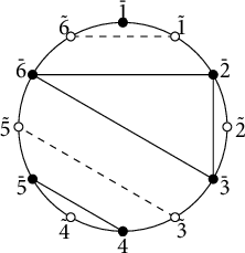
Figure 7: A noncrossing partition
 $\sigma =(\bar 1|\bar 2\bar 3\bar 6|\bar 4\bar 5)$
with its dual
$\sigma =(\bar 1|\bar 2\bar 3\bar 6|\bar 4\bar 5)$
with its dual ![]() .
.
It is easy to obtain that ![]() , where
, where
 $|\sigma |$
is the number of parts of
$|\sigma |$
is the number of parts of
 $\sigma $
(Lemma 2.2 of [Reference LamLam18]).
$\sigma $
(Lemma 2.2 of [Reference LamLam18]).
As for notations, we typically use
 $P,Q$
for Dyck paths,
$P,Q$
for Dyck paths,
 $\tau ,M,\xi $
for matchings, and
$\tau ,M,\xi $
for matchings, and
 $\sigma $
for noncrossing partitions. Also, denote these bijections by
$\sigma $
for noncrossing partitions. Also, denote these bijections by
 $\sigma :\mathcal {C}_n\rightarrow \mathcal {NP}_n$
,
$\sigma :\mathcal {C}_n\rightarrow \mathcal {NP}_n$
,
 $\sigma :\mathcal {NM}_n\rightarrow \mathcal {NP}_n$
,
$\sigma :\mathcal {NM}_n\rightarrow \mathcal {NP}_n$
,
 $\tau :\mathcal {C}_n\rightarrow \mathcal {NM}_n$
,
$\tau :\mathcal {C}_n\rightarrow \mathcal {NM}_n$
,
 $\tau :\mathcal {NP}_n\rightarrow \mathcal {NM}_n$
.
$\tau :\mathcal {NP}_n\rightarrow \mathcal {NM}_n$
.
3 Combinatorics of
$3$
-noncrossing matchings

3.1 3-noncrossing matchings and pairs of comparable Dyck paths
In this section, we describe a bijection between
 $3$
-noncrossing matchings
$3$
-noncrossing matchings
 $\mathcal {TC}_n$
of n and pairs of comparable Dyck paths
$\mathcal {TC}_n$
of n and pairs of comparable Dyck paths
 $\mathcal {C}_n^{(2)}$
in two languages, one formulated as in [Reference Chen, Deng, Du, Stanley and YanCDD+07] and the other one to be used later.
$\mathcal {C}_n^{(2)}$
in two languages, one formulated as in [Reference Chen, Deng, Du, Stanley and YanCDD+07] and the other one to be used later.
We first formulate the construction in Chen et al. [Reference Chen, Deng, Du, Stanley and YanCDD+07]. For a matching
 $M\in \mathcal {M}_n$
, associate a sequence of standard Young tableaux
$M\in \mathcal {M}_n$
, associate a sequence of standard Young tableaux
 $T_0,T_1,\ldots ,T_{2n}$
, starting with
$T_0,T_1,\ldots ,T_{2n}$
, starting with
 $T_{2n}=\emptyset $
, and for
$T_{2n}=\emptyset $
, and for
 $j<2n$
,
$j<2n$
,
-
• if j is the right end point of a pair
$(i,j)$
in M, insert i into
$T_{j+1}$
to obtain
$T_j$
, in the sense of row insertion in RSK (see, for example, [Reference StanleySta12]); -
• if j is the left end point of a pair
$(j,k)$
in M, delete j from
$T_{j+1}$
to obtain
$T_j$
.


For a k-noncrossing matching M,
 $k\geq 2$
, Chen et al. [Reference Chen, Deng, Du, Stanley and YanCDD+07] showed that the tableaux
$k\geq 2$
, Chen et al. [Reference Chen, Deng, Du, Stanley and YanCDD+07] showed that the tableaux
 $T_0,\ldots ,T_{2n}$
contain at most
$T_0,\ldots ,T_{2n}$
contain at most
 $k-1$
rows. Thus, for
$k-1$
rows. Thus, for
 $M\in \mathcal {TC}_n$
, let the shape of the corresponding standard Young tableau
$M\in \mathcal {TC}_n$
, let the shape of the corresponding standard Young tableau
 $T_{j}$
be
$T_{j}$
be
 $(x_j\geq y_j)$
. Note that the
$(x_j\geq y_j)$
. Note that the
 $y_j$
’s can be
$y_j$
’s can be
 $0$
. Define the map
$0$
. Define the map
 $\varphi : \mathcal {TC}_n\to \mathcal {C}_n^{(2)}$
as
$\varphi : \mathcal {TC}_n\to \mathcal {C}_n^{(2)}$
as
 $\varphi (M):=(P_1\leq P_2)$
, where
$\varphi (M):=(P_1\leq P_2)$
, where
 $P_1$
is the Dyck path that passes through the coordinates
$P_1$
is the Dyck path that passes through the coordinates
 $\{(j,x_j-y_j)\}_{j=0}^{2n}$
and
$\{(j,x_j-y_j)\}_{j=0}^{2n}$
and
 $P_2$
is the Dyck path that passes through the coordinates
$P_2$
is the Dyck path that passes through the coordinates
 $\{(j,x_j+y_j)\}_{j=0}^{2n}$
. See Figure 8 for an example.
$\{(j,x_j+y_j)\}_{j=0}^{2n}$
. See Figure 8 for an example.
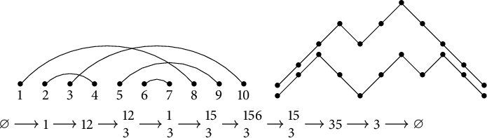
Figure 8: A bijection between
 $\mathcal {TC}_n$
and
$\mathcal {TC}_n$
and
 $\mathcal {C}^{(2)}_n$
by Chen et al. [Reference Chen, Deng, Du, Stanley and YanCDD+07], with the sequence of standard Young tableau
$\mathcal {C}^{(2)}_n$
by Chen et al. [Reference Chen, Deng, Du, Stanley and YanCDD+07], with the sequence of standard Young tableau
 $T_0,T_1,\ldots ,T_{2n}$
shown below.
$T_0,T_1,\ldots ,T_{2n}$
shown below.
Theorem 3.1 (Corollary 5.4 of [Reference Chen, Deng, Du, Stanley and YanCDD+07])
The map
 $\varphi $
defined above is a bijection between
$\varphi $
defined above is a bijection between
 $\mathcal {TC}_n$
and
$\mathcal {TC}_n$
and
 $\mathcal {C}^{(2)}_n$
.
$\mathcal {C}^{(2)}_n$
.
We give another description of the bijection
 $\varphi $
via resolutions of crossings. Recall that the set of crossings of
$\varphi $
via resolutions of crossings. Recall that the set of crossings of
 $M\in \mathcal {M}_n$
is denoted
$M\in \mathcal {M}_n$
is denoted
 $\mathrm {cr}(M)$
. For a vector
$\mathrm {cr}(M)$
. For a vector
 $v\in \{0,1\}^{\mathrm {cr}(M)}$
, define the resolution of crossings of M with respect to v to be the noncrossing matching obtained from a planar drawing of M by resolving each crossing
$v\in \{0,1\}^{\mathrm {cr}(M)}$
, define the resolution of crossings of M with respect to v to be the noncrossing matching obtained from a planar drawing of M by resolving each crossing
 $x=(a,b,c,d)\in \mathrm {cr}(M)$
locally by connecting the strand a to b and c to d if
$x=(a,b,c,d)\in \mathrm {cr}(M)$
locally by connecting the strand a to b and c to d if
 $v_x=0$
, or connecting a to d and b to c if
$v_x=0$
, or connecting a to d and b to c if
 $v_x=1$
. Denote this resolution by
$v_x=1$
. Denote this resolution by
 $M(v)$
, which is a noncrossing matching. We note that in the planar drawing of such a resolution, it is possible for a connected component of strands that do not connect to the vertices
$M(v)$
, which is a noncrossing matching. We note that in the planar drawing of such a resolution, it is possible for a connected component of strands that do not connect to the vertices
 $1,2,\ldots ,2n$
to appear, and we temporarily allow such resolutions. Details regarding this issue will be discussed in Section 4. Let
$1,2,\ldots ,2n$
to appear, and we temporarily allow such resolutions. Details regarding this issue will be discussed in Section 4. Let
 $\mathbf {0}$
denote the all
$\mathbf {0}$
denote the all
 $0$
vector and
$0$
vector and
 $\mathbf {1}$
denote the all
$\mathbf {1}$
denote the all
 $1$
vector. We are particularly interested in the resolution of crossings
$1$
vector. We are particularly interested in the resolution of crossings
 $M(\mathbf {0})$
and
$M(\mathbf {0})$
and
 $M(\mathbf {1})$
.
$M(\mathbf {1})$
.
Examples of resolutions of crossings are shown in Figure 9.
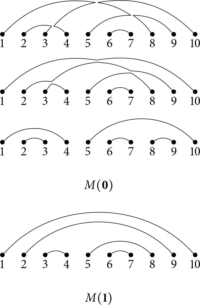
Figure 9: Examples for resolution of crossings with M shown in Figure 9.
Theorem 3.2 Let
 $M \in \mathcal {TC}_n$
. Then we have
$M \in \mathcal {TC}_n$
. Then we have
 $\varphi (M)=(M(\mathbf {0}),M(\mathbf {1}))$
, where
$\varphi (M)=(M(\mathbf {0}),M(\mathbf {1}))$
, where
 $M(\mathbf {0})$
and
$M(\mathbf {0})$
and
 $M(\mathbf {1})$
are identified with Dyck paths via the bijection
$M(\mathbf {1})$
are identified with Dyck paths via the bijection
 $\tau ^{-1}:\mathcal {NM}_n \to \mathcal {C}_n$
.
$\tau ^{-1}:\mathcal {NM}_n \to \mathcal {C}_n$
.
Proof We first recall the bijection between noncrossing matchings
 $\mathcal {NM}_n$
and Dyck paths
$\mathcal {NM}_n$
and Dyck paths
 $\mathcal {C}_n$
. A noncrossing matching
$\mathcal {C}_n$
. A noncrossing matching
 $M\in \mathcal {NM}_n$
is in bijection with a Dyck path
$M\in \mathcal {NM}_n$
is in bijection with a Dyck path
 $P\in \mathcal {C}_n$
if for all
$P\in \mathcal {C}_n$
if for all
 $j=1,\ldots ,2n$
, j is a left endpoint in M if and only if the jth step is an upstep in P.
$j=1,\ldots ,2n$
, j is a left endpoint in M if and only if the jth step is an upstep in P.
For a
 $3$
-noncrossing matching
$3$
-noncrossing matching
 $M\in \mathcal {TC}_n$
, write
$M\in \mathcal {TC}_n$
, write
 $\varphi (M)=(P_0\leq P_1)$
for notation purposes of this proof. Let
$\varphi (M)=(P_0\leq P_1)$
for notation purposes of this proof. Let
 $T_0,\ldots ,T_{2n}$
be the sequence of tableaux corresponding to M as defined above in this section. By construction,
$T_0,\ldots ,T_{2n}$
be the sequence of tableaux corresponding to M as defined above in this section. By construction,
 $T_j$
has one more entry than
$T_j$
has one more entry than
 $T_{j-1}$
if and only if j is a left endpoint in M. At the same time, we see from the construction of
$T_{j-1}$
if and only if j is a left endpoint in M. At the same time, we see from the construction of
 $M(\mathbf {1})$
that
$M(\mathbf {1})$
that
 $M(\mathbf {1})$
and M have the same set of left endpoints and right endpoints (see Figure 9 for a reference). Recall that the height of
$M(\mathbf {1})$
and M have the same set of left endpoints and right endpoints (see Figure 9 for a reference). Recall that the height of
 $P_1$
is given by the sizes of
$P_1$
is given by the sizes of
 $T_j$
’s, and by the bijection between noncrossing matchings and Dyck paths, we directly see that
$T_j$
’s, and by the bijection between noncrossing matchings and Dyck paths, we directly see that
 $P_1=M(\mathbf {1})$
.
$P_1=M(\mathbf {1})$
.
We use induction on n and on
 $|\mathrm {cr}(M)|$
to show that
$|\mathrm {cr}(M)|$
to show that
 $P_0$
and
$P_0$
and
 $M(\mathbf {0})$
are in bijection under
$M(\mathbf {0})$
are in bijection under
 $\tau $
. The base case
$\tau $
. The base case
 $n=1$
is trivial. The other base case is when
$n=1$
is trivial. The other base case is when
 $\mathrm {cr}(M)=\emptyset $
, i.e., M is noncrossing. Then the tableau
$\mathrm {cr}(M)=\emptyset $
, i.e., M is noncrossing. Then the tableau
 $T_0,\ldots ,T_{2n}$
all consist of a single row, so we can see that
$T_0,\ldots ,T_{2n}$
all consist of a single row, so we can see that
 $P_0=P_1$
is indeed in bijection with
$P_0=P_1$
is indeed in bijection with
 $M(\mathbf {0})=M(\mathbf {1})=M$
under
$M(\mathbf {0})=M(\mathbf {1})=M$
under
 $\tau $
.
$\tau $
.
For the inductive step, as
 $1$
is a left endpoint in M and
$1$
is a left endpoint in M and
 $2n$
is a right endpoint in M, there must exist a
$2n$
is a right endpoint in M, there must exist a
 $j\in \{1,\ldots ,2n-1\}$
such that j is a left endpoint and
$j\in \{1,\ldots ,2n-1\}$
such that j is a left endpoint and
 $j+1$
is a right endpoint in M. There are two possible cases: either
$j+1$
is a right endpoint in M. There are two possible cases: either
 $(j, j+1)$
are paired in the matching M, or they are not paired in M. In the first case where
$(j, j+1)$
are paired in the matching M, or they are not paired in M. In the first case where
 $(j,j+1)$
are paired M, let
$(j,j+1)$
are paired M, let
 $M'\in \mathcal {TC}_{n-1}$
be obtained from M by deleting the pair
$M'\in \mathcal {TC}_{n-1}$
be obtained from M by deleting the pair
 $(j,j+1)$
from M and flattening other entries. By the induction hypothesis, we have
$(j,j+1)$
from M and flattening other entries. By the induction hypothesis, we have
 $\varphi (M')=(P_0'\leq P_1')$
where
$\varphi (M')=(P_0'\leq P_1')$
where
 $P_0'$
is in bijection with
$P_0'$
is in bijection with
 $M'(\mathbf {0})$
. We know that
$M'(\mathbf {0})$
. We know that
 $M'(\mathbf {0})$
is obtained from
$M'(\mathbf {0})$
is obtained from
 $M(\mathbf {0})$
by removing the pair
$M(\mathbf {0})$
by removing the pair
 $(j,j+1)$
, so to show that
$(j,j+1)$
, so to show that
 $P_0$
and
$P_0$
and
 $M(\mathbf {0})$
are in bijection given that
$M(\mathbf {0})$
are in bijection given that
 $P_0'$
and
$P_0'$
and
 $M'(\mathbf {0})$
are in bijection, it suffices to show that
$M'(\mathbf {0})$
are in bijection, it suffices to show that
 $P_0'$
is obtained from
$P_0'$
is obtained from
 $P_0$
by deleting an upstep at j and a downstep at
$P_0$
by deleting an upstep at j and a downstep at
 $j+1$
. By definition of
$j+1$
. By definition of
 $T_0,\ldots ,T_{2n}$
,
$T_0,\ldots ,T_{2n}$
,
 $T_{j+1}$
is obtained from
$T_{j+1}$
is obtained from
 $T_{j+2}$
by inserting j, which is strictly larger than other values in
$T_{j+2}$
by inserting j, which is strictly larger than other values in
 $T_{j+2}$
so j gets inserted as the rightmost entry of the first row in
$T_{j+2}$
so j gets inserted as the rightmost entry of the first row in
 $T_{j+1}$
. Then
$T_{j+1}$
. Then
 $T_j$
is obtained from
$T_j$
is obtained from
 $T_{j+1}$
by deleting j from
$T_{j+1}$
by deleting j from
 $T_{j+1}$
, so
$T_{j+1}$
, so
 $T_j=T_{j+2}$
. This means that step j of
$T_j=T_{j+2}$
. This means that step j of
 $P_0$
is an upstep and step
$P_0$
is an upstep and step
 $j+1$
is a downstep. Moreover, the sequence of tableaux for
$j+1$
is a downstep. Moreover, the sequence of tableaux for
 $M'$
is
$M'$
is
 $T_0,\ldots ,T_{j}=T_{j+2},T_{j+3},\ldots ,T_{2n}$
so we conclude that
$T_0,\ldots ,T_{j}=T_{j+2},T_{j+3},\ldots ,T_{2n}$
so we conclude that
 $P_0'$
is obtained from
$P_0'$
is obtained from
 $P_0$
by deleting step j and
$P_0$
by deleting step j and
 $j+1$
and we are done.
$j+1$
and we are done.
In the second case where
 $(j,j+1)$
are not paired in the matching M. Suppose that j is paired with b and
$(j,j+1)$
are not paired in the matching M. Suppose that j is paired with b and
 $j+1$
is paired with a in M, where
$j+1$
is paired with a in M, where
 $b>j+1$
and
$b>j+1$
and
 $a<j$
. Let
$a<j$
. Let
 $M'$
be obtained from M by swapping the roles of j and
$M'$
be obtained from M by swapping the roles of j and
 $j+1$
, i.e.,
$j+1$
, i.e.,
 $M'$
is obtained from M by replacing the pair
$M'$
is obtained from M by replacing the pair
 $(a,j+1)$
and
$(a,j+1)$
and
 $(j,b)$
with
$(j,b)$
with
 $(a,j)$
and
$(a,j)$
and
 $(j+1,b)$
. We show that
$(j+1,b)$
. We show that
 $M'\in \mathcal {TC}_n$
. If there exist three strands
$M'\in \mathcal {TC}_n$
. If there exist three strands
 $A,B,C$
in
$A,B,C$
in
 $M'$
that intersect pairwise, then at least one of them is either
$M'$
that intersect pairwise, then at least one of them is either
 $(a,j)$
or
$(a,j)$
or
 $(j+1,b)$
. Say
$(j+1,b)$
. Say
 $A=(a,j)$
. Then as
$A=(a,j)$
. Then as
 $(j+1,b)$
does not intersect with
$(j+1,b)$
does not intersect with
 $(a,j)$
,
$(a,j)$
,
 $(j+1,b)$
does not belong to one of these strands. This means that
$(j+1,b)$
does not belong to one of these strands. This means that
 $(a,j+1)$
, B and C also intersect pairwise in M, contradicting
$(a,j+1)$
, B and C also intersect pairwise in M, contradicting
 $M\in \mathcal {TC}_n$
. Let
$M\in \mathcal {TC}_n$
. Let
 $T_0',\ldots ,T_{2n}'$
be the sequence of tableau associated with
$T_0',\ldots ,T_{2n}'$
be the sequence of tableau associated with
 $M'$
and let
$M'$
and let
 $\varphi (M')=(P_0'\leq P_1')$
. Let the shape of
$\varphi (M')=(P_0'\leq P_1')$
. Let the shape of
 $T_i$
be
$T_i$
be
 $(x_i,y_i)$
and the shape of
$(x_i,y_i)$
and the shape of
 $T_{i}'$
be
$T_{i}'$
be
 $(x_i',y_i')$
for
$(x_i',y_i')$
for
 $i=1,\ldots ,2n$
. The definition of
$i=1,\ldots ,2n$
. The definition of
 $M(\mathbf {0})$
gives
$M(\mathbf {0})$
gives
 $M(\mathbf {0})=M'(\mathbf {0})$
, as
$M(\mathbf {0})=M'(\mathbf {0})$
, as
 $M'$
can be viewed as resolving one crossing from M. As
$M'$
can be viewed as resolving one crossing from M. As
 $|cr(M')|<|cr(M)|$
, by induction hypothesis,
$|cr(M')|<|cr(M)|$
, by induction hypothesis,
 $P_0'$
and
$P_0'$
and
 $M'(\mathbf {0})$
are in bijection. To show that
$M'(\mathbf {0})$
are in bijection. To show that
 $P_0$
and
$P_0$
and
 $M(\mathbf {0})$
are in bijection, it suffices to show that
$M(\mathbf {0})$
are in bijection, it suffices to show that
 $P_0=P_0'$
, i.e.,
$P_0=P_0'$
, i.e.,
 $x_i-y_i=x_i'-y_i'$
for
$x_i-y_i=x_i'-y_i'$
for
 $i=1,\ldots ,2n.$
It is clear that
 $T_i=T_i'$
if
$T_i=T_i'$
if
 $i>b$
, and that
$i>b$
, and that
 $T_i$
has the same shape as
$T_i$
has the same shape as
 $T_i'$
if
$T_i'$
if
 $j+2\leq i\leq b$
, while replacing the value
$j+2\leq i\leq b$
, while replacing the value
 $j+1$
in
$j+1$
in
 $T_i'$
by j. For simplicity, we use
$T_i'$
by j. For simplicity, we use
 $\overline {j}$
to mean j in the tableaux
$\overline {j}$
to mean j in the tableaux
 $T_i$
, and
$T_i$
, and
 $j+1$
in
$j+1$
in
 $T_i'$
, for
$T_i'$
, for
 $i=1,\ldots ,2n$
. We see that
$i=1,\ldots ,2n$
. We see that
 $\overline {j}$
is the largest value in
$\overline {j}$
is the largest value in
 $T_{j+2}$
and
$T_{j+2}$
and
 $T_{j+2}'$
. Now,
$T_{j+2}'$
. Now,
 $T_{j+1}$
is obtained from
$T_{j+1}$
is obtained from
 $T_{j+2}$
by inserting a and
$T_{j+2}$
by inserting a and
 $T_{j}$
is obtained from
$T_{j}$
is obtained from
 $T_{j+1}$
by removing
$T_{j+1}$
by removing
 $\overline {j}$
, while
$\overline {j}$
, while
 $T_{j+1}'$
is obtained from
$T_{j+1}'$
is obtained from
 $T_{j+2}'$
by removing
$T_{j+2}'$
by removing
 $\overline {j}$
and
$\overline {j}$
and
 $T_{j}'$
is obtained from
$T_{j}'$
is obtained from
 $T_{j+1}'$
by inserting a. If
$T_{j+1}'$
by inserting a. If
 $\overline {j}$
is in the second row of
$\overline {j}$
is in the second row of
 $T_{j+2}$
and
$T_{j+2}$
and
 $T_{j+2}'$
, then a must be inserted in the first row of
$T_{j+2}'$
, then a must be inserted in the first row of
 $T_{j+2}$
, since otherwise, insertion of a will bump some value
$T_{j+2}$
, since otherwise, insertion of a will bump some value
 $c<\overline {j}$
to the second row of
$c<\overline {j}$
to the second row of
 $T_{j+2}$
, resulting in another bump that creates a third row, contradicting
$T_{j+2}$
, resulting in another bump that creates a third row, contradicting
 $T_{j+1}$
having at most
$T_{j+1}$
having at most
 $2$
rows. In this case,
$2$
rows. In this case,
 $(x_{j+1},y_{j+1})=(x_{j+2}+1, y_{j+2})$
while
$(x_{j+1},y_{j+1})=(x_{j+2}+1, y_{j+2})$
while
 $(x_{j+1}',y_{j+1}')=(x_{j+2},y_{j+2}-1)$
, satisfying
$(x_{j+1}',y_{j+1}')=(x_{j+2},y_{j+2}-1)$
, satisfying
 $x_{j+1}-y_{j+1}=x_{j+1}'-y_{j+1}'$
. Moreover, removing
$x_{j+1}-y_{j+1}=x_{j+1}'-y_{j+1}'$
. Moreover, removing
 $\overline {j}$
and inserting a commute on
$\overline {j}$
and inserting a commute on
 $T_{j+2}$
and
$T_{j+2}$
and
 $T_{j+2}'$
, so
$T_{j+2}'$
, so
 $T_i=T_i'$
for
$T_i=T_i'$
for
 $i\leq j$
. If
$i\leq j$
. If
 $\overline {j}$
is in the first row of
$\overline {j}$
is in the first row of
 $T_{j+2}$
and
$T_{j+2}$
and
 $T_{j+2}'$
, inserting a will increase the length of the second row, so
$T_{j+2}'$
, inserting a will increase the length of the second row, so
 $(x_{j+1},y_{j+1})=(x_{j+2},y_{j+2}+1)$
while
$(x_{j+1},y_{j+1})=(x_{j+2},y_{j+2}+1)$
while
 $(x_{j+1}',y_{j+1}')=(x_{j+2}-1,y_{j+2})$
, satisfying
$(x_{j+1}',y_{j+1}')=(x_{j+2}-1,y_{j+2})$
, satisfying
 $x_{j+1}-y_{j+1}=x_{j+1}'-y_{j+1}'$
. Moreover, whether a bumps
$x_{j+1}-y_{j+1}=x_{j+1}'-y_{j+1}'$
. Moreover, whether a bumps
 $\overline {j}$
to the second row or a bumps some other value to the second row, we directly see that removing
$\overline {j}$
to the second row or a bumps some other value to the second row, we directly see that removing
 $\overline {j}$
and inserting a commute. As a result,
$\overline {j}$
and inserting a commute. As a result,
 $x_i-y_i=x_i'-y_i'$
in all cases, concluding our proof.
$x_i-y_i=x_i'-y_i'$
in all cases, concluding our proof.
Proposition 3.3 For
 $M\in \mathcal {TC}_n$
and
$M\in \mathcal {TC}_n$
and
 $v\in \{0,1\}^{\mathrm {cr}(M)}$
,
$v\in \{0,1\}^{\mathrm {cr}(M)}$
,
 $M(v)\leq M(\mathbf {1})$
, with equality if and only if
$M(v)\leq M(\mathbf {1})$
, with equality if and only if
 $v=\mathbf {1}$
.
$v=\mathbf {1}$
.
Proof For a matching
 $M\in \mathcal {TC}_n$
and
$M\in \mathcal {TC}_n$
and
 $k=1,\ldots ,2n$
, let
$k=1,\ldots ,2n$
, let
 $l_k(M)$
denote the number of left endpoints among
$l_k(M)$
denote the number of left endpoints among
 $1,2,\ldots ,k$
in M, and let
$1,2,\ldots ,k$
in M, and let
 $r_k(M)$
denote the number of right endpoints among
$r_k(M)$
denote the number of right endpoints among
 $1,2,\ldots ,k$
. Recall that the corresponding Dyck path for M is the path that passes through
$1,2,\ldots ,k$
. Recall that the corresponding Dyck path for M is the path that passes through
 $(k,l_k(M)-r_k(M))$
for
$(k,l_k(M)-r_k(M))$
for
 $k=0,\ldots ,2n$
. Thus, to show
$k=0,\ldots ,2n$
. Thus, to show
 $M'\leq M$
, it suffices to show that
$M'\leq M$
, it suffices to show that
 $l_k(M')\leq l_k(M)$
for all k.
$l_k(M')\leq l_k(M)$
for all k.
Consider a planar drawing of M inside the rectangle
 $[1,2n]\times [0,1]$
, such that for a pair
$[1,2n]\times [0,1]$
, such that for a pair
 $(a,b)$
in M, where
$(a,b)$
in M, where
 $a<b$
, we connect the coordinate
$a<b$
, we connect the coordinate
 $(a,0)$
to
$(a,0)$
to
 $(b,0)$
via a curve
$(b,0)$
via a curve
 $\gamma _{a,b}:[0,1]\rightarrow [a,b]\times [0,1]$
such that
$\gamma _{a,b}:[0,1]\rightarrow [a,b]\times [0,1]$
such that
 $\gamma _{a,b}(0)=(a,0)$
,
$\gamma _{a,b}(0)=(a,0)$
,
 $\gamma _{a,b}(1)=(b,0)$
and that the projection of
$\gamma _{a,b}(1)=(b,0)$
and that the projection of
 $\gamma _{a,b}$
onto the first coordinate is bijective, i.e., we can view this curve as going from left to right. The matching shown in Figure 8 is such an example. We view
$\gamma _{a,b}$
onto the first coordinate is bijective, i.e., we can view this curve as going from left to right. The matching shown in Figure 8 is such an example. We view
 $M(v)$
as modifying and regrouping the curves in a small neighborhood around each crossing in M (see the top of Figure 9). Note that the crossings of M decompose the curves into segments. For each crossing z, there are four segments of curves touching z in the planar drawing of M, from the direction of NW, SW, NE, and SE.
$M(v)$
as modifying and regrouping the curves in a small neighborhood around each crossing in M (see the top of Figure 9). Note that the crossings of M decompose the curves into segments. For each crossing z, there are four segments of curves touching z in the planar drawing of M, from the direction of NW, SW, NE, and SE.
For
 $k=1,\ldots ,2n$
, the vertical line
$k=1,\ldots ,2n$
, the vertical line
 $x=k+0.5$
intersects the strands in the drawing of M with a left endpoint in
$x=k+0.5$
intersects the strands in the drawing of M with a left endpoint in
 $1,\ldots ,k$
and a right endpoint in
$1,\ldots ,k$
and a right endpoint in
 $k+1,\ldots ,n$
. There are
$k+1,\ldots ,n$
. There are
 $l_k(M)-r_k(M)$
number of such strands. Let
$l_k(M)-r_k(M)$
number of such strands. Let
 $\xi _1,\ldots ,\xi _h$
be the segments that intersect
$\xi _1,\ldots ,\xi _h$
be the segments that intersect
 $x=k+0.5$
, where
$x=k+0.5$
, where
 $h=l_k(M)-r_k(M)$
. Now, in any resolution of crossings
$h=l_k(M)-r_k(M)$
. Now, in any resolution of crossings
 $M(v)$
, there are
$M(v)$
, there are
 $l_k(M(v))-r_k(M(v))$
strands with a left endpoint in
$l_k(M(v))-r_k(M(v))$
strands with a left endpoint in
 $1,\ldots ,k$
and a right endpoint in
$1,\ldots ,k$
and a right endpoint in
 $k+1,\ldots ,n$
. Each such strand needs to contain at least one segment of
$k+1,\ldots ,n$
. Each such strand needs to contain at least one segment of
 $\xi _1,\ldots ,\xi _h$
, meaning that
$\xi _1,\ldots ,\xi _h$
, meaning that
 $l_k(M(v))-r_k(M(v))\leq h$
so
$l_k(M(v))-r_k(M(v))\leq h$
so
 $l_k(M(v))\leq l_k(M)=l_k(M(\mathbf {1}))$
. This means
$l_k(M(v))\leq l_k(M)=l_k(M(\mathbf {1}))$
. This means
 $M(v)\leq M(\mathbf {1})$
as desired.
$M(v)\leq M(\mathbf {1})$
as desired.
3.2
$3$
-noncrossing matchings and cactus networks

Proposition 3.4 Let
 $\tau \in \mathcal {M}_n$
be a matching. The followings are equivalent:
$\tau \in \mathcal {M}_n$
be a matching. The followings are equivalent:
-
(1)
$\tau \in \mathcal {TC}_n$
is a
$3$
-noncrossing matching; -
(2) all interior regions of (any) strand diagram of
$\tau $
have at least four sides; -
(3)
$\tau $
has a unique strand diagram; -
(4) there is a reduced cactus network
$\Gamma $
whose medial pairing is
$\tau $
such that
$\Gamma $
does not have any triangular faces and all interior vertices of
$\Gamma $
have degree at least
$4$
.


Proof We prove (1)
 $\Rightarrow $
(4)
$\Rightarrow $
(4)
 $\Rightarrow $
(3)
$\Rightarrow $
(3)
 $\Rightarrow $
(2)
$\Rightarrow $
(2)
 $\Rightarrow $
(1).
$\Rightarrow $
(1).
(1)
 $\Rightarrow $
(4). Assume
$\Rightarrow $
(4). Assume
 $\tau $
is a
$\tau $
is a
 $3$
-noncrossing matching. Take any strand diagram/medial graph of
$3$
-noncrossing matching. Take any strand diagram/medial graph of
 $\tau $
and recover a reduced cactus network
$\tau $
and recover a reduced cactus network
 $\Gamma $
as described in Section 2. As
$\Gamma $
as described in Section 2. As
 $\Gamma $
is reduced, no interior vertex has degree
$\Gamma $
is reduced, no interior vertex has degree
 $2$
. If
$2$
. If
 $\Gamma $
has a triangular face with edges
$\Gamma $
has a triangular face with edges
 $e_1,e_2,e_3$
, then this medial graph
$e_1,e_2,e_3$
, then this medial graph
 $G(\tau )$
has a triangular face given by
$G(\tau )$
has a triangular face given by
 $t_{e_1},t_{e_2},t_{e_3}$
; if
$t_{e_1},t_{e_2},t_{e_3}$
; if
 $\Gamma $
has an interior vertex of degree
$\Gamma $
has an interior vertex of degree
 $3$
, then it comes from a triangular face in the strand diagram. Both cases imply that there exists a triangular face in the strand diagram of
$3$
, then it comes from a triangular face in the strand diagram. Both cases imply that there exists a triangular face in the strand diagram of
 $\tau $
, which corresponds to three strands that cross pairwise, contradicting
$\tau $
, which corresponds to three strands that cross pairwise, contradicting
 $\tau $
being
$\tau $
being
 $3$
-noncrossing.
$3$
-noncrossing.
(4)
 $\Rightarrow $
(3). If
$\Rightarrow $
(3). If
 $\tau $
has two (or more) strand diagrams, then any corresponding reduced cactus network admits a
$\tau $
has two (or more) strand diagrams, then any corresponding reduced cactus network admits a
 $Y-\Delta $
move, by Proposition 2.1. But
$Y-\Delta $
move, by Proposition 2.1. But
 $\Gamma $
does not have any interior vertex of degree
$\Gamma $
does not have any interior vertex of degree
 $3$
or a triangular face. This is a contradiction.
$3$
or a triangular face. This is a contradiction.
(3)
 $\Rightarrow $
(2). If any strand diagram of
$\Rightarrow $
(2). If any strand diagram of
 $\tau $
has a region with three sides, i.e., a triangular face, then we can apply a local move of the form:
$\tau $
has a region with three sides, i.e., a triangular face, then we can apply a local move of the form: ![]() . This implies that
. This implies that
 $\tau $
has more than one strand diagram.
$\tau $
has more than one strand diagram.
(2)
 $\Rightarrow $
(1). If
$\Rightarrow $
(1). If
 $\tau $
is not
$\tau $
is not
 $3$
-noncrossing, then in a strand diagram of
$3$
-noncrossing, then in a strand diagram of
 $\tau $
, there are three strands that cross pairwise, forming an interior triangle. This triangle may not be a face, but any other strand that passes through this triangle creates a smaller triangle. Thus, any strand diagram of
$\tau $
, there are three strands that cross pairwise, forming an interior triangle. This triangle may not be a face, but any other strand that passes through this triangle creates a smaller triangle. Thus, any strand diagram of
 $\tau $
contains an interior triangular face.
$\tau $
contains an interior triangular face.
For a
 $3$
-noncrossing matching
$3$
-noncrossing matching
 $\xi \in \mathcal {TC}$
, let
$\xi \in \mathcal {TC}$
, let
 $\Gamma (\xi )$
be the corresponding reduced cactus network, which is unique by Proposition 3.4.
$\Gamma (\xi )$
be the corresponding reduced cactus network, which is unique by Proposition 3.4.
4 The grove algebra
$G_n$
and the Bush basis
$\{B_{\xi }\}$
for
$G_{n,2}$


Let
 $\mathfrak {I}_n\subset \mathbb {Z}[L_{\sigma }\:|\:\sigma \in \mathcal {NP}_n]$
be the ideal of polynomials in the variables
$\mathfrak {I}_n\subset \mathbb {Z}[L_{\sigma }\:|\:\sigma \in \mathcal {NP}_n]$
be the ideal of polynomials in the variables
 $\{L_{\sigma }\}_{\sigma \in \mathcal {NP}_n}$
that vanish on all electrical networks
$\{L_{\sigma }\}_{\sigma \in \mathcal {NP}_n}$
that vanish on all electrical networks
 $\Gamma $
, or equivalently, on all cactus networks
$\Gamma $
, or equivalently, on all cactus networks
 $\Gamma $
. Define the grove algebra (over
$\Gamma $
. Define the grove algebra (over
 $\mathbb {Z}$
) to be
$\mathbb {Z}$
) to be
 $$\begin{align*}G_n:=\mathbb{Z}[L_{\sigma}\:|\: \sigma\in\mathcal{NP}_n]/\mathfrak{I}_n,\end{align*}$$
which is a graded algebra by the degree of the polynomials, where we assign each variable
 $L_{\sigma }$
to have degree
$L_{\sigma }$
to have degree
 $1$
. Let the dth graded piece of
$1$
. Let the dth graded piece of
 $G_n$
be
$G_n$
be
 $G_{n,d}$
. We will describe
$G_{n,d}$
. We will describe
 $G_n \otimes {\mathbb C}$
in more algebro-geometric terms in Section 6.1.
$G_n \otimes {\mathbb C}$
in more algebro-geometric terms in Section 6.1.
In this section, we introduce a basis
 $\{B_\xi \:|\: \xi \in \mathcal {TC}_n\}$
of
$\{B_\xi \:|\: \xi \in \mathcal {TC}_n\}$
of
 $G_{n,2}$
indexed by 3-noncrossing matchings that exhibits cyclic symmetry. We first define
$G_{n,2}$
indexed by 3-noncrossing matchings that exhibits cyclic symmetry. We first define
 $B_\xi (\Gamma )$
for any cactus network
$B_\xi (\Gamma )$
for any cactus network
 $\Gamma $
and then lift them to
$\Gamma $
and then lift them to
 $G_{n,2}$
.
$G_{n,2}$
.
4.1 Definition of the Bush basis
$\{B_{\xi }\}$

Definition 4.1 A double grove H on boundary vertices
 $\bar 1,\bar 2,\ldots ,\bar n$
is a cactus graph where each edge has multiplicity
$\bar 1,\bar 2,\ldots ,\bar n$
is a cactus graph where each edge has multiplicity
 $1$
or
$1$
or
 $2$
(which we call a double edge).
$2$
(which we call a double edge).
Let
 $\mathbb {Z}\mathcal {TC}_n$
denote the free module with basis elements
$\mathbb {Z}\mathcal {TC}_n$
denote the free module with basis elements
 $\mathcal {TC}_n$
. For a double grove H, we define an invariant
$\mathcal {TC}_n$
. For a double grove H, we define an invariant
 $\alpha (H)\in \mathbb {Z}\mathcal {TC}_n$
by the following procedure.
$\alpha (H)\in \mathbb {Z}\mathcal {TC}_n$
by the following procedure.
Definition 4.2 For a cactus graph H with multiplicity (i.e., edges of H are allowed to have multiplicities being positive integers),
 $\alpha (H)$
is defined recursively as follows:
$\alpha (H)$
is defined recursively as follows:
-
(0) If some edge of H has multiplicity
$\geq 3$
, then
$\alpha (H)=0$
. -
(1) If all edges of H have multiplicity
$1$
and the medial pairing
$\tau (H)$
is a
$3$
-noncrossing matching
$\xi $
, i.e., H is reduced and does not have any interior vertex of degree equal to
$3$
or any triangular faces (see Proposition 3.4), then
$\alpha (H)=\xi $
. -
(2) If H has loops, then
$\alpha (H)=0$
. -
(3) If H has a double edge e, then
$\alpha (H)=\alpha (H')$
, where
$H'$
is obtained from H by contracting e. -
(4) If H has edges
$e_1,\ldots ,e_r$
of multiplicity
$1$
between the same pair of vertices, then
$\alpha (H)=0$
if
$r\geq 3$
, and
$\alpha (H)=2\alpha (H')$
where
$H'$
is obtained from H by contracting
$e_1$
(and removing
$e_2$
) if
$r=2$
. -
(5) If H has an interior leaf or an interior vertex with degree
$0$
, then
$\alpha (H)=0$
. -
(6) If H has an interior vertex v of degree
$2$
with distinct neighbors, then
$\alpha (H)=2\alpha (H')$
where
$H'$
is obtained from H by removing v. -
(7) If H has an interior vertex v of degree
$3$
with distinct neighbors
$v_1,v_2,v_3$
, then
$\alpha (H)=\alpha (H_1)+\alpha (H_2)+\alpha (H_3),$
where
$H_i$
is obtained from H by removing v together with the edges incident to it and adding the edge
$(v_{i+1},v_{i+2}),$
where the indices are taken modulo
$3$
. -
(8) If H has a triangular face (not necessarily in the interior) with vertices
$v_1,v_2,v_3$
, then
$\alpha (H)=\alpha (H_1)+\alpha (H_2)+\alpha (H_3),$
where
$H_i$
is obtained from H by identifying
$v_{i}$
with
$v_{i+1}$
and replacing the three edges by a single edge between
$v_i=v_{i+1}$
and
$v_{i+2}$
.


For
 $\xi \in \mathcal {TC}_n$
, let
$\xi \in \mathcal {TC}_n$
, let
 $\alpha (H)_{\xi }\in \mathbb {Z}$
denote the coefficient of
$\alpha (H)_{\xi }\in \mathbb {Z}$
denote the coefficient of
 $\xi $
in
$\xi $
in
 $\alpha (H)$
.
$\alpha (H)$
.

Figure 10: Moves (4), (6), (7), and (8) of Definition 4.2.
A visualization of some moves in Definition 4.2 is shown in Figure 10. It is clear that the procedure in Definition 4.2 terminates, as either the number of vertices or the number of edges strictly decreases after step. However, it is not immediately clear that
 $\alpha (H)$
is well-defined, i.e., the result of the recursion is independent of choices of moves. We show in Lemma 4.1 that indeed
$\alpha (H)$
is well-defined, i.e., the result of the recursion is independent of choices of moves. We show in Lemma 4.1 that indeed
 $\alpha (H)$
is well-defined.
$\alpha (H)$
is well-defined.
Lemma 4.1 For a double grove H,
 $\alpha (H)$
is well-defined. In other words,
$\alpha (H)$
is well-defined. In other words,
 $\alpha (H)$
does not depend on the order that we apply the moves in Definition 4.2.
$\alpha (H)$
does not depend on the order that we apply the moves in Definition 4.2.
Proof By Newman’s lemma (also commonly known as the diamond lemma) [Reference NewmanNew42], it suffices to show that for a cactus graph H with multiplicities, if there are two reduction moves m and
 $m'$
that can be applied to H resulting in
$m'$
that can be applied to H resulting in
 $\alpha (H)$
being assigned to
$\alpha (H)$
being assigned to
 $A=\sum c_i\alpha (H_i)$
and
$A=\sum c_i\alpha (H_i)$
and
 $A'=\sum c_i'\alpha (H_i')$
, then there are sequences of reduction moves that can be applied to A and
$A'=\sum c_i'\alpha (H_i')$
, then there are sequences of reduction moves that can be applied to A and
 $A'$
, respectively, such that the end results are the same. Depending on which types of moves m and
$A'$
, respectively, such that the end results are the same. Depending on which types of moves m and
 $m'$
are and which edges are involved in these moves, the number of cases to check is humongous, but most of them are very straightforward, including the situations where m and
$m'$
are and which edges are involved in these moves, the number of cases to check is humongous, but most of them are very straightforward, including the situations where m and
 $m'$
involve disjoint sets of edges and any combinations of moves (0)–(6). We check a few critical cases in this proof.
$m'$
involve disjoint sets of edges and any combinations of moves (0)–(6). We check a few critical cases in this proof.
Case 1: m and
 $m'$
are moves (7) applied to vertices v and
$m'$
are moves (7) applied to vertices v and
 $v'$
, respectively. Notice that if v and
$v'$
, respectively. Notice that if v and
 $v'$
are not adjacent, then moves (7) at v and
$v'$
are not adjacent, then moves (7) at v and
 $v'$
commute. So it suffices to look at the following local configuration in H, and apply the calculation in Figure 11, where we apply moves (7), (7), (6) in Definition 4.2 after move m. We see that the same result can be achieved if we apply move
$v'$
commute. So it suffices to look at the following local configuration in H, and apply the calculation in Figure 11, where we apply moves (7), (7), (6) in Definition 4.2 after move m. We see that the same result can be achieved if we apply move
 $m'$
first, as the end result in Figure 11 is symmetric horizontally.
$m'$
first, as the end result in Figure 11 is symmetric horizontally.

Figure 11: Case 1 of Lemma 4.1.
Case 2: m and
 $m'$
are moves (8) applied to the faces
$m'$
are moves (8) applied to the faces
 $v,x,y$
and faces
$v,x,y$
and faces
 $v',x,y$
, respectively. We have a similar calculation shown in Figure 12. Note that
$v',x,y$
, respectively. We have a similar calculation shown in Figure 12. Note that
 $v,x,y,v'$
may be incident to other edges and we will not draw these edges for simplicity of the visualization. We conclude that applying m first or
$v,x,y,v'$
may be incident to other edges and we will not draw these edges for simplicity of the visualization. We conclude that applying m first or
 $m'$
first can result in the same configuration via symmetry.
$m'$
first can result in the same configuration via symmetry.

Figure 12: Case 2 of Lemma 4.1.
Case 3: m is a move of type (7) applied to a vertex v and
 $m'$
is a move of type (8) applied to a triangular face
$m'$
is a move of type (8) applied to a triangular face
 $v,x,y$
. We consider the reductions separately for m and
$v,x,y$
. We consider the reductions separately for m and
 $m'$
in Figure 13 and observe the local confluence as desired. Notice that v has degree
$m'$
in Figure 13 and observe the local confluence as desired. Notice that v has degree
 $3$
, which is adjacent to the vertices
$3$
, which is adjacent to the vertices
 $x,y,z$
, while the vertices
$x,y,z$
, while the vertices
 $x,y,z$
can have more edges incident to them.
$x,y,z$
can have more edges incident to them.

Figure 13: Case 3 of Lemma 4.1.
The other cases involving some combinations of moves (0) to (6) of Definition 4.2 are tedious and straightforward to check so we omit them here.
Recall that for an edge-weighted graph H whose edges have multiplicities, its weight
 $\operatorname {\mathrm {wt}}(H)$
is given by the product of weights on the edges with multiplicity. For example, if some edge e has multiplicity
$\operatorname {\mathrm {wt}}(H)$
is given by the product of weights on the edges with multiplicity. For example, if some edge e has multiplicity
 $2$
, then it contributed
$2$
, then it contributed
 $\operatorname {\mathrm {wt}}(e)^2$
to
$\operatorname {\mathrm {wt}}(e)^2$
to
 $\operatorname {\mathrm {wt}}(H)$
.
$\operatorname {\mathrm {wt}}(H)$
.
Definition 4.3 For
 $\xi \in \mathcal {TC}_n$
, define
$\xi \in \mathcal {TC}_n$
, define
 $$\begin{align*}B_{\xi}(\Gamma):=\sum_{H\subset 2\Gamma}\alpha(H)_{\xi}\operatorname{\mathrm{wt}}(H)\end{align*}$$
for any cactus network
 $\Gamma $
, where the sum is over double groves H whose edges set is contained in that of
$\Gamma $
, where the sum is over double groves H whose edges set is contained in that of
 $\Gamma $
and
$\Gamma $
and
 $\alpha (H)_{\xi }$
is defined in Definition 4.2.
$\alpha (H)_{\xi }$
is defined in Definition 4.2.
Example 4.2. Consider the electrical network
 $\Gamma $
shown here with
$\Gamma $
shown here with
 $n=3$
that consists of an interior vertex x connected to
$n=3$
that consists of an interior vertex x connected to
 $\bar 1,\bar 2,\bar 3$
, with weights
$\bar 1,\bar 2,\bar 3$
, with weights
 $a,b,c$
, respectively:
$a,b,c$
, respectively:

Consider
 $\xi =\{(1,5),(2,6),(3,4)\}$
, for which we denote as
$\xi =\{(1,5),(2,6),(3,4)\}$
, for which we denote as
 $(15|26|34)$
for simplicity. In order to compute
$(15|26|34)$
for simplicity. In order to compute
 $B_{\xi }(\Gamma )$
, we need to sum over all
$B_{\xi }(\Gamma )$
, we need to sum over all
 $H\subset 2\Gamma $
, where there are
$H\subset 2\Gamma $
, where there are
 $27$
possibilities. However, notice that if H has
$27$
possibilities. However, notice that if H has
 $\leq 1$
edges, then (5) of Definition 4.2 implies
$\leq 1$
edges, then (5) of Definition 4.2 implies
 $\alpha (H)=0$
; and if H has
$\alpha (H)=0$
; and if H has
 $\geq 5$
edges counting with multiplicity, then after contracting once, some edge will have multiplicity
$\geq 5$
edges counting with multiplicity, then after contracting once, some edge will have multiplicity
 $\geq 3$
, implying that
$\geq 3$
, implying that
 $\alpha (H)=0$
as well. Here, we list the calculation of
$\alpha (H)=0$
as well. Here, we list the calculation of
 $\alpha (H)$
, for those
$\alpha (H)$
, for those
 $H\subset 2\Gamma $
such that
$H\subset 2\Gamma $
such that
 $\alpha (H)_{\xi }\neq 0$
.
$\alpha (H)_{\xi }\neq 0$
.

This calculation shows that
 $\alpha (\Gamma )=(15|26|34)+(13|24|56)+(12|35|46)$
so
$\alpha (\Gamma )=(15|26|34)+(13|24|56)+(12|35|46)$
so
 $\alpha (\Gamma )_\xi =1$
. We also have
$\alpha (\Gamma )_\xi =1$
. We also have

One can check that
 $\alpha (H)_{\xi }=0$
if H is not the above three choices. As a result, we compute that
$\alpha (H)_{\xi }=0$
if H is not the above three choices. As a result, we compute that
 $B_{\xi }(\Gamma )=abc+a^2c+ac^2$
.
$B_{\xi }(\Gamma )=abc+a^2c+ac^2$
.
4.2 Expansion of
$\{L_{\sigma }L_{\sigma '}\}$
into
$\{B_{\xi }\}$


We now work towards lifting
 $B_{\xi }$
’s to
$B_{\xi }$
’s to
 $G_{n,2}$
and showing that they form a basis of
$G_{n,2}$
and showing that they form a basis of
 $G_{n,2}$
. Recall that for a matching
$G_{n,2}$
. Recall that for a matching
 $M\in \mathcal {TC}_n$
and a vector
$M\in \mathcal {TC}_n$
and a vector
 $v\in \{0,1\}^{\mathrm {cr}(M)}$
,
$v\in \{0,1\}^{\mathrm {cr}(M)}$
,
 $M(v)\in \mathcal {NM}_n$
is the noncrossing matching obtained from resolving the crossings in M in the way specified by v, called a resolution of crossings (see Section 3). We say that such a resolution
$M(v)\in \mathcal {NM}_n$
is the noncrossing matching obtained from resolving the crossings in M in the way specified by v, called a resolution of crossings (see Section 3). We say that such a resolution
 $M(v)$
is valid if no internal loops result from the uncrossings, i.e., all segments are used.
$M(v)$
is valid if no internal loops result from the uncrossings, i.e., all segments are used.

Two loopless resolutions
 $M(v)$
and
$M(v)$
and
 $M(v')$
are called opposite if
$M(v')$
are called opposite if
 $v+v'=\mathbf {1}$
. Note that
$v+v'=\mathbf {1}$
. Note that
 $v+v'=\mathbf {1}$
means that the choices of uncrossings at every intersection in M for
$v+v'=\mathbf {1}$
means that the choices of uncrossings at every intersection in M for
 $M(v)$
and
$M(v)$
and
 $M(v')$
are different.
$M(v')$
are different.
Definition 4.4 For a
 $3$
-noncrossing matching
$3$
-noncrossing matching
 $\xi \in \mathcal {TC}_n$
, and a pair of noncrossing partitions
$\xi \in \mathcal {TC}_n$
, and a pair of noncrossing partitions
 $(\sigma ,\sigma ')\in \mathcal {NP}_n\times \mathcal {NP}_n$
, define
$(\sigma ,\sigma ')\in \mathcal {NP}_n\times \mathcal {NP}_n$
, define
 $a_{\xi ,(\sigma ,\sigma ')}$
to be the number of valid opposite loopless resolution of
$a_{\xi ,(\sigma ,\sigma ')}$
to be the number of valid opposite loopless resolution of
 $\xi $
that results in
$\xi $
that results in
 $(\sigma ,\sigma ')$
. In other words,
$(\sigma ,\sigma ')$
. In other words,
 $$\begin{align*}a_{\xi,(\sigma,\sigma')}:=\#\{v\in\{0,1\}^{\mathrm{cr}(\xi)}\:|\: \xi(v)=\tau(\sigma),\ \xi(\mathbf{1}{-}v)=\tau(\sigma')\text{ are both valid}\},\end{align*}$$
where
 $\tau (\sigma )$
is the noncrossing matching that corresponds to the noncrossing partition
$\tau (\sigma )$
is the noncrossing matching that corresponds to the noncrossing partition
 $\sigma $
as in Section 2.4.
$\sigma $
as in Section 2.4.
Lemma 4.3 For
 $\xi \in \mathcal {TC}_n$
and a pair of noncrossing partitions
$\xi \in \mathcal {TC}_n$
and a pair of noncrossing partitions
 $(\sigma ,\sigma ')\in \mathcal {NP}_n\times \mathcal {NP}_n$
,
$(\sigma ,\sigma ')\in \mathcal {NP}_n\times \mathcal {NP}_n$
,
 $a_{\xi ,(\sigma ,\sigma ')}$
equals the number of ways of splitting
$a_{\xi ,(\sigma ,\sigma ')}$
equals the number of ways of splitting
 $\Gamma (\xi )$
into two groves F and
$\Gamma (\xi )$
into two groves F and
 $F'$
with boundary partition
$F'$
with boundary partition
 $\sigma $
and
$\sigma $
and
 $\sigma '$
, respectively.
$\sigma '$
, respectively.
Proof Consider the cactus network
 $\Gamma =\Gamma (\xi )$
and the medial graph
$\Gamma =\Gamma (\xi )$
and the medial graph
 $G=G(\Gamma )$
of
$G=G(\Gamma )$
of
 $\xi $
together. For each crossing
$\xi $
together. For each crossing
 $x\in \mathrm {cr}(\xi )$
, there is a corresponding edge
$x\in \mathrm {cr}(\xi )$
, there is a corresponding edge
 $e_x$
in
$e_x$
in
 $\Gamma $
that passes through the this crossing. Consider two opposite resolution v and
$\Gamma $
that passes through the this crossing. Consider two opposite resolution v and
 $v'$
such that
$v'$
such that
 $v+v'=\mathbf {1}^{\mathrm {cr}(\xi )}$
. Correspondingly, we partition the edges of
$v+v'=\mathbf {1}^{\mathrm {cr}(\xi )}$
. Correspondingly, we partition the edges of
 $\Gamma $
into
$\Gamma $
into
 $F\sqcup F'$
such that at each crossing
$F\sqcup F'$
such that at each crossing
 $x\in \mathrm {cr}(\xi )$
, if the resolution
$x\in \mathrm {cr}(\xi )$
, if the resolution
 $\xi (v)$
does not intersect
$\xi (v)$
does not intersect
 $e_x$
, which looks like
$e_x$
, which looks like ![]() , then we assign
, then we assign
 $e_x$
to F, otherwise assign
$e_x$
to F, otherwise assign
 $e_x$
to
$e_x$
to
 $F'$
. This procedure is reversible, as any partition of the edge set of
$F'$
. This procedure is reversible, as any partition of the edge set of
 $\Gamma $
gives an opposite resolution.
$\Gamma $
gives an opposite resolution.
We also see that if F has a cycle, then
 $\xi (v)$
contains an interior loop inside this cycle. And if there is a connected component C of F not connected to the boundary, then
$\xi (v)$
contains an interior loop inside this cycle. And if there is a connected component C of F not connected to the boundary, then
 $\xi (v)$
also contains an interior loop following edges not assigned to F around C. Both situations are shown in Figure 14. Conversely, if
$\xi (v)$
also contains an interior loop following edges not assigned to F around C. Both situations are shown in Figure 14. Conversely, if
 $\xi (v)$
contains an interior loop, by tracing through the crossings in
$\xi (v)$
contains an interior loop, by tracing through the crossings in
 $\xi $
and the corresponding edges in
$\xi $
and the corresponding edges in
 $\Gamma $
around this loop, we recover one of the two situations described previously. As a result, the opposite resolutions are valid if and only if both F and
$\Gamma $
around this loop, we recover one of the two situations described previously. As a result, the opposite resolutions are valid if and only if both F and
 $F'$
are groves. So we obtain the desired statement.
$F'$
are groves. So we obtain the desired statement.

Figure 14: Invalid resolutions, where edges assigned to F are solid, edges assigned to
 $F'$
are dashed, and internal loops in
$F'$
are dashed, and internal loops in
 $\xi (v)$
are in red.
$\xi (v)$
are in red.
Theorem 4.4 For
 $\sigma ,\sigma '\in \mathcal {NP}_n$
and any cactus network
$\sigma ,\sigma '\in \mathcal {NP}_n$
and any cactus network
 $\Gamma $
,
$\Gamma $
,
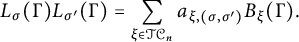 $$ \begin{align} L_{\sigma}(\Gamma)L_{\sigma'}(\Gamma)=\sum_{\xi\in\mathcal{TC}_n}a_{\xi,(\sigma,\sigma')}B_{\xi}(\Gamma). \end{align} $$
Proof By definition of
 $B_{\xi }(\Gamma )$
, the right-hand side of eq. (4.1) equals
$B_{\xi }(\Gamma )$
, the right-hand side of eq. (4.1) equals
 $$\begin{align*}\sum_{\xi\in\mathcal{TC}_n}a_{\xi,(\sigma,\sigma')}\sum_{H\subset 2\Gamma}\alpha(H)_{\xi}\operatorname{\mathrm{wt}}(H)=\sum_{H\subset2\Gamma}\operatorname{\mathrm{wt}}(H)\sum_{\xi\in\mathcal{TC}_n}a_{\xi,(\sigma,\sigma')}\alpha(H)_{\xi}.\end{align*}$$
Viewing every edge weight in
 $\Gamma $
as an indeterminate, we compare the coefficient of
$\Gamma $
as an indeterminate, we compare the coefficient of
 $\operatorname {\mathrm {wt}}(H)$
on both sides for every H. For a fixed
$\operatorname {\mathrm {wt}}(H)$
on both sides for every H. For a fixed
 $H\subset 2\Gamma $
, the coefficient of
$H\subset 2\Gamma $
, the coefficient of
 $\operatorname {\mathrm {wt}}(H)$
on the left-hand side
$\operatorname {\mathrm {wt}}(H)$
on the left-hand side
 $L_{\sigma }(\Gamma )L_{\sigma '}(\Gamma )$
is by definition the number of ways to partition H into
$L_{\sigma }(\Gamma )L_{\sigma '}(\Gamma )$
is by definition the number of ways to partition H into
 $F\sqcup F'$
such that F is a grove with boundary partition
$F\sqcup F'$
such that F is a grove with boundary partition
 $\sigma $
and
$\sigma $
and
 $F'$
is a grove with boundary partition
$F'$
is a grove with boundary partition
 $\sigma '$
. It suffices to show that this number equals
$\sigma '$
. It suffices to show that this number equals
 $\sum _{\xi \in \mathcal {TC}_n}a_{\xi ,(\sigma ,\sigma ')}\alpha (H)_{\xi }$
. The proof also explains the origin of Definition 4.2.
$\sum _{\xi \in \mathcal {TC}_n}a_{\xi ,(\sigma ,\sigma ')}\alpha (H)_{\xi }$
. The proof also explains the origin of Definition 4.2.
To split H into two groves
 $F\sqcup F'$
, there are a few easy steps of reduction. If some edge of H has multiplicity
$F\sqcup F'$
, there are a few easy steps of reduction. If some edge of H has multiplicity
 $\geq 3$
(which cannot happen at the very beginning) or H has a loop or H has an interior leaf, then clearly no such splittings are possible. These situations correspond to moves (0), (2), and (5) of Definition 4.2. Additionally, we can do the following reductions corresponding to moves (3), (4), and (6) of Definition 4.2:
$\geq 3$
(which cannot happen at the very beginning) or H has a loop or H has an interior leaf, then clearly no such splittings are possible. These situations correspond to moves (0), (2), and (5) of Definition 4.2. Additionally, we can do the following reductions corresponding to moves (3), (4), and (6) of Definition 4.2:
-
- If H has a double edge e, then both F and
$F'$
need to contain e, so we can simply assign e to both F and
$F'$
and then contract e. (Corresponds to move (3).) -
- If H has two edges
$e_1$
and
$e_2$
between the same pair of vertices, then one needs to be assigned to F and the other one to
$F'$
, so we can contract this edges and multiply the result by
$2$
. (Corresponds to move (4).) -
- If H has more than two edges between the same pair of vertices, then no assignment is possible. (Corresponds to move (4).)
-
- If H has an interior vertex of degree
$2$
with distinct neighbors, then these two edges must be assigned to F and
$F'$
, respectively, with both choices being symmetric and allowed. Therefore, we can remove this interior vertex and multiply the result by
$2$
. (Corresponds to move (6).)


Next, if H contains an interior vertex v of degree
 $3$
connected to
$3$
connected to
 $v_1,v_2,v_3$
, then to assign these three edges to F and
$v_1,v_2,v_3$
, then to assign these three edges to F and
 $F'$
, we need to partition these three edges into a group of one and a group of two. There are three ways of doing so. If
$F'$
, we need to partition these three edges into a group of one and a group of two. There are three ways of doing so. If
 $(v,v_1)$
is assigned to one of F and
$(v,v_1)$
is assigned to one of F and
 $F'$
and
$F'$
and
 $(v,v_2)$
and
$(v,v_2)$
and
 $(v,v_3)$
to the other, then effectively we are removing v (together with the three edges incident to it) from H, and adding an edge
$(v,v_3)$
to the other, then effectively we are removing v (together with the three edges incident to it) from H, and adding an edge
 $(v_2,v_3)$
to it, to obtain a smaller graph
$(v_2,v_3)$
to it, to obtain a smaller graph
 $H_2$
. For a partition of
$H_2$
. For a partition of
 $H_2$
into two groves
$H_2$
into two groves
 $F_2\sqcup F_2'$
, we can recover a partition of H into two groves
$F_2\sqcup F_2'$
, we can recover a partition of H into two groves
 $F\sqcup F'$
by assigning
$F\sqcup F'$
by assigning
 $(v,v_2)$
and
$(v,v_2)$
and
 $(v,v_3)$
to F if
$(v,v_3)$
to F if
 $(v_2,v_3)$
in
$(v_2,v_3)$
in
 $H_2$
is assigned to
$H_2$
is assigned to
 $F_2$
and vice versa. This justifies move (7) of Definition 4.2. The situation where H contains a triangular face, which is move (8), is similar.
$F_2$
and vice versa. This justifies move (7) of Definition 4.2. The situation where H contains a triangular face, which is move (8), is similar.
After all the reduction steps are performed, by Proposition 3.4, we are left with a graph H whose edges have multiplicity
 $1$
and H is the medial graph of some
$1$
and H is the medial graph of some
 $3$
-noncrossing matching
$3$
-noncrossing matching
 $\xi $
. This is move (1) of Definition 4.2. The integer
$\xi $
. This is move (1) of Definition 4.2. The integer
 $\alpha (H)_{\xi }$
is the number of ways that we end up in this situation. And the integer
$\alpha (H)_{\xi }$
is the number of ways that we end up in this situation. And the integer
 $a_{\xi ,(\sigma ,\sigma ')}$
is the number of ways to do the partition into two groves as desired, by Lemma 4.3. Summing over
$a_{\xi ,(\sigma ,\sigma ')}$
is the number of ways to do the partition into two groves as desired, by Lemma 4.3. Summing over
 $\xi \in \mathcal {TC}_n$
, we obtain the coefficient on the right-hand side of eq. (4.1), as desired.
$\xi \in \mathcal {TC}_n$
, we obtain the coefficient on the right-hand side of eq. (4.1), as desired.
Proposition 4.5 For each
 $\xi \in \mathcal {TC}_n$
, we can lift
$\xi \in \mathcal {TC}_n$
, we can lift
 $B_{\xi }$
to
$B_{\xi }$
to
 $G_{n,2}$
. Moreover,
$G_{n,2}$
. Moreover,
 $\{B_\xi \:|\: \xi \in \mathcal {TC}_n\}$
is a basis of
$\{B_\xi \:|\: \xi \in \mathcal {TC}_n\}$
is a basis of
 $G_{n,2}$
.
$G_{n,2}$
.
Proof Fixing n, we first show that
 $B_{\xi }$
’s are linearly independent. Recall that for each
$B_{\xi }$
’s are linearly independent. Recall that for each
 $\xi \in \mathcal {TC}_n$
, there is a corresponding cactus network
$\xi \in \mathcal {TC}_n$
, there is a corresponding cactus network
 $\Gamma (\xi )$
whose medial pairing is
$\Gamma (\xi )$
whose medial pairing is
 $\xi $
, and that the number of edges of
$\xi $
, and that the number of edges of
 $\Gamma (\xi )$
equals
$\Gamma (\xi )$
equals
 $\#\mathrm {cr}(\xi )$
, the number of crossings of
$\#\mathrm {cr}(\xi )$
, the number of crossings of
 $\xi $
. Consider the computation of
$\xi $
. Consider the computation of
 $\alpha (H)$
(Definition 4.2) for some
$\alpha (H)$
(Definition 4.2) for some
 $H\subset 2\Gamma (\xi )$
. Each reduction step in Definition 4.2 does not increase the number of edges. Moreover, if H contains any double edges, then those edges can be removed by step (3) of Definition 4.2. As a result, unless
$H\subset 2\Gamma (\xi )$
. Each reduction step in Definition 4.2 does not increase the number of edges. Moreover, if H contains any double edges, then those edges can be removed by step (3) of Definition 4.2. As a result, unless
 $H=\Gamma (\xi )$
,
$H=\Gamma (\xi )$
,
 $\alpha (H)\in \mathbb {Z} \mathcal {TC}_n$
is a linear combination of 3-noncrossing matchings with strictly fewer crossings than
$\alpha (H)\in \mathbb {Z} \mathcal {TC}_n$
is a linear combination of 3-noncrossing matchings with strictly fewer crossings than
 $\xi $
. And when
$\xi $
. And when
 $H=\Gamma (\xi )$
, we have
$H=\Gamma (\xi )$
, we have
 $\alpha (H)=\xi $
. This means that
$\alpha (H)=\xi $
. This means that
 $B_{\mu }(\Gamma (\xi ))=0$
if
$B_{\mu }(\Gamma (\xi ))=0$
if
 $\#\mathrm {cr}(\xi )\leq \#\mathrm {cr}(\mu )$
and
$\#\mathrm {cr}(\xi )\leq \#\mathrm {cr}(\mu )$
and
 $B_{\xi }(\Gamma (\xi ))=\operatorname {\mathrm {wt}}(\Gamma (\xi ))\neq 0$
.
$B_{\xi }(\Gamma (\xi ))=\operatorname {\mathrm {wt}}(\Gamma (\xi ))\neq 0$
.
If we have a nontrivial relation
 $\sum c_{\xi }B_{\xi }=0$
, by choosing the
$\sum c_{\xi }B_{\xi }=0$
, by choosing the
 $\xi $
with the smallest number of crossings with
$\xi $
with the smallest number of crossings with
 $c_{\xi }\neq 0$
and evaluating this relation
$c_{\xi }\neq 0$
and evaluating this relation
 $\sum c_{\xi }B_{\xi }=0$
on the cactus network
$\sum c_{\xi }B_{\xi }=0$
on the cactus network
 $\Gamma (\xi )$
, we obtain a contradiction. Thus,
$\Gamma (\xi )$
, we obtain a contradiction. Thus,
 $\{B_\xi \:|\: \xi \in \mathcal {TC}_n\}$
is linearly independent. In light of Theorem 4.4, this means that the matrix
$\{B_\xi \:|\: \xi \in \mathcal {TC}_n\}$
is linearly independent. In light of Theorem 4.4, this means that the matrix
 $M=\{a_{\xi ,(\sigma ,\sigma ')}\}$
whose rows are indexed by
$M=\{a_{\xi ,(\sigma ,\sigma ')}\}$
whose rows are indexed by
 $\xi \in \mathcal {TC}_n$
and columns indexed by
$\xi \in \mathcal {TC}_n$
and columns indexed by
 $(\sigma ,\sigma ')\in \mathcal {NP}_n\times \mathcal {NP}_n$
(which has way more columns than rows) has full rank. We can pick any representative for
$(\sigma ,\sigma ')\in \mathcal {NP}_n\times \mathcal {NP}_n$
(which has way more columns than rows) has full rank. We can pick any representative for
 $B_{\xi }\in G_{n,2}$
as a linear combination of
$B_{\xi }\in G_{n,2}$
as a linear combination of
 $L_{\sigma }L_{\sigma }$
’s by choosing a maximal invertible submatrix of M and invert it.
$L_{\sigma }L_{\sigma }$
’s by choosing a maximal invertible submatrix of M and invert it.
As elements in
 $G_{n,2}$
,
$G_{n,2}$
,
 $\{B_\xi \:|\: \xi \in \mathcal {TC}_n\}$
is a basis since they are linearly independent and they span
$\{B_\xi \:|\: \xi \in \mathcal {TC}_n\}$
is a basis since they are linearly independent and they span
 $G_{n,2}$
(Theorem 4.4).
$G_{n,2}$
(Theorem 4.4).
5 Connections to the Temperley–Lieb immanant
The Temperley–Lieb immanant
 $F_{\tau ,T}$
is defined by the second author [Reference LamLam15] as a function on a planar bipartite graph, or equivalently a function on the affine cone over the Grassmannian
$F_{\tau ,T}$
is defined by the second author [Reference LamLam15] as a function on a planar bipartite graph, or equivalently a function on the affine cone over the Grassmannian
 $\operatorname {\mathrm {Gr}}(k,n)$
. However, we take an orthogonal and self-contained approach and define
$\operatorname {\mathrm {Gr}}(k,n)$
. However, we take an orthogonal and self-contained approach and define
 $F_{\tau ,T}\in G_{n,2}$
as a linear combination of the Bush basis
$F_{\tau ,T}\in G_{n,2}$
as a linear combination of the Bush basis
 $\{B_{\xi }\:|\: \xi \in \mathcal {TC}_n\}$
.
$\{B_{\xi }\:|\: \xi \in \mathcal {TC}_n\}$
.
5.1 Temperley–Lieb immanants in terms of the Bush basis
Definition 5.1 A
 $(k,m)$
-partial noncrossing matching is a pair
$(k,m)$
-partial noncrossing matching is a pair
 $(\tau ,T)$
, such that
$(\tau ,T)$
, such that
 $\tau $
is a matching of a subset
$\tau $
is a matching of a subset
 $S(\tau )=S\subset \{1,2,\ldots ,m\}$
of even size that is noncrossing, i.e., if
$S(\tau )=S\subset \{1,2,\ldots ,m\}$
of even size that is noncrossing, i.e., if
 $[m]$
are arranged on a circle in order, then edges formed by
$[m]$
are arranged on a circle in order, then edges formed by
 $\tau $
won’t cross, and that
$\tau $
won’t cross, and that
 $T\subset [m]\setminus S$
with
$T\subset [m]\setminus S$
with
 $|S|+2|T|=2k$
.
$|S|+2|T|=2k$
.
Denote the set of
 $(k,m)$
-partial noncrossing matchings as
$(k,m)$
-partial noncrossing matchings as
 $\mathcal {A}_{k,m}$
. In the following, we take the parameters
$\mathcal {A}_{k,m}$
. In the following, we take the parameters
 $k=n-1$
and
$k=n-1$
and
 $m=2n$
.
$m=2n$
.
The framework of the next construction is similar to Section 5 of [Reference LamLam18]. For each
 $3$
-noncrossing matching
$3$
-noncrossing matching
 $\xi \in \mathcal {TC}_n$
, we define
$\xi \in \mathcal {TC}_n$
, we define
 $\beta (\xi )\in \mathbb {Z}\mathcal {A}_{n-1,2n}$
as follows.
$\beta (\xi )\in \mathbb {Z}\mathcal {A}_{n-1,2n}$
as follows.
Draw
 $\xi $
on a disk as a medial graph with n strands on
$\xi $
on a disk as a medial graph with n strands on
 $t_1,\ldots ,t_{2n}$
. We recover the information of cactus networks
$t_1,\ldots ,t_{2n}$
. We recover the information of cactus networks
 $\Gamma =\Gamma (\xi )$
and
$\Gamma =\Gamma (\xi )$
and
 $\Gamma ^{\vee }$
together in a single cactus, with a procedure similar to the process described in Section 2.3. Label the boundary vertices as
$\Gamma ^{\vee }$
together in a single cactus, with a procedure similar to the process described in Section 2.3. Label the boundary vertices as
 $1,2,\ldots ,2n$
such that i is between
$1,2,\ldots ,2n$
such that i is between
 $t_{i}$
and
$t_{i}$
and
 $t_{i+1}$
in clockwise order. These boundary vertices are colored black. The strands in
$t_{i+1}$
in clockwise order. These boundary vertices are colored black. The strands in
 $\xi $
divide the disk into regions. For each region, if there are boundary vertices in this region, we identify them together; and if there are no boundary vertices in this region, we add a black vertex for this interior region. These identifications result in a cactus
$\xi $
divide the disk into regions. For each region, if there are boundary vertices in this region, we identify them together; and if there are no boundary vertices in this region, we add a black vertex for this interior region. These identifications result in a cactus
 $S_{\zeta }$
. Make the intersections of strands in
$S_{\zeta }$
. Make the intersections of strands in
 $\xi $
into white vertices and connect each white vertex to the four black vertices that represent the four faces incident to it. Denote this cactus graph as
$\xi $
into white vertices and connect each white vertex to the four black vertices that represent the four faces incident to it. Denote this cactus graph as
 $N(\xi )$
. See Figure 15 for an example.
$N(\xi )$
. See Figure 15 for an example.

Figure 15: For
 $\xi =\{(1,9),(2,4),(3,6),(5,7),(8,10)\}$
, the bipartite graph
$\xi =\{(1,9),(2,4),(3,6),(5,7),(8,10)\}$
, the bipartite graph
 $N(\xi )$
with
$N(\xi )$
with
 $\xi $
draw in dashed lines,
$\xi $
draw in dashed lines,
 $\Gamma $
in black and
$\Gamma $
in black and
 $\Gamma ^{\vee }$
in red.
$\Gamma ^{\vee }$
in red.
Note that the graph
 $N(\xi )$
can be viewed as
$N(\xi )$
can be viewed as
 $\Gamma =\Gamma (\xi )$
and
$\Gamma =\Gamma (\xi )$
and
 $\Gamma ^{\vee }$
lying on top of each other, with intersections being the white vertices in
$\Gamma ^{\vee }$
lying on top of each other, with intersections being the white vertices in
 $N(\xi )$
. Each edge of
$N(\xi )$
. Each edge of
 $\Gamma $
and
$\Gamma $
and
 $\Gamma ^{\vee }$
consists of two edges in
$\Gamma ^{\vee }$
consists of two edges in
 $N(\xi )$
with endpoints having different colors, called “half-edges” in
$N(\xi )$
with endpoints having different colors, called “half-edges” in
 $\Gamma $
and
$\Gamma $
and
 $\Gamma ^{\vee }.$
Let
 $Z_1\sqcup \cdots \sqcup Z_r$
be the corresponding noncrossing partition of
$Z_1\sqcup \cdots \sqcup Z_r$
be the corresponding noncrossing partition of
 $[2n]$
so that we have r distinct vertices on the boundary of the cactus
$[2n]$
so that we have r distinct vertices on the boundary of the cactus
 $S_{\zeta }$
. Consider all the possible choices of A that consists of the following data:
$S_{\zeta }$
. Consider all the possible choices of A that consists of the following data:
-
(1) For every edge in
$\Gamma $
and
$\Gamma ^{\vee }$
, choose one of the two half-edges so that every interior vertex has degree
$2$
and every new boundary vertex
$Z_i$
has degree at most
$2$
. -
(2) The chosen edges can be partitioned into vertex-disjoint cycles and paths, whose endpoints are on the boundary. For each new boundary vertex
$Z_i$
of degree
$0$
, choose one vertex
$j\in Z_i$
and put the rest
$Z_i\setminus \{j\}$
in
$T(A)$
; for each
$Z_i$
and
$Z_{i'}$
of degree
$1$
that are the endpoints of a path, choose
$j\in Z_i$
and
$j'\in Z_{i'}$
, put this pair
$(j,j')$
in
$\tau (A)$
, and put the rest
$Z_i\setminus \{j\}$
and
$Z_{i'}\setminus \{j'\}$
in
$T(A)$
; for each
$Z_i$
of degree
$2$
, put
$Z_i$
in
$T(A)$
. Let
$\operatorname {\mathrm {cyc}}(A)$
be the number of cycles in A.


Lemma 5.1 For a choice A as above,
 $|\tau (A)|+2|T(A)|=2n-2$
.
$|\tau (A)|+2|T(A)|=2n-2$
.
Proof Keep the notations as above. The cactus
 $S_{\zeta }$
contains
$S_{\zeta }$
contains
 $1+2n-r$
circles, split into
$1+2n-r$
circles, split into
 $(1+2n-r)+n+\#\mathrm {cr}(\xi )$
regions by the n strands in
$(1+2n-r)+n+\#\mathrm {cr}(\xi )$
regions by the n strands in
 $\xi $
. Among these regions, there are
$\xi $
. Among these regions, there are
 $2n$
of them coming from the original boundary vertices, so we have
$2n$
of them coming from the original boundary vertices, so we have
 $1+n+\#\mathrm {cr}(\xi )-r$
interior regions, giving rise to
$1+n+\#\mathrm {cr}(\xi )-r$
interior regions, giving rise to
 $1+n+\#\mathrm {cr}(\xi )-r$
interior black vertices in
$1+n+\#\mathrm {cr}(\xi )-r$
interior black vertices in
 $N(\xi )$
. There are
$N(\xi )$
. There are
 $\#\mathrm {cr}(\xi )$
interior white vertices, so we have
$\#\mathrm {cr}(\xi )$
interior white vertices, so we have
 $1+n+2\#\mathrm {cr}(\xi )-r$
interior vertices and r boundary vertices in
$1+n+2\#\mathrm {cr}(\xi )-r$
interior vertices and r boundary vertices in
 $N(\xi )$
in total. From A, we selected
$N(\xi )$
in total. From A, we selected
 $2\#\mathrm {cr}(\xi )$
edges, contributing
$2\#\mathrm {cr}(\xi )$
edges, contributing
 $4\#\mathrm {cr}(\xi )$
to the total degree of all vertices. All interior vertices have degree
$4\#\mathrm {cr}(\xi )$
to the total degree of all vertices. All interior vertices have degree
 $2$
, so the sum of degrees of boundary vertices is
$2$
, so the sum of degrees of boundary vertices is
 $2r-2n-2$
. Assume that
$2r-2n-2$
. Assume that
 $2s$
of them have degree
$2s$
of them have degree
 $1$
, that
$1$
, that
 $r-n-s-1$
of them have degree
$r-n-s-1$
of them have degree
 $2$
, and that
$2$
, and that
 $n-s+1$
of them have degree
$n-s+1$
of them have degree
 $0$
. We then have
$0$
. We then have
 $|\tau (A)|=2s$
. Also by construction, we put every boundary vertex in
$|\tau (A)|=2s$
. Also by construction, we put every boundary vertex in
 $T(A)$
except one vertex of our choice from every new boundary vertex
$T(A)$
except one vertex of our choice from every new boundary vertex
 $Z_i$
with degree
$Z_i$
with degree
 $\leq 1$
. Thus,
$\leq 1$
. Thus,
 $T(A)=(2n)-(n+s+1)=n-s-1$
. This means
$T(A)=(2n)-(n+s+1)=n-s-1$
. This means
 $|\tau (A)|+2|T(A)|=2n-2$
as desired.
$|\tau (A)|+2|T(A)|=2n-2$
as desired.
Then we define
 $$\begin{align*}\beta(\xi):=\sum_{A}2^{\operatorname{\mathrm{cyc}}(A)}(\tau(A),T(A))\in\mathbb{Z}\mathcal{A}_{n-1,2n},\end{align*}$$
where the sum is over all selections A as above.
Example 5.2. First, consider an extreme example of
 $\xi =\{(1,2),(3,4),(5,6)\}$
with
$\xi =\{(1,2),(3,4),(5,6)\}$
with
 $n=3$
. The cactus
$n=3$
. The cactus
 $S_{\zeta }$
identifies
$S_{\zeta }$
identifies
 $2,4,6$
together. Since
$2,4,6$
together. Since
 $\xi $
is noncrossing, we do not need to select any half-edges, and the only choice that we make is choosing a
$\xi $
is noncrossing, we do not need to select any half-edges, and the only choice that we make is choosing a
 $2$
element subset of
$2$
element subset of
 $\{2,4,6\}$
to be
$\{2,4,6\}$
to be
 $T(A)$
. As a result,
$T(A)$
. As a result,
 $$\begin{align*}\beta(\{(1,2),(3,4),(5,6)\})=(\emptyset,\{2,4\})+(\emptyset,\{2,6\})+(\emptyset,\{4,6\}).\end{align*}$$
Example 5.3. Consider
 $\xi =\{(1,3),(2,5),(4,6)\}$
with two crossings, with
$\xi =\{(1,3),(2,5),(4,6)\}$
with two crossings, with
 $N(\xi )$
shown here.
$N(\xi )$
shown here.

All the
 $2^4=16$
selection of the half-edges are valid and we pick a few of them here:
$2^4=16$
selection of the half-edges are valid and we pick a few of them here:

with contributions
 $$\begin{align*}\beta(\xi)=(\{1,5\},\{6\})+(\{1,2,3,6\},\emptyset)+2(\emptyset,\{3,6\})+(\{2,6\},\{3\})+\cdots,\end{align*}$$
where the third term has a coefficient
 $2$
because there is a cycle.
$2$
because there is a cycle.
Definition 5.2 Let
 $(\tau ,T)\in \mathcal {A}_{n-1,2n}$
. Define
$(\tau ,T)\in \mathcal {A}_{n-1,2n}$
. Define
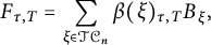 $$\begin{align*}F_{\tau,T}=\sum_{\xi\in\mathcal{TC}_n}\beta(\xi)_{\tau,T}B_{\xi},\end{align*}$$
where
 $\beta (\xi )_{\tau ,T}\in \mathbb {Z}_{\geq 0}$
is the coefficient of
$\beta (\xi )_{\tau ,T}\in \mathbb {Z}_{\geq 0}$
is the coefficient of
 $(\tau ,T)$
in
$(\tau ,T)$
in
 $\beta (\xi )$
.
$\beta (\xi )$
.
5.2 Concordance
We use the notion of concordance from Section 5 of [Reference LamLam18], to be explained further in Section 6.1. In Proposition 5.6, we will give a new derivation of the “electrical” Plücker relations (Proposition 5.35 of [Reference LamLam18]).
We say that an
 $(n-1)$
-element subset
$(n-1)$
-element subset
 $I\in \binom {[2n]}{n-1}$
is concordant with a noncrossing partition
$I\in \binom {[2n]}{n-1}$
is concordant with a noncrossing partition
 $\sigma $
if each part of
$\sigma $
if each part of
 $\sigma $
and each part of the dual partition
$\sigma $
and each part of the dual partition ![]() contains exactly one element not in I, viewing
contains exactly one element not in I, viewing
 $\sigma $
as a noncrossing partition on
$\sigma $
as a noncrossing partition on
 $1,3,\ldots ,2n-1$
and
$1,3,\ldots ,2n-1$
and ![]() on
on
 $2,4,\ldots ,2n$
. In general, we also say
$2,4,\ldots ,2n$
. In general, we also say
 $\sigma $
is concordant with I, or
$\sigma $
is concordant with I, or ![]() is concordant with I. Given
is concordant with I. Given
 $I\in \binom {[2n]}{n-1}$
, we use
$I\in \binom {[2n]}{n-1}$
, we use
 $\mathcal {E}(I)\subset \mathcal {NP}_n$
to denote the set of noncrossing partitions concordant with I.
$\mathcal {E}(I)\subset \mathcal {NP}_n$
to denote the set of noncrossing partitions concordant with I.
Example 5.4. Let
 $\sigma = (1,2,5\mid 3,4\mid 6)$
,
$\sigma = (1,2,5\mid 3,4\mid 6)$
, ![]() . Then
. Then
 $\sigma $
is concordant with the subset
$\sigma $
is concordant with the subset
 $\{3,4,7,9,12\}$
, but not concordant with the subset
$\{3,4,7,9,12\}$
, but not concordant with the subset
 $\{1,3,7,9,12\}$
(see Figure 16). We also draw the Dyck path interpretation for later purposes (Section 6).
$\{1,3,7,9,12\}$
(see Figure 16). We also draw the Dyck path interpretation for later purposes (Section 6).

Figure 16: Example of concordant and not concordant subsets.
For
 $I\in {2n\choose n-1}$
, define
$I\in {2n\choose n-1}$
, define
 $$ \begin{align} \Delta_I=\sum_{\sigma\in\mathcal{E}(I)}L_{\sigma}\in G_{n,1}. \end{align} $$
We say that a
 $(k,m)$
-partial noncrossing matching
$(k,m)$
-partial noncrossing matching
 $(\tau ,T)$
is compatible with
$(\tau ,T)$
is compatible with
 $I,J\in {m\choose k}$
if:
$I,J\in {m\choose k}$
if:
-
(1)
$\tau $
is a matching on
$(I\setminus J)\cup (J\setminus I)$
such that each edges contains one vertex in
$I\setminus J$
and the other vertex in
$J\setminus I$
; -
(2)
$T=I\cap J$
.


Theorem 5.5 For
 $I,J\in {2n\choose n-1}$
,
$I,J\in {2n\choose n-1}$
,
 $$ \begin{align} \Delta_I\Delta_J=\sum_{\tau,T}F_{\tau,T,} \end{align} $$
where the sum is over all
 $(\tau ,T)\in \mathcal {A}_{n-1,2n}$
compatible with
$(\tau ,T)\in \mathcal {A}_{n-1,2n}$
compatible with
 $I,J$
.
$I,J$
.
Proof Both sides are in
 $G_{n,2}$
. By Proposition 4.5, it suffices to compare the coefficient of
$G_{n,2}$
. By Proposition 4.5, it suffices to compare the coefficient of
 $B_{\xi }$
on both sides, for
$B_{\xi }$
on both sides, for
 $\xi \in \mathcal {TC}_n$
. We fix
$\xi \in \mathcal {TC}_n$
. We fix
 $I,J\in {2n\choose n-1}$
and
$I,J\in {2n\choose n-1}$
and
 $\xi \in \mathcal {TC}_n$
.
$\xi \in \mathcal {TC}_n$
.
By Theorem 4.4,
 $$\begin{align*}\Delta_I\Delta_J=\sum_{\sigma\in \mathcal{E}(I),\sigma'\in\mathcal{E}(J)}L_{\sigma}L_{\sigma'}=\sum_{\xi\in\mathcal{TC}_n}\sum_{\sigma\in \mathcal{E}(I),\sigma'\in\mathcal{E}(J)}a_{\xi,(\sigma,\sigma')}B_{\xi}.\end{align*}$$
The coefficient
 $a_{\xi ,(I,J)}:=\sum _{\sigma \in \mathcal {E}(I),\sigma '\in \mathcal {E}(J)}a_{\xi ,(\sigma ,\sigma ')}$
, by Lemma 4.3, equals the number of ways of splitting
$a_{\xi ,(I,J)}:=\sum _{\sigma \in \mathcal {E}(I),\sigma '\in \mathcal {E}(J)}a_{\xi ,(\sigma ,\sigma ')}$
, by Lemma 4.3, equals the number of ways of splitting
 $\Gamma :=\Gamma (\xi )$
into two groves
$\Gamma :=\Gamma (\xi )$
into two groves
 $F_I\sqcup F_J$
such that the boundary partition
$F_I\sqcup F_J$
such that the boundary partition
 $\sigma (F_I)$
is concordant with I and
$\sigma (F_I)$
is concordant with I and
 $\sigma (F_J)$
is concordant with J. Note that a splitting of
$\sigma (F_J)$
is concordant with J. Note that a splitting of
 $\Gamma $
corresponds to a splitting
$\Gamma $
corresponds to a splitting ![]() of
of
 $\Gamma ^{\vee }$
such that if
$\Gamma ^{\vee }$
such that if
 $e\in F_I$
, then its corresponding edge
$e\in F_I$
, then its corresponding edge
 $e^{\vee }$
in
$e^{\vee }$
in
 $\Gamma ^{\vee }$
belongs to
$\Gamma ^{\vee }$
belongs to
 $F_J$
. The boundary partitions of
$F_J$
. The boundary partitions of ![]() and
and ![]() is exactly the dual noncrossing partition
is exactly the dual noncrossing partition ![]() and
and ![]() , respectively, by definition. We will think about
, respectively, by definition. We will think about
 $F_I\sqcup F_J$
and
$F_I\sqcup F_J$
and ![]() simultaneously.
simultaneously.
For the right-hand side of eq. (5.2), summing over
 $(\tau ,T)$
compatible with
$(\tau ,T)$
compatible with
 $I,J$
,
$I,J$
,
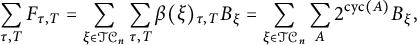 $$\begin{align*}\sum_{\tau, T}F_{\tau,T}=\sum_{\xi\in\mathcal{TC}_n}\sum_{\tau,T}\beta(\xi)_{\tau,T}B_{\xi}=\sum_{\xi\in\mathcal{TC}_n}\sum_{A}2^{\operatorname{\mathrm{cyc}}(A)}B_{\xi},\end{align*}$$
where the final sum is over choices of A, with each choice A consists of a selection of half-edges of
 $\Gamma $
and
$\Gamma $
and
 $\Gamma ^{\vee }$
and a certain selection of vertices in each group of boundary vertices
$\Gamma ^{\vee }$
and a certain selection of vertices in each group of boundary vertices
 $Z_i$
identified together (see the beginning of this section), such that
$Z_i$
identified together (see the beginning of this section), such that
 $\tau (A),T(A)$
is compatible with
$\tau (A),T(A)$
is compatible with
 $I,J$
.
$I,J$
.
To establish equality bijectively, we map each partition of groves
 $F_I\sqcup F_J$
to a choice of A described above, then we count the cardinality of the preimage of each A. This map
$F_I\sqcup F_J$
to a choice of A described above, then we count the cardinality of the preimage of each A. This map
 $\psi $
works as follows. The connected components of
$\psi $
works as follows. The connected components of ![]() give a partition
give a partition
 $[2n]$
into
$[2n]$
into
 $n+1$
parts (Lemma 2.2 of [Reference LamLam18]) and since
$n+1$
parts (Lemma 2.2 of [Reference LamLam18]) and since
 $\sigma (F)$
is concordant with I, there is exactly one vertex for each part that does not lie in I, called the root. We orient each tree in
$\sigma (F)$
is concordant with I, there is exactly one vertex for each part that does not lie in I, called the root. We orient each tree in ![]() toward the root (called a rooting) and for each edge
toward the root (called a rooting) and for each edge ![]() , choose the half-edge in
, choose the half-edge in
 $N(\xi )$
containing the source. Now, the selection A consists of these half-edges H, together with
$N(\xi )$
containing the source. Now, the selection A consists of these half-edges H, together with
 $T(A)=I\cap J$
and
$T(A)=I\cap J$
and
 $\tau (A)$
pairs up
$\tau (A)$
pairs up
 $I\setminus J$
and
$I\setminus J$
and
 $J\setminus I$
based on the paths formed by these half-edges (see Figure 17).
$J\setminus I$
based on the paths formed by these half-edges (see Figure 17).

Figure 17: The map
 $\psi $
in the proof of Theorem 5.5 with
$\psi $
in the proof of Theorem 5.5 with
 $\xi =(1,10|2,9|3,12|4,6|5,7|8,11)$
,
$\xi =(1,10|2,9|3,12|4,6|5,7|8,11)$
,
 $I=\{1,5,7,8,11\}$
,
$I=\{1,5,7,8,11\}$
,
 $J=\{3,4,7,9,12\}.$
Top left:
$J=\{3,4,7,9,12\}.$
Top left: ![]() ; top right:
; top right: ![]() ; bottom: the selection A in
; bottom: the selection A in
 $N(\xi )$
with edges in
$N(\xi )$
with edges in
 $\Gamma $
colored in black and edges in
$\Gamma $
colored in black and edges in
 $\Gamma ^{\vee }$
colored in red.
$\Gamma ^{\vee }$
colored in red.
We first justify that this map
 $\psi $
is well-defined, i.e., the selection A obtained satisfies that every internal vertex has degree
$\psi $
is well-defined, i.e., the selection A obtained satisfies that every internal vertex has degree
 $2$
in H, every boundary vertex has degree at most
$2$
in H, every boundary vertex has degree at most
 $2$
in H, and that the pair
$2$
in H, and that the pair
 $(\tau (A),T(A))$
is compatible with
$(\tau (A),T(A))$
is compatible with
 $I,J$
. Recall that
$I,J$
. Recall that
 $H\subset N(\xi )$
is the set of half-edges that we selected. To begin with, each white interior vertex has degree
$H\subset N(\xi )$
is the set of half-edges that we selected. To begin with, each white interior vertex has degree
 $2$
. Each black interior vertex is not a root in its connected component in
$2$
. Each black interior vertex is not a root in its connected component in ![]() so it has outdegree
so it has outdegree
 $1$
in the rooting, gaining one degree in H; similarly, it gains one degree in H from
$1$
in the rooting, gaining one degree in H; similarly, it gains one degree in H from ![]() so it has degree
so it has degree
 $2$
in total. Likewise, each boundary black vertex is either a root in
$2$
in total. Likewise, each boundary black vertex is either a root in ![]() , in which case it gains no degree in H, or not a root in
, in which case it gains no degree in H, or not a root in ![]() , in which case it gains one degree in H. So considering
, in which case it gains one degree in H. So considering ![]() as well, each boundary vertex has degree
as well, each boundary vertex has degree
 $\leq 2$
.
$\leq 2$
.
The selection A also consists of the data of
 $\tau (A)$
and
$\tau (A)$
and
 $T(A)$
and we need to show the following: First, from
$T(A)$
and we need to show the following: First, from
 $\psi $
,
$\psi $
,
 $\tau (A)$
can be chosen so that
$\tau (A)$
can be chosen so that
 $I\setminus J$
is paired with
$I\setminus J$
is paired with
 $J\setminus I$
given by the paths formed by the half-edges described above; and second,
$J\setminus I$
given by the paths formed by the half-edges described above; and second,
 $T(A)=I\cap J$
consists of
$T(A)=I\cap J$
consists of
 $|Z_k|-1$
vertices from
$|Z_k|-1$
vertices from
 $Z_k$
if
$Z_k$
if
 $Z_k$
is of degree
$Z_k$
is of degree
 $0$
or
$0$
or
 $1$
in H and consists of all vertices from
$1$
in H and consists of all vertices from
 $Z_k$
if
$Z_k$
if
 $Z_k$
is of degree
$Z_k$
is of degree
 $2$
in H, where
$2$
in H, where
 $Z_1,\ldots ,Z_m$
is the set of boundary vertices in the cactus. The claim concerning
$Z_1,\ldots ,Z_m$
is the set of boundary vertices in the cactus. The claim concerning
 $T(A)$
is clear by counting:
$T(A)$
is clear by counting:
 $v\in [2n]$
contributes degree x to
$v\in [2n]$
contributes degree x to
 $Z_k\ni v$
if v appears x times in
$Z_k\ni v$
if v appears x times in
 $I\cup J$
as a multiset. As for
$I\cup J$
as a multiset. As for
 $\tau (A)$
, it suffices to show that we cannot form a path with the two endpoints both in
$\tau (A)$
, it suffices to show that we cannot form a path with the two endpoints both in
 $I\setminus J$
. This is done by a parity argument. Notice that as we traverse half-edges consecutively in a path or a cycle of H, we alternate between black vertices and white vertices, and alternate between edges in
$I\setminus J$
. This is done by a parity argument. Notice that as we traverse half-edges consecutively in a path or a cycle of H, we alternate between black vertices and white vertices, and alternate between edges in ![]() and edges in
and edges in ![]() . Thus, if a path in H starts with a vertex v and an edge in
. Thus, if a path in H starts with a vertex v and an edge in ![]() , ends with a vertex w and an edge in
, ends with a vertex w and an edge in ![]() , then we know that
, then we know that
 $v\notin I$
and
$v\notin I$
and
 $w\notin J$
, meaning that
$w\notin J$
, meaning that
 $v\in J$
and
$v\in J$
and
 $w\in I$
as they need to have degree
$w\in I$
as they need to have degree
 $1$
. This shows that
$1$
. This shows that
 $(\tau (A),T(A))$
is compatible with
$(\tau (A),T(A))$
is compatible with
 $I,J$
.
$I,J$
.
Now fix a selection A such that
 $(\tau (A),T(A))$
is compatible with
$(\tau (A),T(A))$
is compatible with
 $I,J$
. We count the number of partitions of
$I,J$
. We count the number of partitions of
 $\Gamma $
into groves
$\Gamma $
into groves
 $F_I\sqcup F_J$
such that
$F_I\sqcup F_J$
such that
 $\sigma (F_I),\sigma (F_J)$
are concordant with
$\sigma (F_I),\sigma (F_J)$
are concordant with
 $I,J$
, respectively. For each path P in A, we can without loss of generality assume that it starts with
$I,J$
, respectively. For each path P in A, we can without loss of generality assume that it starts with
 $v\in I\setminus J$
and ends with
$v\in I\setminus J$
and ends with
 $w\in J\setminus I$
, as
$w\in J\setminus I$
, as
 $\tau (A)$
is a matching that pairs
$\tau (A)$
is a matching that pairs
 $I\setminus J$
with
$I\setminus J$
with
 $J\setminus I$
. As we traverse the half-edges in P, the first edge incident to v needs to be assigned to
$J\setminus I$
. As we traverse the half-edges in P, the first edge incident to v needs to be assigned to ![]() for a rooting to exist. Then the half-edges must alternate between
for a rooting to exist. Then the half-edges must alternate between ![]() and
and ![]() since for a rooting to exist, each internal black vertex has outdegree
since for a rooting to exist, each internal black vertex has outdegree
 $1$
in both
$1$
in both ![]() and
and ![]() . This alternating property allows us to assign all edges along this path P. Likewise, every cycle C in A has two possible assignments to
. This alternating property allows us to assign all edges along this path P. Likewise, every cycle C in A has two possible assignments to ![]() and
and ![]() via the alternating property (see Figure 18). Thus, every edge in
via the alternating property (see Figure 18). Thus, every edge in
 $\Gamma $
and
$\Gamma $
and
 $\Gamma ^{\vee }$
is now assigned to either
$\Gamma ^{\vee }$
is now assigned to either ![]() or
or ![]() . Notice that every directed tree whose internal vertices have outdegree
. Notice that every directed tree whose internal vertices have outdegree
 $1$
has a leaf that is the unique source, i.e., a root. So the concordant property with I and J is exactly the same as the existence of a rooting. All
$1$
has a leaf that is the unique source, i.e., a root. So the concordant property with I and J is exactly the same as the existence of a rooting. All
 $2^{\operatorname {\mathrm {cyc}}(A)}$
choices satisfy the requirement. This finishes the comparison of coefficients of
$2^{\operatorname {\mathrm {cyc}}(A)}$
choices satisfy the requirement. This finishes the comparison of coefficients of
 $B_{\xi }$
on both sides of eq. (5.2) as desired.
$B_{\xi }$
on both sides of eq. (5.2) as desired.
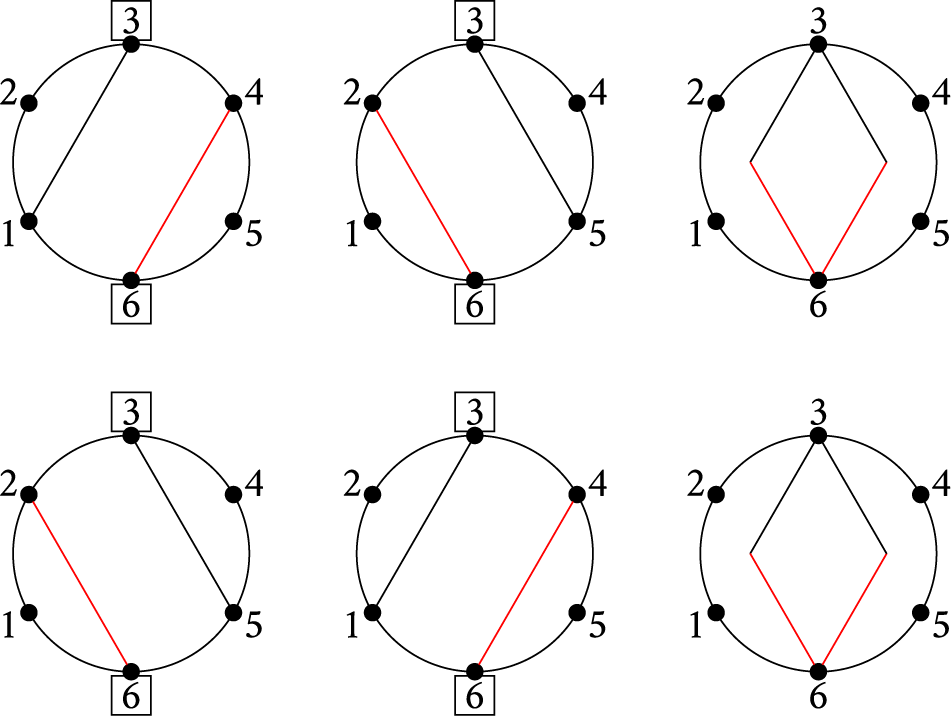
Figure 18: An example of two partitions achieving the same cycle in
 $N(\xi )$
with
$N(\xi )$
with
 $\xi =(13|25|46)$
,
$\xi =(13|25|46)$
,
 $I,J=\{3,6\}$
. Left:
$I,J=\{3,6\}$
. Left: ![]() ; middle:
; middle: ![]() ; right: the same selection A of
; right: the same selection A of
 $N(\xi )$
.
$N(\xi )$
.
We have now established the following commutative diagram of various expansions:

The existence of
 $F_{\tau ,T}$
’s satisfying Theorem 5.5 is equivalent to the Plücker relations of the Plücker ring (see Theorems 3.1 and 3.10 of [Reference LamLam15]). Using eq. (5.1), we deduce the “electrical” Plücker relations.
$F_{\tau ,T}$
’s satisfying Theorem 5.5 is equivalent to the Plücker relations of the Plücker ring (see Theorems 3.1 and 3.10 of [Reference LamLam15]). Using eq. (5.1), we deduce the “electrical” Plücker relations.
Proposition 5.6 (Proposition 5.35 of [Reference LamLam18])
For each
 $1\leq k < n-1$
and each
$1\leq k < n-1$
and each
 $I = \{i_1 < i_2 < \dots < i_{n-1}\}, J = \{j_1 < j_2 < \dots < j_{n-1}\}$
, we have
$I = \{i_1 < i_2 < \dots < i_{n-1}\}, J = \{j_1 < j_2 < \dots < j_{n-1}\}$
, we have
 $$\begin{align*}\sum_{\sigma\in \mathcal{E}(I),\kappa\in \mathcal{E}(J)}L_{\sigma}L_{\kappa} = \sum_{I', J'}(-1)^{a(I', J')}\sum_{\sigma\in \mathcal{E}(I'), \kappa\in \mathcal{E}(J')}L_\sigma L_\kappa,\end{align*}$$
where:
-
(1) the summation is over
$I', J'$
obtained from swapping the last k indices in J with any k indices in I, keeping the order in both; -
(2)
$a(I', J')$
is the total number of swaps needed to put both subsets
$I'$
and
$J'$
in order.


6 Tableaux basis of the grove algebra
In this section, we provide a basis of
 $G_n$
, building on results in [Reference Bychkov, Gorbounov, Kazakov and TalalaevBGKT21, Reference Chepuri, George and SpeyerCGS21]. We will select a set of relations R from Proposition 5.6 and show that R is a Gröbner basis of the ideal
$G_n$
, building on results in [Reference Bychkov, Gorbounov, Kazakov and TalalaevBGKT21, Reference Chepuri, George and SpeyerCGS21]. We will select a set of relations R from Proposition 5.6 and show that R is a Gröbner basis of the ideal
 $\mathfrak {I}_n$
, which is defined to be the ideal of polynomials in the variables
$\mathfrak {I}_n$
, which is defined to be the ideal of polynomials in the variables
 $\{L_{\sigma }\}_{\sigma \in \mathcal {NP}_n}$
that vanish on all electrical networks
$\{L_{\sigma }\}_{\sigma \in \mathcal {NP}_n}$
that vanish on all electrical networks
 $\Gamma $
.
$\Gamma $
.
We work over
 ${\mathbb C}$
in this section, and
${\mathbb C}$
in this section, and
 $G_n$
denotes
$G_n$
denotes
 $G_n \otimes {\mathbb C}$
.
$G_n \otimes {\mathbb C}$
.
6.1 Embedding into the Grassmannian
Let
 $R(n-1,2n)$
denote the Plücker ring, the homogeneous coordinate ring of the Grassmannian
$R(n-1,2n)$
denote the Plücker ring, the homogeneous coordinate ring of the Grassmannian
 $\operatorname {\mathrm {Gr}}(n-1,2n)$
.
$\operatorname {\mathrm {Gr}}(n-1,2n)$
.
Theorem 6.1 The formula
 $$ \begin{align} \Delta_I=\sum_{\sigma\in\mathcal{E}(I)}L_{\sigma}\in G_{n,1} () \end{align} $$
induces a graded ring homomorphism
 $\iota ^*: R(n-1,2n) \to G_n$
.
$\iota ^*: R(n-1,2n) \to G_n$
.
Proof Let
 $\pi : {\mathbb C}[\Delta _I \mid I \in \binom {[2n]}{n-1}] \to G_n$
be the ring homomorphism given by the eq. (5.1). The ring
$\pi : {\mathbb C}[\Delta _I \mid I \in \binom {[2n]}{n-1}] \to G_n$
be the ring homomorphism given by the eq. (5.1). The ring
 $R(n-1,2n)$
is the quotient of
$R(n-1,2n)$
is the quotient of
 ${\mathbb C}[\Delta _I]$
by the Plücker ideal generated by the Plücker relations. We need to check that the Plücker ideal belongs to the kernel of
${\mathbb C}[\Delta _I]$
by the Plücker ideal generated by the Plücker relations. We need to check that the Plücker ideal belongs to the kernel of
 $\pi $
.
$\pi $
.
It is shown in Theorem 3.10 of [Reference LamLam15] that the existence of elements
 $F_{\tau ,T}$
satisfying our Theorem 5.5 implies the Plücker relations, at least set-theoretically. Since the ring
$F_{\tau ,T}$
satisfying our Theorem 5.5 implies the Plücker relations, at least set-theoretically. Since the ring
 $G_n$
has no nilpotents, it follows that the entire Plücker ideal belongs to the kernel of
$G_n$
has no nilpotents, it follows that the entire Plücker ideal belongs to the kernel of
 $\pi $
.
$\pi $
.
The ring homomorphism
 $\iota ^*: R(n-1,2n) \to G_n$
induces a morphism between projective varieties
$\iota ^*: R(n-1,2n) \to G_n$
induces a morphism between projective varieties
 $$ \begin{align*}\mathrm{Proj}(G_n) \to \mathrm{Proj}(R(n-1,2n)).\end{align*} $$
Indeed, this is exactly the embedding
 $\iota $
of electrical networks into the Grassmannian
$\iota $
of electrical networks into the Grassmannian
 $\operatorname {\mathrm {Gr}}(n-1,2n)$
constructed in [Reference LamLam18], and our results give a new proof of this embedding. Note that in [Reference LamLam18], the eq. (5.1) is a theorem, whereas for us it is a definition.
$\operatorname {\mathrm {Gr}}(n-1,2n)$
constructed in [Reference LamLam18], and our results give a new proof of this embedding. Note that in [Reference LamLam18], the eq. (5.1) is a theorem, whereas for us it is a definition.
The embedding is constructed in [Reference LamLam18] as follows. Recall that
 $C_n$
denotes the nth Catalan number. Let
$C_n$
denotes the nth Catalan number. Let
 $M = (M_{I\sigma })$
be the
$M = (M_{I\sigma })$
be the
 $\binom {2n}{n-1} \times C_n$
matrix of
$\binom {2n}{n-1} \times C_n$
matrix of
 $1$
-s and
$1$
-s and
 $0$
-s, with
$0$
-s, with
 $1$
-s in the entries corresponding to pairs
$1$
-s in the entries corresponding to pairs
 $(I,\sigma ) \in \binom {[2n]}{n-1} \times \mathcal {NP}_n$
that are concordant. Let
$(I,\sigma ) \in \binom {[2n]}{n-1} \times \mathcal {NP}_n$
that are concordant. Let
 $\mathcal {X}_n = H \cap \operatorname {\mathrm {Gr}}(n-1,2n)$
be the linear slice of the Grassmannian, where
$\mathcal {X}_n = H \cap \operatorname {\mathrm {Gr}}(n-1,2n)$
be the linear slice of the Grassmannian, where
 $H \subset {\mathbb P}^{\binom {2n}{n-1}-1}$
is the projective subspace given by the image of the matrix M. It is shown in [Reference LamLam18] that
$H \subset {\mathbb P}^{\binom {2n}{n-1}-1}$
is the projective subspace given by the image of the matrix M. It is shown in [Reference LamLam18] that
 $\mathcal {X}_{n,\geq 0}:= \mathcal {X}_n \cap \operatorname {\mathrm {Gr}}(n-1,2n)_{\geq 0}$
is isomorphic to the compactified space of electrical networks. Since
$\mathcal {X}_{n,\geq 0}:= \mathcal {X}_n \cap \operatorname {\mathrm {Gr}}(n-1,2n)_{\geq 0}$
is isomorphic to the compactified space of electrical networks. Since
 $\mathcal {X}_{n,\geq 0}$
is Zariski-dense in
$\mathcal {X}_{n,\geq 0}$
is Zariski-dense in
 $\mathcal {X}$
, we have the following result.
$\mathcal {X}$
, we have the following result.
Proposition 6.2 The homogeneous coordinate ring of
 $\mathcal {X}$
is naturally isomorphic to the grove algebra
$\mathcal {X}$
is naturally isomorphic to the grove algebra
 $G_n$
. The ring homomorphism
$G_n$
. The ring homomorphism
 $\pi :R(n-1,2n) \to G_n$
in Theorem 6.1 induces the embedding
$\pi :R(n-1,2n) \to G_n$
in Theorem 6.1 induces the embedding
 $\iota : \mathcal {X}_n \hookrightarrow \operatorname {\mathrm {Gr}}(n-1,2n)$
of [Reference LamLam18].
$\iota : \mathcal {X}_n \hookrightarrow \operatorname {\mathrm {Gr}}(n-1,2n)$
of [Reference LamLam18].
6.2 Electrical networks and the Lagrangian Grassmannian
The subvariety
 $\mathcal {X}_n$
was further studied in the works of Chepuri, George, and Speyer [Reference Chepuri, George and SpeyerCGS21] and by Bychkov, Gorbounov, Kazakov, and Talalaev [Reference Bychkov, Gorbounov, Kazakov and TalalaevBGKT21], who established the following result.
$\mathcal {X}_n$
was further studied in the works of Chepuri, George, and Speyer [Reference Chepuri, George and SpeyerCGS21] and by Bychkov, Gorbounov, Kazakov, and Talalaev [Reference Bychkov, Gorbounov, Kazakov and TalalaevBGKT21], who established the following result.
Theorem 6.3 The subvariety
 $\mathcal {X}_n$
is isomorphic to the Lagrangian Grassmannian
$\mathcal {X}_n$
is isomorphic to the Lagrangian Grassmannian
 $\operatorname {\mathrm {LG}}(n-1,2n-2)$
.
$\operatorname {\mathrm {LG}}(n-1,2n-2)$
.
The appearance of the symplectic group in the study of electrical networks earlier appeared in [Reference Lam and PylyavskyyLP15]. Combining Theorem 6.3 and Proposition 6.2, we have the following result.
Proposition 6.4 The dimension the graded piece
 $G_{n,d}$
of
$G_{n,d}$
of
 $G_{n}$
is
$G_{n}$
is
 $\dim G_{n,d}=\#\mathcal {C}_n^{(k)}$
.
$\dim G_{n,d}=\#\mathcal {C}_n^{(k)}$
.
Proof By Borel–Weil theory, the embedding
 $\mathcal {X}_n$
of
$\mathcal {X}_n$
of
 $\operatorname {\mathrm {LG}}(n-1,2n-2)$
into the Grassmannian
$\operatorname {\mathrm {LG}}(n-1,2n-2)$
into the Grassmannian
 $\operatorname {\mathrm {Gr}}(n-1,2n)$
, and thus the projective space
$\operatorname {\mathrm {Gr}}(n-1,2n)$
, and thus the projective space
 ${\mathbb P}^{\binom {2n}{n-1}-1}$
corresponds to a choice of line bundle on
${\mathbb P}^{\binom {2n}{n-1}-1}$
corresponds to a choice of line bundle on
 $\operatorname {\mathrm {LG}}(n-1,2n-2)$
, or equivalently, to the choice of an irreducible representation
$\operatorname {\mathrm {LG}}(n-1,2n-2)$
, or equivalently, to the choice of an irreducible representation
 $V_\omega $
of the symplectic group
$V_\omega $
of the symplectic group
 $\operatorname {\mathrm {Sp}}(2n-2)$
. Indeed, it is shown in [Reference Bychkov, Gorbounov, Kazakov and TalalaevBGKT21] (see also [Reference Chepuri, George and SpeyerCGS21]) that
$\operatorname {\mathrm {Sp}}(2n-2)$
. Indeed, it is shown in [Reference Bychkov, Gorbounov, Kazakov and TalalaevBGKT21] (see also [Reference Chepuri, George and SpeyerCGS21]) that
 $\omega = \omega _n$
, where n indexes the long simple root in the root system of type
$\omega = \omega _n$
, where n indexes the long simple root in the root system of type
 $C_n$
. Indeed,
$C_n$
. Indeed,
 $V_\omega $
can be identified with the kernel of the natural map
$V_\omega $
can be identified with the kernel of the natural map
 $\varphi : \bigwedge ^{n-1} {\mathbb C}^{2n-2} \to \bigwedge ^{n-3} {\mathbb C}^{2n-2}$
(see Theorem 17.5 of [Reference Fulton and HarrisFH91]).
$\varphi : \bigwedge ^{n-1} {\mathbb C}^{2n-2} \to \bigwedge ^{n-3} {\mathbb C}^{2n-2}$
(see Theorem 17.5 of [Reference Fulton and HarrisFH91]).
Each graded piece
 $G_{n,d}$
is itself an irreducible representation of
$G_{n,d}$
is itself an irreducible representation of
 $\operatorname {\mathrm {Sp}}(2n-2)$
. Namely, we have
$\operatorname {\mathrm {Sp}}(2n-2)$
. Namely, we have
 $G_{n,d} \cong V_{d\omega }$
. The dimension of
$G_{n,d} \cong V_{d\omega }$
. The dimension of
 $V_{d\omega }$
is given by the Weyl character formula. Explicitly, taking
$V_{d\omega }$
is given by the Weyl character formula. Explicitly, taking
 $\lambda = (d^{n-1})$
in Lemma 4.1 of [Reference Campbell and StokkeCS12], we get that this dimension is equal to
$\lambda = (d^{n-1})$
in Lemma 4.1 of [Reference Campbell and StokkeCS12], we get that this dimension is equal to
 $$ \begin{align} \frac{ \prod_{i=1}^{n-1} a_i \prod_{1\leq i<j \leq n-1} (a_i-a_j)(a_i+a_j)}{\prod_{i=1}^{n-1} (2i-1)!}, \end{align} $$
where
 $(a_1,a_2,\ldots ,a_{n-1}) = (d+n-1,d+n-2,\ldots ,d+1)$
. We manipulate eq. (6.1):
$(a_1,a_2,\ldots ,a_{n-1}) = (d+n-1,d+n-2,\ldots ,d+1)$
. We manipulate eq. (6.1):
 $$ \begin{align*} &=\prod_{1 \leq i \leq n-1}(i+d) \prod_{1 \leq i < j \leq n-1}(i+j+2d) \left(\frac{\prod_{1 \leq i < j \leq n-1}(j-i)}{\prod_{i=1}^{n-1}(2i-1)!} \right) \\ &=\prod_{1 \leq i \leq n-1}(i+d) \prod_{1 \leq i < j \leq n-1}(i+j+2d) \frac{2^{n-1}}{\prod_{1\leq i \leq n-1}(i+i)(i+i+1) \cdots (i+n-1)}\\ &= \prod_{1\leq i \leq j \leq n-1} \frac{i+j+2d}{i+j}. \end{align*} $$
The result follows from Proposition 6.5.
The following result follows from standard techniques in the enumeration of noncrossing lattice paths (see [Reference ArdilaArd15, Section 3.1.6]).
Proposition 6.5 We have
 $$ \begin{align*}\#\mathcal{C}_n^{(k)} = \prod_{1 \leq i \leq j \leq n-1} \frac{i+j+2k}{i+j}. \end{align*} $$
Recall that in Section 2.4, we defined a partial order
 $\leq $
and a total order
$\leq $
and a total order
 $\preccurlyeq $
on Catalan objects. In this section, we use Dyck paths, and for notations, we write
$\preccurlyeq $
on Catalan objects. In this section, we use Dyck paths, and for notations, we write
 $L_P$
, where
$L_P$
, where
 $P\in \mathcal {C}_n$
, instead of
$P\in \mathcal {C}_n$
, instead of
 $L_{\sigma }$
, where
$L_{\sigma }$
, where
 $\sigma \in \mathcal {NP}_n$
, with the bijection between Dyck paths and noncrossing partitions shown in Section 2.4. We label the nodes of each Dyck path by
$\sigma \in \mathcal {NP}_n$
, with the bijection between Dyck paths and noncrossing partitions shown in Section 2.4. We label the nodes of each Dyck path by
 $0,1,\ldots ,2n$
and typically ignore the
$0,1,\ldots ,2n$
and typically ignore the
 $0$
.
$0$
.
We define a total ordering on monomials in
 $G_n$
as follows. For monomials
$G_n$
as follows. For monomials
 $L_{\mathbf {P}}=L_{P_1}\dots L_{P_d}$
with
$L_{\mathbf {P}}=L_{P_1}\dots L_{P_d}$
with
 $P_1\preccurlyeq \cdots \preccurlyeq P_d$
and
$P_1\preccurlyeq \cdots \preccurlyeq P_d$
and
 $L_{\mathbf {Q}}=L_{Q_1}\dots L_{Q_d}$
with
$L_{\mathbf {Q}}=L_{Q_1}\dots L_{Q_d}$
with
 $Q_1\preccurlyeq \cdots \preccurlyeq Q_d$
, we define
$Q_1\preccurlyeq \cdots \preccurlyeq Q_d$
, we define
 $L_{\mathbf {P}}\prec L_{\mathbf {Q}}$
if for some
$L_{\mathbf {P}}\prec L_{\mathbf {Q}}$
if for some
 $1\leq k\leq d$
,
$1\leq k\leq d$
,
 $P_i=Q_i$
for all
$P_i=Q_i$
for all
 $k+1\leq i\leq d$
and
$k+1\leq i\leq d$
and
 $P_k\prec Q_k$
. This is a lexicographic order where we compare the larger sides first. Also, a monomial of lower degree always precedes a monomial of higher degree. For a polynomial f in
$P_k\prec Q_k$
. This is a lexicographic order where we compare the larger sides first. Also, a monomial of lower degree always precedes a monomial of higher degree. For a polynomial f in
 $L_{\sigma }$
’s, its leading term is the monomial with nonzero coefficient that is smallest in the total order
$L_{\sigma }$
’s, its leading term is the monomial with nonzero coefficient that is smallest in the total order
 $\preccurlyeq $
.
$\preccurlyeq $
.
We say that a monomial
 $L_{\mathbf {P}}=L_{P_1}\dots L_{P_d}$
is standard if
$L_{\mathbf {P}}=L_{P_1}\dots L_{P_d}$
is standard if
 $P_1\leq P_2\leq \cdots \leq P_d$
, where we use the partial order here. Thus, standard monomials of degree d are indexed by
$P_1\leq P_2\leq \cdots \leq P_d$
, where we use the partial order here. Thus, standard monomials of degree d are indexed by
 $\mathcal {C}_n^{(d)}$
. We will soon see that standard monomials form a basis of
$\mathcal {C}_n^{(d)}$
. We will soon see that standard monomials form a basis of
 $G_n$
.
$G_n$
.
Definition 6.1 For a Dyck path P, its corresponding Catalan subset
 $I(P)$
is an
$I(P)$
is an
 $(n-1)$
-element subset of
$(n-1)$
-element subset of
 $[2n]$
such that
$[2n]$
such that
 $\{1\}\cup \{a+1\:|\: a\in I(P)\}$
is the positions of the upsteps in P. A subset
$\{1\}\cup \{a+1\:|\: a\in I(P)\}$
is the positions of the upsteps in P. A subset
 $I\subset {2n\choose n-1}$
is called a Catalan subset if I equals the Catalan subset of a Dyck path P.
$I\subset {2n\choose n-1}$
is called a Catalan subset if I equals the Catalan subset of a Dyck path P.
For a Catalan subset I, let
 $P(I)$
be the corresponding Dyck path. It is also straightforward to see that
$P(I)$
be the corresponding Dyck path. It is also straightforward to see that
 $P\leq Q$
if and only if the kth largest element in
$P\leq Q$
if and only if the kth largest element in
 $I(P)$
is greater than or equal to the kth largest element in
$I(P)$
is greater than or equal to the kth largest element in
 $I(Q)$
, for all
$I(Q)$
, for all
 $k=1,\ldots ,n-1$
. The following lemma is immediate from the definition of Dyck paths.
$k=1,\ldots ,n-1$
. The following lemma is immediate from the definition of Dyck paths.
Lemma 6.6 The subset
 $I=\{a_1<\cdots <a_{n-1}\}$
is a Catalan subset if and only if
$I=\{a_1<\cdots <a_{n-1}\}$
is a Catalan subset if and only if
 $a_i\leq 2i$
for all
$a_i\leq 2i$
for all
 $1\leq i\leq n-1$
.
$1\leq i\leq n-1$
.
Remark 6.7. We see that
 $P\preccurlyeq Q$
if and only if
$P\preccurlyeq Q$
if and only if
 $I(P)$
is lexicographically larger than
$I(P)$
is lexicographically larger than
 $I(Q)$
. So for the remainder of the section, we will be extra careful regarding whether a path is smaller than another path, or a subset is smaller than another subset.
$I(Q)$
. So for the remainder of the section, we will be extra careful regarding whether a path is smaller than another path, or a subset is smaller than another subset.
Observe that
 $I(P)$
is concordant with the noncrossing partition
$I(P)$
is concordant with the noncrossing partition
 $\sigma (P)$
. See Figure 19 for an example of
$\sigma (P)$
. See Figure 19 for an example of
 $I=\{1,3,4,5,10\}$
.
$I=\{1,3,4,5,10\}$
.

Figure 19: Concordant subset obtained from taking the upsteps.
Lemma 6.8 For a Catalan subset I,
 $P(I)$
is the minimum in the total order
$P(I)$
is the minimum in the total order
 $\preccurlyeq $
on
$\preccurlyeq $
on
 $\mathcal {E}(I)$
.
$\mathcal {E}(I)$
.
Proof Fix a Catalan subset I and its Dyck path
 $P=P(I)$
, and consider another Dyck path
$P=P(I)$
, and consider another Dyck path
 $Q\preccurlyeq P$
which differs from P at step
$Q\preccurlyeq P$
which differs from P at step
 $a+1$
, where Q goes down and P goes up and agrees with P. This means
$a+1$
, where Q goes down and P goes up and agrees with P. This means
 $a\in I$
by construction. Consider the node right before step
$a\in I$
by construction. Consider the node right before step
 $a+1$
, which is labeled by a in Q and look horizontally to the left. Since Q goes down at step
$a+1$
, which is labeled by a in Q and look horizontally to the left. Since Q goes down at step
 $a+1$
, we have that a is the maximum element in this connected component Z. Since Q agrees with P before step a, every node in Z is followed by an upstep, meaning that
$a+1$
, we have that a is the maximum element in this connected component Z. Since Q agrees with P before step a, every node in Z is followed by an upstep, meaning that
 $(Z\setminus \{a\})\subset I$
. As
$(Z\setminus \{a\})\subset I$
. As
 $a\in I$
,
$a\in I$
,
 $Z\subset I$
, and I cannot be concordant with Q.
$Z\subset I$
, and I cannot be concordant with Q.
Definition 6.2 For a pair of noncomparable (under
 $\leq $
) Dyck path
$\leq $
) Dyck path
 $P\succcurlyeq Q$
, let
$P\succcurlyeq Q$
, let
 $I=I(P)=\{a_1<\cdots <a_{n-1}\}$
and
$I=I(P)=\{a_1<\cdots <a_{n-1}\}$
and
 $J=I(Q)=\{b_1<\cdots <b_{n-1}\}$
so that
$J=I(Q)=\{b_1<\cdots <b_{n-1}\}$
so that
 $I(P)$
is lexicographically smaller than
$I(P)$
is lexicographically smaller than
 $I(Q)$
. As
$I(Q)$
. As
 $P\succcurlyeq Q$
and
$P\succcurlyeq Q$
and
 $P,Q$
are noncomparable in
$P,Q$
are noncomparable in
 $\leq $
, let k be the smallest index such that
$\leq $
, let k be the smallest index such that
 $a_k>b_k$
. Then define the Plücker relation of the form
$a_k>b_k$
. Then define the Plücker relation of the form
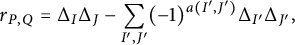 $$\begin{align*}r_{P,Q}=\Delta_I\Delta_J-\sum_{I',J'}(-1)^{a(I',J')}\Delta_{I'}\Delta_{J'},\end{align*}$$
where the sum is over
 $I',J'$
obtained from
$I',J'$
obtained from
 $I,J$
by swapping the last
$I,J$
by swapping the last
 $n-k$
entries
$n-k$
entries
 $\{a_{n-k},\ldots ,a_{n-1}\}$
of I with all possible choices of
$\{a_{n-k},\ldots ,a_{n-1}\}$
of I with all possible choices of
 $(n-k)$
-subsets of J, with
$(n-k)$
-subsets of J, with
 $\Delta _I=\sum _{K\in \mathcal {E}(I)}L_{K}$
and
$\Delta _I=\sum _{K\in \mathcal {E}(I)}L_{K}$
and
 $a(I',J')$
is the total number of swaps needed to put both
$a(I',J')$
is the total number of swaps needed to put both
 $I'$
and
$I'$
and
 $J'$
in order, defined above.
$J'$
in order, defined above.
Let
 $R=\{r_{P,Q}\:|\: P\succcurlyeq Q\text { noncomparable}\}$
be the set of all such relations.
$R=\{r_{P,Q}\:|\: P\succcurlyeq Q\text { noncomparable}\}$
be the set of all such relations.
Example 6.9. Let P be the blue Dyck path and Q be the black Dyck path in Figure 20 with
 $I=I(P)=\{1,2,5\}$
and
$I=I(P)=\{1,2,5\}$
and
 $J=I(Q)=\{1,3,4\}$
. Then the first index k such that
$J=I(Q)=\{1,3,4\}$
. Then the first index k such that
 $a_k> b_k$
is
$a_k> b_k$
is
 $k=3$
with
$k=3$
with
 $a_k=5>b_k=4$
. We have the relation
$a_k=5>b_k=4$
. We have the relation
 $$\begin{align*}r_{P,Q}=\sum_{\substack{\sigma\in \mathcal{E}(\{1,2,5\})\\ \kappa\in \mathcal{E}(\{1,3,4\})}}L_\sigma L_\kappa + \sum_{\substack{\sigma\in \mathcal{E}(\{1,2,3\})\\ \kappa\in \mathcal{E}(\{1,4,5\})}}L_\sigma L_\kappa -\sum_{\substack{\sigma\in \mathcal{E}(\{1,2,4\})\\ \kappa\in \mathcal{E}(\{1,3,5\})}}L_\sigma L_\kappa.\end{align*}$$

Figure 20: A pair of noncomparable Dyck paths.
The following key lemma is our “straightening algorithm.”
Lemma 6.10 For
 $P \succcurlyeq Q$
, the leading term of
$P \succcurlyeq Q$
, the leading term of
 $r_{P,Q}$
is
$r_{P,Q}$
is
 $L_QL_P$
.
$L_QL_P$
.
Proof Recall that the leading term is the smallest (in terms of Dyck paths) monomial, compared from large to small. By Lemma 6.8, the leading term of
 $\Delta _I$
is
$\Delta _I$
is
 $L_{P(I)}$
, if I is a Catalan subset. And for a pair of noncomparable Dyck paths
$L_{P(I)}$
, if I is a Catalan subset. And for a pair of noncomparable Dyck paths
 $P \succcurlyeq Q$
with
$P \succcurlyeq Q$
with
 $I=I(P)$
and
$I=I(P)$
and
 $J=I(Q)$
, the leading term of
$J=I(Q)$
, the leading term of
 $\Delta _I\Delta _J$
is
$\Delta _I\Delta _J$
is
 $L_QL_P$
.
$L_QL_P$
.
Keep the notations as in this section. Let’s examine the set
 $$\begin{align*}I'=\{a_1,\ldots,a_{k-1},b_{m_1},\ldots,b_{m_{n-k}}\}\end{align*}$$
obtained from I in the definition of
 $r_{P,Q}$
(Definition 6.2), where
$r_{P,Q}$
(Definition 6.2), where
 $m_1<\cdots <m_{n-k}$
. Without loss of generality, assume all elements in
$m_1<\cdots <m_{n-k}$
. Without loss of generality, assume all elements in
 $I'$
are different, as we have
$I'$
are different, as we have
 $\Delta _{I'}=0$
if otherwise. For each
$\Delta _{I'}=0$
if otherwise. For each
 $i=1,2,\ldots ,n-1$
, if
$i=1,2,\ldots ,n-1$
, if
 $i\leq k-1$
, we have
$i\leq k-1$
, we have
 $a_1,\ldots ,a_{i}\leq 2i$
; and if
$a_1,\ldots ,a_{i}\leq 2i$
; and if
 $i\geq k$
, we have
$i\geq k$
, we have
 $a_1,\ldots ,a_{k-1}\leq 2i$
, and at least
$a_1,\ldots ,a_{k-1}\leq 2i$
, and at least
 $i-k+1$
number of elements from
$i-k+1$
number of elements from
 $\{b_{m_1},\ldots ,b_{m_{n-k}}\}$
that are less than or equal to
$\{b_{m_1},\ldots ,b_{m_{n-k}}\}$
that are less than or equal to
 $2i$
since
$2i$
since
 $J=\{b_1<\cdots <b_{n-1}\}$
is a Catalan subset. This means that for each i, there are at least i elements from
$J=\{b_1<\cdots <b_{n-1}\}$
is a Catalan subset. This means that for each i, there are at least i elements from
 $I'$
that do not exceed
$I'$
that do not exceed
 $2i$
, and by Lemma 6.6,
$2i$
, and by Lemma 6.6,
 $I'$
is a Catalan subset. Moreover, by definition of k, the smallest number among
$I'$
is a Catalan subset. Moreover, by definition of k, the smallest number among
 $\{b_{m_1},\ldots ,b_{m_{n-k}}\}$
is at most
$\{b_{m_1},\ldots ,b_{m_{n-k}}\}$
is at most
 $b_k<a_k$
. Thus, the ith smallest number of
$b_k<a_k$
. Thus, the ith smallest number of
 $I'$
is smaller than or equal to the ith smallest number of I for
$I'$
is smaller than or equal to the ith smallest number of I for
 $i\leq k$
; and the kth smallest number of
$i\leq k$
; and the kth smallest number of
 $I'$
is strictly smaller than the kth smallest number of I. This is saying
$I'$
is strictly smaller than the kth smallest number of I. This is saying
 $P(I')\succcurlyeq P(I)=P$
and
$P(I')\succcurlyeq P(I)=P$
and
 $P(I')\neq P$
.
$P(I')\neq P$
.
For each term
 $L_{P'}L_{Q'}$
in
$L_{P'}L_{Q'}$
in
 $\Delta _{I'}\Delta _{J'}$
in the relation
$\Delta _{I'}\Delta _{J'}$
in the relation
 $r_{P,Q}$
, by Lemma 6.8 and the argument above,
$r_{P,Q}$
, by Lemma 6.8 and the argument above,
 $P'\succcurlyeq P(I')\succcurlyeq P\succcurlyeq Q$
and
$P'\succcurlyeq P(I')\succcurlyeq P\succcurlyeq Q$
and
 $P'\neq P$
. So the monomial
$P'\neq P$
. So the monomial
 $L_{P'}L_{Q'}$
(no matter which one of
$L_{P'}L_{Q'}$
(no matter which one of
 $P',Q'$
is larger) is strictly larger than
$P',Q'$
is larger) is strictly larger than
 $L_PL_Q$
in our term order. As a result,
$L_PL_Q$
in our term order. As a result,
 $L_PL_Q$
is the leading term of
$L_PL_Q$
is the leading term of
 $r_{P,Q}$
as desired, with coefficient
$r_{P,Q}$
as desired, with coefficient
 $1$
from
$1$
from
 $\Delta _I\Delta _J$
that cannot be canceled.
$\Delta _I\Delta _J$
that cannot be canceled.
Theorem 6.11 The set of relations R is a Gröbner basis of the ideal
 $\mathfrak {I}_n$
. The graded piece
$\mathfrak {I}_n$
. The graded piece
 $G_{n,d}$
of the grove algebra has a linear basis given by
$G_{n,d}$
of the grove algebra has a linear basis given by
 $\{L_{\mathbf {P}}\:|\: \mathbf {P}\in \mathcal {C}_n^{(d)}\}$
.
$\{L_{\mathbf {P}}\:|\: \mathbf {P}\in \mathcal {C}_n^{(d)}\}$
.
Proof We have
 $R\subset \mathfrak {I}_n$
by construction. To show that
$R\subset \mathfrak {I}_n$
by construction. To show that
 $\{L_{\mathbf {P}}\:|\: \mathbf {P}\in \mathcal {C}_n^{(d)}\}$
spans
$\{L_{\mathbf {P}}\:|\: \mathbf {P}\in \mathcal {C}_n^{(d)}\}$
spans
 $G_{n,d}$
, we use induction on the total order on the monomials. If a monomial
$G_{n,d}$
, we use induction on the total order on the monomials. If a monomial
 $L_{\mathbf {Q}}$
is not standard, where
$L_{\mathbf {Q}}$
is not standard, where
 $\mathbf {Q}=(Q_1\preccurlyeq \cdots \preccurlyeq Q_d)$
, then there exists some k such that
$\mathbf {Q}=(Q_1\preccurlyeq \cdots \preccurlyeq Q_d)$
, then there exists some k such that
 $Q_k\nleq Q_{k+1}$
. We now have a noncomparable pair of Dyck paths. Subtracting
$Q_k\nleq Q_{k+1}$
. We now have a noncomparable pair of Dyck paths. Subtracting
 $L_{\mathbf {Q}}$
by the relation
$L_{\mathbf {Q}}$
by the relation
 $r_{Q_{k+1},Q_k}\cdot L_{Q_1}\dots L_{Q_{k-1}}L_{Q_{k+2}}\dots L_{Q_d}$
, we obtain a polynomial whose leading term is greater than
$r_{Q_{k+1},Q_k}\cdot L_{Q_1}\dots L_{Q_{k-1}}L_{Q_{k+2}}\dots L_{Q_d}$
, we obtain a polynomial whose leading term is greater than
 $L_{\mathbf {Q}}$
. By the induction hypothesis, this difference can be written as a linear combination of
$L_{\mathbf {Q}}$
. By the induction hypothesis, this difference can be written as a linear combination of
 $\{L_{\mathbf {P}}\:|\: \mathbf {P}\in \mathcal {C}_n^{(d)}\}$
, so
$\{L_{\mathbf {P}}\:|\: \mathbf {P}\in \mathcal {C}_n^{(d)}\}$
, so
 $L_{\mathbf {Q}}$
can also be written as a linear combination of
$L_{\mathbf {Q}}$
can also be written as a linear combination of
 $\{L_{\mathbf {P}}\:|\: \mathbf {P}\in \mathcal {C}_n^{(d)}\}$
in
$\{L_{\mathbf {P}}\:|\: \mathbf {P}\in \mathcal {C}_n^{(d)}\}$
in
 $G_n$
. Thus, standard monomials span. By Proposition 6.4 on the dimensions, we conclude that the standard monomials form a basis of
$G_n$
. Thus, standard monomials span. By Proposition 6.4 on the dimensions, we conclude that the standard monomials form a basis of
 $G_n$
. Moreover, this means that R generates the ideal
$G_n$
. Moreover, this means that R generates the ideal
 $\mathfrak {I}_n$
, since any additional relation reduces the dimension of some graded component
$\mathfrak {I}_n$
, since any additional relation reduces the dimension of some graded component
 $G_{n,d}$
.
$G_{n,d}$
.
To see that R is in fact a Gröbner basis of
 $\mathfrak {I}_n$
, we need to show that the leading terms of polynomials in R, which are
$\mathfrak {I}_n$
, we need to show that the leading terms of polynomials in R, which are
 $\{L_PL_Q\:|\: P,Q\text { are noncomparable}\}$
, generate the initial ideal
$\{L_PL_Q\:|\: P,Q\text { are noncomparable}\}$
, generate the initial ideal
 $\mathrm {init}_{\preccurlyeq }(\mathfrak {I}_n)$
. In other words, it suffices to show that for any
$\mathrm {init}_{\preccurlyeq }(\mathfrak {I}_n)$
. In other words, it suffices to show that for any
 $f\in \mathfrak {I}_n$
, the leading term of f is not standard. Assume the opposite that the leading term of f is
$f\in \mathfrak {I}_n$
, the leading term of f is not standard. Assume the opposite that the leading term of f is
 $L_{\mathbf {Q}}$
with coefficient
$L_{\mathbf {Q}}$
with coefficient
 $1$
, where
$1$
, where
 $\mathbf {Q}=(Q_1\leq \cdots \leq Q_d)$
. As explained in the previous paragraph, for any other monomial
$\mathbf {Q}=(Q_1\leq \cdots \leq Q_d)$
. As explained in the previous paragraph, for any other monomial
 $L_{\mathbf {Q}'}$
in f, we can write it as a linear combination of standard monomials which are weakly greater than
$L_{\mathbf {Q}'}$
in f, we can write it as a linear combination of standard monomials which are weakly greater than
 $\mathbf {Q}'$
, thus strictly greater than
$\mathbf {Q}'$
, thus strictly greater than
 $\mathbf {Q}$
. Applying this procedure, we obtain a nonzero relation on the standard monomials, contradicting that standard monomials form a basis.
$\mathbf {Q}$
. Applying this procedure, we obtain a nonzero relation on the standard monomials, contradicting that standard monomials form a basis.


 Open access