

Details
Section 1 provides an introduction with a motivation for the use of stochastic full balance sheet model.
Section 2 describes the use of firm’s regulatory and economic capital models, how these interact and their key constituent elements.
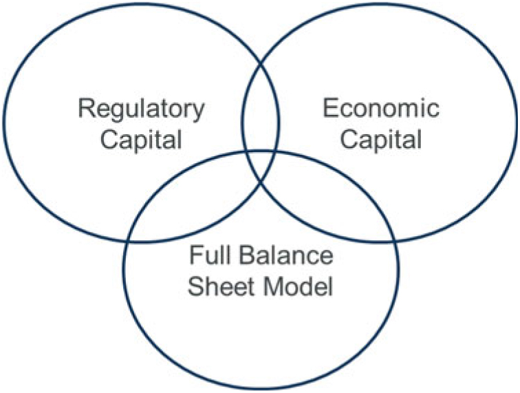
Section 3 sets out an overview of a full balance sheet model including its interaction and overlap with regulatory and economic capital models.
Section 4 sets out an example model based on annuity liabilities that will be used throughout the paper to demonstrate the techniques discussed.
Section 5 provides an introduction to proxy modelling and importantly, the roll forward techniques used to re-base proxy functions. The annuity example specified in section 4 is used to demonstrate a simple proxy-fitting process.
Section 6 shows how a proxy model can be derived to model changes in a firm’s solvency capital requirement (SCR). Techniques are demonstrated that may be used under either a variance covariance or copula simulation approach.
Section 7 demonstrates techniques that may be used to derive a proxy function to the risk margin (RM) and discusses an approach that may be used for transitional measures.
Section 8 brings together the example fits for the net assets, SCR and RM and uses these to show the risk exposure in the complete example model.
Section 9 discusses the challenges of realistically modelling changes to the discount rates applicable to VA, MA and pension scheme business.
Section 10 shows how the proxy model derived may be used to generate risk appetite 1-in-X metrics and ruin probabilities.
Section 11 focuses on the identification of ruin events and demonstrates how the focus on actual events such as this may be more useful for risk management purposes than standard capital allocation techniques. Within this section, techniques are demonstrated that can be used to derive the most likely ruin event.
Section 12 discusses the roll forward and projections of the proxy models in order that the model can remain current and also be used to understand how the stability of the balance sheet position is forecast to evolve over future years.
Section 13 concludes the paper with a summary of the key points that have been discussed and finally looks at the limitations of the model.
This paper is written with a focus on UK life insurance firms under the Solvency II regime. A number of the techniques discussed within are likely to be applicable in a wider context.
This paper is intended for UK or European Life actuaries who are interested in:
• Risk management
• Risk appetite
• Proxy modelling
• Own risk and solvency assessment (ORSA)
It is expected that the reader will have a working knowledge of the key aspects of Solvency II.
Disclaimer
The views expressed in this paper are those of the author and not necessarily those of the IFoA. The IFoA do not endorse any of the views stated, nor any claims or representations made in this paper and accept no responsibility or liability to any person for loss or damage suffered as a consequence of their placing reliance upon any view, claim or representation made in this paper.
The information and expressions of opinion contained in this paper are not intended to be a comprehensive study, nor to provide actuarial advice or advice of any nature and should not be treated as a substitute for specific advice concerning individual situations.
1. Introduction
1.1 Purpose
1.1.1 This section contains an introduction and a discussion of the main motivation for the use of a stochastic full balance sheet model.
1.2 Definition
1.2.1 For the purposes of this paper, a stochastic full balance sheet model is defined to be a stochastic model that describes changes in the full Solvency II balance sheet of an insurer.
1.3 Motivation for the model
1.3.1 A fundamental element of the risk management of an insurer relates to understanding the firm’s regulatory capital position as measured by its Solvency II surplus. A firm needs to ensure it has sufficient surplus currently and over future years so as to be able to meet its business objectives and its obligations to policyholders. It is important to be able to understand not just the strength of the capital position but also how stable the position is and the nature of the risks that affect it.
1.3.2 In recent years, there has been an increasing focus in the insurance industry on the use of risk appetite frameworks. The purpose of these frameworks is to enable firms to be able to understand the amount and types of risk that a firm is willing to assume in order to meet its business objectives. Risk appetite frameworks typically encompass a number of different elements such as earnings, liquidity and reputation. Perhaps the most important element is the capital risk appetite.
1.3.3 The capital risk appetite refers to the risk that a firm’s regulatory capital position may be insufficiently strong to meet its objectives. Firms typically hold a capital “buffer” in excess of the minimum amount of required regulatory capital as a defence against this risk. One approach that may be used to assess the amount of a buffer required is to apply stress tests to the balance sheet. An alternative approach is to stochastically model changes in the capital position over a 1-year time frame and therefore be able to quantify the probability of regulatory insolvency as a 1-in-X year amount.
1.3.4 In May 2018, the PRA released supervisory statement SS4/18 regarding financing planning and management by insurers. The statement sets out the PRA’s expectations regarding firm’s use of risk appetite statements including that:
“The insurer’s risk appetite statement is expected to include the risk appetite for the levels of capital that are to be maintained in reasonably foreseeable market conditions (e.g. as assessed through stress and scenario tests, or through some suitable alternative approach, to provide no more than a 1-in-X probability that Solvency Capital Requirement (SCR) coverage might fall below 100%)’’.
The statement also discusses the importance of allowing for non-linearity associated with combinations of adverse events and the use of reverse stress testing.
1.3.5 SS4/18 discusses that firms should take into account balance sheet sensitivity to key risk drivers and discusses how firms should understand their balance sheet volatility. In modelling such measures, it is important to take into account changes in the full balance sheet including elements such as the SCR and RM in addition to allowing for changes in the value of assets and liabilities. This draws a distinction between firm’s SCR capital models and a stochastic full balance sheet model that may be used for risk appetite purposes.
1.3.6 In addition to allowing for changes in SCR and RM, there may be other important areas of difference between a firm’s SCR model and a stochastic full balance sheet model. An example is the use of the volatility adjustment (VA). The UK regulator does not permit the SCR calculations to allow for changes in the value of the VA under credit stresses.Footnote 1 In practice, the VA will actually vary under credit stresses according to a predetermined formula. Therefore for a stochastic full balance sheet model to be realistic, it must take into account changes in the VA (including how this affects the liabilities and also the SCR).
1.3.7 In summary, a stochastic full balance sheet model provides the means by which firms can understand the nature of risks to their regulatory balance sheet. This has always been an important element of effective risk management but has taken on increasing importance more recently due to the focus within the industry on the use of risk appetite frameworks.
2. Types of group model
2.1 Purpose
2.1.1 Solvency II Pillar 1 uses a Value at Risk (VaR) framework over a 1-year time horizon. Under the Solvency II regime, firms typically have two main types of group model, the regulatory capital model and the economic capital model. This section discusses the nature of these models, their key components and their interactions.
2.2. Overview
2.2.1 A firm’s regulatory capital model is used to calculate its SCR and RM. These must be calculated either through the SII standard formula (SF) or through a firm’s internal model (IM) subject to regulatory approval. The purpose of the regulatory capital model is to calculate the amount of SCR and RM required to be held by the regulator. Where a firm uses the SF, the SCR and RM are calculated as per the formula prescribed in the SII delegated regulations. Where a firm uses an IM, a firm has its own model of its risks and exposures and uses a formula set out in its own documentation to calculate the SCR and RM.
2.2.2 A firm’s economic capital model is normally used in its ORSA. The model is used to form a firm’s own view of the capital required to meet its liabilities (which may be similar or different to its regulatory capital). The model may be used in any assessment of the appropriateness of the SF for a firm. The model would be expected to be used in business decision making.
2.2.3 A group model has the following main components:Footnote 2
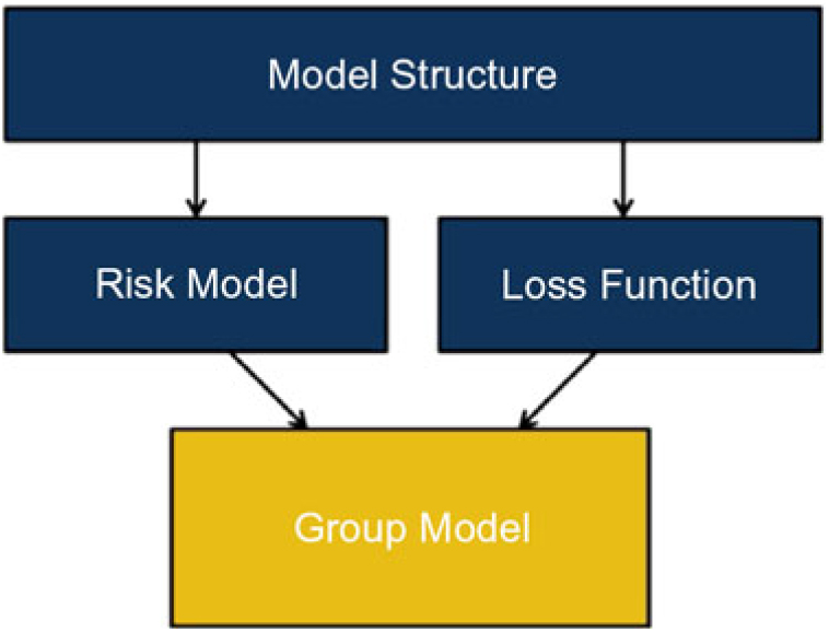
2.2.4 The model structure consists of the form of the model. The structure includes
• The risk measure (e.g. VaR over 1 year at the 99.5th percentile)
• The risks included in the model
• The elements we are calculating losses over (e.g. the assets and liabilities)
The model structure would be expected to remain stable over time other than for changes such as an emerging risk or a new product line.
2.2.5 For a 1-year VaR framework, the risk model represents our view of the joint probability distribution of the risk movements over the 1-year time frame. It therefore takes into account the marginal distribution of each risk and the way risks interact to form the joint distribution.
2.2.6 The loss function is a function that expresses changes in value (e.g. a firm’s net assets for an SCR model or firm’s balance sheet for a full balance sheet model), as a function of movements in the risks included in the structure. The loss function represents the “true” changes in value as a function of risk movements as calculated using full runs of a firm’s asset and liability models. A “proxy model” or “proxy function” is an approximation to the loss function. Proxy models are described in detail in section 5.
2.2.7 Loss functions may be used to describe changes in value at different business levels. For example, they may be used at the level of individual assets or product liabilities, or instead used for losses at an aggregate level (e.g. for a business unit or at a group level). A loss function at an aggregate level is composed of the sum of individual loss functions within, together with any allowance for effects such as tax or fungibility that can be calculated only at an aggregate level.
2.3 Regulatory Capital Model (SII IM)
2.3.1 Where a firm uses a SII IM, the model structure in this case is mostly specified by regulation. Elements that are prescribed in regulations include, for example, that:
• the SCR is calculated using a 1-year VaR approach at the 99.5th percentileFootnote 3
• firms may use a matching adjustment (MA) or VA according to specified rules
• The calculation of the RM is based on projected non-hedgeable risk SCRs, allowing for a 6% cost of capital charge
2.3.2 Other elements of a firm’s IM give greater freedom for the model structure. For example, the risks used are selected and defined by the firm.
2.3.3 For their risk model, the majority of IM firms use a copula (Embrechts et al., Reference Embrechts, Lindskog and McNeil2001; Shaw et al., Reference Shaw, Smith and Spivak2010) simulation approach. In this case the risk model is precisely specified by the risk distributions used and the copula.Footnote 4 The risk model is specified by each firm. However, there has been a significant convergence of risk calibrations and methodology within the industry as firms strive to remain in line with the market. As a result of this, there is a risk that firm’s IM calibrations represent a general market calibration rather than their true view.
2.3.4 A smaller number of IM firms use a traditional variance covariance formula rather than a copula simulation approach. Such an approach does not in itself imply the use of a particular risk modelFootnote 5 (i.e. we cannot infer what the joint risk distribution used is). For this reason, it may be appropriate for such firms to specify first the type of risk model they are assuming. Once specified, firms may then note that they are using a variance covariance formula to calculate their capital requirements under this model.
2.3.5 The loss function under IM represents changes in the values of net assets as a function of changes to the IM risks. Under a copula simulation approach, proxy functions are normally used to estimate the value of changes.Footnote 6
2.3.6 Where firms use a variance covariance formula, this formula is applicable where losses are a linear function of each risk with no allowance for cross terms (i.e. the cost of an event of two risks is the sum of the cost on each risk). The linear function is calibrated based on individual 1-in-200 stresses.
2.3.7 Firms that use a variance covariance formula may recognise the limitations of the formula and use a non-linearity adjustment (normally based on a single equivalent scenario technique). Under such an approach, the loss function in the model reflects the full movements in assets and liabilities, with the formula giving an approximation to these full movements.
2.4 Regulatory capital model (SII SF)
2.4.1 The SF is often thought of as being based on the use of normal distributions. However, the risk model (if any) used in the SF has never actually been articulated. The SF uses a variance covariance formula approach with a modular structure. Such an approach isn’t consistent with any form of risk distribution or loss function. Footnote 7 For this reason, the SF should be regarded as a formula for calculating a firm’s SCR and RM rather than a true group model.
2.4.2 Although the risk model has not been articulated, the calculations used in the SF are almost fully specified in the SII delegated regulations.Footnote 8 However, there are elements of the structure that are specified by individual firms. For example, firms may choose (subject to regulatory approval) to use the VA on part of their business. The detailed calculations required for liabilities valuation are also chosen by firms.
2.5 Economic capital model
2.5.1 The model structure to be used in an EC model is not prescribed in regulation and is therefore free to be determined by each firm. In practice, the model structure may be closely aligned with firm’s regulatory capital models (e.g. they are likely to use a 1-year VaR measure). There may also be important differences such as the inclusion of the RM or the percentile used to calculate VaR.
2.5.2 The risk model used in an EC model is typically closely related to that used in the regulatory capital model for IM firms. However, there may be differences in the risk model used (risk calibrations and correlations) as firms look to use fully realistic calibration in their EC. SF firms may include their own risk model to form their internal view of risks.
2.5.3 The loss function used in a firm’s EC model would typically be the same as for a firm’s IM regulatory capital model, other than where model structure differences exist (e.g. if a firm used a dynamic VA in EC but static VA in IM). SF firms may include their own loss function to form their internal views.
3. Design of the stochastic full balance sheet model
3.1 Purpose
3.1.1 Within this section, the stochastic full balance sheet model is described in detail.
3.2 Overview
3.2.1 Of the models described earlier, the purpose of the regulatory capital model is to determine the level of SCR and RM to be held for regulatory purposes. These are the amounts required by the regulator to ensure policyholders have the appropriate level of protection.
3.2.2 The economic capital model by contrast represents a firm’s own view of the amounts required to give appropriate protection to policyholders. Where the economic capital results exceed regulatory capital results, firms would normally ensure they have sufficient capital to meet the higher amount.
3.2.3 Both the regulatory capital model and the economic capital model are concerned with the protection of policyholders. What neither of these are designed to do is to model the stability of the solvency position of a firm and to therefore ensure that it has sufficient regulatory surplus to meet its business objectives. This is the purpose of a stochastic full balance sheet model.
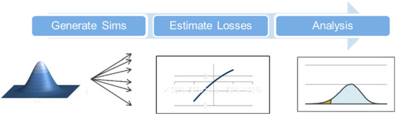
3.2.4 In practice, a stochastic full balance sheet model is a model in which stochastic real-world simulations are generated and, within the simulations, losses to the regulatory balance sheet surplus are estimated. The resulting simulations may be used for a variety of purposes including the calculation of 1-in-X buffer amounts for risk appetite purposes or finding the probability of ruin.Footnote 9
3.2.5 The stochastic full balance sheet model is intended to be a fully realistic assessment of how the regulatory balance sheet behaves. As such the model may be closely aligned to an EC or regulatory capital model in some areas. For other areas, there may be important differences. For example, for a book of annuities that use the VA, we may have:
• A regulatory capital model required to use a static VA
• An economic capital model that uses an illiquidity premium different to the VA
• The stochastic full balance sheet model which must realistically model the regulatory capital position
In order to realistically model the regulatory capital position, in this case, means that we need to consider the effects on the net assets, SCR and RM.
3.2.6 For the net assets, the best estimate liability (BEL) is affected by changes in the VA in response to market spreads. Therefore we need to incorporate a dynamic VA.
3.2.7 For the SCR, SCR calculations are based on the difference between the BEL and the BEL under stress events. As the BEL is affected by the VA, the SCR will also be affected by the VA (even though the stress calculations within that SCR are based on a static VA).
3.2.8 The RM is calculated without VA so the RM is unaffected.
3.2.9 In summary, the design of the stochastic full balance sheet model is likely to include elements of the design of both the regulatory capital and economic capital models. The degree of alignment to these models is determined by a balance between the need to include bespoke functionality for full balance sheet modelling against the desire to have alignment between models for reasons of cost and maintenance.Footnote 10
3.2.10 It is important to be clear on the distinction between a stochastic full balance sheet model and a true economic capital model. An economic capital model is intended to represent the true economic value of a firm’s assets and liabilities. In contrast, a stochastic full balance sheet model is intended to be used to understand how the regulatory requirements (the assets, BEL, SCR and RM) for the firm change under stress.
3.3 Stochastic full balance sheet model – Model structure
3.3.1 The structure of a stochastic full balance sheet model comprises elements such as the time frame, risk measure, risks included and the elements modelled (e.g. assets, liabilities, SCR, RM).
3.3.2 For practical reasons, models would be expected to use the 1-year VaR framework normally used in firms’ regulatory and economic capital models. The use of a 1-year VaR framework is also the metric required to provide 1-in-X year ruin event probabilities as set out in the PRA supervisory statement SS4/18. The use of a short time frame such as this means the model may not be suitable for understanding longer-term risks such as an economic downturn over many years.
3.3.3 Firms’ regulatory capital models use the 99.5th percentile as specified under the SII regulations. A firm’s economic capital may use a different percentile or indeed the results at a number of different percentiles. Typically, results from a stochastic full balance sheet model would be required at a variety of different percentiles depending on the purpose.
3.3.4 The risks included in the model should be those that are realistically expected to have a material effect on the firm’s solvency position. The risks would normally be the same as those included in a firm’s economic model. It should also be noted that there are some risks that cannot be practically incorporated in a firm’s model. Examples of these are set out in section 13.
3.3.5 The elements modelled need to include the components of the SII regulatory balance materially affected by the modelled risks. These elements include assets and liabilities, together with the SCR and RM. Further elements such as transitional measures may also be included. A key consideration in the design is to set the level of model granularity used appropriately. A detailed model comprised of a high number of individual proxy functions has a higher maintenance cost and run time than a simpler model but may give a more detailed insight into a firm’s risk exposure.
3.4 Stochastic full balance sheet model – Risk model
3.4.1 Within a stochastic full balance sheet model, a key element is the risk model. Typically UK insurers use a copula simulation model.Footnote 11 The elements required to parameterise the risk model are the distribution of each risk, together with the copula. To fully specify the risk model, it is necessary to specify the type of copula and the copula parameters (e.g. the correlation matrix).
3.4.2 A firm’s economic model represents the firm’s best view of the true nature of the risks it is faced with. For this reason, the risk model would normally be aligned with the economic model. One key question is whether the risk model should be at a Point in Time (PIT) or Through the Cycle (TTC).
3.4.3 A PIT model is calibrated to reflect conditions at the current time. For example, a PIT equity model may take into account current levels of market volatility. A TTC model is calibrated to reflect more general conditions over an extended period of time. For this reason, the calibration of a TTC model is stable over time (other than small changes to represent new data) whereas a PIT model calibrations may vary significantly. In practice, any model has an element of PIT calibration as the model will reflect the conditions in the data period for which it has been calibrated over.
3.4.4 Firms’ IM regulatory capital models are normally TTC. The key reason for this is that using PIT models for regulatory capital throughout the industry could lead to significant problems with pro-cyclicality. Economic capital models are also normally TTC as firms wish to maintain consistency with their IM models and maintain a stable level of EC.
3.4.5 For SF firms, no true risk model has been specified as set out earlier. However, the formula includes a symmetric adjustment mechanism to equity stresses that is equivalent to a change in risk model dependent on recent conditions. The symmetric adjustment mechanism’s purpose is to provide an element of anti-cyclicality rather than to represent a true PIT model.
3.4.6 For a stochastic full balance sheet model, a TTC calibration would normally be used as this has the benefits of giving alignment with firms’ (IM) regulatory capital and EC models.Footnote 12 A key output to the model may be a required level of risk buffer to be held for risk appetite purposes against the risk of regulatory insolvency. Using a PIT model for this purpose would give rise to a risk of pro-cyclicality in the industry for similar reasons as in firms’ regulatory capital models.
3.4.7 Whereas TTC calibrations may be considered the most suitable for calculating a risk appetite buffer, a PIT calibration is most suitable for firm’s realistic decision making, for example, where firms wish to estimate their true ruin probability over the coming year for risk management purposes. This can be estimated much more accurately using a PIT model.
3.4.8 In summary, a stochastic full balance sheet model would normally be calibrated with a TTC calibration to give alignment with its regulatory and economic models and for use in risk appetite calculations. However, it should be recognised and effectively communicated that the use of a TTC calibration in 1-year ruin probability calculation has limitations.
3.5 Stochastic full balance sheet model – Loss function
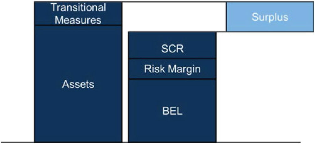
3.5.1 The overall loss function in a stochastic full balance sheet model needs to take into account changes in the value of net assets, SCR and RM. It may also take into account transitional measures on technical provisions (TMTP) if required. It is helpful to consider the SII balance sheet is in the following form.
3.5.2 The granularity of proxy models used is an important part of the model design. The granularity of assets and liabilities used in a stochastic full balance sheet model would normally be the same as used under a firms SCR model for practical purposes.
3.5.3 The proxy models used to represent changes in the value of assets would normally be the same as used under an IM SCR model.
3.5.4 The proxy models used to represent changes in the value of liabilities may need to be recalibrated compared to those used in IM SCR calculations to ensure they reflect realistic movements in the value of these under different risk events. A key example here is business for which the VA is used. The VA is not permitted to be changed under stress in the UK, whereas in practice it moves in response to credit spread changes. For this reason a separate calibration is required for use in a stochastic full balance sheet model. Section 9 gives further detail.
3.5.5 To model changes in the SCR, RM and TMTP, it is necessary to calibrate proxy functions that estimate how the value of these items realistically may change under stress events. As for other proxy functions, this typically consists of the use of a set of runs used to calibrate the model with a further set of runs used to test the fit performance. Sections 6 and 7 give further detail.
4. Example model
4.1 Purpose
4.1.1 In order to demonstrate the techniques discussed in this paper, an example model will be used as specified in this section. The example model uses a simple annuity book to demonstrate the techniques that may then be applied to more complex company models.
4.1.2 Different approaches are required depending on whether a firm uses an IM or the SF. For completeness, both these approaches will be covered in the example.
4.2 Liabilities
4.2.1 The example book contains 100,000 identical annuitants with the following features:
• Annuity amount – £1,000 p.a. paid annually in arrears, no escalation
• Age – 60
• Expenses, £100 p.a. increasing with RPI
4.2.2 Mortality assumptions
• Mortality rates are as per an example table set out in Appendix B.
4.2.3 Economic assumptions
• Yields 2% at all durations
• RPI 1.5% at all durations
4.2.4 Discount rates
The base version of the example assumes the annuities are discounted using the yield curve only. However, an allowance for a VA is introduced in section 9. The VA takes a base value of 0.18%.
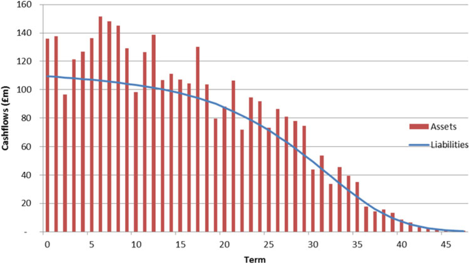
4.3 Assets
4.3.1 The annuities are assumed to be backed by risk-free fixed interest cash flows (e.g. using gilts) with a pattern that broadly covers the run-off of the liabilities. The asset cash flows have a small excess over the expected liability run-off at most terms. The following graph shows the pattern of assets compared to the liabilities:
4.4 Model structure
4.4.1 A single period model using a 1-year time frame is used. The model includes the following risks:
• Longevity L – applied by multiplying the assumed mortality rates by (1+L)
• Expense E – applied by multiplying the assumed expenses by (1+E)
• Inflation I – applied as an addition to RPI at all terms
• Credit Cr – applied as an increase to all spreads of Cr
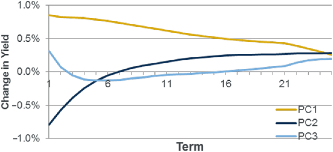
The model also includes an allowance for interest rate risk. In common with many UK firms, interest rate risk is modelled through the use of principal components analysis (PCA; Abdi and Williams Reference Abdi and Williams(2010))Footnote 13 to describe changes in the yield curve.
4.4.2 The PCA eigenvalues and eigenvectors used in the example model are set out in Appendix C. The model structure applies a vector change to the spot yield curve defined as
 $$\left[ {Change\,in\,Yield} \right] = 0.01A{\sqrt {Eval1}} \,\,\left[ {EVec1} \right] + 0.01B{\sqrt {Eval2}} \,\left[ {EVec2} \right]\, + 0.01C{\sqrt {Eval3}}\, \left[ {EVec3} \right]$$
Where A, B, C are the risk coefficients for PC1, PC2, PC3
Eval1, Eval2, Eval3 are the eigenvalues set out in Appendix C
Evec1, Evec2, Evec3 are the eigenvectors set out in Appendix C
The shape of the principal components can be seen in the following graph:
4.4.3 The elements the loss function applies to are the changes in net assets (the assets and liabilities defined earlier), changes in SCR and changes in RM.
4.4.4 The RM is calculated as the projected value of future non-market risks, allowing for a 6% cost of capital charge as prescribed in the SII regulations. A risk driver approach is used to estimate the future longevity and expense risk. The future longevity risk is estimated using the BEL as a risk driver. The future expense risk is estimated using the BEL in respect of expenses only as a driver.Footnote 14
4.5 Risk model
4.5.1 The risk model is that the risks have a joint normal distribution. The distribution is specified through marginal risk distributions combined using a Gaussian copula. The marginal risk distributions are specified as follows:
Longevity L ∼ N(0,7.76%) (1-in-200 is 20%)
Expense E ∼ N(0,19.41%) (1-in-200 is 50%)
Inflation I ∼ N(0,0.78%) (1-in-200 is 2%)
Credit Cr ∼ N(0,1.55%) (1-in-200 is 4%)
PC1 A ∼ N(0,100%)
PC2 B ∼ N(0,100%)
PC3 C ∼ N(0,100%)
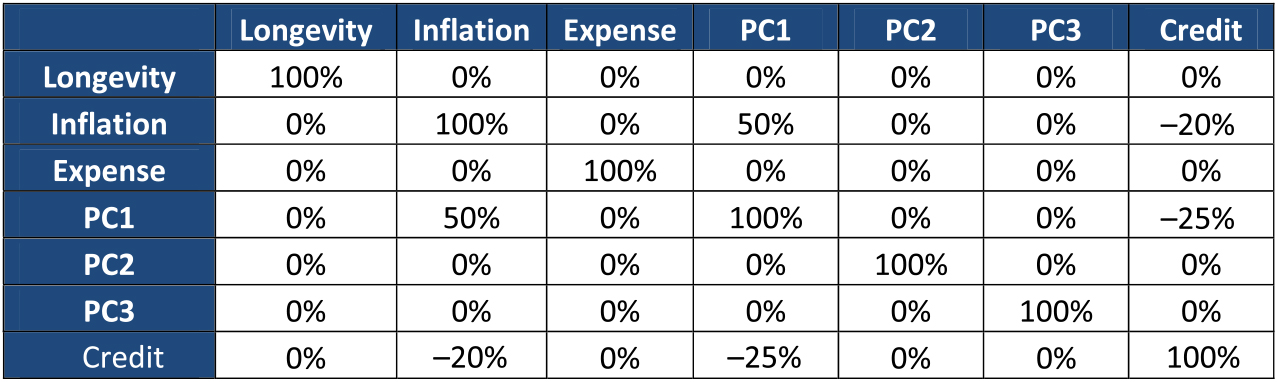
The correlation matrix used in the Gaussian copula is as follows:
4.6 Loss function
4.6.1 The loss function in the model is the sum of individual loss functions on the net assets (simply the assets and liabilities set out earlier), the SCR and the RM. In sections 6 and 7, the SCR and RM will be calculated as per the SII SF. Section 6 also shows an example of how to allow for an IM SCR calculated using a copula simulation approach.
4.7 Starting surplus
4.7.1 It is assumed that the model firm has a regulatory surplus on its SII balance sheet of £250m.
4.8 Risk appetite
4.8.1 It is assumed that the model firm has a risk appetite framework whereby it plans to be able to have a surplus buffer sufficient to withstand a 1-in-30 shock over a 1-year time horizon. A fall below a 1-in-10 level triggers urgent corrective action.

5. Proxy models
5.1 Purpose
5.1.1 The purpose of this section is to give a high-level introduction to the use of proxy modelling in group stochastic models (such as those used in many firm’s IM SCR calculations). The section gives details of how such models may be calibrated and validated, together with how a roll forward process may be used to allow for how the models may change in response to events.
5.2 Overview
5.2.1 Group stochastic models in the UK typically use a copula simulation approach over a 1-year time frame. A copula approach is normally used as this allows firms to specify a probability distribution for each risk, together with the copula which is then used to combine these to form the joint risk distribution. Within the models, a high volume of real-world simulations (e.g. one million) are generated according to a specified copula and marginal risk distributions. Within the output, it is then necessary to estimate the changes in the value of the firm’s net assets in each of the simulations. The results of this are used to form the probability distribution of net assets which may be used to derive results such as the 99.5th percentile VaR.
5.2.2 Within a group stochastic model, it will therefore be necessary to estimate changes to the value of assets and liabilities under a large number of different risk events, each of which consists of changes to parameters for each risk in the model. Given unlimited time and resources, this could be achieved by running the firm’s full asset and liability models. Of course this cannot be practically achieved. Therefore proxy models are used to provide an approximation to the results that may be obtained from the full models. In practice, the key uses of proxy models are within IM firms’ Solvency II SCR calculations (including the use of these models for business decision making).
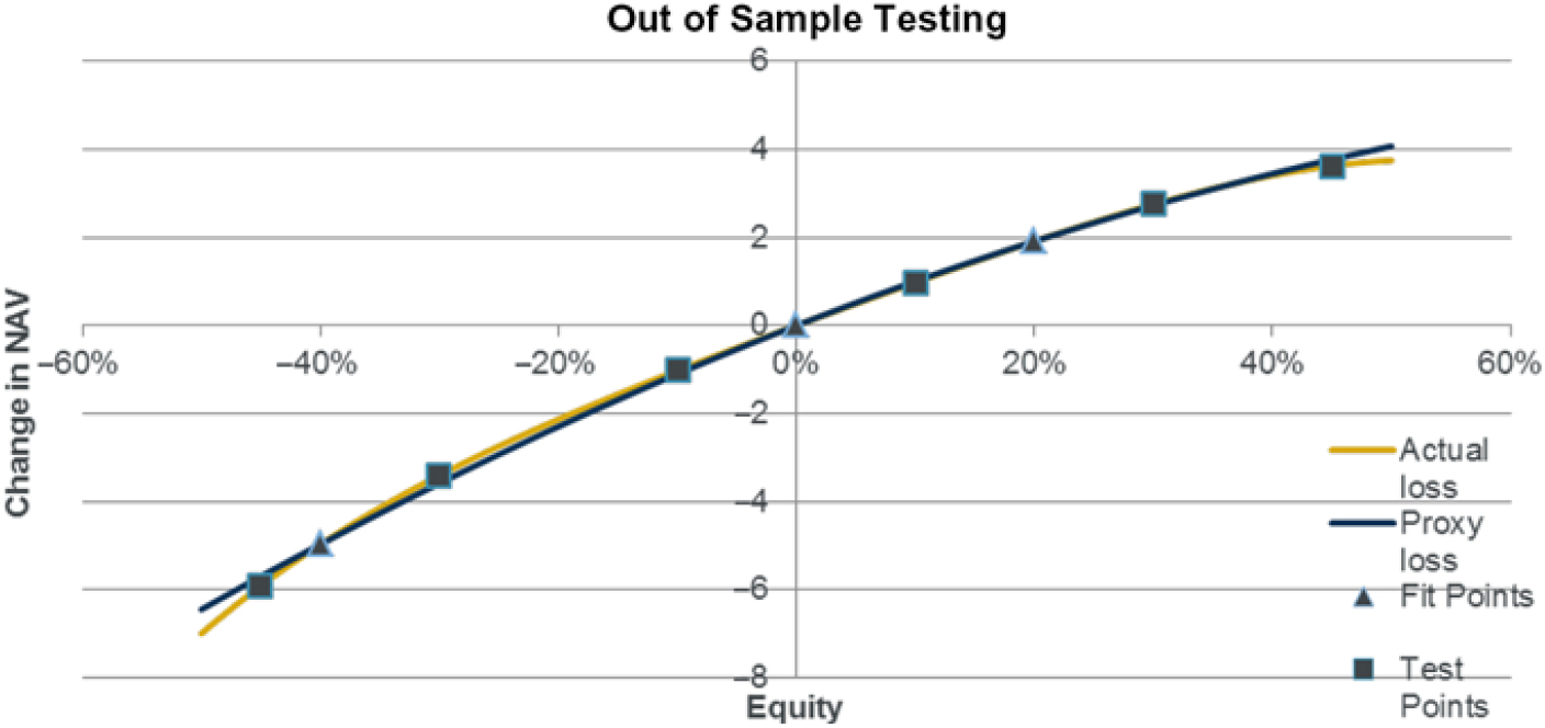
5.2.3 A proxy model used in group risk modelling is a function that approximates the changes in net assets as a function of the risk movements included in the model. The following example shows a proxy function in a single risk. In practice the net assets are exposed to a number of risks.
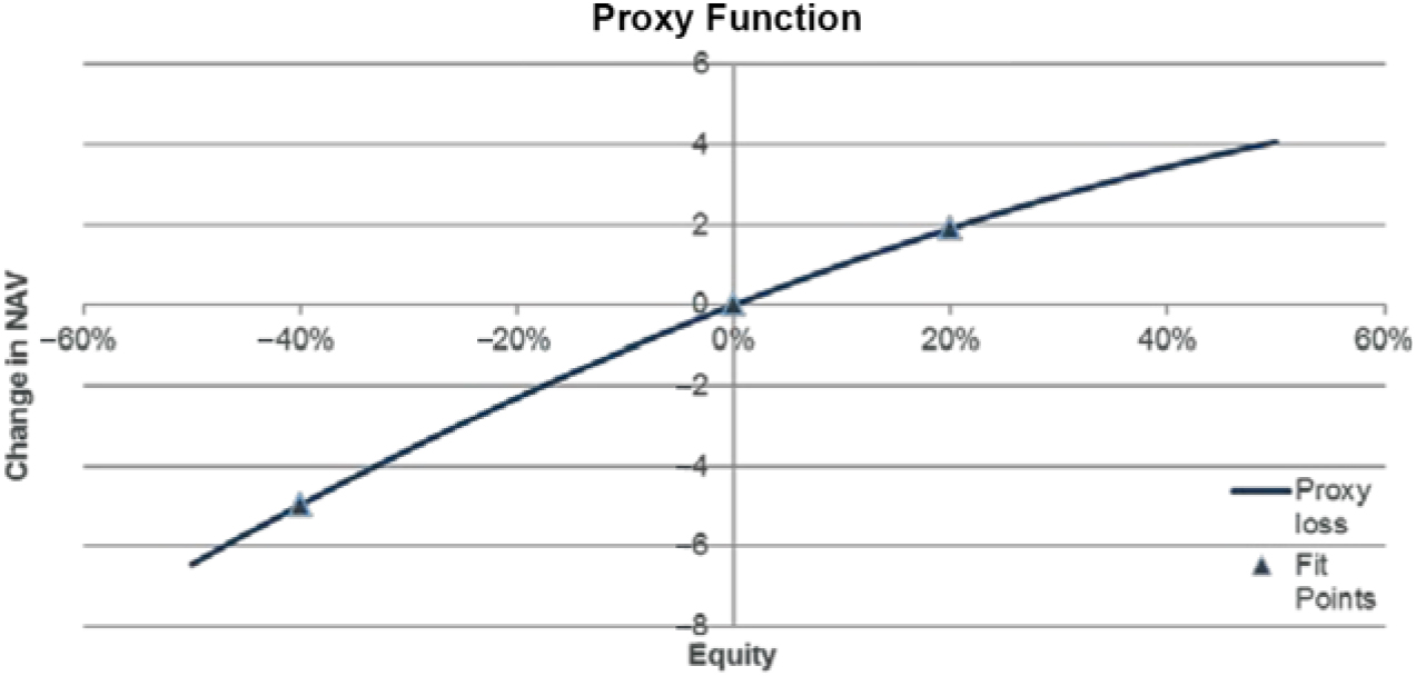
5.2.4 A proxy model may take a number of different forms. The most common approach is to approximate changes in net assets through a polynomial function of the risks. The polynomial would include terms for individual risks as well as “cross terms” to allow for the interaction between two or more risks.
5.2.5 A proxy model often takes the form of a sum of individual proxy functions (applied to particular assets and liabilities). There may be exceptions for features such as tax, fungibility or management actions that need to be applied at portfolio level, on particular portfolios of assets and liabilities.
5.2.6 A key requirement for a proxy function is that it must be able to be rapidly executed in order that it be evaluated a large number of times in a group stochastic model. Before a proxy model can be used, a process of calibration and then validation must be carried out.
5.3 Calibration set
5.3.1 Calibration of a proxy model requires the use of a set of runs to parameterise the model. The calibration set should give a suitable coverage of the range of different values each risk may take. It is important that the proxy model performs accurately in a range of scenarios. For example moderate stresses may be important for solvency monitoring, extreme stresses for capital calculations and reverse stress testing.
5.3.2 An important part of model calibration is the specification of the calibration set. This may be done through judgement, taking into account the materiality of each risk and the extent to which we may expect cross terms (e.g. we normally expect interactions between longevity risk and interest rate risks).
5.3.3 An alternative technique commonly used to specify fitting runs is to use a Sobol Reference Sobol(1967) sequence. The Sobol sequence is used to efficiently partition the risk space used for the calibration to ensure the fitting runs give a good coverage of all risk combinations. A Sobol sequence is generally a lot quicker to use where specifying a large number of calibration runs. It would normally be expected to give a stronger performance than using judgment-based runs, but this is not always the case as it does not for example take into account the materiality of each risk.
5.4 Model selection
5.4.1 Model selection is the process by which the form of model is selected (e.g. the maximum order of polynomial used for individual and combined risks). Once the form of model is selected, the model parameters can then be fitted (typically by a least squares regression). The model selection process may typically be carried out by identifying the most appropriate polynomial form up to a given maximum order. If a good fit cannot be achieved, alternative models may be considered. The process is typically repeated over each of the individual proxy functions to be calibrated.
5.4.2 A simple approach to model selection is to produce graphs and other analysis to determine the model to be used. For example, if graphs showed losses plotted against longevity were close to a straight line then a proxy function with a linear longevity term would be used.
5.4.3 A key objective in the model selection process is to ensure the model uses only the terms necessary to achieve a good fit and no more. The “in sample fit” (the least squares result over the calibration set) can almost always be improved through using more terms. However, the use of an excessive number of terms can lead to problems with “overfitting” whereby the model fit in the calibration set is very close but performance outside this set is poor (see validation later).
5.4.4 A more sophisticated approach is to use a model selection algorithm (Efroymson, Reference Efroymson, Ralston and Wilf1960). A number of such algorithms are available which provide a sequential approach to automatically select the variable terms to be included in the model. Perhaps the most commonly used approach is a stepwise regression. The approach is designed to include terms within the model provided their inclusion is statistically significant.
5.5 Validation
5.5.1 The purpose of proxy model validation is to be able to assess the performance of the proxy models as measured by how closely they reproduce the underlying full model results.
5.5.2 The strongest approach to proxy model validation is to use an out of sample (OOS) test set of runs. The accuracy of the proxy model over the test set can be assessed using a range of statistics such as the average error and average squared error.
5.5.3 Firms may use a variety of different approaches to derive the OOS test set to be used. It is important that such approaches take into account combined risk events rather than just individual risks and give appropriate focus to all areas for which the model may be used. For example, if the OOS runs are focused only on fit performance in the kind of scenarios that give 99.5th percentile losses, then they may be untested on the more moderate kind of events used for purposes such as roll forwards or stress testing.
5.5.4 A useful approach to OOS testing is to use randomly generated simulations from the group risk model so that overall expected error statistics can be calculated. Similarly, simulations close to the 99.5th percentile losses can be used to estimate the expected error in the SCR.
5.5.5 It is important that the OOS testing is truly independent of the selection process. For example, if different step regression algorithms are used and the one giving the best OOS results is selected, this means the OOS set is now part of the calibration process and cannot be used to give an independent performance assessment.
5.6 Roll forwards overview
5.6.1 Proxy model calibration is an intensive process that may take place, for example, once or twice a year (different individual elements of the overall proxy function may be calibrated at different times). Roll forward is the process by which a model calibrated to a particular date is rolled forward to give an up-to-date model.
5.6.2 A roll forward process would be expected to take into account changes in the loss function (as represented by a proxy function) and the risk model. Changes to the proxy function need to reflect the updated balance sheet response to risk movements. Changes to the risk model would be used, for example, to take into account a change in an equity risk distribution that has taken place since the calibration date.Footnote 15
5.6.3 A roll forward process would normally take into account features such as the run-off of business, risk movements (e.g. economic changes) and new business. Within the roll forward process, actual movements experienced in the above items are allowed for.
5.6.4 A projection process is very similar to a roll forwards process. The key difference is that projection assumptions are used rather than actual movements. Where projections are carried out over a long time frame (e.g. several years), it is important to consider the limitations of proxy modelling for this purpose. Section 12 gives further details.
5.6.5 There are a number of different techniques that may be used to approximate the effects of the above features; for example, expected run-off could use a simple scaling factor for each loss function to reflect expected business run-off, or instead a more sophisticated approach could be used to reflect the changing risk characteristics of the business as it runs off.
5.6.6 In order to model 1-in-X type movements in the SII balance sheet, a key focus is on the ability to model changes in SCR and RM under different risk movements. Risk movements are equivalent to economic variances, demographic variances and basis changes in the above list.Footnote 16
5.7 Roll forwards risk movements
5.7.1 Under a roll forward process, for risk movements, the first task is to map economic and demographic variances, together with basis changes onto values of the coefficients for each risk. As an example, within a model containing a single equity risk (rather than different risks to represent different equity markets), over the roll forward period, different equity markets will have different returns. A weighted average of these returns can be used to derive a representative equity risk movement for the period.Footnote 17 For a 1-year period, the movement represents an observation from the equity risk distribution.
5.7.2 For basis changes, these can be mapped to a value of each risk movement precisely in some cases but approximately for others. In the annuity example above, a 5% reduction in the probability of death at all ages simply corresponds to a longevity risk movement of −5%. If, for example, a change in mortality was only applied beyond age 70, this does not directly correspond to the definition of the risk. An approximate risk movement can be found through approximations such as solving for the risk movement that corresponds to the change in BEL that has occurred.
5.7.3 Demographic variances are unlikely to have a material impact on the group model results under normal circumstances (e.g. a month of higher than normal mortality has little impact on the group balance sheet aside from any accompanying basis change). An exception may be in the event of a mass lapse or mortality catastrophe event. Should these have occurred a risk movement can normally be derived from the percentage of policyholders affected.
5.8 Roll forwards update of proxy function
5.8.1 A key part of the roll forward process is to be able to model the manner in which a proxy function changes following a risk movement. As an example, a proxy function would be expected to show greater exposure to longevity risk following an interest rate fall due to the decreased amount of discounting.
5.8.2 Provided the proxy function has been appropriately calibrated,Footnote 18 it can be used to derive a re-based proxy function that shows the new changes in net assets as a function of the risk movements.
5.8.3 The approach used to derive re-based proxy functions depends on the definition of each risk. There are two main ways in which a risk can be defined: an additive risk or a multiplicative risk. An example of an additive risk is the credit risk model specified in section 4. In this model, spreads are calculated as the current spread, plus Cr - the credit risk value. An example of a multiplicative risk is longevity in the example model. The probability of death at age x = q x (1 + L) where L is the longevity risk value.
5.8.4 As an example of how a re-based proxy function is derived for an additive risk, consider a proxy function including just interest rates (as a flat stress). In this example, the proxy function is specified as follows:Footnote 19
 $${\rm f}( x ) = x - 20 \times 2$$
Consider a 1.6% change in interest rates. This is equivalent to redrawing the axes of the graph at the 1.6% point.

to give:

5.8.5 Mathematically, the new re-based proxy function f’(x) can be expressed as
f’(x) = f(x + a) – f(a) where a is the movement amount (1.6% in this example).
The subtracted term f(a) is required here as proxy functions represent the change in NAV compared to the current position. The current position is equal to the base position with the addition of f(a).
In this example
 \[\begin{array}{*{20}{l}} {f(x)}&{ = x - 20{x^2}{\mkern 1mu} {\rm{we}}\,{\mkern 1mu} {\rm{have}}}\\{f(x)}&{ = {\rm{f}}(x + a) - f(a)}\\{}&{ = (x + a) - 20{{(x + a)}^2} - (a - 20a2)}\\{}&{ = (x + a) - 20{x^2} - 40ax - 20{a^2} - a + 20a2}\\{}&{ = (1 - 40a)x - 20x2}\\{}&{{\rm{For}}\:a\:{\rm{is}}\:1.6\% {\mkern 1mu} {\rm{we}}\:{\rm{have}}\:f'\:(x) = 0.36x - 20x2}\end{array}\]
5.8.6 For multiplicative risks, in addition to the effects shown for additive risks of moving around the loss function, there is also the multiplicative element to the risk movement that needs to be taken into account. As an example, we may model expense risk as a multiplicative risk such that the expense following a stress is:
IE (1 + E) where IE is the initial expense amount per policy, E is the expense stress.
An example proxy function is:
change in NAV = −rE r is a constant
Under an extreme example, if E is −100%, then we no longer have any expenses and so the rebased proxy function is zero. On the other hand if E is 100%, expenses have doubled and so any further expense risk movements also have doubled the effect due to the multiplicative nature of the risk.
The rebased proxy function is:
Change in NAV = −2rX
5.8.7 In general, for multiplicative risks, the rebased loss function is specified as:
 $${\rm f'}(x) = {\rm f}( {( {1 + a})x + a}) - {\rm f}( a )$$
In the above expense example, where expenses double and so a is 1 the rebased loss function is
 \[\begin{array}{*{20}{l}}{{\rm{f'}}(x)}&{ = {\rm{f}}((1 + a)x + a) - {\rm{f}}(a)}\\{}&{ = {\rm{f}}((1 + 1)X + 1) - {\rm{f}}(1)}\\{}&{ = {\rm{f}}(2X + 1) - {\rm{f}}(1)}\\{}&{ = - r(2X + 1) + r.1}\\{}&{ = - 2rX - r + r}\\{}&{ = - 2rX}\end{array}\]

5.8.8 The above examples have considered proxy functions in a single risk only. In general, a proxy function for a number of risks may have a combination of additive and multiplicative risks. In this case the rebased function takes the additive or multiplicative form for each risk.
e.g. for risks x additive and y multiplicative, with movements a and b respectively, the rebased loss function is specified as:
$${\rm f'}( {x,y} ) = {\rm f}( {x + a\,( {1 + b} )y + b} ) -{\rm f}( {a,\!b})$$

5.8.9 One final type of risk that requires a different approach is catastrophe type risks typically modelled through a frequency and severity model. Examples of these risks are operational risk and general insurance catastrophe risks. For these risks, normally no changes in the proxy function would normally be allowed for in response to risk movements.
5.8.10 The cost of an operational risk event may actually depend on other risks (e.g. interest rates if the operational risk event has a long-term cost). These effects should in theory be taken account of through a proxy function that allows for operational risk losses as a function of different risks and can therefore be used in the roll forward process. However, firms’ operational risk models are unlikely to fully allow for this level of detail.
5.9 Proxy model example – Calibration
5.9.1 Using the annuity model specified above, it can be demonstrated how a simple proxy function can be calibrated to the net assets. In this example, the process has used:
• A calibration set consisting of 1,023 runsFootnote 20 according to a Sobol sequence on the modelled risks
• A candidate set of terms consisting of all individual and combined risk terms up to order 4 polynomials
• A stepwise regression algorithm is used with p value 5%
• No VA assumed
For the calibration runs, the assets and liabilities have been revalued and a proxy function fitted to the results.
5.10 Proxy model example – Validation
5.10.1 Validation of the model has been carried out using a test set of 100 OOS points drawn at random from the joint probability distribution. A comparison of the predicted versus actual results is shown below:

The graph (supported by error statisticsFootnote 21) shows a very close fit, and so the proxy model has been accepted.
5.11 Proxy model example – Key exposures
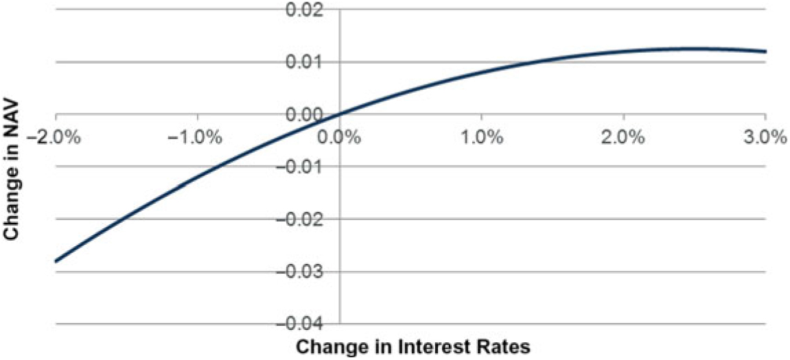
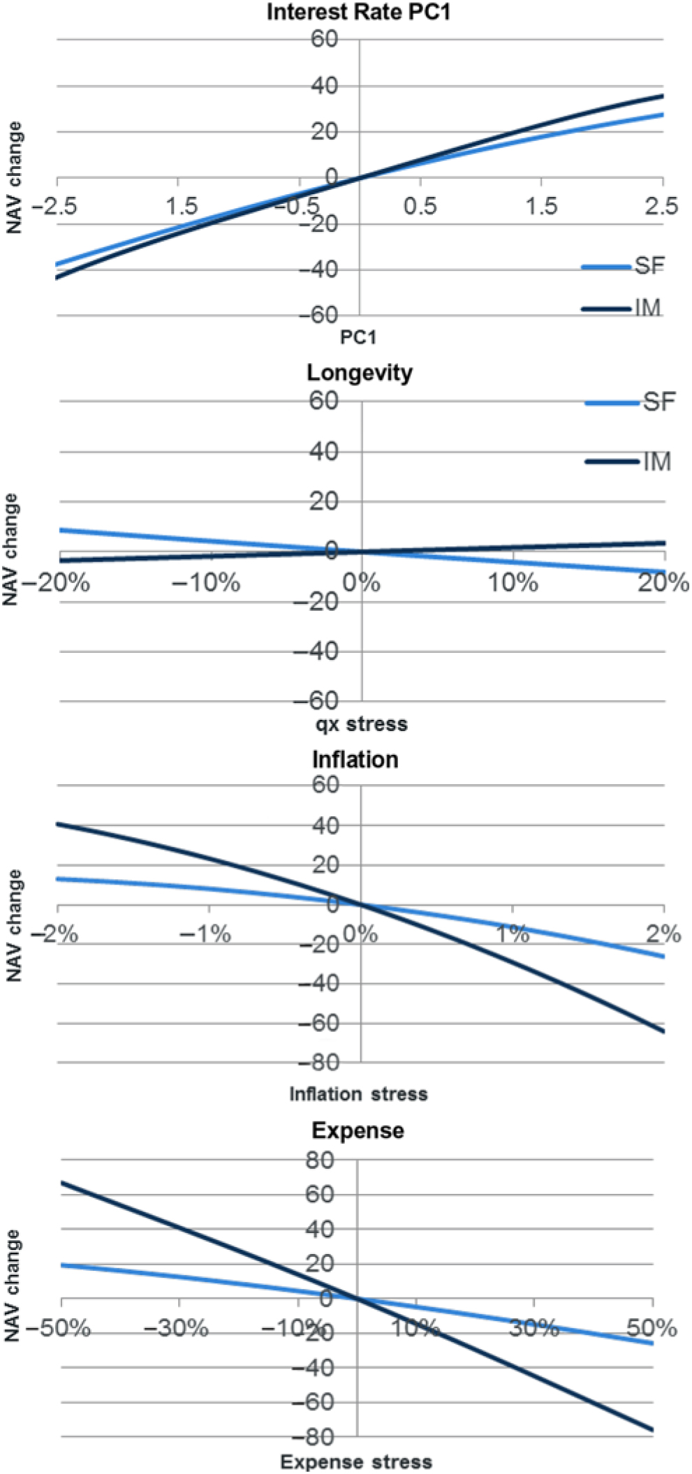
5.11.1 The key risk exposures in the model can be seen in the following graphs:

5.11.2 The results show, as expected, that the annuity book is exposed to increases in expenses, inflation and life expectancy (falling q x). The interest rate exposure is to increasing yields (PC1 broadly reflects an increase in the level of the curve). The reason for this directional exposure is that there is a small excess of assets over liabilities which gives a cost as interest rates rise. This result is specific to the example being used. More generally the direction of interest rate exposure of an annuity book depends on the matching position of the assets used to back the liabilities.
5.12 Proxy model example –Joint risk exposures
5.12.1 Whereas individual risk exposures can be easily graphed as above, to visualise the effects of two risks at a time requires 3d or contour-style graphs. The following graph shows the combined exposure to interest rate PC1 and longevity (represented by q x changes). Of course there are important exposures to many other risk combinations.

5.12.2 In this plot, the proxy function is represented by the shaded areas, the boundaries of which represent combinations of PC1 and q x that give a constant loss. The threat direction arrows are perpendicular to the lines of constant loss and are used to show the direction of increasing losses.
5.12.3 The graph shows exposure to rising interest rates and falling q x as shown in the individual graphs. The graph also shows a change in the threat direction close to the bottom of the graph. This shows that under a significant reduction in q x, the interest rate exposure actually goes from an exposure to increases in yield to a more neutral exposure. This reflects a change from a position of excess assets to liabilities to a closer match following a large longevity event. It should be noted that this effect is specific to the example given and that the nature of the exposures depends on the specific details of the assets and liabilities.
6. SCR proxy fitting
6.1 Purpose
6.1.1 Within this section, the complexities of fitting proxy functions to allow for changes in SCR are discussed. In order to calibrate proxy functions for changes in SCR, the approach to be used is different depending on whether a firm uses a variance covariance formula method (as is used in the SF) or copula simulation approach.
6.2 SCR fitting –Variance covariance formula – Overview
6.2.1 As with all types of proxy model fitting, fitting to the SCR is carried out by initially evaluating changes to the SCR under a calibration set. Once complete a proxy function can be fitted to the results and validation can be carried out using standard approaches as described above. In practice, this may mean several hundred revaluations of the SCR under different stresses. As the SCR itself may be made up of multiple stresses (approximately 25 stresses for the SF), to fully revalue the SCR several hundred times is likely to be impractical.
6.2.2 In order to be able to practically revalue the SCR several hundred times, an approach that may be used is to use the existing proxy model and roll forward process. The key to achieve this is to be able to estimate the 1-in-200 stress results for each risk in the SCR using the proxy model. The roll forward process then may be used to estimate how the 1-in-200 results change following stress events.
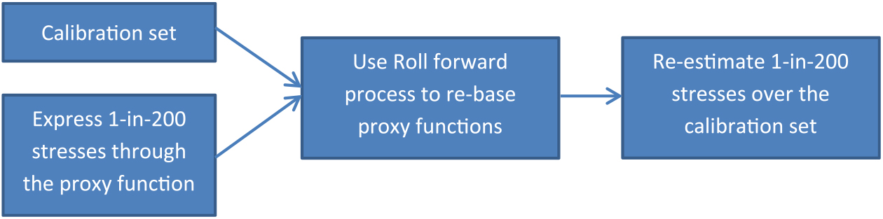
6.2.3 Where there is alignment between the risk definitions used in the proxy model and those used under the SCR, this may be relatively simple; however, where differences arise, an alternative approach may be required.
6.2.4 One further point of consideration here is whether there are any changes in the risk model following a stress. Section 2 discusses whether the SF could be considered to have a true risk model. Notwithstanding this point, the equity stress used under the SF contains a symmetric adjustment mechanism in which the stress varies depending on recent equity returns. This is equivalent to a change in the risk model following a stress.
6.2.5 In addition to considering the equity stress, a further point of discussion in the SF is the interest rate stresses. These are specified as multiplicative factors to apply to different points on the spot curve. The interest rate-up stresses are subject to a minimum level of 1%. No stresses are applied where rates are negative. This specification means that the interest rate element of the risk model differs depending on the level of the curve. Therefore, the SF risk model changes following an interest rate stress.
6.2.6 Under a more general variance covariance formula approach, any features such as those discussed above under the SF will need to be taken into account where material.
6.2.7 The approach used to revalue the SCR under stress would be expected to vary depending on the nature of the business and model. To illustrate some of the techniques that may be used, a proxy function will be used to calibrate to the annuity model above. The firm is assumed to calculate its capital requirements using the SII SF.
6.3 SCR fitting – Variance covariance formula SF example
6.3.1 Within the annuity model, exposure exists to longevity, expenses, inflation and interest rates. Under the SII SF, inflation risk is not separately captured and so no stress calculation is required. The approach used for longevity, expense and interest rates is discussed below.
6.3.2 Under the SF, the longevity risk 1-in-200 event is specified as a 20% fall in qx. This event definition is in line with the model structure set out in section 4 above. Therefore, the cost of a longevity 1-in-200 stress may be found by using a value of −20% in the proxy function.
If we specify the proxy function as f(L, I, E, Cr, A, B, C) where the terms represent the risks as defined in section 4 (A, B, C represent interest rates PC1, PC2, PC3), we may calculate the 1-in-200 longevity capital as −f(−20%, 0, 0, 0, 0, 0, 0).

6.3.3 The SF expense stress is made up of an increase to the level of expenses of 10%, together with a 1% increase in expense inflation. The SF stress is therefore not consistent with the model structure used in the example model. However, the SF stress can be simply calculated by applying an expense stress of 10% and an inflation stress of 1% in the loss function. The expense capital amount is therefore equal to –f(0, 1%, 10%, 0, 0, 0, 0).
6.3.4 The SF interest rate stresses consist of an up and down stress, specified as multiplicative changes to the spot yield curve subject to at least 1% (for the up stresses). No changes are applied for negative rates. The form of the SF stresses is therefore substantially different from that used in the example proxy model. The key differences are as follows:
• Specified up and down stresses (in vector form) are used rather than principal components.
• Multiplicative changes are used rather than additive.
• A floor of 1% is applied on the up stresses.
• The levels of the stresses are different.
6.3.5 Despite these differences, it is still practical to be able to estimate the SF stresses using the existing proxy model. The steps to do so are as follows:
1. Using the current yield curve, derive the SF stress curves (allowing for the 1% floor) and compare against the base curve to get the yield curve stress specified as an additive (vector) change.
2. Express the vector change as a linear combination of the proxy model principal components. Therefore derive the interest rate PC combination equivalent to each of the SF up and down stresses.
6.3.6 With regards to the second of these steps, PCA is used to break down changes in a yield curve (or other measure) so that rather than modelling individual points on the curve, the changes can be expressed in terms of its principal components (representing the main shapes of the changes). Therefore, using PCA we can approximate any yield curve movement as a linear combination of the PCs.
As an example, using the example model (with PC values shown in Appendix B), the following approximation to the SF yield down stress under a 2% base yield can be constructed:

The SF yield down capital (for 2% yield) may therefore be estimated as:
 $$-{\rm f}(0,\!0,\!0,\!0, - 1.23,\!0.25, - 1.16).$$
It should be noted that this process will be required for each of the calibration run stresses as the SF yield stresses vary as the yield curve changes.
6.3.7 Once the capital amounts for the longevity, expense and interest rate stresses have been derived, the SF capital amount may be derived using the SF aggregation formula.
6.4 SCR fitting – Variance covariance formula SF example results
6.4.1 Using the same calibration parameters as used in the net assets example in section 4, the following calibration graph can be obtained.
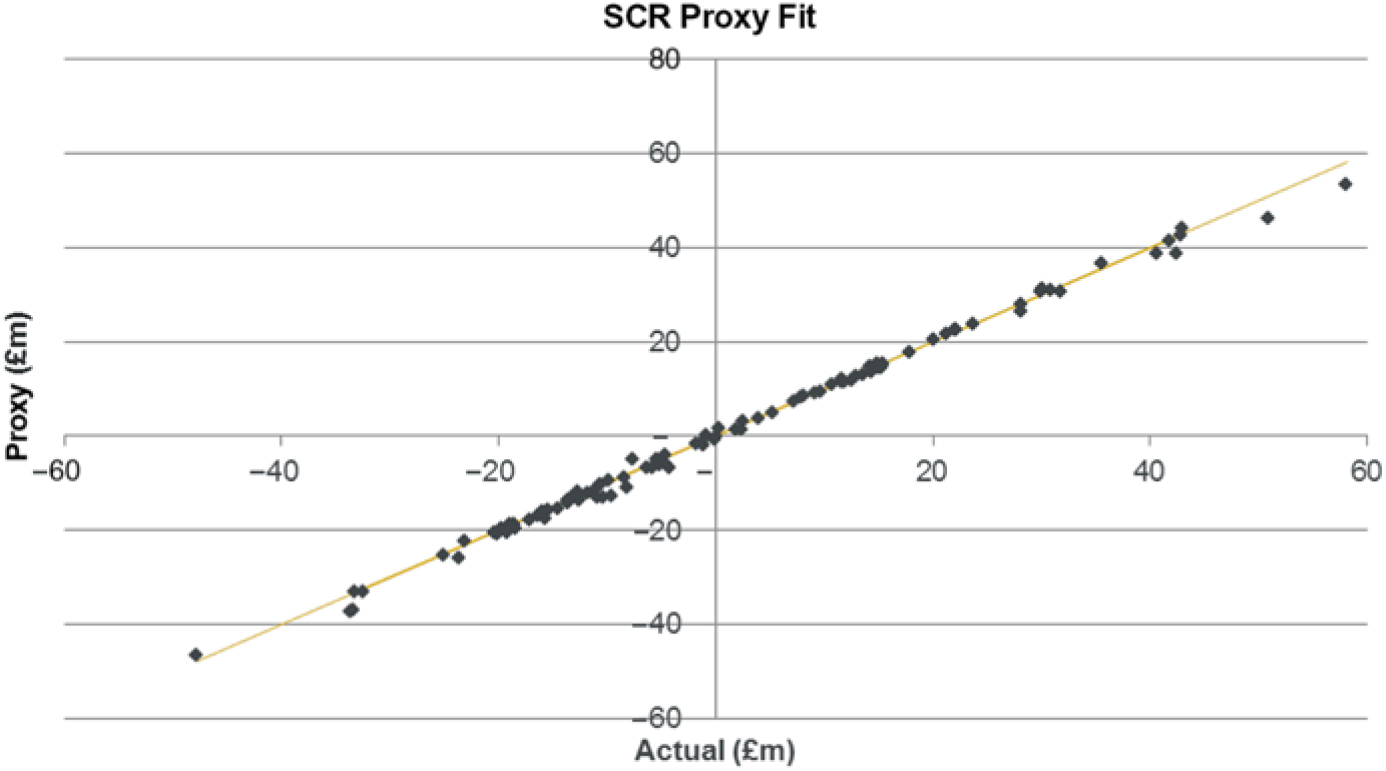
6.4.2 Note, in this case, that there are two levels of proxy modelling, the proxy fitting used to derive the net assets (assets and annuity liabilities) exposure, followed by the use of this proxy function to estimate the SF SCR. It is important in this case that the “actual” values in the above graph are derived from a full revaluation of the SCR under stress rather than being taken from the SCR estimated from the proxy function.
6.4.3 The above graph (and accompanying analysis) shows that the SCR proxy fit is suitably accurate. The OOS analysis above has been completed using 100 test points. In practice it may be necessary to use far fewer points for practical reasons.
6.5 SCR fitting – Variance covariance formula SF example – Key exposures
6.5.1 The following graphs show the key risk exposures for the SF SCR example. Here the graphs show how the SCR element of the overall surplus changes in response to risk movements (the graphs show the effect on the NAV).

6.5.2 As may be expected, the results show the SCR increases under increased inflation and expenses. This is simply that these increase the value of the expense element in the model, therefore increasing the cost of stresses.
6.5.3 The exposure of the SCR to interest rates is down (the opposite to the exposure of the net assets). The key reason for the exposure is that as interest rates fall, all the cash flows used in the calculations are discounted at a lower rate leading to an increase in the SCR. For this reason, it is very common for the SCR to be exposed to falling interest rates.
6.5.4 The exposure to longevity is unusual in that the exposure of the SCR is to increasing q x. Normally it may be expected that falling q x gives rise to greater annuity liabilities and therefore a greater SCR. However, due to the nature of the asset and liability position in the specified example, the fall in q x actually lead to a closer matching position between assets and liabilities. This has the effect that the interest rate capital in the SF SCR is reduced.
6.5.5 The analysis demonstrates how a proxy function can be fitted to give the estimated change in the value of the SCR. The results show that the effect can be material and the exposure may not be as expected.
6.6 SCR fitting – Copula simulation example
6.6.1 The above example demonstrated how a proxy function may be fitted to the SCR under a variance covariance approach as is used under the SF. Within this section, an approach that may be used for an SCR calculated by copula simulation model is discussed.
6.6.2 In practice, where a company uses a copula simulation model to calculate its IM SCR, there is likely to be close alignment between the risk model structure used in the regulatory capital model for SCR and the risk model structure used in an EC model and used in a stochastic full balance sheet model. This would mean the risks used and their definitions are the same (the calibrations could be different).
6.6.3 In most cases, in addition to alignment between the risk model structures used between the regulatory capital and stochastic full balance sheet models, there would normally be alignment between the loss function used for assets and liabilities in the different models. For example, under a 1% fall in yields, the cost to net assets this gives in the SCR model would be expected to be fully realistic. Therefore, that same cost would apply to the regulatory capital and stochastic full balance sheet models.
6.6.4 There are circumstances for which the loss function used in a stochastic full balance sheet model would be expected to differ from those used in the regulatory capital model. A key example to this is the use of the VA. The VA is not permitted to move under stress in the UK, whereas it does actually move in response to credit stresses. As the stochastic full balance sheet model is intended to model fully realistic changes in the balance sheet, it must take into account that the VA changes under stress, but the SCR calculations are on the basis of a static VA. Complexities around the use of the VA are discussed in further detail in section 9.
6.6.5 On the assumption that the risk model structure and the loss function are the same as in the regulatory capital model, the roll forward process may be used to adjust the proxy functions under each stress. The process may be carried out as follows:

6.6.6 Of course, the SCR model may be time-consuming to run, and so there may be practical difficulties with running a large calibration set. An approach that may be used to mitigate this is to run the SCR model with a reduced number of simulations. It may be helpful to use a different random seed for each run in order that any simulation error is spread across the different runs.
6.7 SCR fitting – Copula simulation example results
6.7.1 Using the annuity model example above, the assumption is now made that the SII SCR will be calculated using a copula simulation model over 10,000 simulationsFootnote 22 with the risk model and calibrations as set out in section 4 above. No VA is assumed.
6.7.2 A calibration set of 255 Sobol runs has been used rather than 1,023 as used previously (a smaller number is used to take into account the time required to carry out SCR runs). Other than this, the same approach to fitting as previously has been used. The fit performance results are set out below:

The fit performance has been considered to be suitably accurate.
6.8 SCR fitting – Copula simulation example – Key exposures
6.8.1 The following graphs show the key risk exposures. For comparison, the results are shown against the equivalent SF results set out above.
6.8.2 The IM results show a greater exposure to expense and inflation risk than for the SF. This reflects the fact that the expense and inflation risks (1-in-200s are 50% and 2%, respectively) included in the copula-simulated SCR have a stronger calibration than the expense stress used in the SF (expense risk has a 10% expense level increase and 1% increase to expense inflation). Of course, the SF stress applies the expense level and inflation stresses together, whereas in the copula simulation model diversification between the risks is allowed for.
6.8.3 Longevity risk in the copula-simulated SCR is of the opposite exposure to under the SF SCR. The copula-based exposure is as would be normally expected (policyholders living longer give greater BEL and so higher SCR). The reasons for the SF SCR exposure being in the opposite direction are set out in section 6.5 above. Much of the reason for the difference in direction is due to the SF SCR in this case being heavily influenced by the interest rate up 1-in-200 shock, whereas the copula simulation approach allows for interest rate exposure over all parts in the distribution.
6.8.4 Interest rate exposure is similar between the two sets of results. The slightly higher exposure in the IM copula simulation SCR reflects the SCR itself being slightly higher.
6.8.5 This example shows there may be significant differences in exposure depending on whether an SCR is calculated using a variance covariance approach such as that used in the SF or a copula simulation approach (as typically used in an IM). Of course, the nature of the differences depends on the respective calibrations used within the example model, and so this example should not be used to infer conclusions on the merits of an IM or SF approach.
7. RM and TMTP proxy fitting
7.1 Purpose
7.1.1 The purpose of this section is to discuss the challenges inherent in calibrating a proxy function to represent changes in a firm’s RM and TMTP. An example is used to demonstrate how this may be done for a firm using a variance covariance formula approach (in this case the SF). The same techniques are applicable for firms using copula simulation approaches.
7.2 RM overview
7.2.1 The RM is calculated by projecting future SCRs in respect of non-hedgeable risks, before applying a 6% p.a. cost of capital charge and discounting the results back to the valuation date at the risk-free rate. The most common approach used by firms to allow for future SCRs is a risk driver technique in which risk drivers such as the BEL or sum at risk are used to project the 1-in-200 risk capitals for each product and (non-hedgeable) risk used in the calculation.
7.2.2 Therefore, in order to fit a proxy function to the RM, the approach used is equivalent to that used for an SCR; however, some key differences must be taken into account:
• The RM calculation takes into account non-hedgeable risks only
• Changes in the risk free discount rate under stress need to be allowed for
• Changes in the run-off of risks (assuming a driver approach is used)
• The RM is calculated assuming no MA or VA is included
7.2.3 The exclusion of hedgeable risks from the calculation can be easily carried out. The modelling challenges concerning the MA and VA are discussed in detail in section 9 below. This section is therefore concerned with allowance for the changes in risk-free rate and run-off.
7.2.4 The allowance for changes in the risk-free rate used in the RM calculation is relatively simple. It can be carried out by applying the interest rate risk model over the base curve being used.
7.2.5 The allowance for changes in risk drivers may have a significant effect on the results. A key example is where a longevity event takes place in an annuity book. This has the effect that the run-off of future SCRs is slower leading to a higher RM. There are a number of different techniques that may be used to allow for changes in the run-off rate. For example, an approximation factor could be calculated so as to spread the run-off over a greater (or fewer) number of years for material risks.
7.2.6 The most simple and accurate approach to allow for run-off is simply to recalculate the drivers under each of the calibration runs. This may lead to a large number of runs, but these may actually be readily available. For example, using the annuity model, the calibration of the proxy function to assets and liabilities provides 1,023 runs from which the run-off of the BEL and other drivers may be obtained. Using these same 1,023 runs in the RM proxy calibration means the run-offs have already been produced.
7.2.7 Perhaps the most important exposure of the RM is to falling interest rates. These tend to have a compounding effect as the effects of falling interest rates normally increase the level of SCR (as seen in section 6) and, of course, reduce the discounting of the future SCRs. There may also be a smaller effect on the risk drivers’ run-off.
7.3 RM fitting SF annuity example
7.3.1 Using the annuity example SF model (without VA) above, the following approach has been used to calculate the RM.
1. Calculate the SF SCR in respect of the expense and longevity risks only (to represent the non-hedgeable risk).
2. The RM (as set out in section 4 above) is determined by projecting the longevity risk SCR using the BEL as a driver and the expense risk SCR using the BEL in respect of the expense cash flows only.
3. The RM is then calculated using the standard SII approach of discounting the future SCRs allowing for a 6% cost of capital charge.
7.3.2 In order to calculate an RM proxy function, the allowance for the change in risk drivers under stress is required. For this purpose, the actual run-off of the drivers has been used as described above. The following graph shows examples of the extent to which the run-off rate is affected by stress events:
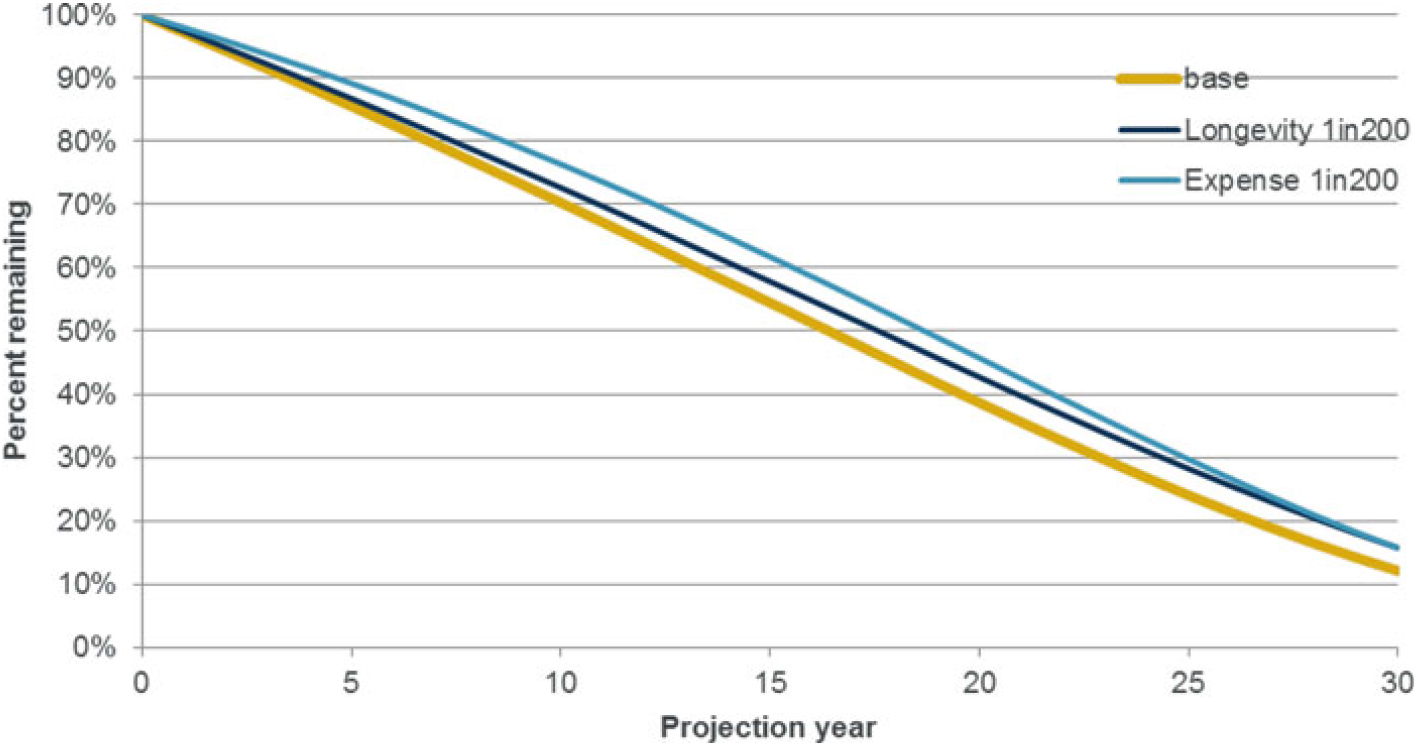
The results show that the run-off rate may be significantly slowed down under a longevity or expense stress. (The graph also highlights the differences that may arise to the shape of the run-off.) The longevity event and expense event have similar effects over the longer terms, whereas the expense stress effects are strongest at the shorter terms. Although the graph shows non-market risks, the effects of market risks such as inflation or interest rates may also be significant.
7.3.3 In addition to the risk drivers, the other key elements of the calculation are the valuation of time zero SCRs and the discount rate used to discount the future projected SCRs. To derive these, the approach described above for the SF SCRs (section 6) has been used (allowing for longevity and expense risk only in the SCR calculations). For the discounting, the discount rates under stress have been calculated to allow for the interest stresses as defined.
7.4 RM fitting SF example – Results
7.4.1 A proxy function has been fitted to changes in the SF RM for the annuity model. The approach used is the same as that set out for the SF SCR in section 6 (using 1,023 calibration runs). The fitting results graph is as follows:
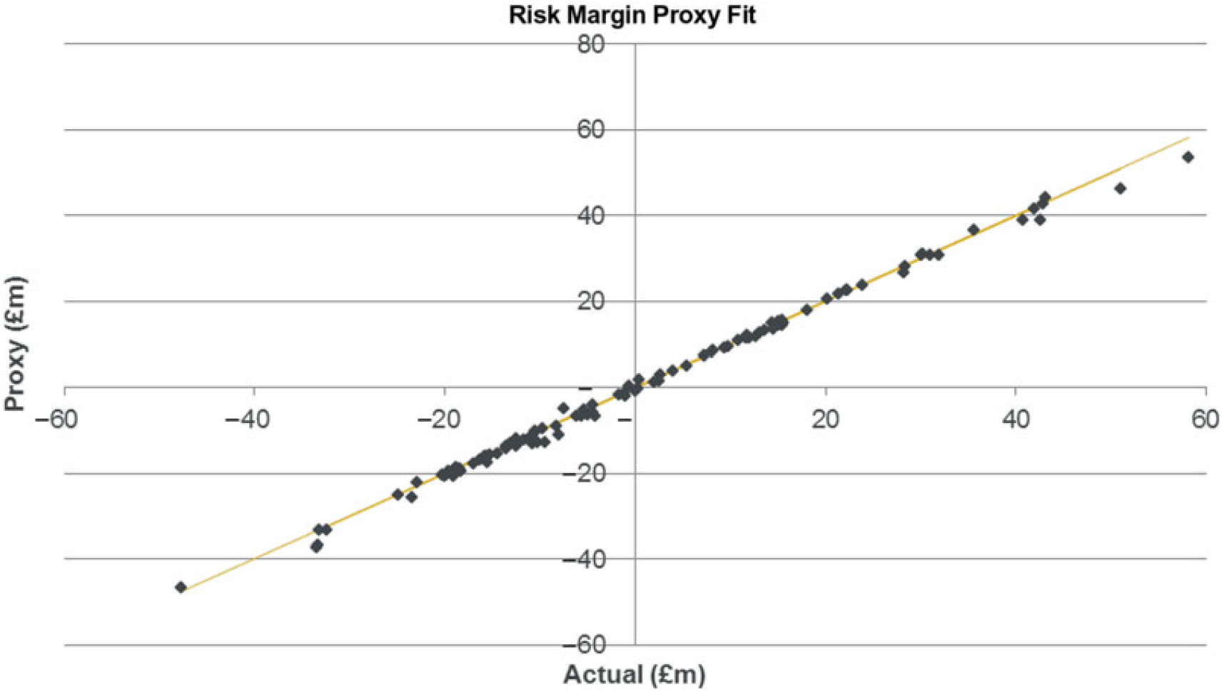
The results have been considered sufficiently accurate, and so the calibration has been accepted.
7.5 RM fitting SF example – Key exposures
7.5.1 The following graphs show the key exposures of the RM:

7.5.2 The results show a significant exposure to falling interest rates as a result of increased projected longevity and expense capital, together with lower discounting. Exposure to expense and inflation increases are also significant due to changes in the projected expense risk capital.
7.5.3 There is an exposure to longevity risk due to increases in the projected expense and longevity capital together with changes in the run-off. The exposure is smaller than for expense or inflation risk due to differences in the run-off pattern. The run-off graph above shows inforce volumes are much higher for expense risk than longevity at the 10-year point, but they converge by the 30-year point.
7.6 TMTP fitting
7.6.1 The TMTPs are the transitional measure designed to allow for changes between the Solvency I and Solvency II regimes amortised over a 16-year period. The amount of TMTP reflects key differences such as the inclusion of the RM under SII and differences in the BEL such as allowances for illiquidity premia. The amount of TMTP steps down using increments of  ${1 \over {16}}$ each year over the transition period. The TMTP amount may be recalculated subject to regulatory requirements and approval. The amount of TMTP is subject to the financial resources requirement (FRR) test designed to ensure firms are not better off than under SI allowing for the TMTP.
7.6.2 If the TMTP amount was not be expected to be recalculated, it would not be necessary to include the TMTP in a stochastic full balance sheet model as it is not risk dependent. The simplest approach to the allowance for any TMTP would therefore be to assume no recalibration.
7.6.3 In practice, the TMTP would be expected to be recalculated under specific circumstances. The PRA has indicated that it expects TMTP to be recalculated every 2 years or following a material change in risk profile.Footnote 23
7.6.4 A material change in risk profile could arise from a large risk movement such as a significant interest rate fall. Firms may have documented practice that sets out what criteria they consider represents a material change in risk profile. However, any recalculation would still be the subject of regulatory approval.
7.6.5 In view of the above, firms may consider that the 1-in-X type of events included in their risk appetite statements would constitute a change in risk profile; therefore, it would be necessary to include an allowance for TMTP changes in their full balance sheet model. Alternatively, firms may consider it inappropriate to speculate that TMTP may be recalculated as this may then give the firm a reliance on recalculation when this may not happen in practice (or may not happen quickly enough). In either case, it is important for firms to consider whether their stochastic full balance sheet model should allow for changing TMTP in order that risk appetite or other risk management modelling can be effectively carried out. Firms may choose to investigate results both including and excluding a TMTP recalculation.
7.6.6 Should an allowance for TMTP recalculation be made in the stochastic full balance sheet model, it is necessary to identify a suitable approach to allow for it. For many firms, the most significant element may be the RM. This may be easily allowed for as the TMTP amount represents the  ${a \over {16}}$
of the RM where a reflects the number of year of transition remaining. However, there are some complexities that need to be taken into account such as that the TMTP applies only on business written before the 1st January 2016.
${a \over {16}}$
of the RM where a reflects the number of year of transition remaining. However, there are some complexities that need to be taken into account such as that the TMTP applies only on business written before the 1st January 2016.
7.6.7 Where other elements of the TMTP are material, the approach used to allow for them would differ depending on the nature of the model. The allowance for the FRR test (where this has an effect) may be complex to allow for.
7.6.8 In the example model, no changes in the value of TMTP are taken into account.
8. Combined results – SF model
8.1 Purpose
8.1.2 In the above sections, proxy functions for the net assets, SCR and RM under the SII SF have been derived. This short section shows how the results combine to give the overall balance sheet exposure.
8.2 Key exposures
8.2.1 The following graphs show the key exposures of the model. For comparison purposes, the graphs show the full balance sheet exposure and also the net asset exposure (just the changes in assets and liabilities) so that the importance of modelling all elements of the balance sheet can be seen.

8.2.2 The results show a significant difference in interest rate exposure for the full balance sheet as compared to the net assets only. The reason for the difference is the significant exposure to falling interest rates in the SCR and RM.
8.2.3 Longevity results show the full balance sheet exposure is very close to the net asset exposure. This is due to the SCR and RM elements being in opposite direction in this particular example.
8.2.4 The inflation and expense exposures are significantly increased in the full balance sheet model compared to the net assets. This is because increases in inflation or expenses give increases to SCR and RM as well as the cost of the annuities.
8.2.5 It should be noted that these exposures are very specific to the example used. Each model or set of parameters could possibly give very different results (e.g. longevity exposure in a full balance sheet model may be more onerous than the net assets results suggest).
9. Discount rates modelling
9.1 Purpose
9.1.1 The purpose of this section is to discuss the effects of changes in key discount rates in a stochastic full balance sheet model in order that their effects may be realistically quantified. The key features discussed are the VA, MA and pension scheme discount rates.
9.2 Volatility adjustment
9.2.1 The volatility adjustment or VA represents a flat addition to the discount rate for applicable long-term liabilities.Footnote 24 The VA was introduced as part of EIOPA’s long-term guarantees (LTG) package alongside other features such as the MA and transitional measures. The VA is designed to prevent pro-cyclicality by removing “artificial volatility” from the Own Funds of insurers.
9.2.2 The VA is calculated using 65% of the spread between the interest rate of the assets in a reference portfolio and the risk-free rate, allowing for a fundamental spread (FS). The FS represents the element of the spread attributable to default and downgrades.
9.2.3 The VA is published monthly by the European Insurance and Occupational Pensions Authority (EIOPA) according to a defined formula. The calculation is carried out separately by duration and rating with the results used to derive a single VA. Allowance is also made for separate country-specific effects where significant.
9.2.4 The VA may be used by firms on specific areas of business subject to regulatory approval. Firm’s RM calculations are required to exclude the VA.
9.2.5 The approach to the allowance for the VA with firm’s SCR calculations varies across Europe. The UK regulator does not currently permit the VA to be allowed to change under SCR stresses. However, the use of a dynamic VA in the UK is under consultation at the time of writing. It should be noted that should a dynamic VA be adopted, there may be restrictions on its use to the extent that firms may consider using a different dynamic VA model within a full balance sheet model.
9.2.6 As described above, in the UK regulatory regime there are therefore three different modelling treatments:
• In the valuation of net assets, the VA is included.
• In the SCR calculation, the VA is included but cannot change under stress.
• In the RM calculation, the VA is excluded.
9.2.7 The use of a static VA in (UK) SCR calculations gives the implication that the SCR calculations do not permit VA changes, but in practice the VA moves in response to spread movements according to its prescribed formula. For this reason, the proxy functions a firm may use for its IM calculations on VA business are not suitable for use in a stochastic full balance sheet model.
9.2.8 To be able to effectively model VA business in a full balance sheet model, it is necessary to use proxy functions calibrated to allow for a dynamic VA. One approach is to recalibrate a dynamic VA proxy function. However, if proxy functions exist without allowance for a dynamic VA (as used in the SCR), an alternative approach can be used that can avoid the need for new runs. This is to estimate the effects that the VA may have by deriving a linear combination of interest rate PCs as an approximation to the VA using the techniques discussed in section 6.3.Footnote 25 The graph below demonstrates how a 1% stress to the interest rate curve may be approximated using a combination of three PCs.
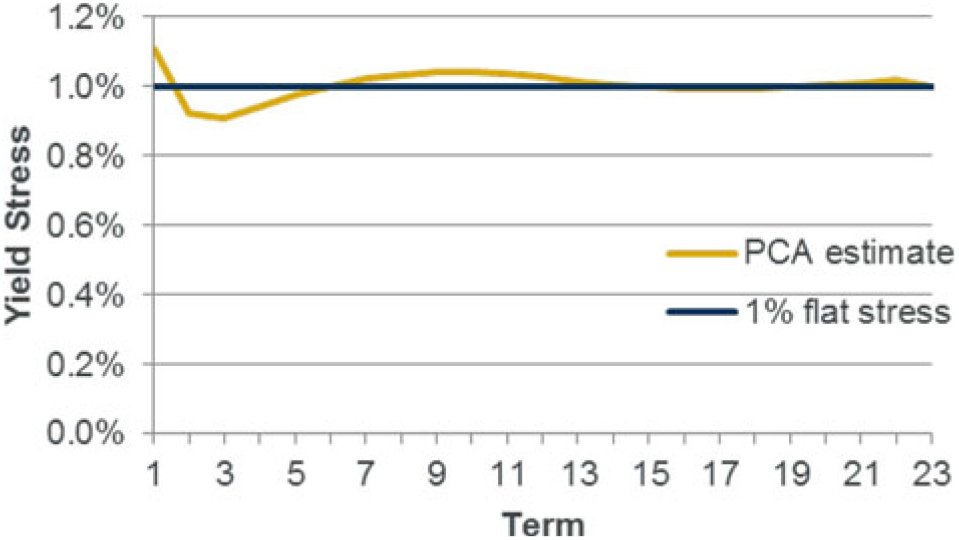
9.2.9 Where firms use copula simulation models for their SCR calculations, an SCR proxy function may be calibrated using the roll forward–based approach discussed in section 6. However, it is important here that the roll forward process takes into account a dynamic VA, but the resulting SCR calculations use a static VA. This may be done, for example, by rolling forward the (dynamic VA) proxy functions as normal before setting any credit risk elements of the proxy function to zero for the VA liability element of the proxy function.Footnote 26
9.2.10 For a firm’s RM, this is calibrated without VA. Firms in the industry typically use a risk driver approach for the RM calculation in which an initial SCR in respect of non-hedgeable risks is projected to future years. Where such an approach is used, the initial SCR needs to be calculated without VA. Proxy functions that exclude VA can be derived from those that include it through techniques such as those shown in section 9.2.8.
9.2.11 Firms that use variance covariance–based approaches to SCR such as those used in the SF would need to use an approach equivalent to those described for simulation approaches. Therefore, a dynamic VA would be used in the roll forward process used to derive the SCR, but the SCR itself would assume a static VA. The RM would, of course, not allow for VA.
9.3 Dynamic VA model
9.3.1 To be able to use above techniques we require a dynamic VA model. This is a model that is used to estimate how the VA moves in response to the spread stresses.Footnote 27 At its simplest the model could take the form of:
Change in VA = 65% Change in spreads.
A more detailed form of model would take into account the effects at different ratings and durations and reproduce the full EIOPA–specified calculations to derive the VA.
9.3.2 The main elements of the VA calculation can be modelled by allowing for the credit risk changes in the risk model in the VA calculation. One aspect that requires further attention is the FS underlying the calculation and used to represent default and downgrades. The concept of the FS is common to the VA and also the MA.
9.3.3 In the context of the MA, the allowance for changes in FSs has been discussed in detail by the PRA. In SS8/18, the PRA set out its expectations that in the IM SCR calculation firms should not use a purely “mechanistic” approach to determine the FS following a stress. In view of the PRA expectations, IM firms that use an MA have since developed models of the FS under stress. These models normally use an approach under which EIOPA’s specified calculation of the FS remains the same, but the parameters used within are adjusted to represent stressed conditions.
9.3.4 Firms that already use a model of the FS in their MA calculations may be able to also use this for a stochastic full balance sheet model. However, it is important that the model is able to realistically allow for changes in the FS for small or moderate changes as well as the extreme stresses that are important under a firm’s SCR calculation. Such small or moderate credit events give rise to low materiality changes in the FS as the probability of default, cost of downgrade and long-term average spread elements of the calculation take into account a long time frame.
9.3.5 It is important in a stochastic full balance sheet model to consider whether the framework set out by the PRA for use in IM MA calculations aligns with their own realistic views.
9.3.6 The graphs below give some examples of how the FS may change in response to credit stresses under different models. These graphs are a simplified representation of a full FS model (e.g. a full FS model would normally be carried out by duration and rating).
9.3.7 Flat FS model
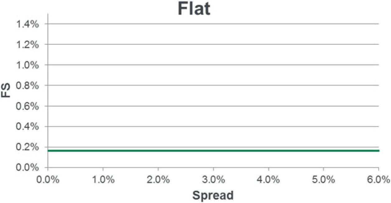
A flat FS model such as this assumes no changes in the FS in response to spread stresses. Such a model would be unlikely to be permitted by the regulator for use in a firm’s MA under stress calculations as it does not take into account possible changes of the FS. However, this does not necessarily mean the model is not appropriate for use in a full balance sheet model.
9.3.8 Linear FS model

Under this model, the FS increase linearly with spreads. To calibrate such a model, an extreme scenario such as that at the 1-in-200 could be considered in detail, with the FS behaviour away from this point linearly modelled. The model has the advantage of simplicity. However, the behaviour at moderate stress movements is unlikely to be realistic. In practice, the FS used in the VA calculation would remain materially unchanged under moderate stresses. A non-mechanistic change would be expected to be made only in response to more material market events in accordance with EIOPA’s internal governance procedures. A moderate change would be unlikely to give a reason for such a change.
9.3.9 Split FS model

A model such as this gives the desired effect of no changes for moderate stress while allowing for increases under large spread events. Allowing for a specific change in the function at a particular spread level may be a disadvantage as in reality there is no clear point at which a step change would occur.
9.3.10 Power function model
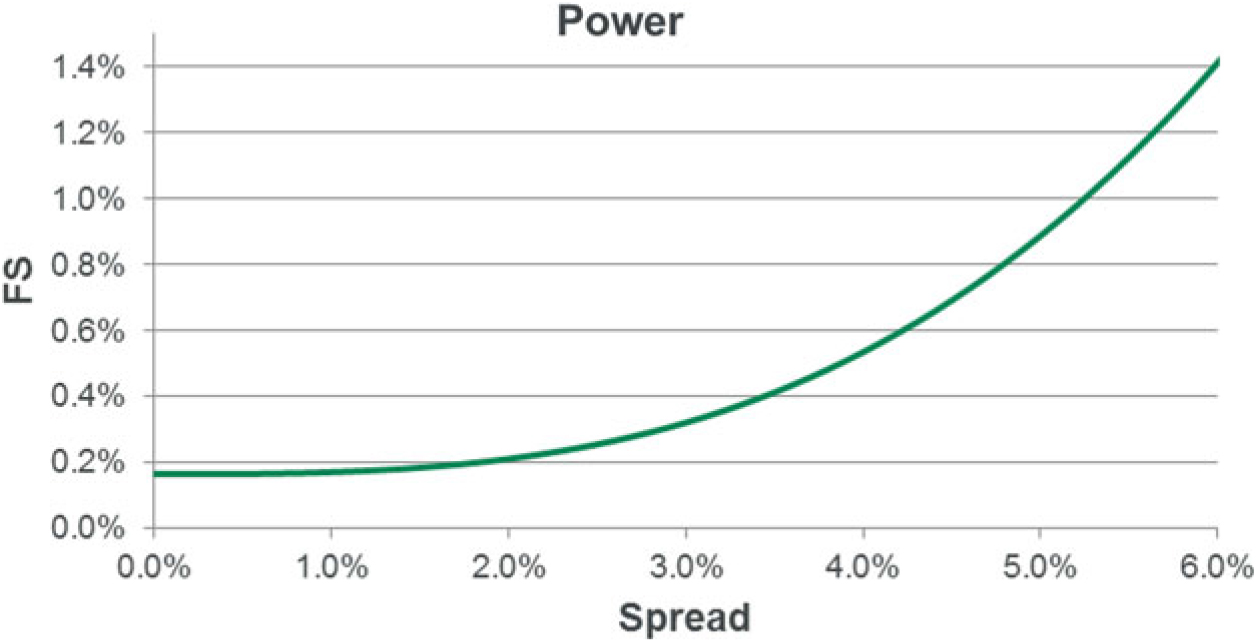
A model such as this gives no material change for moderate stresses and an increase in FS at the more extreme levels. It also has the advantage of having a smooth curve rather than a fixed change point. The model has the disadvantages that it may be difficult to parameterise and that at very extreme spread stresses (such as beyond the 1-in-200 level), the FS may increase to the extent that the VA is removed altogether. Where the FS are used for an MA calculation, this may be considered to be a point at which conditions are so extreme; it is no longer possible to meet the MA qualifying criteria, and so the MA can no longer be used.
9.3.11 The above FS models show a number of the considerations in the design of the FS model. While it is clear that the FS would remain materially unchanged under small stresses, the most challenging consideration is perhaps how changes in the FS should be modelled under large credit stress events. This is a difficult aspect to effectively allow for as it requires assumptions to be made for how and under what circumstances EIOPA may change the FS.
9.3.12 One view on changes in FS is that, the whole purpose of the VA is to protect against “artificial volatility”. If a severe credit event were to occur, then any increase to the FS at that time could have a highly pro-cyclical effect and therefore result in the opposite to what the VA is designed to do. This would not be consistent with one of the original objectives of SII to give financial stability.
9.3.13 An alternative view is that the full balance sheet model should allow for possible adverse changes to the regulations in extreme events, since to do otherwise places reliance on EIOPA prioritising stabilising behaviour over other objectives in a time of crisis. While EIOPA may indeed take into account these considerations under extreme conditions, it may not be considered prudent for a firm to place reliance on these.
9.3.14 A key point here is that effective communication of the assumptions of the model and limitations are of great importance. If a stochastic full balance sheet model were to be based on the assumption of no change in the FS, it should be made clear that this is a key assumption and the risks associated with the assumption should be discussed.
9.4 Matching adjustment
9.4.1 The matching adjustment or MA has a similar effect to the VA. It represents a flat increase to the discount rates to be used on long-term business matched with a specific set of assets (the MA portfolio or MAP). The MA originated to allow UK annuity providers to allow for the illiquidity premium in respect of assets held to maturity. Whereas the VA is calculated by EIOPA to reflect representative assets for different countries, the MA is instead calculated using the actual assets in a firm’s MAP.
9.4.2 In simple terms, the MA is calculated using the spread of the assets in the MAP with a reduction to allow for the FS as used under the VA calculation. The MA is subject to regulatory approval for which a set of qualifying conditions need to be met. The MA and VA cannot be applied on the same business.
9.4.3 Unlike the VA, the MA is permitted to change under SCR stress. The manner in which it changes under stress is prescribed under the SF but calculated according to firm’s own approach under IM. The PRA has published a framework to set out how the MA under stress could be calculated. The RM does not take into account the MA.
9.4.4 In summary, under a stochastic full balance sheet model it is necessary to be able to model changes in the MA as affecting the liabilities and the SCR. The full balance sheet model may or may not use the same approach to allowance under stress as is used under a firm’s SCR (IM or SF). If a different approach is used, it is necessary that the SCR proxy function is calibrated using the SF or approved IM approach.
9.4.5 To allow for the MA in a stochastic full balance sheet model in practice, a model of the FS is again required. For consistency, the model should be aligned with the FS model used for any VA calculations (if a firm uses both the VA and MA). Using the FS model, the MA calculations for any given stress can be repeated to give a stressed MA valuation.
9.4.6 One difficulty that may arise is that the framework set out by the PRA may not be practically carried out for a high volume of stresses as it includes the analysis of the results of stress scenarios in order to see if the MA qualifying conditions still hold and whether there would be a cost associated with re-establishing an MA compliant portfolio. One possible solution to this problem is to calibrate an MA proxy function using a small number of runs and to use this to approximate the MA under the full calibration set for the MA liabilities.
9.5 Pension schemes’ discount rates
9.5.1 Defined benefit pension schemes are normally modelled using the IAS19 basis under SII.Footnote 28 The discount rates under the IAS19 basis reflect the yield on high-quality corporate bonds (typically taken to mean AA rated) for which there is a deep and liquid market.
9.5.2 Under credit stress events, the PRA has set out its expectations that it may consider it appropriate that a proportion (rather than the full amount) of the credit stress is reflected in the discount rates under firms IM SCR calculations. This is to take into account that:
• Bonds may be affected by defaults and downgrades.
• There may not be a deep market for high-quality corporates following a stress event.
• Any significant divergence between the scheme funding and IAS19 bases could result in the need for additional contributions.
9.5.3 For IM firms, it would therefore be expected that the IM already includes an allowance for changes to the IAS19 discount rates under stress. This model may also be used in a stochastic full balance sheet model. However, it is necessary to take into account that the model should be accurate for small or moderate stresses as well as for the extreme stresses that may be key to the SCR. For small to moderate stresses it is likely that the IAS19 discount rates reflect the full change in spread.
9.5.4 For practical reasons, it is helpful if a firm’s realistic modelling of the IAS19 discount rate is aligned between the IM and stochastic full balance sheet model. However, a bespoke calculation for the full balance sheet model may be considered if the IM approach would not be considered to be fully realistic.
9.5.5 For SF firms, no changes in the IAS19 discount rates are taken into account under SCR credit stress events. It is therefore necessary to include a model of how the IAS19 discount rates vary under stress for use in the full balance sheet model. Of course, within the SCR proxy calibrations, no allowance for changes in the discount rates under credit stress should be permitted.
9.5.6 The following graph shows the results of a possible example model of the IAS19 discount rate changes.
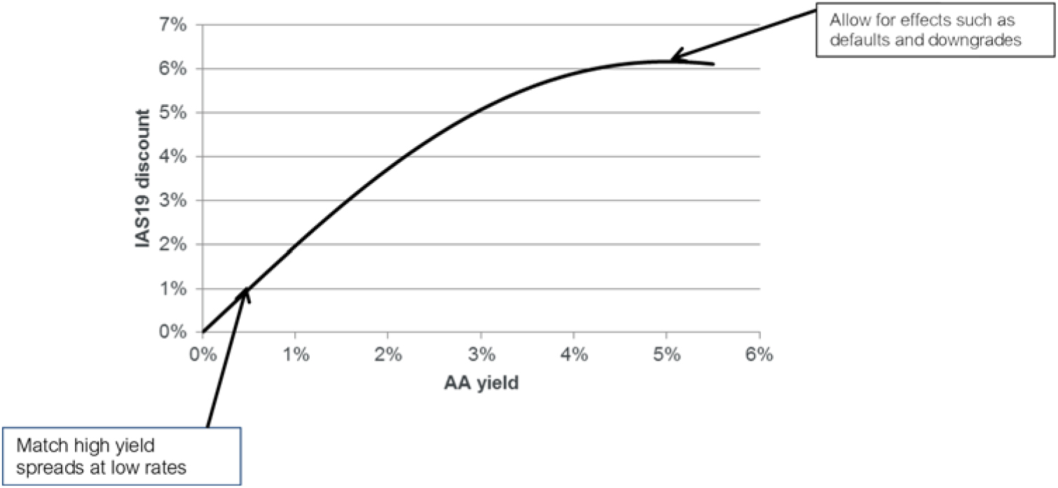
9.6 VA in annuity example model
9.6.1 In order to demonstrate how the above techniques may be used, an allowance for a VA has been introduced to the annuity model described above. The VA model is designed as follows:
 $${\rm VA} = 0.65^*w^*\,( {S-{\rm F}{{\rm S}_S}})$$
Where w is a constant of 0.331Footnote 29
S is the spread
FSS is the fundamental spread for spread S
FSs is specified as 0.163% + 0.5max(S – 3.5%,0) (the split FS model)
The FS model and VA model can be seen in the following graphs:
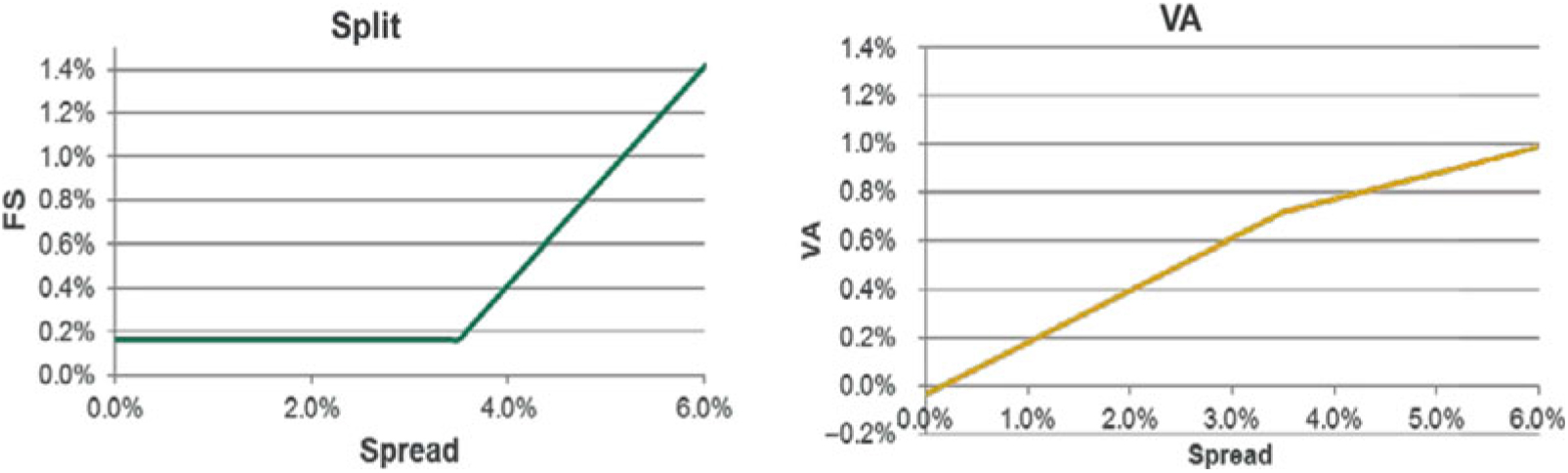
9.6.2 Note that this is a model in which the VA and FS are specified as a function of spreads, rather than changes in spreads. The annuity example used in this paper uses a credit risk distribution based on changes in spreads. Therefore to complete the model, it is necessary to also specify the current spread. A current spread value of 1% has been assumed.
9.6.3 Using the VA model, the annuity proxy models for the net assets and SF SCR have been refitted (the RM proxy is unchanged as it is not affected by VA).
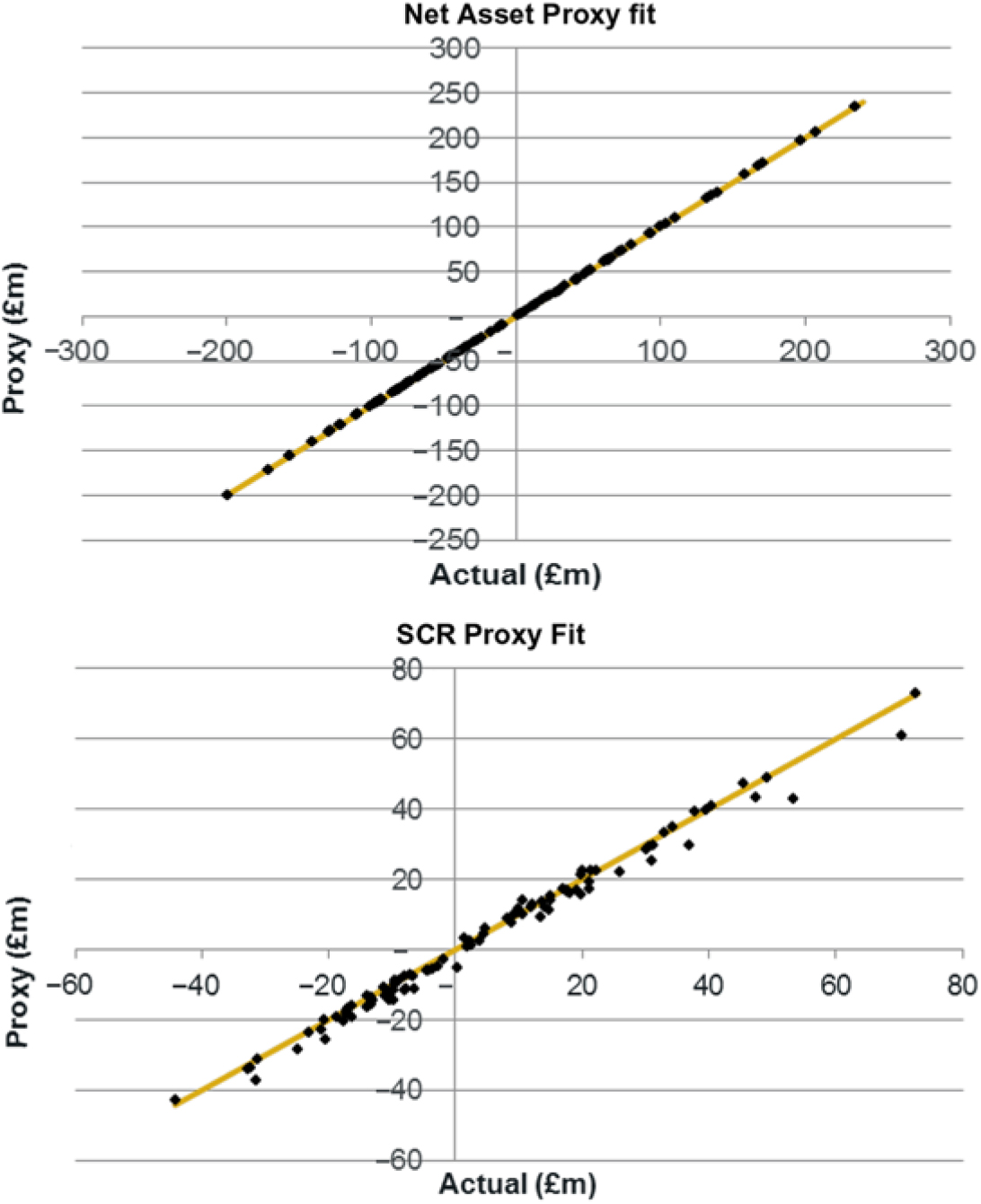
The proxy calibrations show the fit is acceptable. The SCR fit is not as close as previously as the introduction of the VA gives credit exposure. This makes the fit more challenging both as it increases the dimension of the proxy function, and because the credit exposure itself has an unusual form as results from the split FS model used.
9.6.4 The following graph shows the credit risk exposure in the new proxy model (the exposure to other risks in the proxy functions is materially unchanged from before).
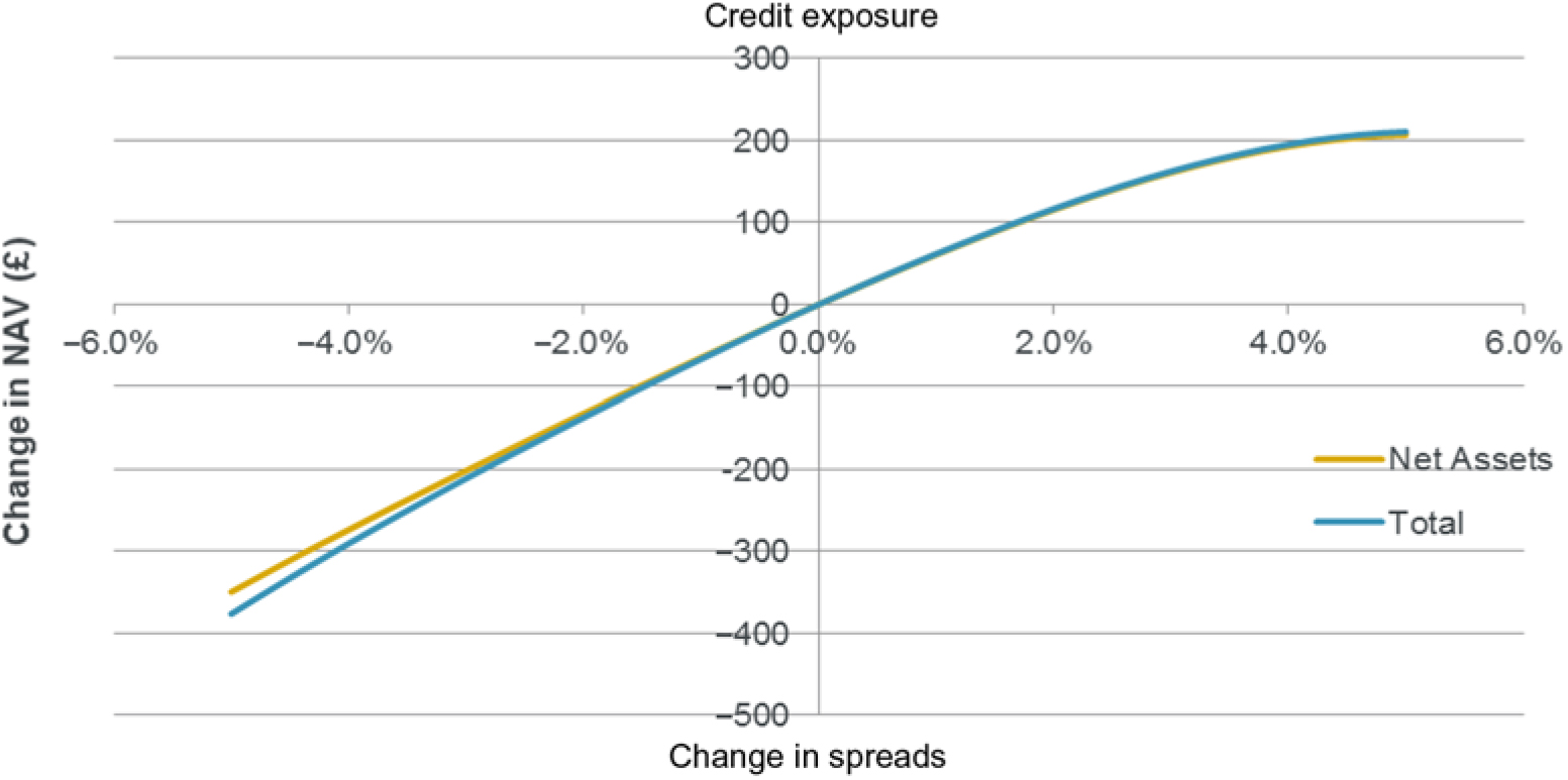
9.6.5 The results show a very significant exposure to falling spreads through the reduction in VA this gives. In practice, most VA business would be backed with a proportion of corporate bond assets and so such an unmatched exposure on the liabilities would be unlikely. However, it is likely that many firms have assets matching VA business that are very unlike the representative portfolios of bonds used in the EIOPA calculations and so significant credit exposures are possible.
9.6.6 The results show only small differences between the total losses (the full balance sheet model) and the net assets. However, in this case the net assets use the dynamic VA model above. There would, of course, be large differences compared to the proxy functions used in a firm’s IM SCR.
9.6.7 The exposure graph shows the gradient of the curve reducing at high spreads. This is a result of the dynamic VA model used.
10. Example model results
10.1 Purpose
10.1.1 The purpose of this section is to show how the example proxy model introduced above can be used to find key measures such as the 1-in-X events used in risk appetite. The version of the example model used here includes the VA with SCR according to the SF.
10.1.2 The assumptions discussed in section 4 above include that the example firm has a starting surplus of £250m. Its risk appetite framework includes that it is able to withstand a 1-in-30 shock over a 1-year time horizon. A fall below a 1-in-10 level triggers urgent corrective action.
10.2 Risk appetite 1-in-X results
10.2.1 Using these assumptions, the probability distribution of changes in the firm’s surplus based on 100,000 simulations is shown below with the risk appetite boundaries.
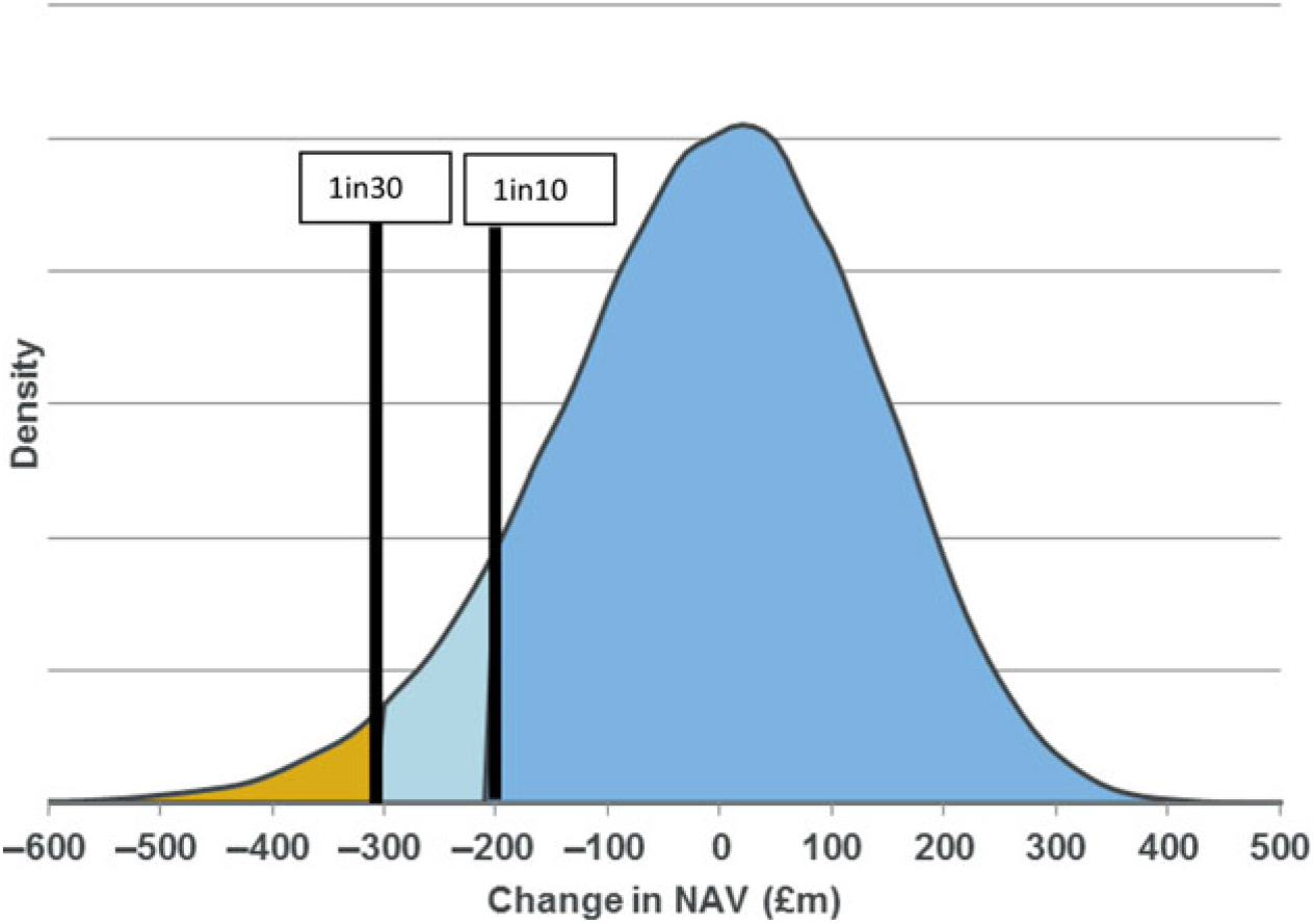
10.2.2 The following graph shows the risk appetite in an alternative form:
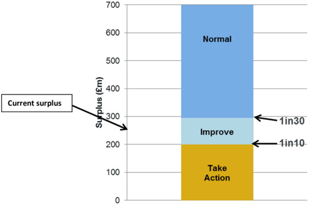
The results show the current surplus leaves the firm in the “improve” zone. The firm may therefore start to consider corrective steps to improve the surplus, but urgent action is not yet required.
10.3 Ruin probability results
10.3.1 In addition to looking at risk appetite 1-in-X results, it is important for risk management purposes to understand the ruin probability over the 1-year time frame.
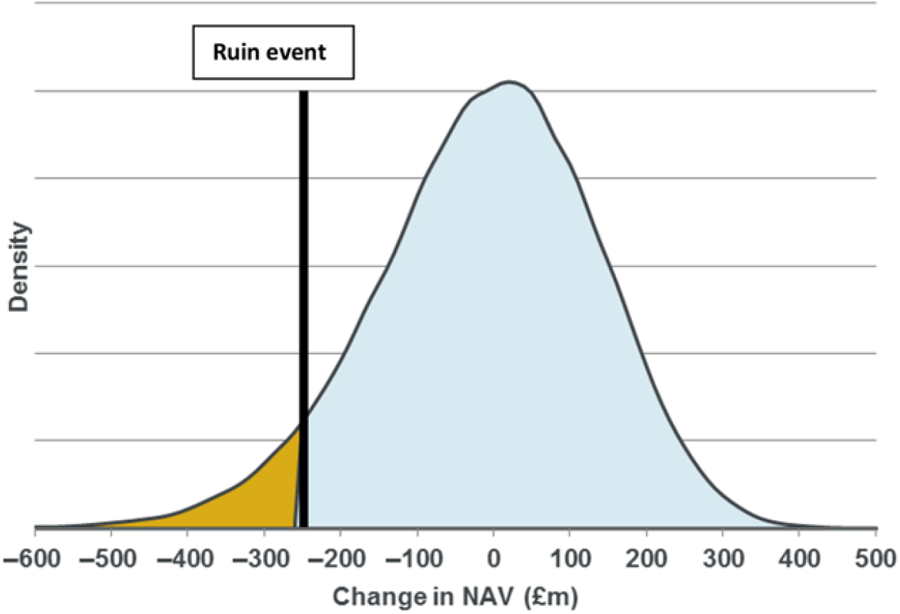
The ruin probability in this case is 5.9%. By finding this ruin probability, the firm is then able to identify what steps (e.g. reinsurance) it may be able to take to manage the ruin probability within an acceptable level.
10.4 Euler allocation
10.4.1 Having identified the ruin probability, a firm may wish to analyse which business elements (e.g. products and sub-companies) may be the cause of the ruin event. This may be carried out using standard Euler allocation techniques. For a VaR measure (Tasche, Reference Tasche2004):
 $${A_p} = - E({X_A}|{X_{\rm total}} = - {\rm Va}{{\rm R}_p})$$
Here A is the Euler allocation for business unit A at percentile p. X A is the change in value for business unit A, X total is the change in value over all business units. Of course other allocation approaches may also be considered, but Euler allocation is the standard technique.
10.4.2 This approach may be used within a stochastic full balance sheet model to break down risk appetite 1-in-X or ruin losses by balance sheet elements such as the value of different assets, liabilities, SCR and RM. If necessary, changes in the SCR and RM could be further split by the asset and liability changes within.
10.4.3 In practice, to apply the Euler allocation approach within a simulation model, it is necessary to construct a kernel of simulations. This is a set of simulations in the region of the loss amount to be assessed (e.g. the 1-in-30 risk appetite loss). A weighting (known as a kernel smoothing filter) is normally applied to the kernel in order that greater reliance is placed on the simulations closest to the required value.
10.4.4 In addition to investigating losses by business unit, it is useful for firms to be able to understand the contribution of each risk to the overall loss. A standard approach to this is to again use the Euler allocation method to determine the expected source of the losses. When using proxy functions, an important question here is how to allow for cross terms (terms of more than one risk) in the proxy function. The approach used depends on the purpose of the analysis. It may be appropriate to separately show these or use an apportionment approach to apply them to the constituent risks.
10.4.5 The following graph shows an Euler allocation by risk of the £250m loss associated with the ruin event in the annuity example:
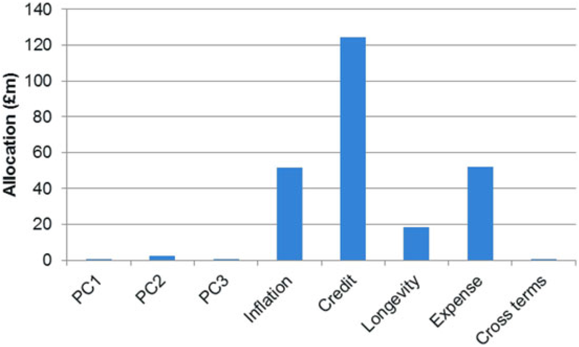
10.4.6 The graph shows that the expected losses come mostly from credit risk (exposure to spreads falling due to the VA), with important contributions from longevity, inflation and expense risks. The interest rate expected losses are low. A key reason for this is that credit is the dominant risk in the model, with interest rate PC1 negatively correlated with credit. This means that even though interest rate falls give a significant cost, they do not have a high contribution. The cross terms in the graph are also low. However, there are many offsetting amounts within the total.
10.4.7 The assumed investment strategy in the example is that the assets are risk free. As a result of this, the exposure to credit risk results from changes in the VA giving rise to liability changes without an equivalent asset change. In practice, the exposure to credit risk would be highly dependent on the assumed investment mix. For example, if an annuity portfolio was backed by assets similar in nature to the representative portfolios underlying the VA, the exposure to credit risk would be far smaller.
10.4.8 The above points demonstrate a limitation with the use of Euler allocations to analyse the ruin events. The limitation results from the use of expectations in the Euler calculations. Simply looking at the above graph, the conclusion may be that interest rate risk is unimportant and cross terms immaterial, so combined risk events are not a key concern. However, in practice there may be a significant risk associated with interest rates falling (as the risk exposures above show in section 8). Cross terms may also be important.
10.4.9 To illustrate the limitations of the Euler allocation, the following table shows the losses under the six scenarios closest to the £250m ruin event:

10.4.10 The table shows the significant amount of variation in these scenarios that cannot be seen from the Euler allocations. Three of the scenarios are credit dominated, and there are others that are more expense- or inflation-led scenarios. Note how the cross terms above may actually be very significant.
11. Ruin events
11.1 Purpose
The purpose of this section is to discuss the limitation of using Euler allocation and show how analysis of actual ruin events may give greater insight.
11.1.1 The key point with Euler allocation is that it provides an allocation of the total amount of capital a firm may hold in respect of different business units or risks. An Euler allocation does not give a clear insight into the actual risk events that may cause a particular loss (such as the ruin event). It also may obscure the extent of variation in the types of events that may cause the loss.
11.2 Simple two-risk example
11.2.1 As an example, consider a model with two risks A and B. The risk model is multivariate standard normal with the correlation between A and B equal to −99.9%. The loss function used sets the change in NAV = 2 – (eA + eB) £m.
In this example B is expected to be very close to –A at all times due to the correlation used. This means the loss function graph is close to the following:

Therefore, this example gives small losses for A (and B) close to zero, but the losses increase further for large or small A (and therefore small or large B). Where there are significant losses, these almost all come from either risk A or risk B.
11.2.2 The capital for a 99.5th percentile VaR metric in this model is around £14.8m (obtained by generating simulations in the manner shown above). Due to the symmetry of the model, the Euler allocations of the capital are £7.4m to each of risks A and B.
11.2.3 It should be noted that the results of the Euler allocation do not give a helpful insight into the kind of events that could cause the VaR loss. The event at which losses of 7.4m occur on both risks A and B corresponds to A and B both being equal to around 2.1. However, due to the correlation of −99.9% being used, this event is near-impossible.
11.3 Most likely ruin events
11.3.1 The MLRE is defined to be the event with the highest probability density within the set of ruin events (the ruin region).Footnote 30 The set of ruin events is the set of events under which the loss is greater than the starting surplus.
11.3.2 Using a model with a single risk, the MLRE can be seen in the graph below:
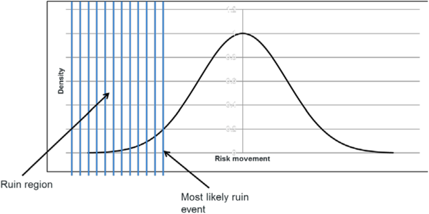
11.3.3 For a model with two risks, a 3d or contour-style plot can be used as below:
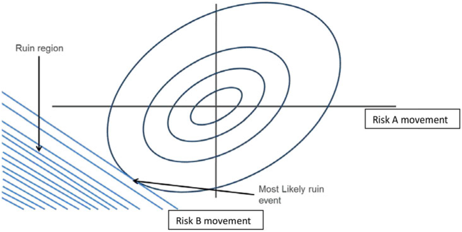
11.3.4 The graph contains two different measures overlaid, the probability density function and the ruin region.
11.3.5 The probability density function is represented by the contours on the graph used to show points of equal probability density. The highest probabilities are at the centre with decreasing values for increasing (positive or negative) risk movements. The shape in this example is characteristic of a positive correlation between risks.
11.3.6 The ruin region on the graph is shown by the blue shaded area. This area represents all combinations of the two risks for which the losses exceed the initial surplus. In this example, the edge of the ruin region is a straight line. This indicates that the loss function used in the example is a linear function of the two risks.
11.3.7 The MLRE can be seen as the point with the highest probability density in the ruin region.
11.4 MLRE applied to the two-risk example
11.4.1 Using the two-risk example above, if for illustration the starting surplus was £14.8m, the MLRE may be calculated as the point which maximises the probability density f(A, B) over the ruin region.
In this case the probability density f(A, B) is the density of the multivariate standard normal with −99.9% correlation. The density function has a well-documented closed form.
The ruin region here is specified as the region of A,B such that 2 – (eA + eB) < −14.8m.
This represents an optimisation problem that may be solved using standard numerical techniques. The result in this case is that due to the symmetry of the example, there are two equal MLRE points. In any actual model, there will almost certainly be a single MLRE.

The MLRE points are at A, B = (−2.8, 2.8) and (2.8, −2.8).
11.4.2 A plot of the ruin region is as follows:

The line of A = −B on the graph is shown as the correlation of −99.9% means that risk movements will almost certainly be very close to this line.
The graph shows the two MLRE points are where the A = −B line intersects the ruin region.
By identifying the MLRE points, it has been possible to focus on the actual events likely to be the cause of ruin. This is in contrast to the Euler allocation which represents an allocation of the total capital.
11.5 MLRE applied to the annuity example
11.5.1 Using the annuity example model, we may solve for the MLRE in the same manner as has been used for the two-risk example above. This gives the MLRE as the following:
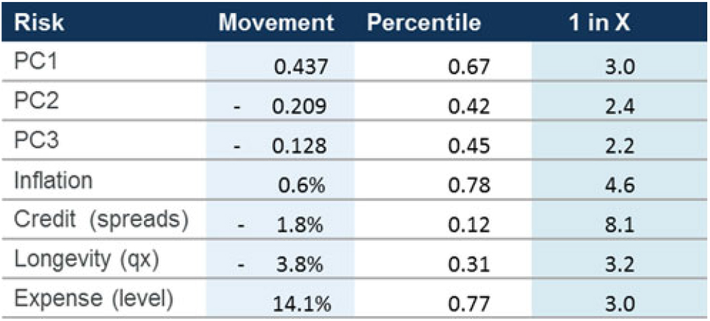
The results show the event is mainly a credit spreads falling event, with inflation, longevity and expense also contributing. The interest rate movements may be better seen through converting the PC movements onto an actual yield curve stress as follows:

11.5.2 An alternative way of looking into the results is to graph the risk movements in relation to a 1-in-X level (e.g. the 1-in-10).

11.5.3 The results may also be viewed in terms of the loss by risk under the MLRE event:
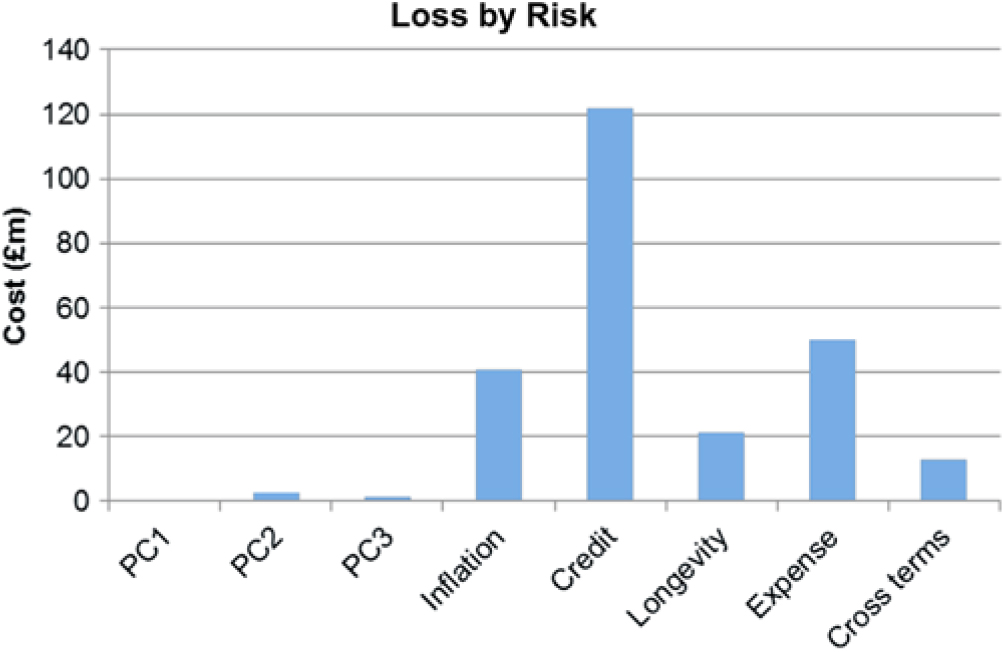
11.5.4 The results in this case show very little exposure to interest rates. For this reason, in the communication of the results, it may be better to exclude these due to materiality and describe the MLRE event instead as a combination of credit spreads narrowing, together with increased longevity, inflation and expenses.
11.5.5 Having derived the MLRE, it is also possible to derive variations of this. For example, the MLRE excluding credit risk or the MLRE using only market risk could be used. It should be noted that, in this case, the MLRE losses are not dissimilar from the Euler allocations. This results largely from the simplicity of the example model and in particular the use of the multivariate normal risk model. An example of an actual firm’s business would not necessarily show the same results.
11.6 Kernel density estimation (KDE)
11.6.1 In the above annuity example, the risk model used was a multivariate normal. Where a well-known parametric distribution such as this with a closed form density is used, then solving for the MLRE can be achieved by maximising the density function over the ruin region. Of course, in practice, firms do not typically use such simple distributions. The distributions used by firms instead normally use a copula to combine a number of different marginal distributions and therefore form the joint distribution of risks. The difficulty this then gives is that the probability density of the distribution does not have a closed form.
11.6.2 Where the probability density function of the joint risk distribution does not have a closed form, then an approach that may be used is to use risk simulation results from the model to derive an estimate for the probability density function. An established technique that may be used for this is KDE (Epanechnikov, Reference Epanechnikov1969)).
11.6.3 KDE is a non-parametric technique that relies on the use of a smoothing function applied to simulation results. The sum of the smoothed results can be used to estimate the density of the overall distribution. The following diagram demonstrates how a normal distributionFootnote 31 smoothing function can be applied to simulation results to generate an estimate of the overall density function. Unlike a histogram approach, KDE normally results in a smooth density function estimate.
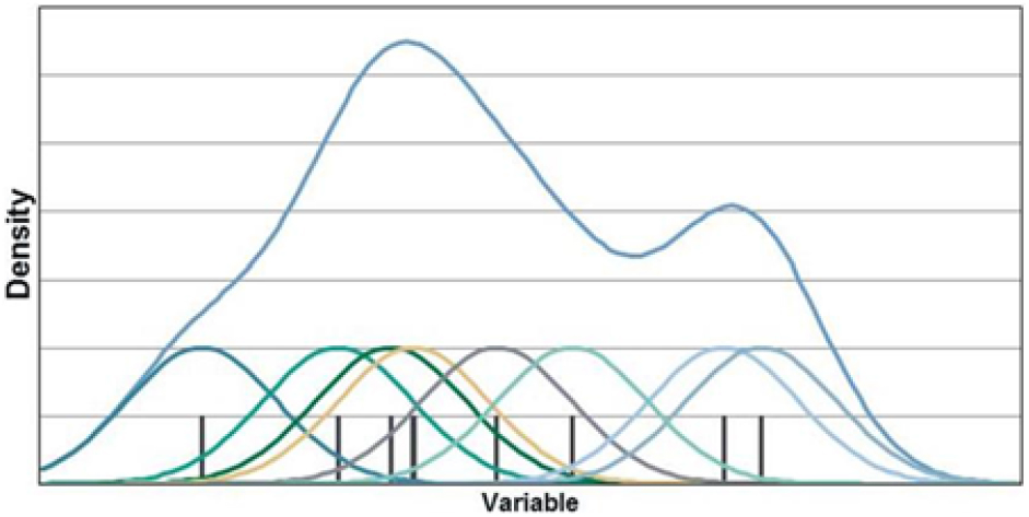
11.6.4 It should be noted that the above graph shows an example in a single dimension. For application in MLRE analysis, KDE in multiple dimensions is required.
11.7 KDE applied to the annuity example
11.7.1 Using KDE as described above, the MLRE losses for the annuity example are shown in the graph below. For comparison, the results of the “direct” approach in which the density function for the multivariate normal distribution is instead used are shown.

11.7.2 The results show a close match between the two events. This is, of course, to be expected as in this case two different techniques have been used on the same model. The purpose of the graph is to demonstrate that the KDE technique may be used effectively and so there is no reliance on being able to directly use the density function.
11.8 Ruin event analysis
11.8.1 As an example of how ruin events can be used in practice, within the annuity example, we may define the key ruin cause using the following approach for any given ruin simulation (i.e. where the loss is around £250m).
1. Identify the largest individual risk loss, if this is greater than 50% of the total loss (i.e. greater than £125m); the key ruin cause is this risk.
2. Consider all possible risk pairs; find the largest loss under each of these pairs allowing for cross terms. If the loss is greater than 50% of the total loss, the key ruin cause is this risk pair.
3. If no single or paired risk event is the cause, specify the cause to be multiple risks.
11.8.2 Using this approach, we may derive the following analysis of the key ruin causes:

11.8.3 As has been explained in section 10.4.7, the dominance of credit risk in the model is largely a result of the assumed investment strategy.
11.8.4 Given the top types of ruin cause have now been determined, we may use the MLRE techniques to identify a precise ruin event that represents each of the five types. For example, we may solve first for the credit event most likely to give ruin, then next the credit and inflation event most likely to give ruin, then the remaining three events.
11.8.5 Having derived the set of such ruin events, these may then be used as the focus of “wargaming” sessions in which business experts consider the appropriate steps that can be taken to mitigate the effects of the risk event or how best to respond to it.
11.8.6 The following table shows the actual most likely ruin events for each of the five identified risk types:

12. Roll forwards and projections
12.1 Purpose
12.1.1 The purpose of this section is to discuss the roll forwards and projections of the model. The two items are discussed in the same section as they are equivalent other than for the difference that a roll forwards process uses actual experience (e.g. economics and run-off), whereas a projection process uses assumptions for future experience. This section discusses the roll forward of proxy functions. It may also be necessary to allow for changes in the risk model within a roll forward process.
12.2 Roll forwards
12.2.1 A roll forwards process is a key part of any proxy model not just a stochastic full balance sheet model. The roll forward process is used to update the proxy functions in the model from the calibration date in which they were first constructed to a “current” date. Note that there may not be a single calibration date for all proxy functions. Instead, different parts of the model may be calibrated on different dates.
12.2.2 There are two key purposes of rolling forward the loss functions. The first is so that the model may always remain current. The second key purpose is so that the roll forward process provides a control cycle on the proxy fitting in the same way as an analysis of change (AoC) provides a key control on valuation results.
12.2.3 It is essential that the process is highly automated and free from any subjective judgements in order that it can be rapidly used to derive the proxy functions for any given date.
12.2.4 A roll forward process needs to take into account all the key items that may materially affect the proxy functions. Examples of these items are as follows:
• Expected run-off of business
• New business
• Economic variances
• Demographic variances
• Basis changes
• Risk model changes
• Model changes
12.2.5 The order of the analysis used for roll forwards can be expected to have a material perceived effect on the results. For example, a change in longevity assumptions may have a greater impact after a model change.
12.2.6 The methods used in the roll forward process are discussed in section 5 above. Changes such as economic variances and basis changes are the equivalent of risk movements. The techniques shown in section 5 can therefore be used to rebase the loss functions. For other elements, different techniques may be applied depending on the nature of the business.
12.2.7 For model changes an approximate adjustment to the loss function is a simple approach that may be used. Where a change is more significant, it may be necessary to recalibrate the proxy function subject to the change. Good governance of a proxy model would require the specification of triggers for which an out-of-cycle proxy model recalibration would be necessary.
12.2.8 The following diagram illustrates the use of the roll forward process as a control cycle.
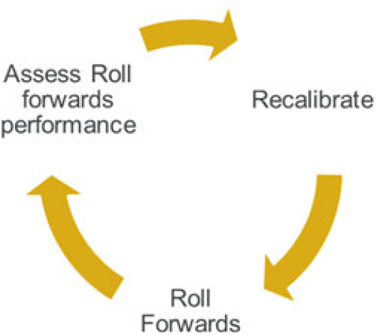
12.2.9 In this process, the loss functions are first calibrated, then roll forwards up to the next calibration point, at which point a new proxy function is calibrated and compared to the rolled forward one. In a perfect process, the newly calibrated proxy function would be the same as the rolled forward one. Of course, in practice there are differences. The extent of these differences is a measure of the performance of the proxy fitting and roll forward processes.
12.2.10 The following graphs show how the change in a proxy function may be assessed by looking at, for example, individual risk graphs and 1-in-20 or other costs.
Base

Allow for run-off
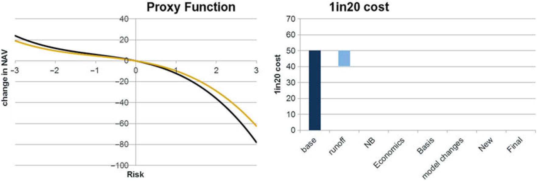
Here the proxy function is scaled down to reflect business run-off through the period.
Allow for new business
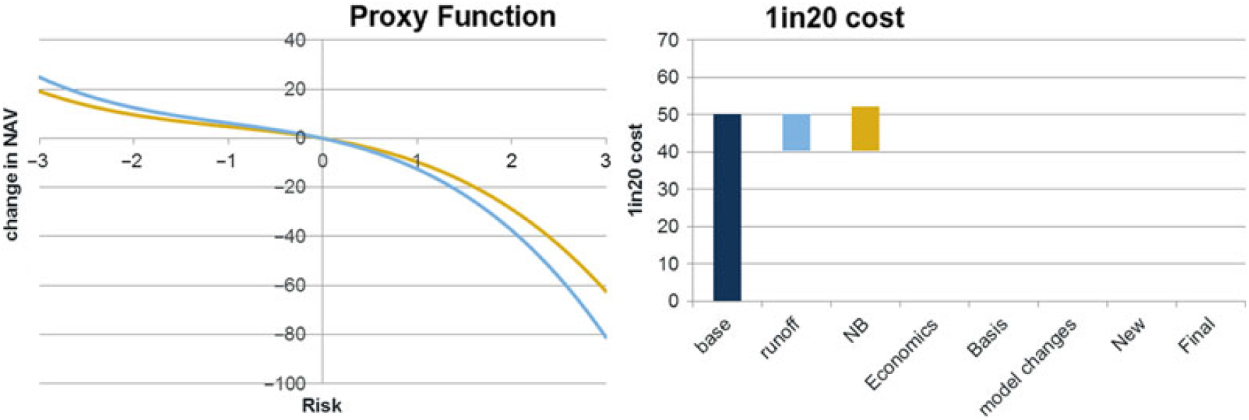
The proxy function is adjusted to reflect the effects of business coming onto the books.
Allow for Economics
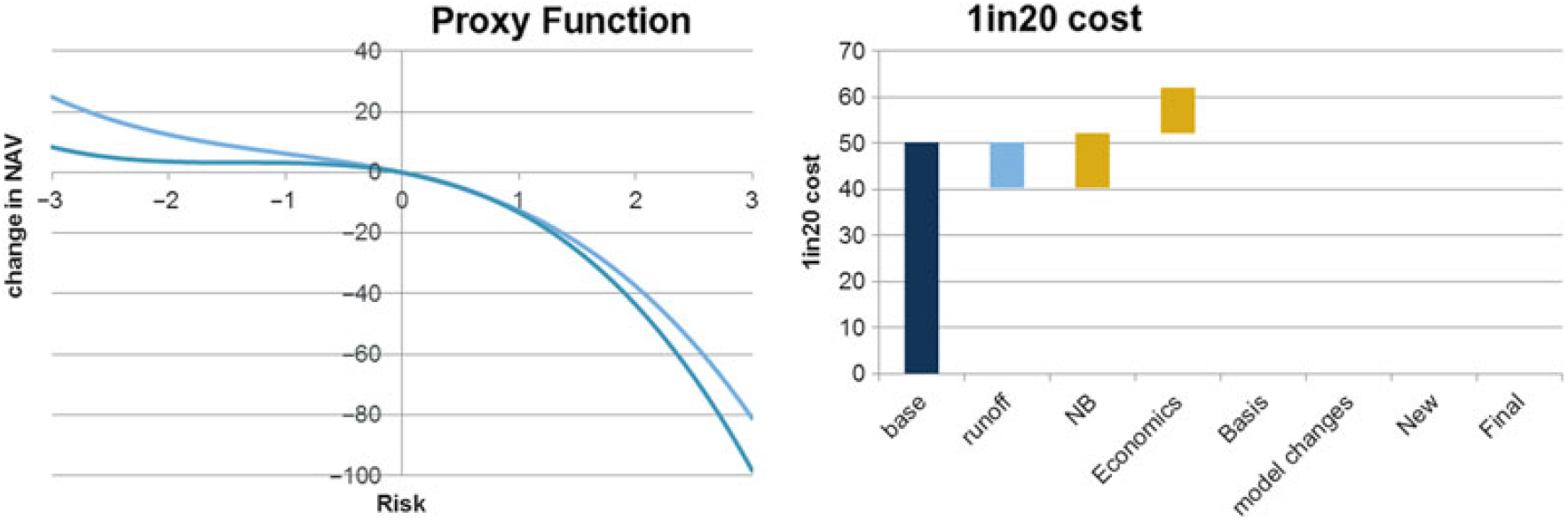
The roll forward process described in section 5 is used to re-state the proxy function to reflect changes in economic conditions.
Allow for Basis changes
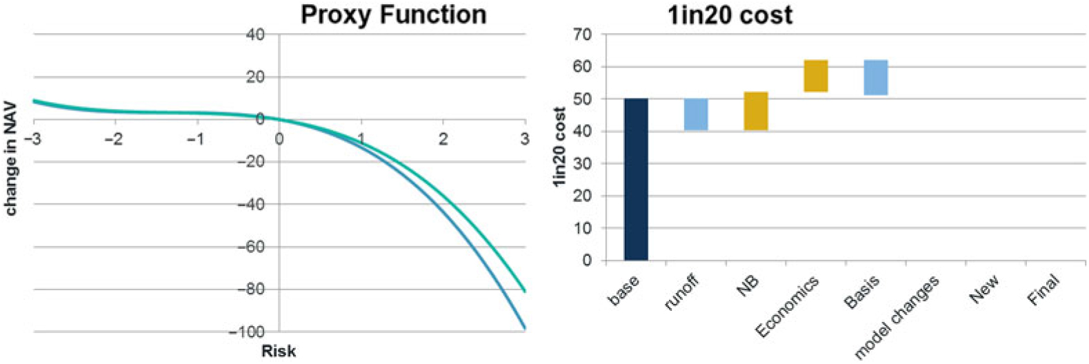
The proxy function is then re-stated to allow for basis changes.
Model changes
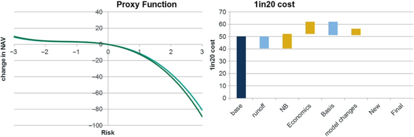
Model changes may be allowed for through scaling factors calibrated to estimate the size of the change.
Recalibrated proxy function

12.2.11 The results demonstrate how the evolution of the proxy function through each step may be analysed. The roll forward difference in the recalibration step gives a measure of the accuracy of the full process. Should any significant differences occur they should be investigated with a view to making future improvements. The improvement may be required to the proxy functions, the roll forward process or even the model structure (e.g. a new risk may be required).
12.2.12 The roll forward process for the proxy models may form part of a wider AoC process for the stochastic model. For example, by rerunning the full stochastic balance sheet model for each of the roll forward steps and also including steps for changes in the risk model and model structure, a full AoC on the stochastic model results (e.g. for metrics like the 1-in-X risk appetite or ruin probability) can be obtained.
12.2.13 In addition to using the roll forward cycle on the main proxy function elements, it should be used on any separate models of the discount rates features (e.g. the VA, the MA and the IAS19 discount rates). The roll forward cycle can be used to support any key judgement areas of the model. For example, if a firm requires a realistic model of how the IAS19 discount rates move under credit stress, being able to support the model behaviour through a track record in the roll forwards cycle is of great benefit.
12.3 Projections
12.3.1 This section discusses the use of projections to be used to estimate risk appetite 1-in-X amounts and ruin probabilities at future dates.
12.3.2 The projections discussed in this section take the form of a deterministic projection to a future time step. At that future time step the full balance sheet model is applied over its normal 1-year time frame. It should be noted that this form of model may not be suitable for the calculation of results such as the probability of ruin over a time frame. To derive such results a nested stochastic approach is required rather than a deterministic projection with a stochastic run at the end of the projection.
12.3.3 Projection of the proxy model may be used to investigate the suitability of a firm’s future business plan and ensure that it is sufficiently robust to withstand risk events. The following graph is used to illustrate how the results may be shown. In this case the gold lines show the areas the surplus may move to under a 1-in-25 event.
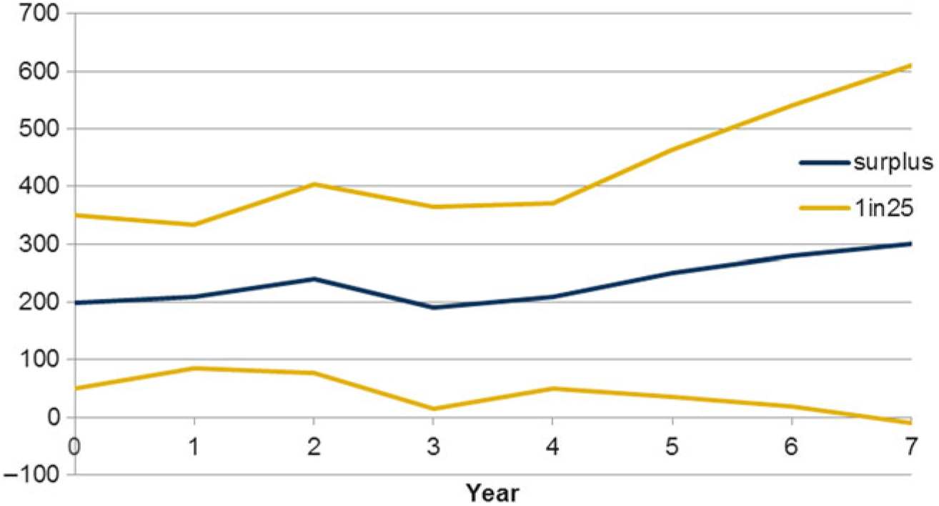
12.3.4 Using analysis such as this, a firm may be able to review and develop its business strategy in order that the surplus projections show a sustainable level that is also sufficiently robust.
12.3.5 In order to be able to simulate surplus movements at any future time step, we effectively need to be able to calibrate a proxy function with a time element. That is, we need to calibrate a function of the form:
Change in NAV = f(x 1, x 2, x 3, x n, time)
Where x i represents changes in risk i.
12.3.6 An approach to calibrate such a function would be to include the time element within the calibration set (and OOS set) and to fit as normal, projecting individual assets and liabilities where necessary. However, this may give rise to considerable practical difficulties. For this reason, a simpler approach may be to use a risk driver method.
12.3.7 A risk driver method uses drivers such as the BEL, sum assumed or expenses to approximate the run-off for different parts of the loss function. Separate drivers would need to be specified for different products and risks. An approximate approach is required to allow for cross terms.
12.3.8 A further consideration for long-term projections is the allowance for future new business. New business may be allowed for through an approach such as deriving a proxy function to represent the previous year’s new business for each product. The new business proxy functions then may be scaled for planned new business volumes. The projections need to take account of each cohort of future new business and the rate at which it would be expected to run off.
13. Conclusions
13.1 Purpose
13.1.1 This section concludes the analysis carried out with a summary of the key points identified and discusses the limitations of the model.
13.2 Summary
13.2.1 This paper has demonstrated a number of the techniques that may be used to produce a stochastic full balance sheet model. The key points from this paper can be summarised as follows:
• Understanding the robustness or stability of a firm’s balance sheet is a key element of firm’s risk management framework.
• It is likely to be a fundamental part of a firm’s risk appetite framework.
• To effectively model these elements, a stochastic full balance sheet model is required.
• The model should represent fully realistic views, and include elements such as the SCR and RM.
• The model needs to give a realistic allowance for changes in key discount rate features such as VA.
• The use of MLRE to focus on actual events may be more beneficial than standard Euler allocations.
• It is important to have a comprehensive framework around the proxy model that includes the roll forward and projection processes.
The outputs from the model may be used to develop risk mitigation strategies such as hedging or reinsurance. The specific events identified through the use of MLRE may be used in “war-gaming” exercises in which business experts consider the effects of a scenario and the most suitable response.
13.3 Limitations
13.3.1 This paper concludes by discussing the limitations around the model as this is a key aspect of any model.
13.3.2 The first aspect of the model limitations concerns the type of risks that are not included in the model. Some key examples of these are as follows:
• The risk of unforeseen regulatory changes affecting the balance sheet
• Risks associated with the business strategy
• Risks associated with gaining low margins in a difficult commercial environment
• Reputational risks
• Liquidity risks
13.3.3 These types of risks represent a very real threat to the stability of the projected balance sheet. However, they are not well suited to a model such as this. To allow for such risks, it is better to consider how they may take effect and what can be done in response to them through workshops with business experts.
13.3.4 A further key model limitation is with regard to proxy fitting itself. Of course, any proxy model is just an approximation to the full models and so will be subject to an element of error (quantified by the validation process). The models will also only be accurate within the risk space they are calibrated and validated over. A roll forward process is an approximate way of bringing proxy functions up to date.
13.3.5 The use of proxy models projected several years into the future should be treated with care. This approach generally relies on scaling different elements of the proxy function using drivers. Risk drivers are a standard technique used in the industry to represent the run-off of business, but the true run-off of business is often different from any driver.
13.3.6 The risk model used by any insurer is a further source of model limitation. It is well known that the calibration of risk models for use in a firm’s SCRs contains significant challenge as it is difficult to identify reliable data sets, representative of modern markets (or demographics), that have a sufficient number of years of data. Of particular difficulty is the selection and parameterisation of a copula for use in risk aggregation.
13.3.7 The use of a model with a 1-year time frame should be considered as an important limitation. A key example of the significance of this is for longevity trend risk. It is unlikely that, over a 1-year time frame, there could be mortality data or any event such as a medical breakthrough that would cause a large re-statement of firm’s allowance for longevity trend risk in their bases. However, it is entirely possible that such a change may take place over a number of years.
13.3.8 Finally the use of a single period model based on copula simulations should also be considered as a model limitation. The use of continuous time series models of market risk as are used with an ESG may give greater insight into the way in which market risks behave. These take into account economic theory to model the causal effects of one risk changing another rather than simply allowing for the statistical relationship between risks as within copula simulation models.
Acknowledgements
The authors would also like to thank the scrutineers of the paper for their helpful and detailed comments.
Appendix A: – Discussion of why the sf isn’t consistent with any risk distribution
The underlying assumptions in the SF are set out by EIOPA in EIOPA-14-322, 25 July 2014.
The underlying assumptions for the overall structure of the standard formula can be summarised as follows:
• Diversification effects are taken into account when capital requirements are aggregated by using correlation matrices. For aggregating the individual risk sub-modules and modules to obtain the overall SCR, linear correlation techniques are applied. The setting of the correlation coefficients is intended to reflect potential dependencies in the tail of the distributions, as well as the stability of any correlation assumption under stress conditions.
The underlying assumptions for the correlations in the standard formula can be summarised as follows:
• The dependence between risks can be fully captured by using a linear correlation coefficient approach.
• Due to imperfections that are identified with this aggregation formula (e.g. cases of tail dependencies and skewed distributions) the correlation parameters are chosen in such a way as to achieve the best approximation of the 99.5 % VaR for the overall (aggregated) capital requirement.
In summary, EIOPA states that correlation matrices are used for aggregation (a variance covariance formula approach is used). EIOPA recognises that this formula has limitations associated with it and states that the correlation parameters are chosen to allow for these.
It should be noted the EIOPA does not specify what the underlying risk model and loss function is. It would be expected that these need to exist if the correlation parameters were to be effectively changed so that the formula gives a result approximately equal to the true 99.5% VaR discussed above.
Where a variance covariance formula with a single stage is used, the formula is correct under three simplifying assumptions
• That the joint risk distribution is elliptical
• That individual risk losses are linear
• That combined risk losses are equal to the sum of the individual losses
The most well-known elliptical distribution is the multivariate normal. For this reason, where the variance covariance formula is used, it is common to implicitly assume that the joint risk distribution is normal (strictly speaking it could be from any elliptical distribution).
In contrast, where a variance covariance formula is used in a modular structure such as that used in the SF, the formula is not actually correct under any assumptions for the risk distribution and losses.
Therefore, the SF may be regarded as simply a formula rather than a true group model.
A demonstration that the SII aggregation structure is inconsistent with any risk distribution can be found in On a capital allocation principle coherent with the solvency 2 standard formula (Baione et al., Reference Baione, De Angelis and Granito2016).
Appendix B: – Mortality table used in example model

Appendix C: – Eigenvalues and eigenvectors used in the pca

The values here have been derived from a PCA of spot changes in the UK yield curve using data post the independence of the Bank of England in 1997. The results depend on the time period used, the data frequency and the “term buckets” (integer terms up to 25 years in this case). Reference 1 gives a detailed description of PCA.

 Open access