A) Checkerboard artifacts in CNNs

In CNNs, it is well-known that checkerboard artifacts are caused by two processes: forward-propagation of upsampling layers and backpropagation of convolutional layers. This paper focuses on these two issues in CNNs [Reference Odena, Dumoulin and Olah9,Reference Aitken, Ledig, Theis, Caballero, Wang and Shi14,Reference Sugawara, Shiota and Kiya21].

When CNNs include upsampling layers, there is a possibility that they will generate checkerboard artifacts, which is the first issue, referred to as issue A. Deconvolution [Reference Vincent and Francesco22,Reference Shi, Caballero, Theis, Huszar, Aitken and Ledig23], sub-pixel convolution [Reference Shi11], and resize convolution [Reference Odena, Dumoulin and Olah9] layers are well-known to include upsampling layers, respectively. Deconvolution layers have many names, including fractionally-strided convolutional layer and transposed convolutional layer, as described in [Reference Shi, Caballero, Theis, Huszar, Aitken and Ledig23]. In this paper, the term “Deconvolution” has the same meaning as others.

Checkerboard artifacts are also generated by the backward pass of convolutional layers, which is the second issue, referred to as issue B. We will mainly consider issue A in the following discussion, since issue B is reduced to issue A under some conditions.

B) SR methods using CNNs

SR methods using CNNs are classified into two classes as shown in Fig. 1. Interpolation-based methods [Reference Dong, Loy, He and Tang6,Reference Dong, Loy, He and Tang24–Reference Tai, Yang and Liu27], referred to as “class A,” do not generate any checkerboard artifacts in CNNs, due to the use of an interpolated image as an input to a network. In other words, CNNs in this class do not have any upsampling layers.

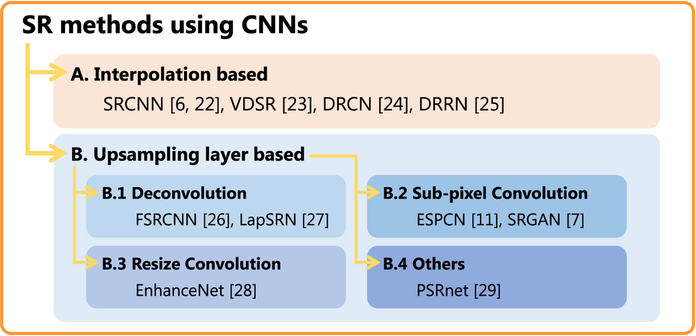
Fig. 1. Classification of SR methods using CNNs. There is a possibility that SR methods will generate checkerboard artifacts, when CNNs include upsampling layers.

When CNNs include upsampling layers, there is a possibility that CNNs will generate checkerboard artifacts. This class, called “class B” in this paper, has provided numerous excellent SR methods [Reference Ledig7,Reference Shi11,Reference Dong, Loy and Tang28–Reference Sugawara, Shiota and Kiya33] that can be executed faster than those in class A. Class B is also classified into a number of sub-classes according to the type of upsampling layer. This paper focuses on class B.

CNNs are illustrated in Fig. 2 for an SR problem, as in [Reference Shi11], where the CNNs consist of two convolutional layers and one upsampling layer. I _LR and $f_c^{(l)}(I_{LR})$ are a low-resolution (LR) image and c-th channel feature map at layer l, and f(I _LR) is an output of the network. The two layers have learnable weights, biases, and ReLU as an activation function, where the weight at layer l has K _l × K _l as a spatial size and N _l as the number of feature maps.

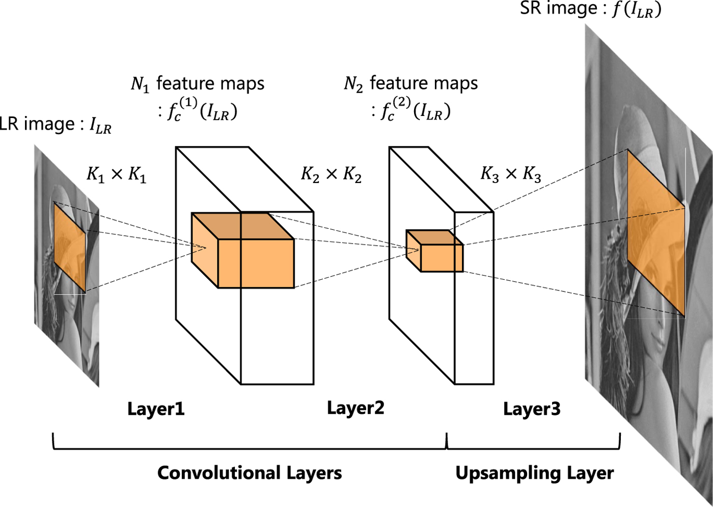
Fig. 2. CNNs with an upsampling Layer.

There are numerous algorithms for computing upsampling layers, such as deconvolution [Reference Vincent and Francesco22,Reference Shi, Caballero, Theis, Huszar, Aitken and Ledig23], sub-pixel convolution [Reference Shi11], and resize convolution [Reference Odena, Dumoulin and Olah9] ones, which are widely used in typical CNNs. In addition, recently, some excellent SR methods have been proposed [Reference Zhang, Zuo and Zhang31,Reference Zhang, Li, Li, Wang, Zhong and Fu34].

C) Works related to checkerboard artifacts

Checkerboard artifacts have been discussed by researchers for designing multirate systems including filter banks and wavelets [Reference Harada, Muramatsu and Kiya17–Reference Iwai, Iwahashi and Kiya20]. However, most research has been limited to cases of using linear systems, so it cannot be directly applied to CNNs due to the non-linearity of CNNs. Some pieces of works related to checkerboard artifacts for linear systems are summarized, here.

It is known that linear interpolators, which consist of up-samplers and linear time-invariant systems, cause checkerboard artifacts due to their periodic time-variant property [Reference Harada, Muramatsu and Kiya17–Reference Harada, Muramatu and Kiya19]. Figure 3 illustrates a linear interpolator with an up-sampler ↑ U and a linear time-invariant system H(z), where positive integer U is an upscaling factor and H(z) is the z transformation of an impulse response. The interpolator in Fig. 3(a) can be equivalently represented as a polyphase structure as shown in Fig. 3(b). The relationship between H(z) and R _i(z) is given by

(1)$$H(z) = \sum_{i=1}^{U}R_{i}(z^{U})z^{-(U-i)},$$

where R _i(z) is often referred to as a polyphase filter of the filter H(z).

Fig. 3. Linear interpolators with upscaling factor U. (a) General structure, (b) polyphase structure.

The necessary and sufficient condition for avoiding checkerboard artifacts in the system is shown as

(2)$$R_{1}(1) = R_{2}(1) = \cdots = R_{U}(1) = G.$$

This condition means that all polyphase filters have the same DC value, i.e. a constant G [Reference Harada, Muramatsu and Kiya17–Reference Harada, Muramatu and Kiya19]. Note that each DC value R _i(1) corresponds to the steady-state value of the unit step response in each polyphase filter R _i(z). In addition, the condition of equation (2) can be also expressed as

(3)$$ H(z) = P(z)H_0(z),$$

where,

(4)$$ H_0(z) = \sum_{i=0}^{U-1} z^{-i},$$

and H ₀(z) and P(z) are an interpolation kernel of the zero-order hold with factor U and a time-invariant filter, respectively. Therefore, a linear interpolator with factor U does not generate any checkerboard artifacts, when H(z) includes H ₀(z). In the case without checkerboard artifacts, the step response of the linear system has a steady-state value G as shown in Fig. 3(a). Meanwhile, the step response of the linear system has a periodic steady-state signal with the period of U, such as R ₁(1), …, R _U(1), if equation (3) is not satisfied.

To intermediate between signal processing field and computer vision one, the correspondence relation of some technical terms is summarized in Table 1.

Table 1. Correspondence relation of technical terms in signal processing and computer vision

A) CNNs with upsampling layers

We focus on upsampling layers in CNNs, for which there are numerous algorithms such as deconvolution [Reference Vincent and Francesco22,Reference Shi, Caballero, Theis, Huszar, Aitken and Ledig23], sub-pixel convolution [Reference Shi11], and resize convolution [Reference Odena, Dumoulin and Olah9]. For simplicity, one-dimensional CNNs will be considered in the following discussion.

It is well-known that deconvolution layers with non-unit strides cause checkerboard artifacts [Reference Odena, Dumoulin and Olah9]. Figure 4 illustrates a system representation of deconvolution layers [Reference Vincent and Francesco22,Reference Shi, Caballero, Theis, Huszar, Aitken and Ledig23] that consist of interpolators, where H _c and b are a weight and a bias in which c is a channel index, respectively. The deconvolution layer in Fig. 4(a) can be equivalently represented as a polyphase structure in Fig. 4(b), where R _c,n is a polyphase filter of the filter H _c in which n is a filter index. This is a non-linear system due to the bias b.

Fig. 4. Deconvolution layer [Reference Vincent and Francesco22,Reference Shi, Caballero, Theis, Huszar, Aitken and Ledig23]. (a) General structure, (b) Polyphase structure.

Figure 5 illustrates sub-pixel convolution layers [Reference Shi11], where R _c,n and b _n are a weight and a bias, and $f_n^{\prime }(I_{LR})$ is an intermediate feature map in channel n. Comparing Fig. 4(b) with Fig. 5, we can see that the polyphase structure in Fig. 4(b) is a special case of the sub-pixel convolution layers in Fig. 5. In other words, Fig. 5 is reduced to Fig. 4(b), when satisfying b ₁ = b ₂ = · · · = b _U. Therefore, we will focus on sub-pixel convolution layers as a general case of upsampling layers to discuss checkerboard artifacts in CNNs.

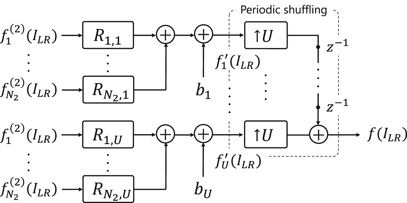
Fig. 5. Sub-pixel convolution layer [Reference Shi11].

B) Checkerboard artifacts in upsampling layers

Let us consider the unit step response in CNNs. In Fig. 2, when the input I _LR is the unit step signal I _step, the steady-state value of the c-th channel feature map in layer 2 is given as

(5)$$ \hat{f}_c^{(2)}(I_{step}) = A_c,$$

where A _c is a positive constant value that is decided by filters, biases, and ReLU. Therefore, from Fig. 5, the steady-state value of the n-th channel intermediate feature map is given by, for sub-pixel convolution layers,

(6)$$ \hat{f}_n^{\prime}(I_{step}) = \sum_{c=1}^{N_2} \, A_c \overline{R}_{c,n} + b_n,$$

where $\overline {R}_{c,n}$ is the DC value of the filter R _c,n.

Generally, the condition, which corresponds to equation (2) for linear multirate systems,

(7)$$ \hat{f}_1^{\prime}(I_{step}) = \hat{f}_2^{\prime}(I_{step}) = \cdots = \hat{f}_U^{\prime}(I_{step})$$

is not satisfied, so the unit step response f(I _step) has a periodic steady-state signal with the period of U. To avoid checkerboard artifacts, equation (7) has to be satisfied, as well as for linear multirate systems.

C) Upsampling layers without checkerboard artifacts

To avoid checkerboard artifacts, CNNs must have the non-periodic steady-state value in the unit step response. From equations (6), equation (7) is satisfied if

(8)$$ \overline{R}_{c,1} = \overline{R}_{c,2} = \cdots = \overline{R}_{c,U}, \, c = 1, 2, \ldots, N_{2}$$

(9)$$ b_{1} = b_{2} = \cdots = b_{U}.$$

Note that, in this case,

(10)$$ \hat{f}_1^{\prime}(K \cdot I_{step}) = \hat{f}_2^{\prime}(K \cdot I_{step}) = \cdots = \hat{f}_U^{\prime}(K \cdot I_{step})$$

is also satisfied, where K is an arbitrary constant value. However, even when each filter H _c in Fig. 5 satisfies equation (2) or equation (3), equation (9) is not met, but equation (8) is met. Both equations, i.e., equations (8 and 9) have to be met to avoid checkerboard artifacts in CNNs. Therefore, we have to find a novel way of avoiding checkerboard artifacts in CNNs. Note that equations (5) and (7) correspond to values in case that the input I _LR is the unit step I _step. Therefore, other general inputs, the output feature map would not be the same even when equations (5) and (7) are met.

In this paper, we propose adding the kernel of the zero-order hold with factor U, i.e., H ₀ in equation (4), after upsampling layers, as shown in Fig. 6. In this structure, the unit-step response outputted from H ₀ have constant value as the steady state values, even when an arbitrary periodic signal with a period of U is inputted to H ₀. As a result, Fig. 6 can satisfy equation (7). In other words, the steady-state values of the step response are not periodic in this case.

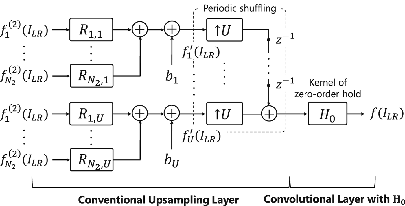
Fig. 6. Proposed upsampling layer structure without checkerboard artifacts. Kernel of zero-order hold with factor U is added after upsampling layers.

The difference between the conventional upsampling layers and the proposed structure is whether the structure has H ₀ forcibly inserted for avoiding checkerboard artifacts or not. The operation of sub-pixel convolution and deconvolution layers can be interpreted as a combination of upsampling and convolution, where upsampling corresponds to the operation that is to insert (U − 1) zeros between sample values. The conventional upsampling layers do not include H ₀ generally unless forcibly inserting H ₀ into convolution, so checkerboard artifacts are generated.

There are three approaches to using H ₀ in CNNs that differ in terms of how CNNs are trained as follows.

D) Checkerboard artifacts in gradients

It is well-known that checkerboard artifacts are also generated in gradients of convolutional layers [Reference Odena, Dumoulin and Olah9] since the operations of deconvolution layers are carried out on the backward pass to compute the gradients. Therefore, both approaches 2 and 3 can avoid checkerboard artifacts as well as for deconvolution layers. Note that, for approach 2, we have to add the kernel of the zero-order hold before convolutional layers to avoid checkerboard artifacts on the backward pass.

It is also well-known that max-pooling layers cause high-frequency artifacts in gradients [Reference Odena, Dumoulin and Olah9]. However, these artifacts are generally different from checkerboard artifacts, so this paper does not consider these high-frequency artifacts.

A) Super-resolution

The proposed structure without checkerboard artifacts was applied to the SR methods using deconvolution and sub-pixel convolution layers. The experiments with CNNs were carried out under two loss functions: mean squared error (MSE) and perceptual loss.

2) Training details

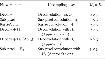
Table 2 illustrates the CNNs used in the experiments, which were carried out on the basis of the CNNs in Fig. 2. For the other two layers in Fig. 2, we set (K ₁,  N ₁) = (5,  64), (K ₂,  N ₂) = (3,  32) as in [Reference Shi11]. In addition, all networks were trained to minimize the MSE ${1}/{2} \Vert I_{HR}-f(I_{LR}) \Vert^{2}$ and the perceptual loss 1/2‖ϕ(I _HR) − ϕ(f(I _LR))‖² averaged over the training set, where ϕ calculates feature maps at the fourth layer of a pre-trained VGG-16 model as in [Reference Johnson, Alahi and Li13]. Note that $\hbox {Deconv}+{\rm H}_0$, $\hbox {Deconv}+{\rm H}_0$ (Ap. 3), and $\hbox {Sub-pixel}+ {\rm H}_0$ in Table 2 use the proposed structure.

Table 2. CNNs used for super-resolution tasks

For training, Adam [Reference Kingma and Ba38] with β ₁ = 0.9,  β ₂ = 0.999 was employed as an optimizer. In addition, we set the batch size to 4 and the learning rate to 0.0001. The weights were initialized with the method described in He et al. [Reference He, Zhang, Ren and Sun39]. We trained all models for 200 K iterations. All models were implemented by using the TensorFlow framework [Reference Abadi, Agarwal and Barham40].

3) Experimental results

Figure 7 shows examples of SR images generated under perceptual loss, where mean PSNR values for each dataset are also illustrated. In this figure, (b) and (f) include checkerboard artifacts, and (c)–(e), (g)–(i) do not. Moreover, it is shown that the quality of SR images was significantly improved by avoiding the artifacts. Approaches 2 and 3 also provided better quality images than approach 1. Note that ResizeConv did not generate any artifacts, because it uses a pre-defined interpolation like in [Reference Dong, Loy, He and Tang6]. In Fig. 8, the usefulness of the proposed avoidance condition is demonstrated. It was confirmed that CNNs generated checkerboard artifacts under the conventional condition unless CNNs satisfied the proposed condition. Figure 9 shows other examples of SR images. In Fig. 9, the trend is almost the same as that in Fig. 7.

Fig. 7. Experimental results of super-resolution imaging under perceptual loss [PSNR(dB)]. (b) and (f) include checkerboard artifacts, and (c), (d), (e), (g), (h), and (i) do not.

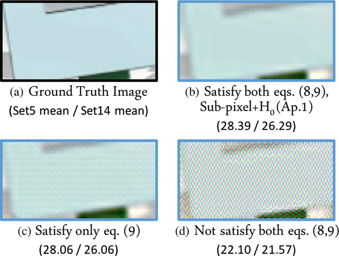
Fig. 8. Super-resolution imaging using perceptual loss under various avoidance conditions [PSNR(dB)] (sub-pixel convolution).

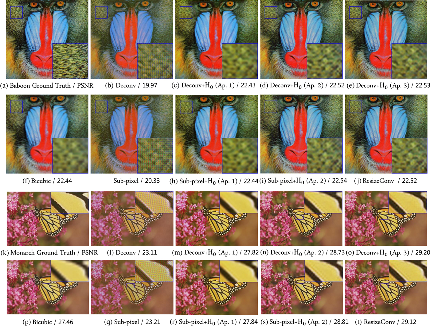
Fig. 9. Super-resolution examples of “Baboon” and “Monarch” under perceptual loss. PSNR values are illustrated under each sub-figure. (b), (g), (l), and (q) include checkerboard artifacts, and other examples do not.

Table 3 illustrates the average execution time when each CNNs were run 10 times for some images in Set14. Resize-Conv has the highest computational cost in this table, although it did not generate any checkerboard artifacts. From this table, the proposed approaches have much lower computational costs than with resize convolution layers. Note that the results were obtained on a PC with a 3.30-GHz CPU and a main memory size of 16 GB.

Table 3. Execution time of super-resolution (sec)

4) Loss functions

It is well-known that perceptual loss results in sharper SR images despite lower PSNR values [Reference Johnson, Alahi and Li13,Reference Sajjadi, Schölkopf and Hirsch30], and it generates checkerboard artifacts more frequently than under MSE loss as described in [Reference Odena, Dumoulin and Olah9,Reference Johnson, Alahi and Li13,Reference Aitken, Ledig, Theis, Caballero, Wang and Shi14,Reference Blau and Michaeli41]. In Fig. 10, which demonstrates artifacts under MSE loss, (b) and (f) also include checkerboard artifacts as well as in Fig. 7, although the distortion is not that large, compared with under perceptual loss. There is a possibility that any loss function causes checkerboard artifacts, but the magnitude of checkerboard artifacts depends on a class of loss functions used for training networks. The proposed avoidance condition is useful under any loss function.

Fig. 10. Experimental results of super-resolution under MSE loss [PSNR(dB)]. (b) and (f) also include checkerboard artifacts as well as in Fig. 7, although the distortion was not that large, compared with under perceptual loss.

B) Image classification

Next, the proposed structure without checkerboard artifacts was applied to CNNs-based image classification models.

2) Training details

Table 4 illustrates the CNNs used in the experiments, which were run on the basis of ResNet-110 [Reference He, Zhang, Ren and Sun2]. Note that the projection shortcut [Reference He, Zhang, Ren and Sun2] was used only for increasing the number of dimensions, and all convolutional layers with a stride of 2 in ResNet-110 were replaced by downsampling layers in Table 4.

Table 4. CNNs used for image classification tasks

All of the networks were trained by using stochastic gradient descent with momentum for 300 epochs. The learning rate was initially set to 0.1, and decreased by a factor of 10 at 150 and 225 epochs. The weights were initialized by the method introduced in [Reference He, Zhang, Ren and Sun39]. We used a weight decay of 0.0001, a momentum of 0.9, and a batch size of 64.

3) Experimental results

Figure 11 shows examples of gradients, which were computed on the backward pass of the first downsampling layer, for each CNN. In this figure, (a) includes checkerboard artifacts, and (b) and (c) do not.

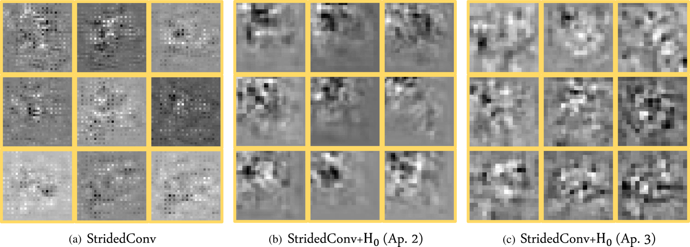
Fig. 11. Gradients computed in first downsampling layer. (a) includes checkerboard artifacts, and (b) and (c) do not.

The results for CIFAR10 and CIFAR100 are illustrated in Table 5, where “+” indicates the use of the standard data augmentation. It is shown that approach 3 performed the best in this table. This trend was almost the same for the SR tasks.

Table 5. Error rates on CIFAR10, CIFAR100 datasets (%)