Introduction
This paper is concerned with linearization techniques as a way of estimating the glaciological response to changes in the accumulation rate on ice sheets. That is, changes in the accumulation rate result in changes in ice-sheet geometry, which in turn produce changes in the movement of the ice. Linearized methods have, of course, some disadvantages in modelling the non-linear evolution equations for ice sheets, but also have advantages in that the model does not require specification of the rate factor in the viscous law. In this sense, the model is closer to the data than “matched” nonlinear models. Linearization techniques have previously been applied to modern ice sheets (e.g. Reference OerlemansOerlemans, 1981; Reference Hindmarsh and MorrisHindmarsh, 1992; Reference Drewry and MorrisDrewry and Morris, 1992; Reference Van der VeenVan der Veen, 1993), but these have only been of ordinary differential equations (zero-dimensional (0-D models). This paper presents the first computations of the normal modes of an observed ice sheet.
The disadvantages of this method relate principally to an inability to describe changes in ice-stream flow, which is expected to be turn-linear. The disadvantage is more apparent than real, as research methods remain far from creating adequate models of basal and lateral processes in ice streams, and models of ice streams, incorporating what are believed to be the relevant dynamical features, can only provide conjectural prognoses.
The advantages of linearized techniques relate to ease of use for non-glaciologists, and the fact that no model tuning is necessary. That is, in non-linear models (e.g. Reference HuybrechtsHuybrechts, 1992) the accumulation rate and the viscous properties are parameterized and tuned in order to obtain a good fit between observed and computed heights. This was an appropriate response a few years ago, but the progress of satellite altimctry since then (Reference Bamber and HuybrechtsBamber and Huybrechts, 1996) has made ice-sheet elevation the most accurately known of all the ice-sheet descriptors. Linearization methods permit prognostic calculations to be made without knowing the rate factor, as the rate equation stems ultimately from the mass accumulation. Thus, no tuning is necessary and computations of ice-sheet geometry evolution can be compared directly with observations.
Moreover, a practical consequence is that no estimate is required of slow changes in response to, for example, the end of the Last Ice Age before the response to changes in forcing can be estimated. One aim ofthe work described here is the production of ice-sheet models describing a short-term response that can be used in models of other parts of the climate system.
It should be emphasized that linearized models are rational approximations — that is, they come equipped with their own error bars. For small perturbations, linearized methods are accurate and the order of magnitude of the error term can be computed.
The paper will discuss issues of normal mode initialization and spaiial filtering of data. The non-linear ice-sheet equations and their linearizaiions in two horizontal dimensions (2HD), are reviewed and compared to results from the non-linear Eismint Benchmark (Reference Huybrechts and PayneHuybrechts and others, 1996). Finally, the modes of a real 2HD ire sheet (the Antarctic ice sheet) are computed.
Normal Mode Initializations of Ice Sheets
Normal modes are the eigcnfunctions and eigenvalues that ensue from selling up a linear(ized) model and solving a related eigenvalue problem. The “normal” pertains to the canonical nature of these modes. Each mode has an associated e-folding time constant, and the spatial structure of each mode is different. Essentially, shorter spatial-length scales are expected to relax faster (have a shorter e-folding time constant).
Normal modes are widely used in geophysics and geophysical fluid dynamics. Despite being a classical technique, they have not been used widely in glaeiology. An important use in meteorology has been the filtering of meteorological data in order to initialize models with data that do not excite non-physical numerical modes.
As explained above, ice-sheet-model geometry, when compared to real data, represents a trade-off between the tuning of the rate factor and the parameterization of the accumulation-rate distribution. An obvious issue is whether normal mode techniques can be exploited to initialize ice-sheet models. In particular, the advent of satellite altimetry has produced very accurate elevation data that need to be included in ice-sheet models if dynamics are to be inferred from observations.
When observed elevations are used in non-linear ice-sheet models, it is found that smaller-scale structure is relaxed out quickly, sometimes causing numerical problems (Reference Oerlemans and van der VeenOerlemans and Van der Veen, 1984). Current observations of basal topograph) are nowhere near the same plan-view resolution, meaning that errors in the thickness cause computed and spurious ice-flow anomalies, resulting in the numerical smoothing described above.
An obvious question is whether normal-mode initialization techniques can be used in some form in ice-sheet modelling, with the specific objective of ensuring that observations are used as an initial state, rather than some trade-off between ignorance of accumulation, rate factor, ice-sheet thickness and the need to maintain numerical stability.
Because the ice-sheet equation represents an initial value problem, any measured data are physically consistent. Anomalous roughness and topographic sinks (e.g. the Vostok depression) could simply be relaxing out. Under an assumption of steady state, the origin of many features becomes more problematical, but can still, in principle, be explained by local variations in the poorly known basal topography or, in a more contived way, by local variations in the rate factors for internal deformation or for sliding. Topographic depressions can arise as a result of locally enhanced basal melting, or may conceivably occur as a result of “Stokes effects” where, for example, small-scale variations in the basal topography result in local failure of the shallow-ice approximation (e.g. Reference JóhannessonJóhannesson, 1992).
Small-scale (wavelength of a few gridcells) surface roughness, that is not reflected in causatory variation in the rate factor or the basal topography, is relaxed out by the action of non-linear solutions. Balance-flux calculations and ensuing linearizations are not affected by this problem provided topographic depressions are dealt with by selling basal melting to be larger than the accumulation.
Such noisy data can be dealt with in several ways when initializing models:
-
(a) Accept the data as a valid zeroth-order approximation and compute a set of eigenfunctions and eigenvalues. It could transpire that even the low wave-number eigenfunctions are noisy.
-
(b) Smooth heuristically and compute the normal modes.
-
(c) Select a smooth zeroth-order solution on an error minimization criierion and compute the normal modes (Reference HindmarshHindmarsh, in press).
In the latter two cases there will be a residual between the zeroth-order solution and the date. This can be reduced by fitting the residual with the normal modes: this is a normal mode initialization as commonly used in other geosciences (e.g. Reference DaleyDaley, 1992). The more modes used, the smaller the wavelength of feature that can be modelled. The remaining variation is filtered by using functions that have a close relation to ice-sheet physics rather than by an arbitrary smoothing.
Clearly, if option a produces smooth normal modes, then it is the simplest option. Provided sink-holes are eliminated from the observed data, then the computed normal modes do not appear noisy. It is possible that holes could be reconstituted by using the normal modes, but testing the efficacy of this technique is outside the immediate aims of this paper. We shall see that option (a) is possible.
The Ice-Sheet Equation and Its Linearizations
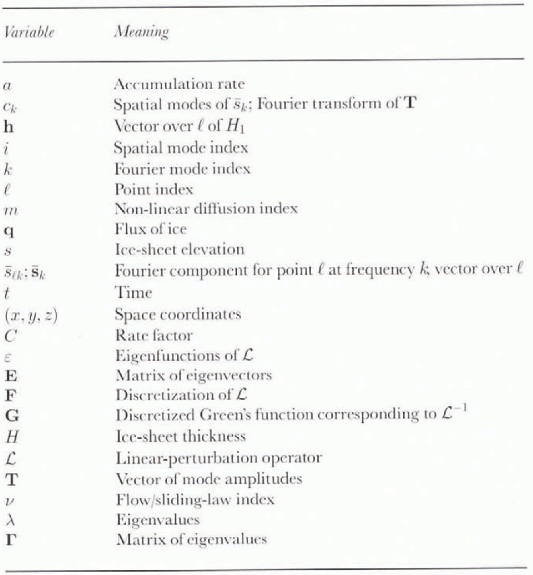
Notation is summarized in Table 1. When considering the mechanics of ice sheets a reduced model is normally used (Reference HutterHutter, 1983; Reference MorlandMorland, 1984; Reference FowlerFowler, 1992), obtained from a scaling of the Stokes equations. The scaling yields simple functional forms for the vertical variation of the stress field and a considerable computational saving. Further manipulation of the reduced model results in the ice-sheet equation:
where H(x, y, t) is the thickness of the ice sheet, s(x, y, t) is the upper surface and a is the surface mass-balance exchange. Boundary conditions for this model are:
where y = V(x), the prescribed margin. This corresponds to the Vialov-Nye calving condition, where the ire thickness at the margin is less than the maximum thickness. More advanced models, to be considered in future work, would have non-zero thickness at the grounding line and a moving grounding line. This has already been treated in a linearized fashion for one horizontal dimension (1HD) by Reference HindmarshHindmarsh (1996a).
Table 1. Notation
These evolution equations describe the evolution of ice-sheet thickness where the flow mechanism is either internal deformation according to a non-linearly viscous flow law or sliding according to a Weeriman-type law. The analyses carried out in this paper are not limited to these situations.
The quantity C is directly related to either a weighted
vertical average rate factor
![]() defined below in Equation (6) of the rale factor A
d used in the viscous relationship:
defined below in Equation (6) of the rale factor A
d used in the viscous relationship:
where E is a second invariant of the deformation rale and τ is a second invariant of the deviator stress (Reference GlenGlen, 1955) or comes from a sliding relation of the form:
(Reference WeertmanWeertman, 1957). We construct the following quantities for use in the general evolution equation:

The derivation of the evolution Equation (1) using the shallow-ice approximation is standard (Reference HutterHutter, 1983; Reference MorlandMorland, 1984; Reference FowlerFowler, 1992). A futher standard derivation, which, in the present notation, can be found in Reference HindmarshHindmarsh (1996a) yields a formula for the ice flux q:
where:

If instead we are dealing with sliding, then:
and use of the continuity equation:
results in the non-linear diffusion type Equation (1). Linearizations are computed by expanding H and a in a series

and truncating at first order. The Taylor expansion of qx , for example, yields:

Specifically, we can compute:

and we can see that the zeroth order and first-Order equations are:

Boundary conditions are the crude approximation of fixing the elevation at the margin of the ice sheet. Moving boundaries can be incorporated into linearizations (Reference HindmarshHindmarsh, 1996a) but the technical difficulties of extending this approach to two horizontal dimensions mean that it is worth investigating the fixed margin problem first in order to assess the potential of linearization techniques. Ablating margins are not considered in this paper.
The zeroth-order solution can be identified with the long-term trend (e.g. the response to pre-industrial climate conditions) and the first-order solution with the faster response to perturbation. The long-term trend could of course be steady state. If the technique were being applied rigorously time should be expanded in two time-scales, but the complexities of the required notation outweigh the benefits, so the procedure is justified heuristirally by saving that the perturbation is expected to grow over time-scales where the zeroth-order solution hardly changes, and a “snap-shot” can be taken of the profile to compute the coefficients in Equation (9)
The curious way of writing the zeroth-order equation is to emphasize that ignorance of accumulation rate and rate of change of surface profile have exactly the same significance. It is assumed that a 1 is known, in the sense that the response to a postulated change in the accumulation rate is being evaluated.
A significant feature of the perturbation equation is the absence of the rate factor in the first-order equation. The time dimension is introduced into the ice-sheet equation by the accumulation rate of snow and through the rate factor. In a strain-rate controlled flow, such as is assumed here, the ice sheet exists to discharge the snow fall, and the time-scales are set by meteorological factors. The ice-sheet geometry adjusts so as to set the theological time-scale equal to the meteorological time-scale. Where there are internal oscillations in the ice sheet, the fast and slow phases correspond to stress-controlled flows, and the perturbation equation will not apply. In any case, the perturbation equation is a linear equation and cannot have limit cycle solutions such as those described by Reference PaynePayne (1995).
By setting a 1 = 0 the linear equation can be put into homogeneous form. A separation of variables technique can be used to generate solutions to the homogeneous form using an eigenvalue expansion, which can subsequently be used to construct solutions to the inhomogeneous form. The theory is reviewed below. In general, the eigenproblem has to be solved numerically. There are potential problems associated with singular behaviour at the divide and margin.
(Reference HindmarshHindmarsh 1996b, Reference HindmarshIn press) has considered perturbations about the 1HD Vialov-Nye (VN) (Reference VialovVialov, 1958; Reference NyeNye, 1959), solution, which is computed by setting ∂tH = 0 and a = am0 , = C = Cm0 both constants, into the plane-flow version of Equation (1) and integrating the resulting ordinary differential equation (ODE). Reference HindmarshHindmarsh (in press) treated the singularities at margin and divide accurately by using Fobenius expansions (see also Reference FowlerFowler, 1992). In the 2HD calculations reported here, Taylor expansions are used at the margin and at the divide. Calculations for 1HD, based on the principles described below for 2HD, show that this makes very little difference to the computed eigenvalues or eigenfunctions. This presumably arises as a result of the robustness of Sturm-Liouville systems to model perturbation (Reference PrycePryce, 1993). Taylor, rather than Frobenius, expansions are almost universally used in ice-sheet modelling when the non-linear problem is treated.
Zeroth-Order Flux Computation Consistent with Finite-Difference Grids
Given that the perturbation procedure will be carried out on a finite-difference grid, it is highly desirable that the zeroth-order fluxes satisfy the conservation equation exactly. For this reason, efficient shooting procedures (Reference Budd and WarnerBudd and Warner, 1996; Reference Rémy, Ritz and BrissetRémy and others, 1996) are not used. The procedure is simply to compute the flux arriving at a gridpoint from x- and y-direction connections, compute the flux out using continuity, and divide it between all the outlet connections (i.e. to points at a lower elevation) in linear proportion to their slopes.
Consider the coefficient
. Then,
. Even though s 0 and H 0 are known, C is not, meaning that D is also unknown. A finite-difference approximation is:
for each of the outlet points, where Di is an unknown. The outlet discharges and D can be solved with the additional equation:

Balance flux calculations have been used by Reference Rémy, Ritz and BrissetRémy and others (1996) to solve for the rate factor and thence the basal temperature.
In practice, the grid-centred fluxes are computed by solving a set of linear
equations. These satisfy continuity exactly and also return the quantity
![]() . While the method is algorithmically different from that of
Reference Budd and WarnerBudd and Warner (1996), the two
methods seem to be consistent at O(Δ
x
). The purpose of using a different method is to ensure that the
continuity equation is respected exactly at zeroth order on the
finite-difference grid used to solve the eigenproblem.
. While the method is algorithmically different from that of
Reference Budd and WarnerBudd and Warner (1996), the two
methods seem to be consistent at O(Δ
x
). The purpose of using a different method is to ensure that the
continuity equation is respected exactly at zeroth order on the
finite-difference grid used to solve the eigenproblem.
The Eigenvalue Problem and its Discretization
The first-order perturbation Equations (10) and (11) are conveniently written in operator form:
H1(x,y,t) is written in a separable form:
and substitution of this into the homogeneous form of Equation (12) yields:

where λ is an eigenvalue. The spatial equation is:
which has eigenvalue solutions ε(x, y).
Now, in general it cannot be assumed that the eigenfunctions are orthogonal, and it is also convenient simply to consider eigenfunction expansions truncated after M terms, and to consider the eigenfunctions evaluated at M points: this is what emerges from solving the algebraic eigenvalue problem resulting from the discretization of the operator
, which is denoted by the matrix F. Suppose that R(x,y) is represented by M points sampled on the grid; these points have value rl l = (1, M). Then, the matrix representation of Equation (13) is:
where the diagonal entries of the matrix Λ are the eigenvalues. This is an algebraic eigenvalue problem Reference WilkinsonWilkinson, 1965), which is satisfied by M linearly independent eigenvectors. We construct a matrix E the ith column of which is the ith eigenvector evaluated at M points. Thus, i is an index of spatial mode number.
It will be assumed that these eigenfunctions are linearly independent and form a complete set — there have been no cases found where this is not true. It may thus be written that:

and, after using Equation (13) the perturbation Equation (12) becomes:
By sampling Equation (14) at M points, this equalion may be written as a discretized matrix equation:
where a is the vector of accumulation rate sampled at the M points. There are thus M linear equations corresponding to the M points of evaluation, and the elevations at the sampling points are given by:
where h is the vector of H1, l at the sampling points. By multiplying Equation (15) by E−1, the existence of which is assured by the fact that the eigenvectors are independent, M mode-evolution equations are obtained:
with the rows of the inverse eigenvector matrix playing the role of a modal weighting function in space for the accumulation rate. By definition F = EΛE−1.
At steady state, we have EΛT = −a. whence
where G = −F−1 plays a role analogous to a Green's function. A refinement is to suppose that N modes have sufficiently slow relaxation (small eigenvalues) that it is necessary to consider their dynamic values, while the remaining L = M-N modes are regarded as being in steady state. Then, a quantity h1, can be constructed which represents that part of the perturbation that relaxes sufficiently quickly to be in equilibrium with the instantaneous forcing. These are the so-called “slaved” modes, which are computed according to:
where colon (“Matlab”) notation is used in the subscripts (Reference Golub and van LoanGolub and Van Loan, 1989, p. 7). For example, the range of indices being considered are represented by a : b, with a single colon by convention representing the total range.
Here, GL can be regarded as the Green's function for the slaved modes. The evolution of the remaining N dynamic modes is given by
so that:
In practice, one often does not wish to compute the whole eigenvalue sequence, and it is a straightforward exercise to show that:
Thus, it is necessary to compute G, the matrix inverse of the operator matrix F, and those eigenvalues that relax sufficiently slowly that we are interested in their dynamics. Truncations of such generalised Fourier expansions of ice sheets have been considered by Reference HindmarshHindmarsh (1990), who concluded that computation of the evolution of a few dynamic modes represented the evolution of the ice sheet reasonably well.
In 1HD the first-order perturbation Equations (10) and (11) can be written in Sturm-Liouville form and solved using either finite-difference methods or shooting methods (Reference HindmarshHindmarsh, in press). The eigenfunctions are orthogonal. In 2HD, this is not true in general and the perturbation equation, which includes cross-derivative terms, is discrelized using a standard nine-point conservative stencil, which produces a sparse, non-symmetric matrix. The eigenvalue problem was solved using the ARPACK software (Reference SorensenSorensen, 1992) which deals specifically with large, sparse, non-symmetric problems. The software uses Arnoldi iteration (see e.g. Reference ChatelinChatelin, 1993), producing the “Ritz values”, which are approximations to the eigenvalues.
Test: Perturbation to the Eismint Benchmark
The Eismint Benchmarks (EBs) (Reference Huybrechts and PayneHuybrechts and
others, 1996) are a set of benchmark experiments designed for the
purpose of model evaluation. The isothermal VN benchmark, where uniform
accumulation is prescribed on a square domain with VN margins (i.e. zero
thickness and finite flux of ice) are not considered here. It will be
considered in the scaled domain
![]() with unit accumulation and rate Iacior C. In
this case, the zeroth order solution is computed and is shown in Figure 1a . The zeroth order fluxes are shown
in Figure 1b . The results are in a
dimensionless system, the details of which are unimportant as relative errors
between linear and non-linear compulations are considered.
with unit accumulation and rate Iacior C. In
this case, the zeroth order solution is computed and is shown in Figure 1a . The zeroth order fluxes are shown
in Figure 1b . The results are in a
dimensionless system, the details of which are unimportant as relative errors
between linear and non-linear compulations are considered.
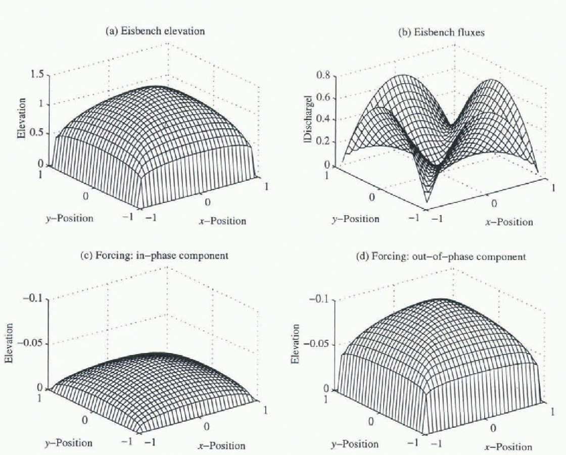
Fig. 1. The EB experiment (Reference Huybrechts and PayneHuybrechts and others, 1996). (a) The Steady-state elevation in sealed units. (b) Absolute dimensionless flux. (c) In-phase component of elevation for 20 ka forcing; note reverse axis. (d) Out-of-phase component of elevation for 20 ka forcing.
Some modes for the perturbation around the Eismint benchmark are shown in Figure 2. Two of these are volumetric modes, while activation of the other two does not result in volume changes but does produce asymmetry in the ice sheets. Corresponding accumulation sampling functions are shown in Figure 3. These show broadly similar patterns, necessarily to the extern that the symmetries between modes and sampling functions are the same, but there are differences in detail between the eigenfunctions and the sampling functions. For example, activation of the slowest mode requires a proportionately greater amount of accumulation nearer the centre; this feature also occurs in 1HD (Reference HindmarshHindmarsh, in press).
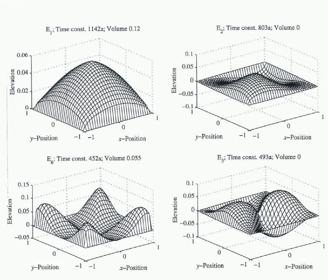
Fig. 2. Eigenfunctions of the EB. Four modes are illustrated; the two lefthand ones are volumetric, while excitation of the two righthand ones results in asymmetry. E number is the mode number. which has standard solution
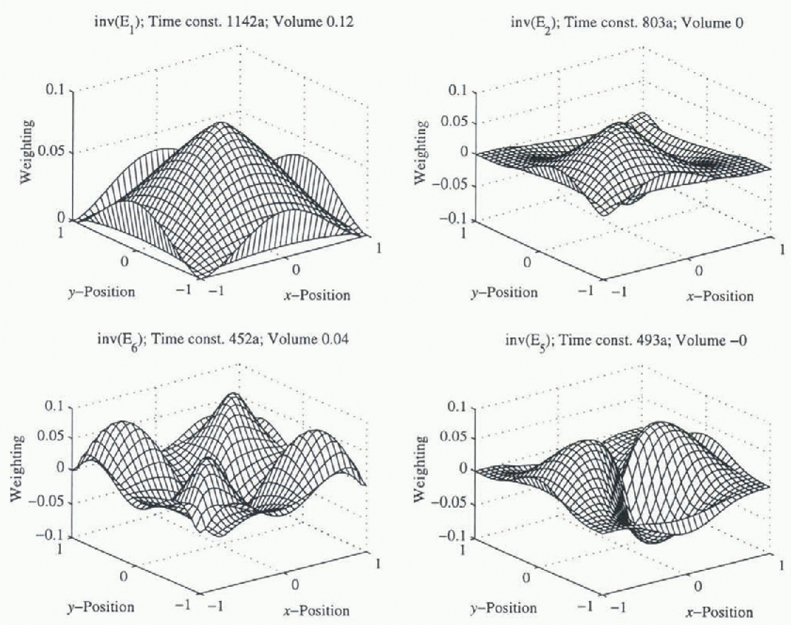
Fig. 3. Accumulation-rate distribution which excites the corresponding made number. This is computed by inverting the eigenfunction matrix.
The sealing relation (e.g. Reference HindmarshHindmarsh, 1990) shows the response of the ice-sheet thickness to changes in the accumulation rate is
. The fact that the accumulation rate is uniform implies that the normalized elevation of the ice-sheet (i.e. normalized by the maximum elevation) is unchanged under uniform changes in accumulation, while the maximum elevation behaves according to this scaling rule. We can linearize the scale rule:

and this is the behaviour that should be followed by the linearized model: a uniform change in accumulation will lead to a uniform relative change in elevation according to this formula.
Calculations with the diseretized operator G show that this behaviour is obtained to round off error for a selection of m and ν. It did not matter whether the zeroth-order solution was computed using finite-difference techniques or was an analytical solution, obtainable for the cases (m,ν) = (0,1), (3,1) (Reference Hindmarsh and PayneHindmarsh and Payne, 1996). This is because it has been ensured that the zeroth-order solution respects continuity “exactly” (i.e. to round off error).
A more complicated case is periodic forcing of the accumulation rate. Consider a system forced at several frequencies k = (1, K)

Here,
or in matrix notation:
where
![]() represents the pointwise Fourier transform of the
accumulation distribution in time. In practice, this formalism is
overcomplicated because there is insufficient data, and the accumulation might
be specified as varying uniformly in space according to a few selected
frequencies.
represents the pointwise Fourier transform of the
accumulation distribution in time. In practice, this formalism is
overcomplicated because there is insufficient data, and the accumulation might
be specified as varying uniformly in space according to a few selected
frequencies.
From the point of view of comparing results, it is more convenient to carry out a spectral analysis of the results of the EB, and compare these with the analytical solution presented above. The elevation at each interior point of the EB grid forms a time series the periodogram of which can be formed (the data are so clean that periodograms suffice). Since the Eismint experiments are forced at one period only, only the amplitude and phase information need to be retrieved at the appropriate frequency. In practice, power might be expected at harmonic frequencies owing to nonlinear effects “beats”), but these will be ignored in the following analysis. The error this introduces is not great.
Thus, for each point of the EB grid, at the fundamental frequency (the
frequency of forcing), the spatial variation of the Fourier components is
considered. More specifically, denote by
![]() � the discrete Fourier transform of the elevation of the
points (xl, yl
) at a frequency w
k (a more intuitive description is provided below). For example,
Figure 1c and d shows the real and
imaginary components of
� the discrete Fourier transform of the elevation of the
points (xl, yl
) at a frequency w
k (a more intuitive description is provided below). For example,
Figure 1c and d shows the real and
imaginary components of
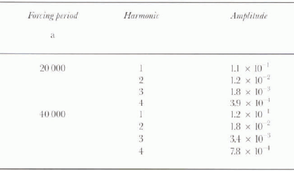
![]() at the forcing period (in this case 20 ka). Table 2 shows the amplitude of the Fourier
transform of the centre-point elevation at selected multiples of the forcing
frequency. The amplitude of the second harmonic is at most 15% of the first
harmonic.
at the forcing period (in this case 20 ka). Table 2 shows the amplitude of the Fourier
transform of the centre-point elevation at selected multiples of the forcing
frequency. The amplitude of the second harmonic is at most 15% of the first
harmonic.
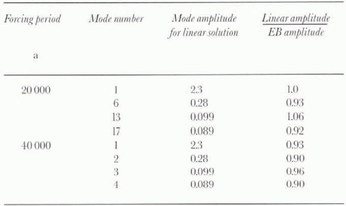
Table 2. The Fourier transformation of the centre elevation in the EB for forcings of 20 and 40 ka. Amplitudes for the first four harmonics are given, showing that non-linear behaviour accounts for between 10 and 14% of the signal
Then, for a given frequency wk the Fourier coefficients can be projected onto the discretized eigenvectors E thus:
where
![]() is the vector formed from
is the vector formed from
![]() and Ck
, formed from Cik
, is a vector of mode coefficients corresponding to the frequency
k Amplitude ∣Ck
∣ and phase information øk
= arg Ck
for each mode i can be computed and compared with
the analytical solution. In practice, this is only applied at the driving
frequency.
and Ck
, formed from Cik
, is a vector of mode coefficients corresponding to the frequency
k Amplitude ∣Ck
∣ and phase information øk
= arg Ck
for each mode i can be computed and compared with
the analytical solution. In practice, this is only applied at the driving
frequency.
It is helpful to consider this visually. The steady-stalte EB profile (Fig. 1a) is subjected to a periodic forcing.
Fhe point elevations are Fourier-transformed to yield the surfaces shown in
Figure 1c and d ; these are the coefficients
![]() . These surfaces can be represented, quite efficiently, as a
series of the eigenfunctions from the linearization and shown in Figure 2. The coefficients
Ck
multiplying the eigenfunctions in this series are obtained by
computing the inner product of the surfaces in Figure 1c and d (the Fourier
coefficients of the forcing of the Eismint experiment) with the sampling
functions shown in Figure 3.
. These surfaces can be represented, quite efficiently, as a
series of the eigenfunctions from the linearization and shown in Figure 2. The coefficients
Ck
multiplying the eigenfunctions in this series are obtained by
computing the inner product of the surfaces in Figure 1c and d (the Fourier
coefficients of the forcing of the Eismint experiment) with the sampling
functions shown in Figure 3.
The accumulation-rate variation specified in the EB is large (a = 0.3 ± 0.2 m a−1) but the maximum error in the perturbation which is associated with oscillation of the first (slowest) mode is 7%. This can be seen from Table 1, which lists the components Cik . (Several have been omitted because symmetry enforces Cik to be zero for uniform accumulation). For forcing at 40 000 years, the error in the computed amplitude for the first few non-zero modes reaches 1% but the dominating contribution comes from the first mode where die error is 6%. Phase lags are around π/2 for both models. For forcing at 20 000 years, where the amplitude deviation is smaller, the accuracy is higher. On to these errors should be added the errors arising from ignoring the higher harmonics, making the total error about 20%.
These errors are not negligible but the EB is a fairly severe test with accumulation amplitude two-thirds of the mean accumulation, somewhat larger than those experienced during the Ice Age by either the Aniarctic or the Greenland ice sheets. The smaller perturbation associated with the shorter period forcing has a smaller error.
Normal-Mode Analysis of Some Antarctic DEMs
Two Antarctic digital elevation models (DKM), both with 80 km grids (Reference Budd and SmithBudd and Smith, 1982, Reference Budd and Smith1985; Reference Bamber and HuybrechtsBamber and Huybrechts, 1996) with associated grids of basal elevation and surface accumulation rate were used. Balance fluxcs were calculated and the normal modes computed. These coarse grids were used because it is still a formidable computational task to compute all the modes for finer grids, and it seemed desirable to compute all the modes in smaller test cases rather than truncating arbitrarily with finer grids. The Reference Bamber and HuybrechtsBamber and Huybrechts (1996) elevation grid is more accurate than the Reference Budd and WarnerBudd and Smith (1985) grid, but there is an issue of the sensitivity of the slower modes to date uncertainty. In both computations the accumulation data from Reference Budd and WarnerBudd and Smith (1985) are used. Reference HindmarshHindmarsh (in press) has discussed the robustness of one-dimensional (1-D) perturbations to the ice-sheet equation. In this case, a Sturm-Liou-ville equation is obtained and the robustness of their spectra to model (not solution) perturbation is well understood (Reference PrycePryce, 1993). While Sturm-Liouville forms cannot be obtained in higher dimensions, the robustness property is expected to be maintained.
Balance fluxes and normal modes were computed in the manner described above using ν = 3, m = 5, corresponding to internal deformation according to a Reference GlenGlen (1955) rheology. A puzzling feature was the presence of eigenvalues and vectors with non-zero imaginary parts. The non-zero parts of the eigenvalues were at most no more than a few per cent of the corresponding real parts. There are several possible causes for this but, if one considers the ice-sheet equation in the 1-D form
and expands:

then, if
which is a first-order hyperbolic equation. In such a case, one is less surprised to see complex eigenvalues and they may therefore arise from rugose basal topography. The argumenl of the eigenvalues (i.e. Im(λ)/Re(λ)) is plotted in Figure 4. Complex eigenvectors only occur when complex eigenvalues exist. Figure 4 shows that this problem only exists for higher-mode numbers. The following discussion refers to the real parts of the modes.
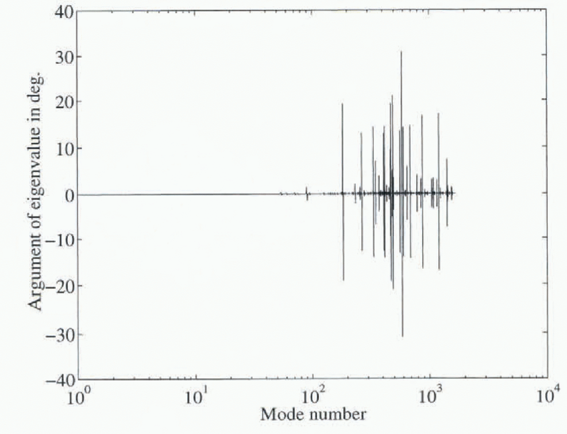
Fig. 4. The argument of the eigenvalue plotted against mode number. Non-zero arguments are a numerical artefact. They do not appear in modes of < order 100.
The six slowest modes for each case are shown in Figures 5 and 6, together with associated time constants and volumes relative to the slowest mode. The results are broadly similar and the percentage differences between the computed time constants are smaller than the uncertainty in the rheological indices ν and m.
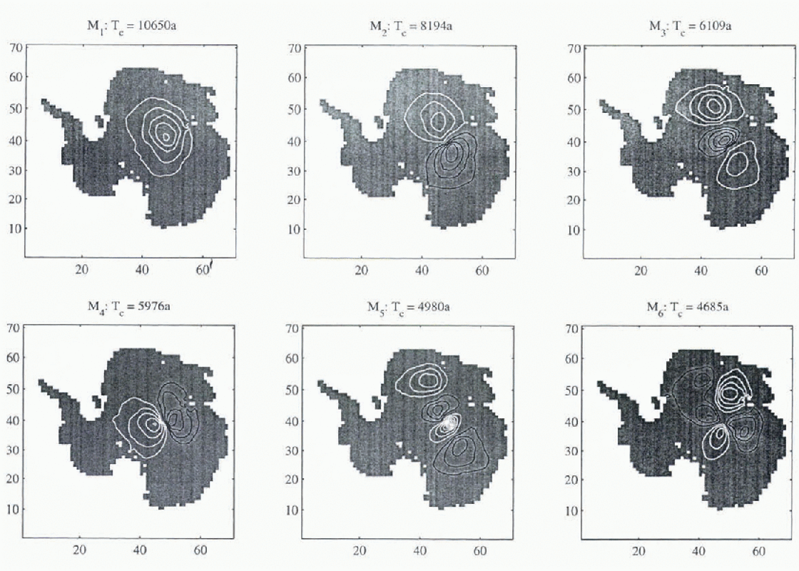
Fig. 5. Six slowest modes computed from the MSSL dataset (Reference Bamber and HuybrechtsBamber and Huybrechts, 1996). Associated time constants and relative volumes are indicated. Contour interval 0.2; black and white contours are of Opposite sign.
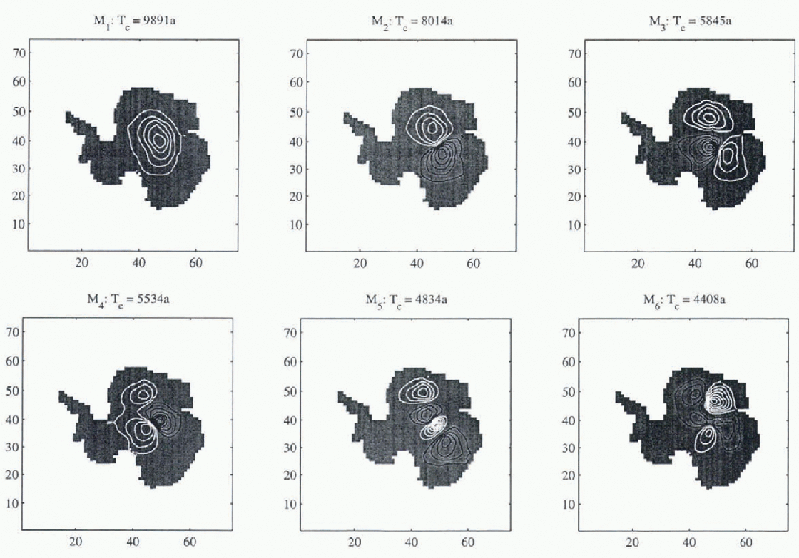
Fig. 6. Six slowest modes computed from the UM dateset (Reference Budd, Jacka, Jenssen, Radok and YoungBudd and others, 1982). Associated time constants and relative volumes are indicated. Contour interval 0.2; black and while contours are of opposite sign.
A significant result is that these low-order modes are smooth, despite the use of accurate date in the MSSL data-set. Thus, the process of computing the normal modes in effect filters the data in the sense that small-scale spatial variation is only excited by small-scale forcing.
These modes are clearly East Antarctic modes and relate to the fact that the time constants for Wast Antarctica are greater than for West Aniarctica owing to the low accumulation rates (e.g. Reference HindmarshHindmarsh, 1990). Evidently, the Lambert Basin splits the glaciodynamic response of East Antarctica asunder. The temptation should be resisted to conclude that coarse grids are sufficient to compute the no mal modes of an ice sheet. The analysis of Reference Budd and WarnerBudd and Warner (1996) shows how flow is directed into streams and it can be seen from the perturbation Equation (11) that spatial variations in the zeroth-order discharge might well have a significant effect.
The accumulation-rate sampling distributions (i. e. the rows of E−1) are shown in Figure 7. Their spatial structure is broadly similar to the modes, as is the case in 1HD (Reference HindmarshHindmarsh, in press), but owing to their non-orthogonality, do not excite only the corresponding mode, as compared to the orthogonal functions th at appear in 1HD.
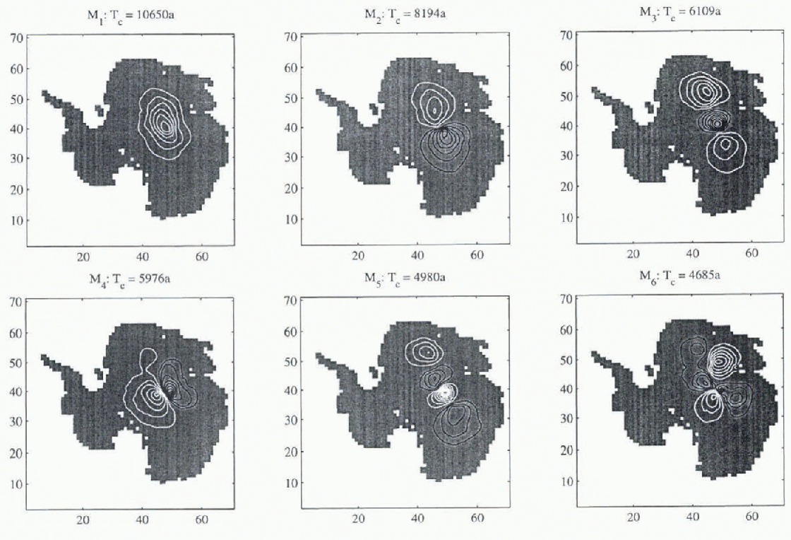
Fig. 7. Distribution of accumulation that optimally excites the corresponding mode, MSSL dataset. These accumulation distributions will excite other modes as they are not orthogonal. Contour interval 0.2; black and white contours are of apposite sign.
Volumetric spectra (i.e. the eigenfunction volume plotted against its associated time constants) are shown in Figure 8. The slowest modes have time-steps of around 10 000 years, which can be predicted from the scale relationship H/a (2n + 2). The volumetric spectrum indicates the relaxation time-scales of volumetric significance. The modes with short time constants do, in sum of absolute magnitude, represent a considerable volume but these modes are associated with spatial length scales smaller than likely variation in the accumulation rate and will not therefore be activated significantly. Thus, most of the volumetric response
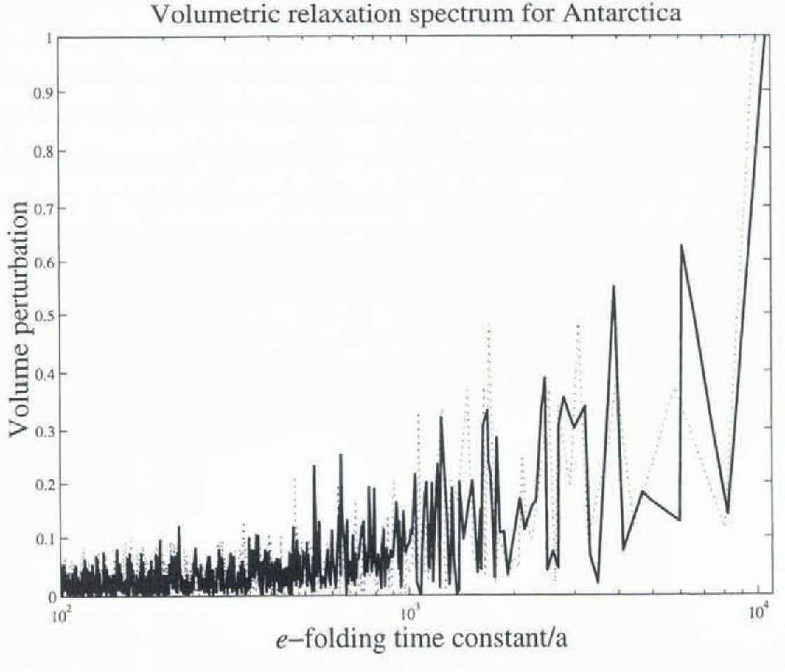
Fig. 8. Volumetric spectrum: made volume plotted against the associated time constant. MSSL data plotted in heavy line, UM dataset in dotted line.
Table 3. The amplitudes of some spatial modes in the EB configuration for forcings of period 20 and 40 ka, compared with the linear solutions. The linear amplitudes depend on the forcing period but tht effect is too small to be seen at the quoted accuracy seems to be concentrated between 1000 and 10 000 years. This is consistent with conclusions obtained by Reference HuybrechtsHuybrechts (1992) using a non-linear thermomcchanically coupled model.
It is possible, using the procedure described in Equations (18) to (20), to compute the response of the ice sheet to changes in the accumulation rate. The eigenfunctions can be used to decompose the spatial distribution of the accumulation and lhe evolution split between fast, slaved modes (with high wave-number spatial variability) the instantaneous contribution of which is described by Equation 18a and the slow, large spatial-scale modes the evolution of which is described by the dynamical Equation (19). In this way, the spatial structure associated with the fast modes can be retained in the evolution calculation. In non-linear models, date inconsistencies associated with the fast modes lend to cause numerical problems (e.g. Reference Oerlemans and van der VeenOerlemans and Van der Veen, 1984) and data inconsistencies are relaxed out by running the model. Space limitations preclude further discussion of this important application.way, the spatial structure associated with the fast modes can be retained in the evolution calculation. In non-linear models, date inconsistencies associated with the fast modes lend to cause numerical problems (e.g. Reference Oerlemans and van der VeenOerlemans and Van der Veen, 1984) and data inconsistencies are relaxed out by running the model. Space limitations preclude further discussion of this important application.way, the spatial structure associated with the fast modes can be retained in the evolution calculation. In non-linear models, date inconsistencies associated with the fast modes lend to cause numerical problems (e.g. Reference Oerlemans and van der VeenOerlemans and Van der Veen, 1984) and data inconsistencies are relaxed out by running the model. Space limitations preclude further discussion of this important application.way, the spatial structure associated with the fast modes can be retained in the evolution calculation. In non-linear models, date inconsistencies associated with the fast modes lend to cause numerical problems (e.g. Reference Oerlemans and van der VeenOerlemans and Van der Veen, 1984) and data inconsistencies are relaxed out by running the model. Space limitations preclude further discussion of this important application.
Conclusions
Of the three options discussed for initialization, the easiest one, which uses observed elevations in the zeroth-order solution, seems to be a feasible way of initializing models. This is because the smaller-scale structure in the zeroth-order solutions is not manifested in the low-order modes of the perturbed solution. The practical consequence of this is high accuracy. Normal-mode analyses permit small spatial structure to be retained in models without being relaxed out. where it is due to data inconsistency or causing numerical instability. There remains a problem of how to deal with sink holes.
The normal modes of two Antarctic DEMs have been computed. The differences in elevation cause relatively small variations in the spectrum and the qualitative features of the eigenfunctions remain similar for slower modes. The t-folding relaxation time constant for East Antarctica is around 10 000 years. The volumetric aspect of the relaxation of Antarctica has been computed, with the most significant response occurring on time-scales between 1000 and 10 000 years. What causes the spatial structure of the modes is not obvious and requires further investigation. Better physics, in particular the representation of grounding-line motion and of sliding, should be available in the future.
Acknowledgements
I had instructive conversations with J. Bamber, W. Budd, C. Raymond, D. Sorensen, R. Warner and E. Waddington. J. Bamber and R. Warner provided me with date sets for Antarctica. G. K. C. Clarke's review made me rethink the structure of the paper.


